1. Introduction
Spherical robots with unique structures have gradually become the focus of research on new special robots, and are widely used in a variety of environments [Reference Bujňák, Pirník, Rástočny`, Janota, Nemec, Kuchár, Tichy` and Łukasik1–Reference Bahar, Abdullah, Aras, Harun and Zohedi3]. After years of development, the spherical robot structure has been innovated and improved in a variety of ways [Reference Chase and Pandya4–Reference Diouf, Belzile, Saad and St-Onge6]. There are many spherical robot structures, and one of the main development lines is the pendulum spherical robot. The core structure of the pendulum spherical robot is an internal pendulum and an external spherical shell. The center of gravity of the robot is controlled by changing the angle of the pendulum [Reference Ahn and Lee7–Reference Asiri, Khademianzadeh, Monadjemi and Moallem10].
At present, many studies on spherical robot motion mainly focus on horizontal plane motion. In order to accurately describe the motion of spherical robots, many scholars have established motion models of spherical robots. On the basis of motion analysis, Sun et al. [Reference Sun, Wang, Jia and Liu11] established a complete dynamic model of the BYQ-3 spherical robot based on the Kane equation modeling method of vector operation. Zheng et al. [Reference ZHENG, ZHAN, LIU and CAI12] constructed a simple spherical robot motion model according to the characteristics of spherical motion. Kayacan [Reference Kayacan, Bayraktaroglu and Saeys13] studied a decoupled motion model of a pendulum spherical robot. Li et al. [Reference Li, Wang and Ji14] used Maggi’s equations without the Lagrange’s multipliers to construct a spherical robot model. Azizi [Reference Azizi and Naderi15] used Euler’s parameter method and Cairn’s method to derive the kinematic and dynamic equations of the whole system. Based on the Newton-Euler formula, Ghariblu [Reference Ghariblu16] solved the robot’s dynamical equations. Kilin et al. [Reference Kilin, Pivovarova and Ivanova17] used the Lagrangian method to model and find the fixed point of the spherical robot.
Based on these spherical robot models, scholars have designed a variety of spherical robot motion control systems. PID controllers are widely used in robot control [Reference Diouf, Belzile, Saad and St-Onge6]. Zhang et al. [Reference Zhang, Jia, Sun and Gong18] used a PI controller to achieve real-time control of the entire system. Then, the genetic algorithm was applied to the setting and optimization of PI parameters to improve the stability of the system. Zhao [Reference Zhao, Wang, Sun and Li19] used a PID controller to control a double-pendulum spherical robot. Matin [Reference Matin, Piltan, Cheraghi, Sobhani and Rahmani20] designed The minimum rule base PID Fuzzy Sliding Mode Controller for spherical robots and simulated validation. Sadeghian [Reference Sadeghian and Masouleh21] designed PD and PID controllers for spherical robots using a pole-based configuration method. However, in complex nonlinear systems, the performance of PID controllers is still insufficient. Gradually, nonlinear controllers are being applied to spherical robots. Among them, several mainstream control systems are divided into sliding mode control and its improvement, adaptive control and its improvement, active disturbance rejection and other anti-disturbance controllers, intelligent control methods, etc. In sliding mode control, Kayacan [Reference Kayacan, Kayacan, Ramon and Saeys22] proposed a control method combining an adaptive neural fuzzy controller with a sliding mode control theory. Yue [Reference Yue, Liu, Wei and Hu23] improved the sliding mode algorithm to improve the adaptive ability of the controller. Roozegar [Reference Roozegar, Ayati and Mahjoob24] used terminal sliding mode control to estimate the disturbance of spherical robots. Taheri [Reference Andani, Ramezani, Moazami, Cao, Arefi and Zargarzadeh25] proposed a system combining a neural network observer and an improved sliding mode for tracking control of spherical robots. Ma [Reference Ma, Sun and Song26] proposed a new hierarchical sliding mode control, which is more suitable for the drive structure of spherical robots. Zhou [Reference Zhou, Xu and Wu27] proposed a method combining fractional order calculus and layered sliding mode under the condition of input saturation. Salemizadeh [Reference Parizi, Salemizadehparizi, Vanaei, Karimi and Komijani28] proposed a novel hybrid super-twisting fractional-order terminal sliding mode controller method for external disturbance and noise, which can achieve disturbance cancelation and improve response speed. Liu [Reference Liu, Wang, Guan, Hu, Zhang, Jin, Wang, Hao and Li29] proposed a hierarchical terminal sliding mode controller and used it in hardware systems. In adaptive control, many adaptive control methods rely on sliding mode control methods [Reference Kayacan, Kayacan, Ramon and Saeys22, Reference Yue, Liu, Wei and Hu23, Reference Ma, Sun and Song26]. Roozegar [Reference Roozegar, Mahjoob and Ayati30, Reference Roozegar, Mahjoob and Ayati31] also applied model-referenced adaptive control to spherical robot control. With the development of intelligent technology, intelligent control has also been gradually applied to spherical robots. Liu [Reference Liu, Wang, Guan, Wang, Jin, Hu, Ren, Hao, Zhang and Li32] combined adaptive RBF neural network with sliding mode control for motion control of spherical robots. Ren [Reference Ren, Wang, Liu, Jin, Wang, Liu, Zhang, Hu and Li33] designed a model predictive control-based instruction planning controller. Cai [Reference Cai, Zhan and Xi34] used a single input, multiple output PID controller, and a neural network controller to compensate for the nonlinearity of the actuator.
Research on the control of spherical robots in planar motion has gradually deepened. However, as a type of special robot, spherical robots possess diverse application environments. Sloped environments, such as mountainous areas, urban settings, and grasslands, are common in various applications. These inclined terrains significantly impact the motion of spherical robots. Hogan conducted a dynamic simulation of a spherical robot’s motion in Martian craters [Reference Hogan and Forbes35]. Roozegar investigated the motion of spherical robots on inclined surfaces and employed a fuzzy PID controller and a switching system to control the robot’s movement [Reference Roozegar and Mahjoob36]. Subsequently, he used a terminal sliding mode controller to study the motion control of spherical robots on variable-slope surfaces[Reference Roozegar, Ayati and Mahjoob24]. Moazami et al. investigated the motion of spherical robots on three-dimensional curved surfaces by analyzing their structural design [Reference Moazami, Palanki and Zargarzadeh37]. Sabet et al. proposed a dynamic model combined with energy analysis to achieve motion planning for spherical robots on uneven terrains [Reference Sabet, Poursina, Nikravesh, Reverdy and Agha-Mohammadi38]. Compared to planar environments, motion control of spherical robots on slopes has been less explored, with existing studies focusing primarily on obstacle traversal and curved-surface trajectory analysis. Roozegar and Zhan [Reference Zhan, Cai and Yan39] examined the locomotion of spherical robots on inclined surfaces. While Zhan’s study emphasized a wheeled spherical robot with limited slope-specific analysis, Roozegar concentrated on the climbing motion of pendulum-driven spherical robots. However, their analyses and descriptions of equilibrium states on inclined surfaces remain overly generalized.
Meanwhile, conventional PID control and its variants have shown limited effectiveness in governing spherical robots within complex environments, while the design and implementation of novel intelligent methods remain challenging. To address this, backstepping control constructs control laws based on the dynamic model of the system, achieving stability through mathematical manipulation of control variables, with its elegant mathematical formulation demonstrating significant advantages. In early research, the backstepping method was applied to design control laws for nonholonomic mobile robots [Reference Fierro and Lewis40]. This design concept was also utilized to enhance trajectory tracking performance in vehicles [Reference David and III41]. Furthermore, the backstepping method has been extended to formation control problems [Reference Dierks and Jagannathan42]. Cai et al. proposed a backstepping-based control strategy specifically for path tracking [Reference Cai, Zhan and Xi43]. Bai et al. applied backstepping control to spherical robots for trajectory tracking tasks, including straight-line and circular motion [Reference Bai, Svinin and Yamamoto44]. Hoang proposed a backstepping-based method focused on the rolling motion control of two-wheeled spherical robots [Reference Dong, Lee, Woo and Leb45]. Currently, the backstepping method is predominantly utilized for trajectory tracking in mobile robots, with limited application to angle control in pendulum-driven spherical robots.
According to the above review, research on the motion of spherical robots on inclined surfaces remains limited. In particular, studies focusing on the equilibrium states of spherical robots on slopes are even scarcer, and existing equilibrium formulations face significant challenges in practical applications. Although various advanced control theories have been applied to slope control methods, it remains unclear whether a simple and feasible control approach can achieve effective control for spherical robots, necessitating further investigation.
The main contributions of this paper are divided into two parts:
Accurate Equilibrium Modeling for Spherical Robots on Slopes: Addressing the issue of insufficient precision in describing the actual center of gravity in existing equilibrium equations for spherical robots, this paper analyzes the equilibrium states of spherical robots on inclined surfaces. Using the virtual displacement method, the pendulum angle is correlated with parameters such as the mass ratio of the spherical shell to the pendulum, the radius ratio of the spherical shell to the pendulum, and the slope angle. Based on this, the equilibrium equation for spherical robots on inclined surfaces is derived.
Control Strategy for Spherical Robots on Slopes: To address the control challenges of spherical robots on slopes, this study simplifies undulating terrains into ideal slopes with varying gradients. Building on this, the climbing control of spherical robots is categorized and investigated under two scenarios: known slope angles and unknown slope angles. A backstepping controller is designed for spherical robots moving on inclined surfaces. For unknown slope angles, a parameter adaptation method is employed to estimate the slope parameters, and the performance of the backstepping controller is adjusted accordingly to achieve stable system control.
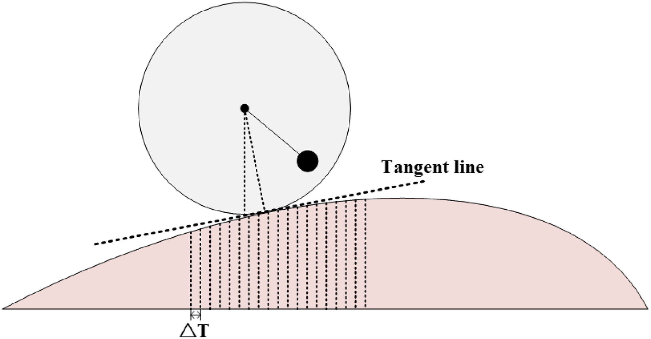
Schematic diagram of the movement of a spherical robot on a rough road.

2. Spherical robot modeling
In different environments, slopes can vary significantly in form, such as steep slopes and gentle slopes (Figure 1). These slopes can be represented as different curves on a two-dimensional plane. Since the spherical robot contacts the slope at a single point, the motion of the spherical robot on the slope can be simplified. By constructing a tangent line at the contact point, this tangent can be treated as an ideal inclined plane, where the slope of the tangent represents the climbing gradient. The motion of the spherical robot is sampled at intervals of
 $\Delta T$
, and the slope is updated accordingly at each interval
 $\Delta T$
.
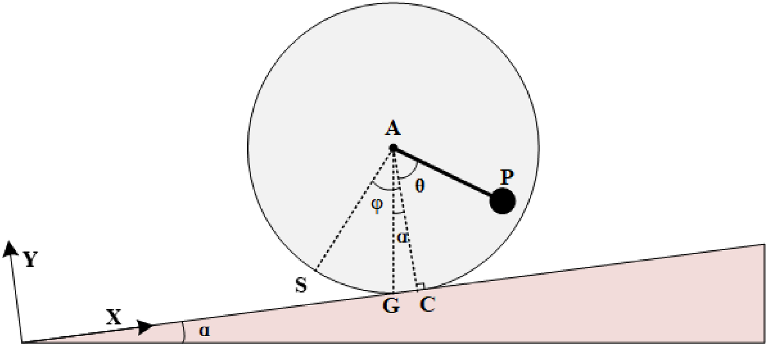
The motion of the spherical robot on an ideal inclined surface is illustrated in Figure 2. The theoretical study in this paper is divided into two main parts. Equilibrium Analysis: The first part focuses on analyzing the stable states of the spherical robot on inclined surfaces, establishing the relationship between the pendulum angle and the slope gradient. Dynamic Modeling: The second part involves analyzing the dynamic model of the spherical robot moving on slopes, which serves as the foundation for subsequent control algorithm design.
2.1. Equilibrium analysis
On such slopes, the spherical robot is treated as a conservative force system, and the static analysis is performed according to the imaginary displacement principle. Taking the contact point of the spherical shell as the zero potential energy reference surface, the positions of point A and point P can be represented as follows in Figure 2.
Schematic diagram of the inclined plane motion of a spherical robot.

A point:
 \begin{equation} y_1=r \cdot \cos \alpha \end{equation}
P point:
 \begin{equation} y_2=r \cos \alpha -l \cos (\alpha +\theta ) \end{equation}
It can be seen that under equilibrium conditions, the position of the system can be completely determined by the parameter
 $\alpha$
, and it can be regarded as a single-degree-of-freedom system in the process of ramp stabilization. Give the system a set of imaginary displacements
 $\delta y_1$
,
 $\delta y_2$
, and
 $\delta \alpha$
, and the relationship between them is given by the variation of the previous two equations.
 \begin{equation} \delta y_1=-r \sin \alpha \delta \alpha \end{equation}
 \begin{equation} \delta y_2=(\!-r \sin \alpha +l \sin (\alpha +\theta )) \delta \alpha \end{equation}
The sum of the virtual works of the active force in equilibrium is satisfied:
 \begin{equation} \sum \delta W=m_A g \delta y_1+m_P g \delta y_2=0 \end{equation}
 \begin{equation} \sum \delta W=\left [-m_A g r \sin \alpha +m_P g(-r \sin \alpha +l \sin (\alpha +\theta ))\right ] \delta \alpha =0 \end{equation}
 \begin{equation} -\left (m_A g+m_P g\right ) r \sin \alpha +m_P g l \sin (\alpha +\theta )=0 \end{equation}
To derive theta:
 \begin{equation} \theta =\sin ^{-1}\left [\left (\frac {m_A}{m_P}+1\right ) \frac {r}{l} \sin \alpha \right ]-\alpha \end{equation}
Compared to the article by researchers at Roozegar [Reference Roozegar, Ayati and Mahjoob24], the balance equation for the spherical robot proposed by Roozegar primarily includes variables such as the center of mass and radius. The center of mass has significant errors in actual calculations. The balance equation derived in this paper Eq. (8) is approximately similar to the aforementioned equation, but it substitutes the center of mass variable with the ratio of the spherical shell mass to the pendulum mass. By incorporating the radius of the spherical shell and the pendulum length, a more concise expression for the balance equation of the pendulum-based spherical robot is obtained.
2.2. Dynamic modeling
In the process of climbing,
 $\varphi$
is the rolling Angle of the shell and
 $\theta$
is the rotation Angle of the pendulum. Assuming that the slope
 $\alpha$
and the pendulum swing Angle
 $\theta$
are known, the gyroscope measures
 $\alpha +\theta$
, and the balance control is carried out.
According to the motion of spherical robot, the Lagrange dynamic model is constructed, and the coordinate system
 $O-XYZ$
is established with the slope surface as the
 $X$
-axis. The spherical robot is assumed to roll without sliding. The mass of the shell is evenly distributed.
In the spherical shell coordinate system, the angular velocity of the spherical shell can be expressed as:
 \begin{equation} \boldsymbol{\omega _s^{\mathbf{0}}}=(0,0,-\dot {\varphi })^T \end{equation}
Using the base coordinate system
 $O-XYZ$
as reference, the angular velocity of the spherical shell is
 $\boldsymbol{\omega _s}=\boldsymbol{R_1} \boldsymbol{\omega _s^0}$
, where the rotation matrix
 $\boldsymbol{R}_{\mathbf{1}}=\left [\begin{array}{c@{\quad}c@{\quad}c} \cos \varphi & \sin \varphi & 0 \\[4pt] -\sin \varphi & \cos \varphi & 0 \\ 0 & 0 & 1 \end{array}\right ]$
.
The spherical robot rolls with the ground without slip. It can be seen that
 $\boldsymbol{v_c}$
is:
 \begin{equation} \boldsymbol{v_c}=\boldsymbol{v_s}+\boldsymbol{\omega _s} \times \boldsymbol{r} \end{equation}
where
 $\boldsymbol{v_s}$
is the velocity of the shell. Shell radius
 $\boldsymbol{r}=\left (0,-\mathrm{r}_0, 0\right )^T$
. The velocity
 $\boldsymbol{v_c}=\left (0,0, 0\right )^T$
is obtained from the non-slip rolling. We can get
 $\boldsymbol{v_s}$
as:
 \begin{equation} \boldsymbol{v_s}=-\boldsymbol{\omega _s} \times \boldsymbol{r} \end{equation}
For the pendulum of a spherical robot, in the pendulum coordinate system, the angular velocity of the pendulum can be expressed as
 \begin{equation} \boldsymbol{\omega }_{\boldsymbol{p}}^{\mathbf{0}}=(0,0, \dot {\theta })^T \end{equation}
Taking the base coordinate system
 $O-XYZ$
as a reference, the angular velocity of the pendulum is
 $\boldsymbol{\omega _p}=\boldsymbol{R_2} \boldsymbol{\omega _p^0}$
. where the rotation matrix is
 $\boldsymbol{R}_{\mathbf{2}}=\left [\begin{array}{ccc}\cos \theta & -\sin \theta & 0 \\ \sin \theta & \cos \theta & 0 \\ 0 & 0 & 1\end{array}\right ]$
.
The linear velocity of the pendulum is
 \begin{equation} \boldsymbol{v_p}=\boldsymbol{v_s}+\boldsymbol{\omega _p} \times \boldsymbol{l} \end{equation}
Wherein, the pendulum length is:
 $\boldsymbol{l}=\left (0,-l_0, 0\right )^T$
Select the generalized coordinates as
 $\boldsymbol{q}=[\varphi, \theta ]^T$
,
 $\boldsymbol{Q}=[0, \tau ]^T$
. The Lagrangian method was used to construct the dynamic model of the spherical robot.
 \begin{equation} \frac {d}{d t}\left (\frac {\partial L}{\partial \dot {\boldsymbol{q}}}\right )-\frac {\partial L}{\partial \boldsymbol{q}}=\boldsymbol{Q} \end{equation}
where
 $L=T-V$
. The kinetic energy of the spherical shell and the pendulum is composed of two parts
 $T_s=\frac {1}{2} m_s \boldsymbol{v}_s^2+\frac {1}{2} I_s \boldsymbol{\omega }_s^2$
,
 $T_p=\frac {1}{2} m_p \boldsymbol{v}_p^2+\frac {1}{2} I_p \boldsymbol{\omega }_p^2$
. In the process of climbing, considering the influence of slope, the potential energy of the spherical robot is
 $V_s=m_s g\left (x \sin \alpha +r_0 \cos \alpha \right )$
,
 $V_p=m_p g\left (x \sin \alpha + r_0 \cos \alpha -l_0 \cos (\alpha +\theta )\right )$
 \begin{equation} M(\boldsymbol{q}) \ddot {\boldsymbol{q}}+V(\boldsymbol{q}, \dot {\boldsymbol{q}})=\boldsymbol{Q} \end{equation}
where
 $\boldsymbol{M}(\boldsymbol{q})=\left [\begin{array}{c@{\quad}c}I_s+m_p \mathrm{r}_0^2+m_s \mathrm{r}_0^2 & l_0 m_p \mathrm{r}_0 \\[4pt] l_0 m_p \mathrm{r}_0 & m_p l_0^2+I_p\end{array}\right ]$
,
 $ \boldsymbol{V}(\boldsymbol{q}, \dot {\boldsymbol{q}})=\left [\begin{array}{c}0 \\ g l_0 m_p \sin (\alpha +\theta )\end{array}\right ]$
3. Controller design
Considering the complexity of the slope motion of the spherical robot, this paper simplifies the motion situation and divides it into two parts: the motion control of the spherical robot on the slope and the adaptive design of the slope parameters in the controller. Considering the whole system, the state-space equations for the angle
 $\theta$
of the pendulum and the angle
 $\varphi$
of the spherical shell are constructed according to Eq. (15).
where
 $\boldsymbol{x}=[\theta, \dot {\theta }, \varphi, \dot {\varphi }]^T$
,
 $ x_1=\theta$
,
 $ x_2=\dot {\theta }$
,
 $ x_3=\varphi$
,
 $ x_4=\dot {\varphi }$
.
 \begin{equation} \left \{\begin{array}{l} \dot {x}_1=x_2 \\[10pt] \dot {x}_2=\displaystyle\frac {\left (u-g l_0 m_p \sin (\alpha +\theta )\right ) \cdot \left (I_s+m_p r_0{ }^2+m_s r_0{ }^2\right )}{I_p I_s+I_s l_0{ }^2 m_p+I_p m_p r_0{ }^2+I_p m_s r_0{ }^2+l_0{ }^2 m_p m_s r_0{ }^2} \\[14pt] \dot {x}_3=x_4 \\[8pt] \dot {x}_4=\displaystyle\frac {-l_0 m_p r_0\left (u-g l_0 m_p \sin (\alpha +\theta )\right )}{I_p I_s+I_s l_0{ }^2 m_p+I_p m_p r_0{ }^2+I_p m_s r_0{ }^2+l_0{ }^2 m_p m_s r_0{ }^2} \end{array}\right . \end{equation}
In the simulation experiments, it is found that the slope has a great influence on the pendulum angle of the spherical robot. However, the slope has a negligible effect on the spherical shell angle. At the same time, since the motor torque directly controls the spherical robot pendulum, the backstepping controller for climbing is only designed for the angle
 $\theta$
. The equation of state with respect to theta is constructed. where
 $\boldsymbol{x}=[\theta, \dot {\theta }]^T$
,
 $ x_1=\theta$
,
 $ x_2=\dot {\theta }$
.
 \begin{equation} \left \{\begin{array}{c} \dot {x}_1=x_2 \\[12pt] \dot {x}_2=\displaystyle\frac {\left (u-g l_0 m_p \sin \left (\alpha +x_1\right )\right ) \cdot \left (I_s+m_p r_0{ }^2+m_s r_0{ }^2\right )}{I_p I_s+I_s l_0{ }^2 m_p+I_p m_p r_0{ }^2+I_p m_s r_0{ }^2+l_0{ }^2 m_p m_s r_0{ }^2} \end{array}\right . \end{equation}
Construct the Lyapunov function
 $V_1$
.
 \begin{equation} V_1=\frac {1}{2} e_1{ }^2 \end{equation}
 \begin{equation} \dot {V}_1=e_1 \dot {e}_1=e_1\left (\dot {x}_{1 d}-x_2\right ) \end{equation}
If an ideal state value exists for
 $x_2$
, denoted as
 $x_{2 d}$
, we define
 $x_{2 d}$
to satisfy the equation:
 $x_{2 d}=\dot {x}_{1 d}+k_1 e_1$
, where
 $k_1$
is a tuning parameter. Consequently, the time derivative of the Lyapunov function
 $V_1$
becomes
 $\dot {V}_1=-k_1 e_1{ }^2$
,which is negative definite (
 $\dot {V}_1\leq 0$
), ensuring system stability.
In real-world systems, the state variable
 $x_2$
deviates from its ideal value
 $x_2$
. Thus, we define the tracking error for
 $x_2$
as
 $e_2=x_{2 d}-x_2$
. By differentiating, we obtain:
 \begin{equation} \dot {e}_2=\dot {x}_{2 d}-\dot {x}_2=\ddot {x}_{1 d}+k_1 \dot {e}_1-\frac {\left (u-g l_0 m_p \sin (\alpha +\theta )\right ) \cdot \left (I_s+m_p r_0{ }^2+m_s r_0{ }^2\right )}{I_p I_s+I_s l_0{ }^2 m_p+I_p m_p r_0{ }^2+I_p m_s r_0{ }^2+l_0{ }^2 m_p m_s r_0{ }^2} \end{equation}
Substituting the error
 $e_2=x_{2 d}-x_2$
and the ideal state definition
 $x_{2 d}=\dot {x}_{1 d}+k_1 e_1$
into Eq. (19), the time derivative of the Lyapunov function
 $\dot {V_1}$
can be rewritten as:
 \begin{equation} \dot {V}_1 = -k_1 e_1^2 + e_1 e_2 \end{equation}
Through Eq. (21), the error
 $e_2$
is linked to the Lyapunov function derivative
 $\dot {V}_1$
.
During the motion of the spherical robot, the knowledge of the slope angle
 $\alpha$
(whether it is known or unknown) affects the accuracy of the controller parameters. This paper discusses two scenarios based on this condition.
Case 1: The slope angle
 $\alpha$
is treated as a known parameter. Physically, this represents a slope with a constant gradient. As mentioned earlier, the error
 $e_2$
exists. To achieve system stability, the Lyapunov function
 $V_2$
is constructed as follows:
 \begin{equation} V_2 = V_1 + \frac {1}{2} e_2^2 \end{equation}
Then, by taking the derivative of
 $V_2$
, we obtain:
 \begin{equation} \dot {V}_2 = \dot {V}_1 + e_2 \dot {e}_2 \end{equation}
Furthermore, substituting Eq. (20) into Eq. (23) yields:
 \begin{equation} \dot {V}_2 = \dot {V}_1 + e_2 \left ( \ddot {x}_{1d} + k_1 \dot {e}_1 - \frac {(u - gl_0 m_p \sin (\alpha + \theta )) \cdot (I_s + m_p r_0^2 + m_s r_0^2)}{I_p I_s + I_s l_0^2 m_p + I_p m_p r_0^2 + I_p m_s r_0^2 + l_0^2 m_p m_s r_0^2} \right ) \end{equation}
To ensure that
 $\dot {V}_2$
is negative definite, and combining with Eq. (21), the control law
 $u$
is designed as:
 \begin{equation} u = \frac {(\ddot {x}_{1d} + k_1 \dot {e}_1 + k_2 e_2 + e_1) \cdot (I_p I_s + I_s l_0^2 m_p + I_p m_p r_0^2 + I_p m_s r_0^2 + l_0^2 m_p m_s r_0^2)}{I_s + m_p r_0^2 + m_s r_0^2} + gl_0 m_p \sin (\alpha + x_1) \end{equation}
where
 $k_2$
is a tuning parameter.
At this point,
 $\dot {V}_2$
can be expressed as:
 \begin{equation} \dot {V}_2 = -k_1 e_1^2 - k_2 e_2^2 \end{equation}
When the slope is known, the system is stable if the control input satisfies Eq. (25), where
 $V_2 \geq 0, \dot {V}_2 \leq 0$
.
Case 2: The slope angle
 $\alpha$
is unknown, meaning
 $\alpha$
is treated as an unknown parameter. Internally, the spherical robot lacks an effective means to measure the slope. To address this, this paper introduces an estimated value
 $\hat {\alpha }$
, where
 $\hat {\alpha }$
is the estimated value of
 $\alpha$
. Furthermore, the estimation error
 $\tilde {\alpha }$
is defined as
 $\tilde {\alpha }=\hat {\alpha }-\alpha$
. Typically, the actual ideal slope angle
 $\alpha$
can be considered constant, i.e.,
 $\dot {\alpha }=0$
. Therefore,
 $\dot {\tilde {\alpha }}=\dot {\hat {\alpha }}$
:
When the slope angle is unknown, the slope in the control law is replaced by its estimated value
 $\hat {\alpha }$
, and Eq. (25) is updated as follows:
 \begin{equation} u = \frac {(\ddot {x}_{1d} + k_1 \dot {e}_1 + k_2 e_2 + e_1) \cdot (I_p I_s + I_s l_0^2 m_p + I_p m_p r_0^2 + I_p m_s r_0^2 + l_0^2 m_p m_s r_0^2)}{I_s + m_p r_0^2 + m_s r_0^2} + gl_0 m_p \sin (\hat {\alpha } + x_1) \end{equation}
Taking into account the slope estimation error, the Lyapunov function
 $V_3$
is defined as:
 \begin{equation} V_3 = V_1 + \frac {1}{2} e_2^2 + \frac {1}{2} \gamma \tilde {\alpha }^2 \geq 0 \end{equation}
where
 $\gamma$
is the parameter adaptation gain.
The derivative of
 $V_3$
is given by:
 \begin{equation} \dot {V}_3 = \dot {V}_1 + e_2 \dot {e}_2 + \frac {1}{\gamma } \tilde {\alpha } \dot {\hat {\alpha }} \end{equation}
Considering the limited climbing capability of the spherical robot, the slope during motion is assumed to be small. Therefore,
 $\sin (\alpha + \theta )$
and
 $\sin (\hat {\alpha } + \theta )$
can be approximated. It follows that:
 $\sin (\alpha + \theta ) - \sin (\hat {\alpha } + \theta ) = (\sin \alpha - \sin \hat {\alpha }) \cos \theta + (\cos \alpha - \cos \hat {\alpha }) \sin \theta = -(\hat {\alpha } - \alpha ) \cos \theta = -\tilde {\alpha } \cos \theta$
.
Substituting Eqs. (20) and (27) into:
 \begin{equation} \dot {V}_3 = -k_1 e_1^2 - k_2 e_2^2 + \frac {e_2 gl_0 m_p (\!-\tilde {\alpha } \cos \theta ) \cdot (I_s + m_p r_0^2 + m_s r_0^2)}{I_p I_s + I_s l_0^2 m_p + I_p m_p r_0^2 + I_p m_s r_0^2 + l_0^2 m_p m_s r_0^2} + \frac {1}{\gamma } \tilde {\alpha } \dot {\hat {\alpha }} \end{equation}
Simplifying and rearranging yields:
 \begin{equation} \dot {V}_3 = -k_1 e_1^2 - k_2 e_2^2 + \tilde {\alpha } \left ( -\frac {e_2 gl_0 m_p \cos \theta \cdot (I_s + m_p r_0^2 + m_s r_0^2)}{I_p I_s + I_s l_0^2 m_p + I_p m_p r_0^2 + I_p m_s r_0^2 + l_0^2 m_p m_s r_0^2} + \frac {1}{\gamma } \dot {\hat {\alpha }} \right ) \end{equation}
To ensure
 $\dot {V}_3 \leq 0$
(negative definite), the following condition must be satisfied:
 \begin{equation} \dot {\hat {\alpha }} = \frac {\gamma e_2 gl_0 m_p \cos \theta \cdot (I_s + m_p r_0^2 + m_s r_0^2)}{I_p I_s + I_s l_0^2 m_p + I_p m_p r_0^2 + I_p m_s r_0^2 + l_0^2 m_p m_s r_0^2} \end{equation}
When the slope angle
 $\alpha$
is unknown, if
 $\dot {\hat {\alpha }}$
satisfies the given equation, then
 $V_3 \geq 0$
and
 $\dot {V}_3 \leq 0$
, ensuring system stability.
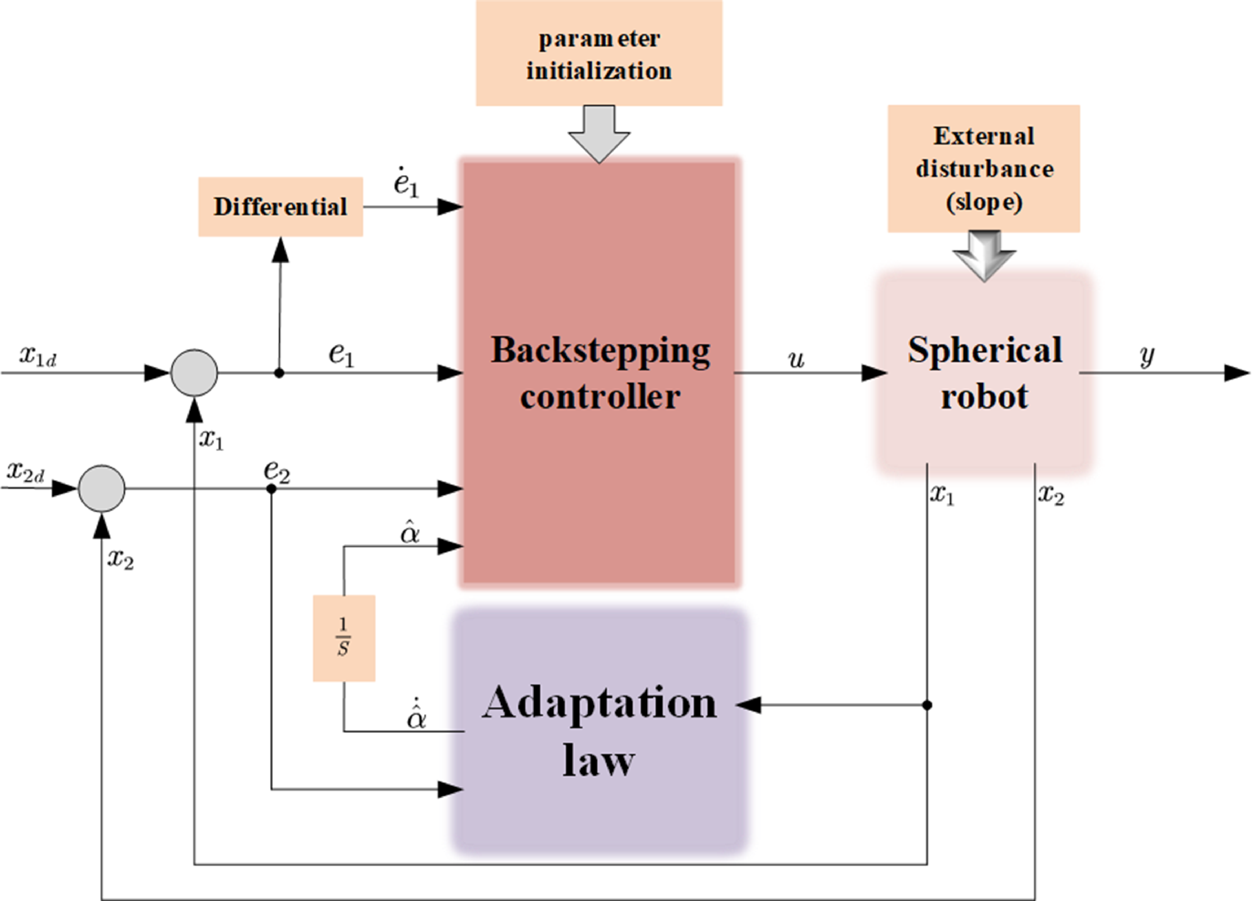
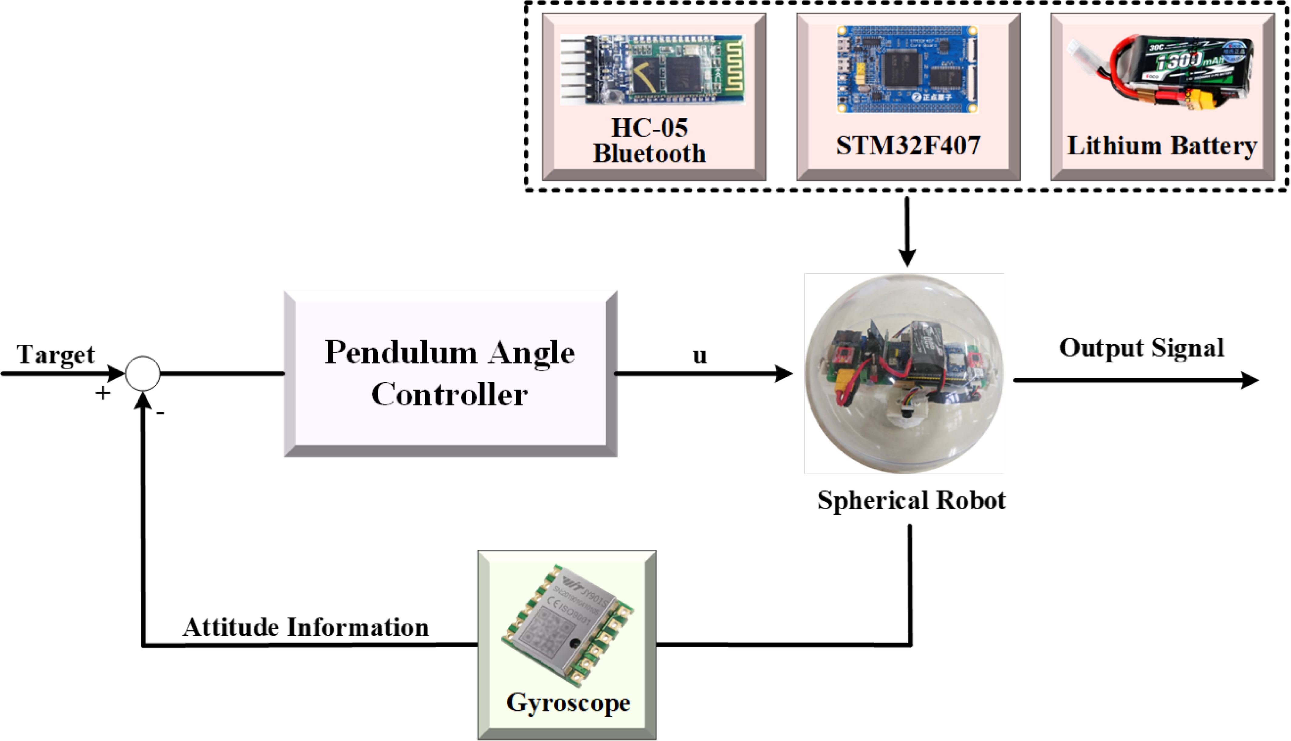
The overall control system of the spherical robot is shown in Figure 3.
4. Experiment
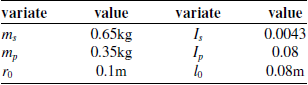
The impact of slopes on the movement of spherical robots is significant. We validate the climbing performance of the spherical robot through both simulation experiments and physical experiments. The simulation experiments assess the feasibility of the climbing control method for the spherical robot and its motion control under various conditions. The physical experiments confirm the applicability of the controller in real-world environments. The data pertaining to the spherical robot used in this study is presented in Table I.
Control block diagram.

Variable table.

4.1. Simulation experiment
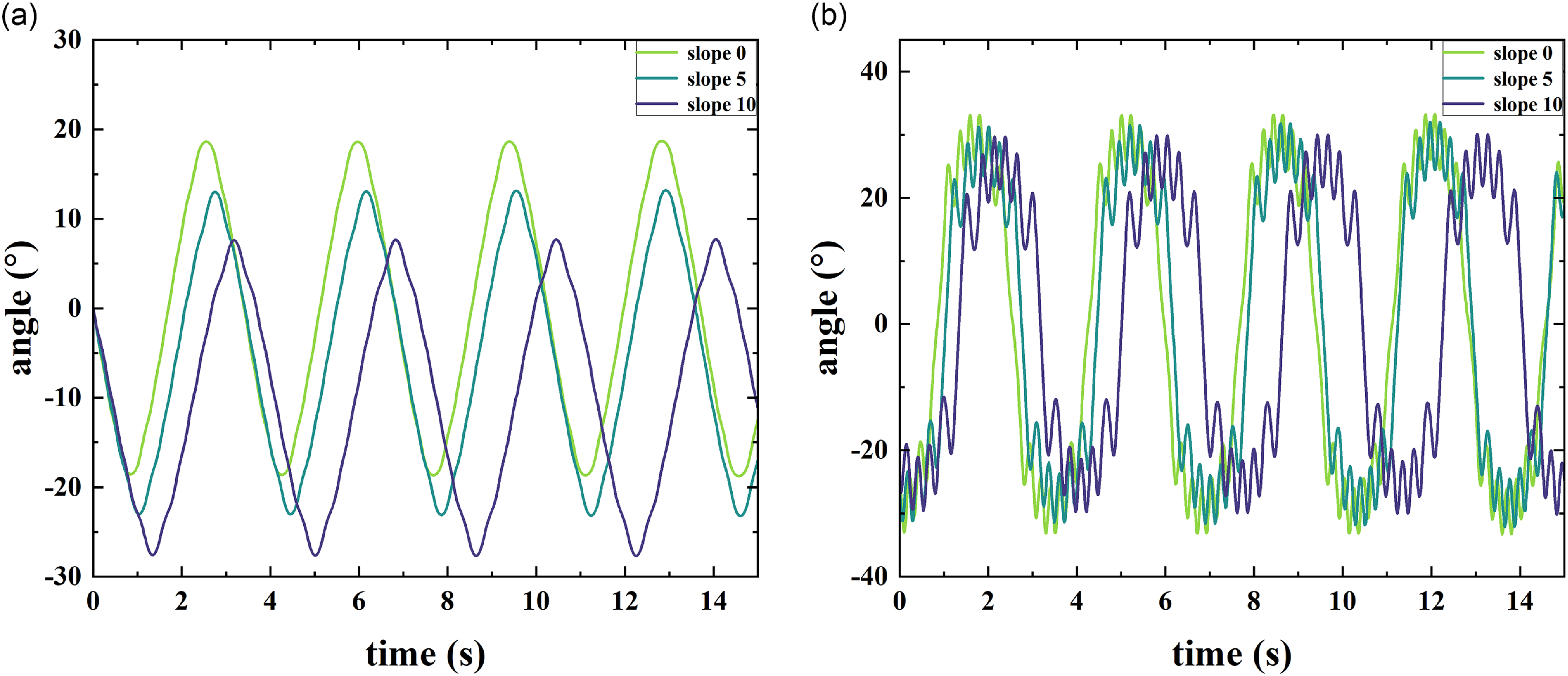
The spherical robot simulation experiment is divided into two parts, the first part is to verify the influence of slope on the angle variables inside the spherical robot.
In previous studies, it was found that different slope angles
 $\alpha$
have a negligible impact on the rotation angle
 $\varphi$
of the spherical robot’s shell and can be ignored. However, in the system, the slope angle
 $\alpha$
has a significant influence on the pendulum angle
 $\theta$
of the spherical robot. To verify this, we varied the slope angle
 $\alpha$
and observed its effect on the pendulum angle
 $\theta$
. As shown in Figure 4, changes in the slope angle
 $\alpha$
have a substantial impact on the pendulum angle
 $\theta$
of the spherical robot, while its effect on the pendulum angular velocity
 $\dot {\theta }$
is relatively minor.
Effects of different slopes on the overall system (a): impact on
 $x_1$
; (b): impact on
 $x_2$
.

In the second part, the influence of the slope angle
 $\alpha$
on the pendulum angle
 $x_1$
(
 $\theta$
) and its angular velocity
 $x_2$
(
 $\dot {\theta }$
) is considered. The state-space equation for the pendulum angle Eq. (17) is utilized in subsequent experiments. This paper analyzes the control performance of the pendulum angle
 $x_1$
of the spherical robot under varying slope conditions, including constant angle control and angle transition control.
Known Slope Conditions:
When the slope angle
 $\alpha$
is known, the control law given by Eq. (25) is employed for pendulum control. Figs. 5, 6, 7, and 8 demonstrate the performance of the proposed control system in tracking sinusoidal and constant reference signals for
 $x_1$
(pendulum angle
 $\theta$
) and
 $x_2$
(angular velocity
 $\dot {\theta }$
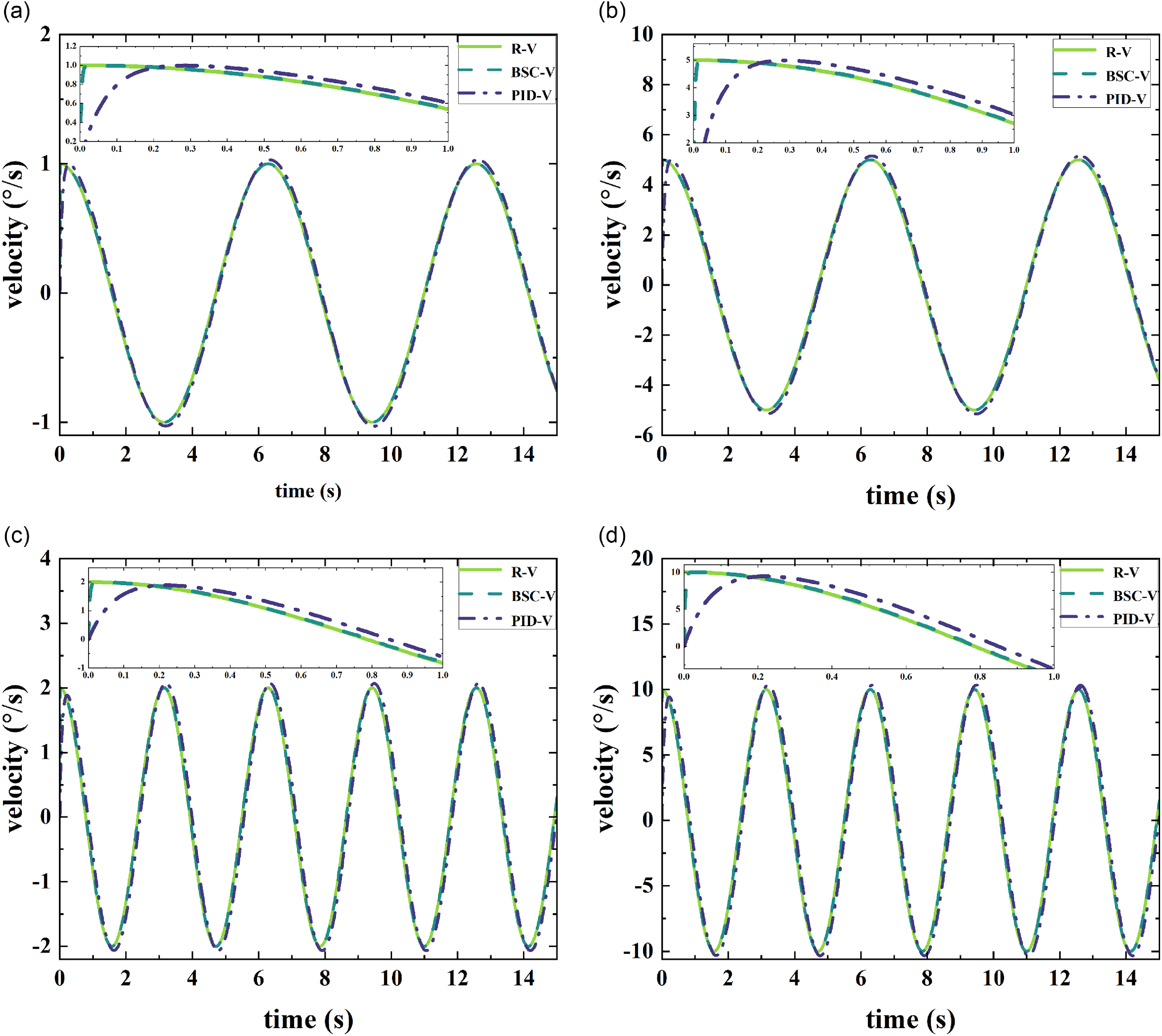
). In prior studies on spherical robots, the relationship between the pendulum angle and the shell angle was characterized by sinusoidal oscillations corresponding to linear growth, enabling uniform motion of the spherical robot. Therefore, in Figure 5, the reference value for
 $x_1$
is set to vary sinusoidally. The backstepping control method (BSC) is used to track sinusoidal signals of different frequencies for both the pendulum angle
 $x_1$
and the angular velocity
 $x_2$
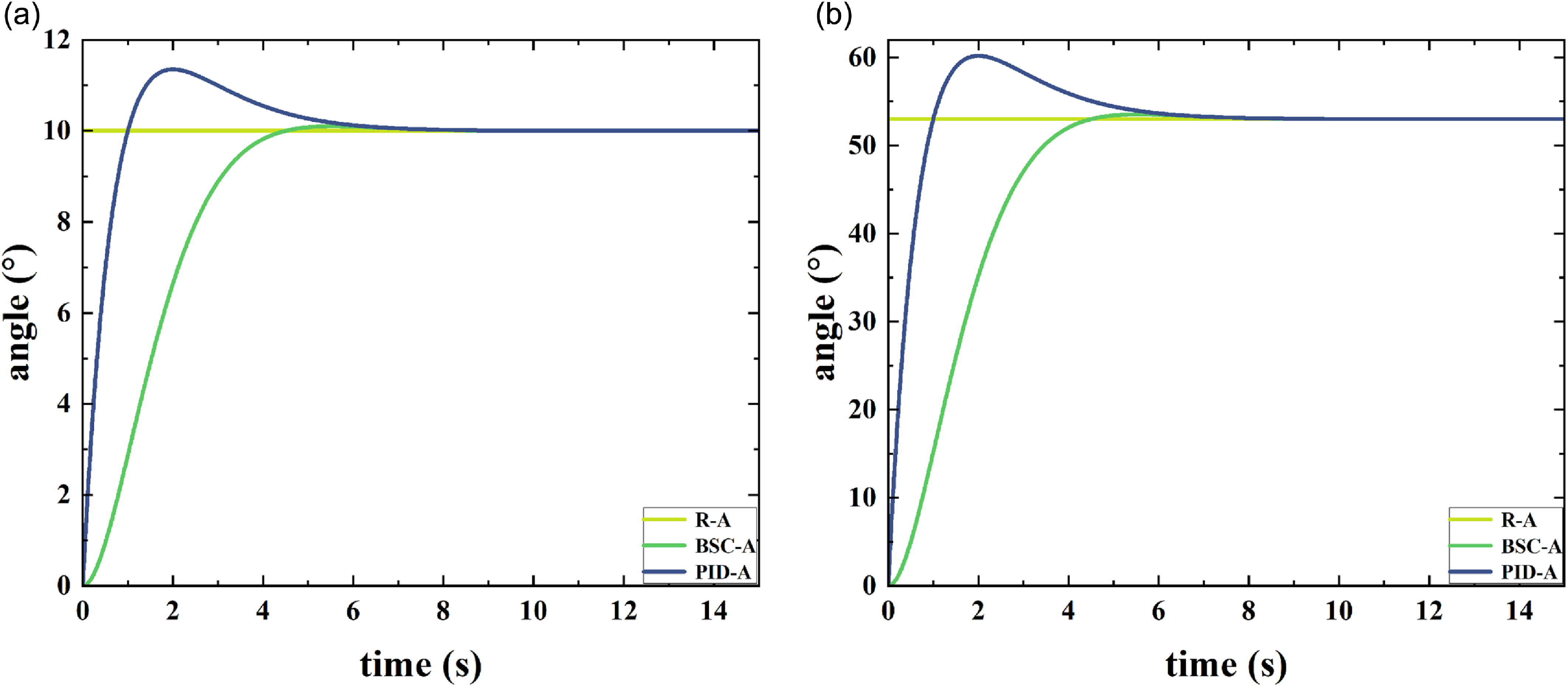
. In Figure 7, the backstepping control method is applied to track a constant reference signal, simulating the control of the pendulum at a fixed angle. This approach ensures the stability of the spherical robot on slopes of varying gradients in practical scenarios.
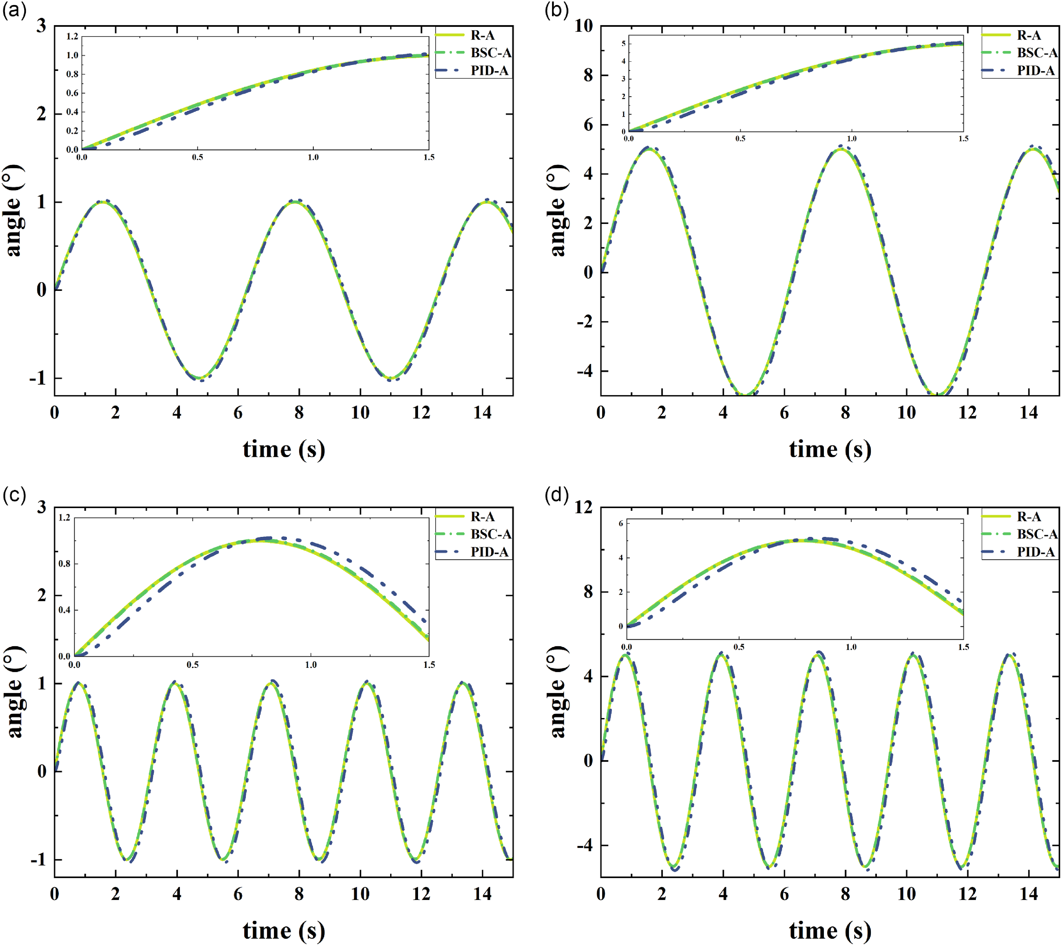
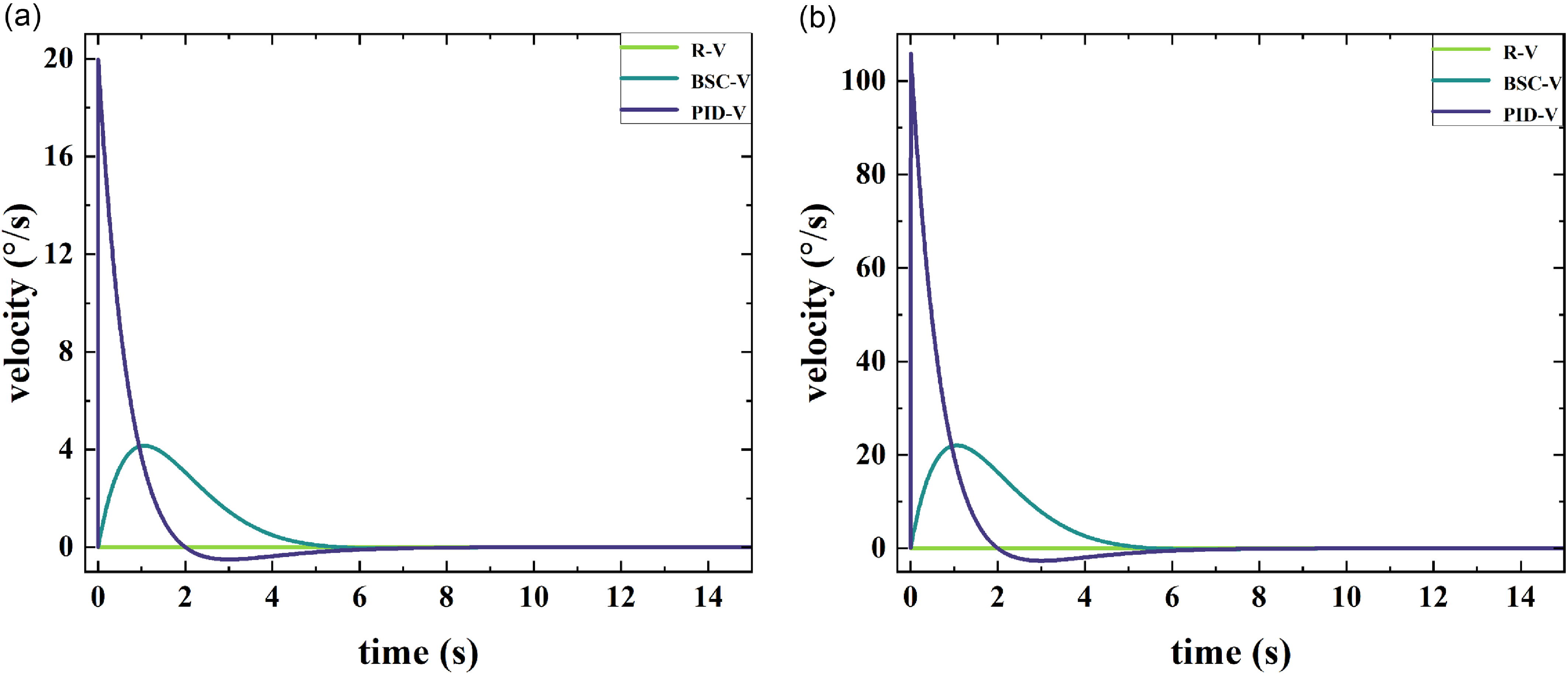
Figure 5 illustrates the control performance of the pendulum angle, while Figure 6 demonstrates the control of the angular velocity of the pendulum. In the experiments, the PID control was selected as a benchmark for comparison. During the motion of the spherical robot, the sinusoidal oscillation of the pendulum plays a crucial role in its locomotion. This paper investigates the tracking of sinusoidal signals with varying amplitudes and frequencies.
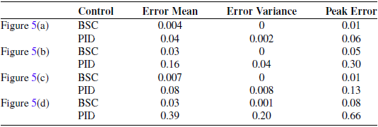
Tracking error data for the sinusoidal signals of
 $x_1$
.

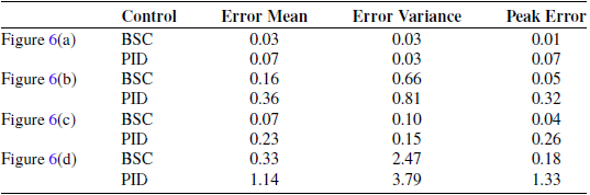
Tracking error data for the sinusoidal signals of
 $x_2$
.

The sinusoidal signal tracking control for
 $x_1$
is performed under the following conditions: (a) Tracking a signal with an amplitude of 1 and a frequency of
 $\frac {1}{2\pi }$
;(b) Tracking a signal with an amplitude of 5 and a frequency of
 $\frac {1}{2\pi }$
; (c) Tracking a signal with an amplitude of 1 and a frequency of
 $\frac {1}{\pi }$
; (d) Tracking a signal with an amplitude of 5 and a frequency of
 $\frac {1}{\pi }$
(R-A: reference angle; R-V: reference velocity; BSC: backstepping control).

The sinusoidal signal tracking control for
 $x_2$
is performed under the following conditions: (a) Tracking a signal with an amplitude of 1 and a frequency of
 $\frac {1}{2\pi }$
; (b) Tracking a signal with an amplitude of 5 and a frequency of
 $\frac {1}{2\pi }$
; (c) Tracking a signal with an amplitude of 1 and a frequency of
 $\frac {1}{\pi }$
; (d) Tracking a signal with an amplitude of 5 and a frequency of
 $\frac {1}{\pi }$
.

In Table III (corresponding to Figure 6), the peak error calculation excludes tracking errors during the initial phase (within 1 s) to ensure the accuracy of the results.
In the tracking curve comparison, the BSC (Backstepping Control) demonstrates significantly better tracking performance than PID control, with PID exhibiting noticeable tracking errors. Tables II and III present the tracking error data corresponding to Figs. 5 and 6.
Mean Error: For tracking
 $x_1$
, the mean error of BSC ranges from 0.004 to 0.03, while that of PID ranges from 0.04 to 0.39. This indicates that BSC provides more stable and precise control in terms of mean error. For tracking
 $x_2$
, the mean error of BSC ranges from 0.03 to 0.33, while that of PID ranges from 0.07 to 0.36. Again, BSC outperforms PID in mean error performance.
Variance: For tracking
 $x_1$
, the variance of BSC ranges from 0 to 0.001, while that of PID ranges from 0.002 to 0.20. This shows that BSC exhibits greater stability in error fluctuations. For tracking
 $x_2$
, the variance of BSC ranges from 0.03 to 2.47, while that of PID ranges from 0.03 to 3.79. Although BSC shows higher variance in some cases, it generally maintains better stability overall.
The constant signal tracking control for
 $x_1$
is performed under the following conditions: (a) A step signal with a value of 10; (b) A step signal with an amplitude of 53.

The constant signal tracking control for
 $x_2$
is performed under the following conditions: (a) A step signal with a value of 10; (b) A step signal with an amplitude of 53.

Peak Error: For tracking
 $x_1$
, the peak error of BSC ranges from 0.01 to 0.08, while that of PID ranges from 0.06 to 0.66. BSC demonstrates superior performance in peak error control. For tracking
 $x_2$
, the peak error of BSC ranges from 0.01 to 0.18, while that of PID ranges from 0.07 to 0.32. BSC also performs better in peak error control.
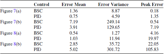
By analyzing Table IV, we obtain the following analysis.
Mean Error: For tracking
 $x_1$
, the mean error of BSC ranges from 1.36 to 7.19, while that of PID ranges from 0.75 to 3.91. In some cases, PID control performs better in terms of mean error. For tracking
 $x_2$
, the mean error of BSC ranges from 0.54 to 2.85, while that of PID ranges from 1.03 to 5.02. BSC demonstrates more stable and precise control in mean error performance.
Tracking error data for the constant signals of
 $x_1$
and
 $x_2$
.

Variance: For tracking
 $x_1$
, the variance of BSC ranges from 8.87 to 249.14, while that of PID ranges from 4.59 to 129.65. Due to the longer convergence time of BSC, PID control performs better in terms of variance. For tracking
 $x_2$
, the variance of BSC ranges from 1.27 to 35.72, while that of PID ranges from 11.94 to 301.72. BSC exhibits greater stability in variance performance.
Peak Error: For tracking
 $x_1$
, the peak error of BSC ranges from 0.18 to 0.54, while that of PID ranges from 1.35 to 7.19. BSC demonstrates superior performance in peak error control. For tracking
 $x_2$
, the peak error of BSC ranges from 4.16 to 22.05, while that of PID ranges from 19.97 to 105.83. BSC also performs better in peak error control.
Under known slope conditions, a comparison between BSC (Backstepping Control) and PID control was conducted. The data reveal that BSC outperforms PID in terms of mean error, variance, and peak error. This indicates that BSC exhibits superior robustness and precision when dealing with nonlinear systems and complex dynamics. In contrast, PID control performs poorly in handling high-frequency dynamics and nonlinear systems, particularly in peak error and variance, showing significant fluctuations and instability.
Unknown Slope Conditions:
When the slope angle
 $\alpha$
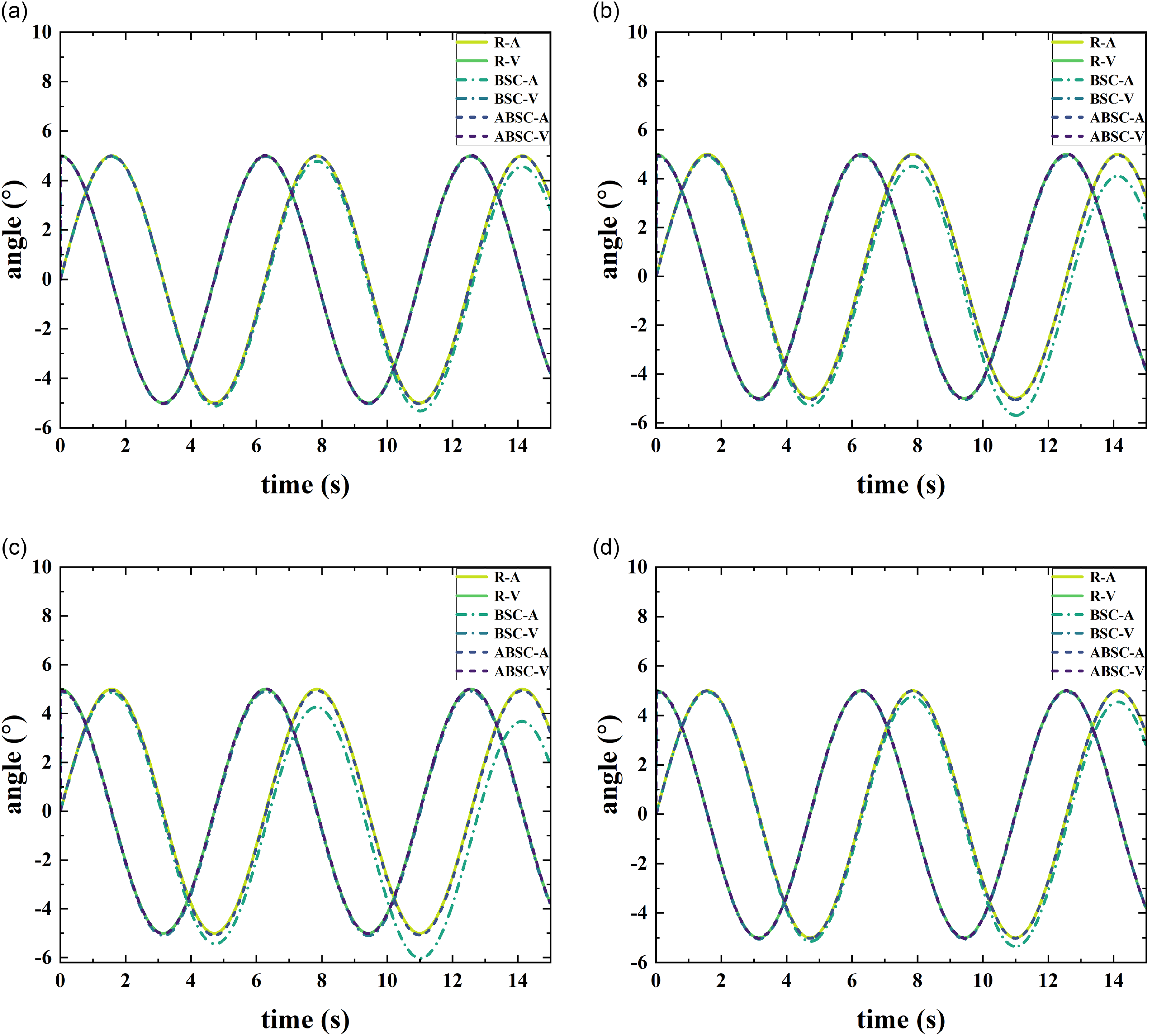
is unknown, it is treated as a dynamic disturbance with an unspecified value. In the control law, the slope is addressed through parameter estimation and compensation. The adaptation law of the slope parameter, given by Eq. (32), enables the estimation of the unknown slope. Figure 9 presents the experimental validation results.
Adaptive control of
 $x_1$
and
 $x_2$
(a) the slope is 5; (b) the slope is 10; (c) the slope of 15; (d) the slope is a random value; (ABSC: adapt backstepping control).

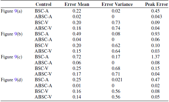
By analyzing Table V, we obtain the following analysis.
Mean Error: For pendulum angle control, the mean error of ABSC (Adaptive Backstepping Control) is significantly lower than that of BSC across all slope conditions. For example, at a slope of
 $5^\circ$
, the mean error of ABSC is 0.02, while that of BSC is 0.22. For pendulum angular velocity control, the mean error of ABSC is also generally lower than that of BSC, demonstrating superior tracking performance.
Variance: For pendulum angle control, the variance of ABSC is 0 (variance less than 0.001) under all slope conditions, indicating extremely high stability. In contrast, the variance of BSC ranges from 0.02 to 0.17. For pendulum angular velocity control, the variances of ABSC and BSC are similar, but ABSC-V performs better in terms of peak error.
Adaptive control error data for
 $x_1$
and
 $x_2$
.

Peak Error: For pendulum angle control, the peak error of ABSC is significantly lower than that of BSC across all slope conditions. For example, at a slope of
 $15^\circ$
, the peak error of ABSC is 0.08, while that of BSC is 1.37. For angular velocity control, the peak error of ABSC is also generally lower than that of BSC, demonstrating better extreme error control capability.
Precision and Stability: ABSC (Adaptive Backstepping Control) demonstrates excellent performance in mean error and peak error, exhibiting higher precision and stability.
Adaptive Capability: ABSC effectively adapts to varying slope conditions, showcasing superior robustness and adaptability.
Limitations of BSC: BSC (Backstepping Control) exhibits fluctuations and instability, particularly in handling different slope conditions. It performs poorly in extreme error control, with higher peak errors and significant variance, indicating greater fluctuations and instability.
Physical control block diagram of spherical robot.

4.2. Real experiment
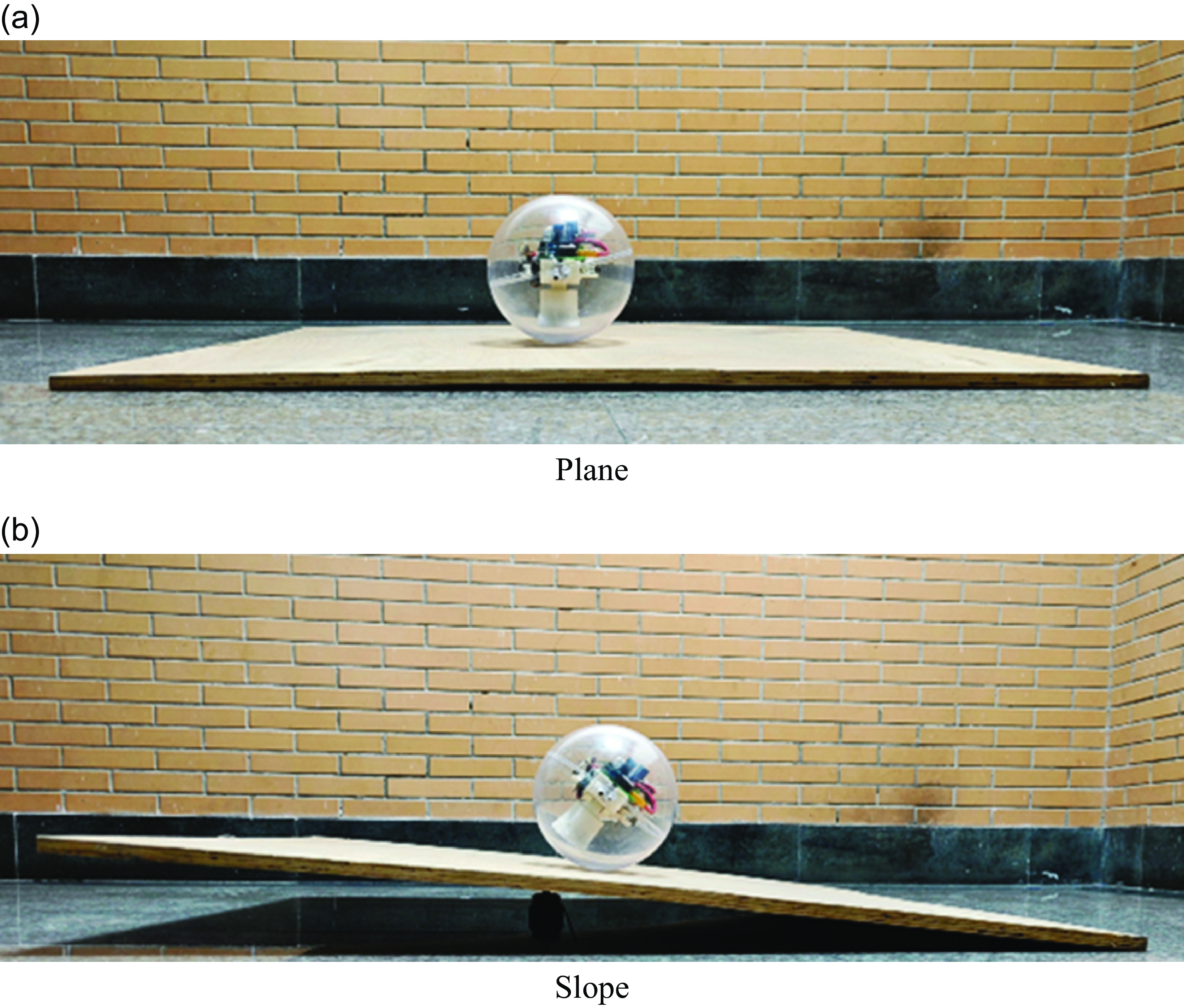
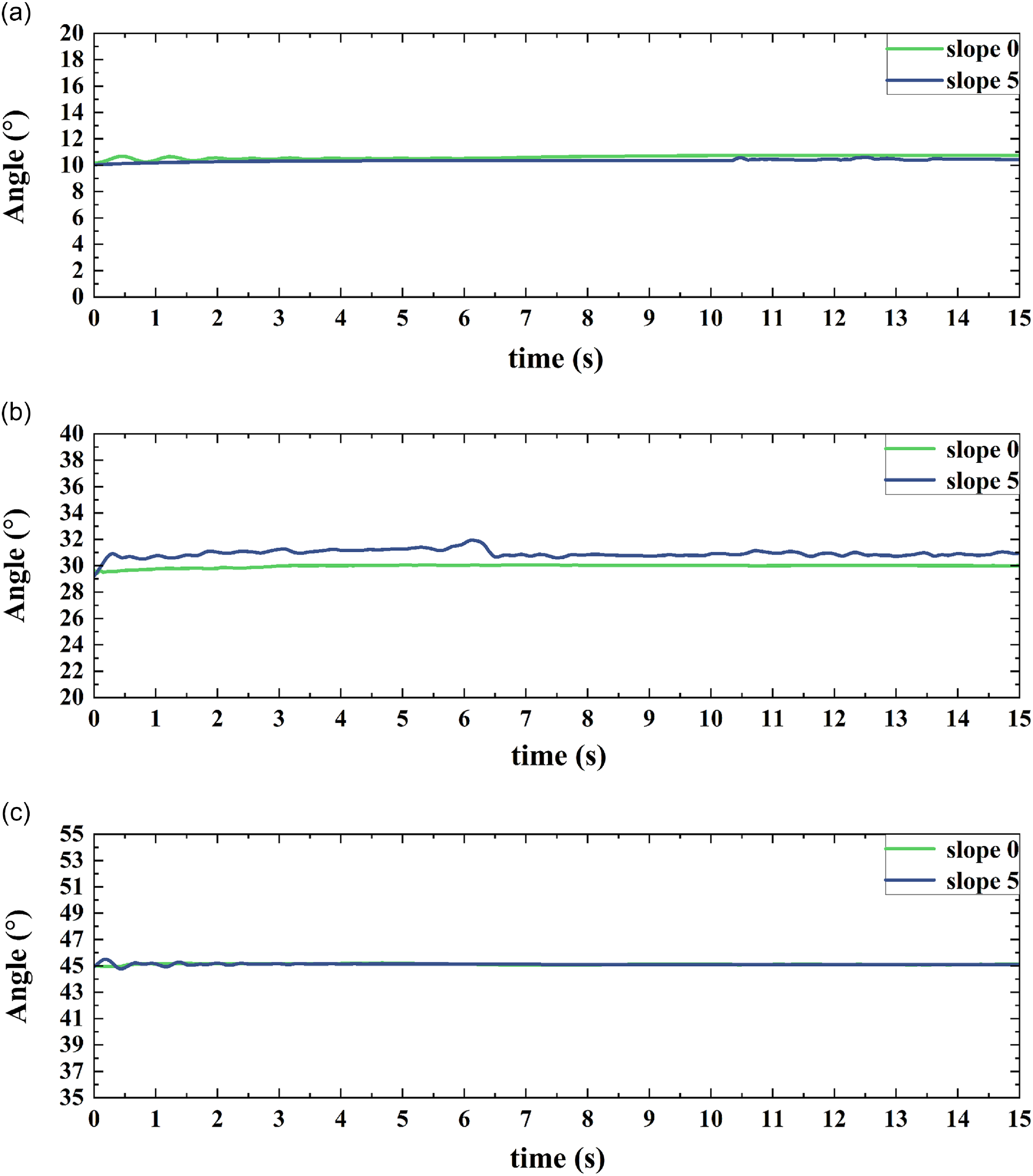
In the aspect of real experiment, this paper has carried on the experimental control of fixed Angle. The XK-I spherical robot experimental platform of the team was used to carry out specific experiments. The platform is shown in Figure 10. Figure 11 shows the motion experimental environment of the spherical robot.
The main control of XK-I spherical robot is stm32F407 series chip. In this paper, flat wooden boards are used to build the slope environment required by the experiment. The board has enough friction. Among them, the slope in Figure 11(b) is
 $5^{\circ }$
.
Spherical robot experiment environment.

Different angle control for
 $x_1$
(a) The control angle is
 $10^{\circ }$
; (b) The control angle is
 $30^{\circ }$
; (c) The control angle is
 $45^{\circ }$
.

In Figure 12, tests were carried out in the environment of slope 0 and slope
 $5^{\circ }$
respectively. In the existing environment, the slope requirements of most roads and other environments are less than
 $10^{\circ }$
. Therefore, the test was conducted in an environment with a slope of
 $5^{\circ }$
. When the pendulum Angle
 $x_1$
is
 $10^{\circ }$
, the control effect is relatively stable under both slope conditions. When the control Angle is
 $30^{\circ }$
, there are some fluctuations. When the control Angle is
 $45^{\circ }$
, it tends to be stable. When the slope is
 $5^{\circ }$
, the actual balance Angle of the spherical robot is about
 $30^{\circ } \sim 40^{\circ }$
, so when controlling the balance state, the control of the spherical robot is more difficult and the fluctuation is greater.
5. Conclusion
This study focuses on the analysis and control of spherical robots during slope-climbing motion. Through kinematic modeling, simulation, and physical experiments, the slope-climbing behavior of spherical robots was investigated and analyzed. Under known slope conditions, the Backstepping Control (BSC) algorithm effectively controls the pendulum angle (
 $x_1$
and
 $x_2$
), demonstrating low mean error, variance, and peak error. These results validate its superiority in terms of stability and precision. Under unknown slope conditions, the Adaptive Backstepping Control (ABSC) algorithm exhibits stronger robustness, effectively mitigating the impact of external disturbances and uncertainties. It significantly reduces tracking error and fluctuations, particularly excelling in peak error control. The control system performs reliably on slopes of
 $0^\circ$
and
 $5^\circ$
, and experiments confirm that both BSC and ABSC algorithms achieve stable control in typical environments with slopes less than
 $10^\circ$
. The feasibility of the BSC and ABSC algorithms has been verified across various motion states, particularly their effectiveness under different slope conditions. Physical experiments further demonstrate the applicability of these algorithms to real-world prototypes, providing theoretical support and technical assurance for the practical deployment of spherical robots in complex terrains, such as undulating surfaces and slopes.
Author contributions
Jianwen Huo, Rui Lin, and Tujiu Li conceived and designed the study. Rui Lin carried out the simulation and physical verification of the robot. Rui Lin, Qiguan Wang, and Tujiu Li conducted data gathering and performed statistical analyses. Rui Lin and Jianwen Huo wrote the article.
Financial support
Supported by Postgraduate Innovation Fund Project by Southwest University of Science and Technology (24ycx2017).
Competing interests
The authors declare no conflicts of interest exist.
Ethical approval
Not applicable.