





1. Introduction
Over the last few years, there have been many studies carried out in deciphering the impact of an odd viscosity in classical fluids since the seminal work of Avron (Reference Avron1998). As discussed by Avron, if the time-reversal symmetry of the viscous fluid is broken either spontaneously or by external fields, the non-dissipative effect of the odd viscosity coefficient needs to be taken care of along with the dissipative effect of the even viscosity coefficient. He reported that the time-reversal symmetry for the superfluid He $^3$ is broken spontaneously, while the time-reversal symmetry for the two-dimensional quantum Hall fluid is broken in the presence of an external magnetic field. As a result, the odd viscosity component does not vanish; rather, it provides an off-diagonal contribution to the Cauchy stress tensor. Hence, the modified Navier–Stokes equations are required to describe the motion of a fluid endowed with an odd viscosity coefficient, which is expected to play a significant role in the complex wave dynamics of such fluids.
In this context, Lapa & Hughes (Reference Lapa and Hughes2014) initiated the study of nearly circular swimmers in two-dimensional fluids with odd viscosity at low Reynolds number. It was shown that the non-vanishing odd viscosity component contributes to the hydrodynamic stress tensor and plays a major role in swimming strategies. The effect of odd viscosity in chiral active fluids was examined by Banerjee et al. (Reference Banerjee, Souslov, Abanov and Vitelli2017) due to the broken time-reversal symmetry in their non-equilibrium steady states. On the other hand, the effect of an odd viscosity in two-dimensional incompressible fluids was explored by Ganeshan & Abanov (Reference Ganeshan and Abanov2017) to examine the bubble dynamics in a planar Stokes flow with stress-free boundary conditions. It was predicted that the shape of the bubble is explicitly dependent on the odd viscosity coefficient. The effect of odd viscosity on the free surface flow of a colloidal chiral fluid was explored experimentally by Soni et al. (Reference Soni, Bililign, Magkiriadou, Sacanna, Bartolo, Shelley and Irvine2019), where a millimetre-scale cohesive chiral fluid flow was created by spinning millions of colloidal magnets under a magnetic field. They demonstrated that the macroscopic chiral fluid flow has a resemblance to the free surface flow of Newtonian fluids. Furthermore, they showed that thin streams of chiral fluid become unstable as observed on the surface of a fluid flowing past a solid object. Recently, the effect of the odd viscosity has been investigated by Kirkinis & Andreev (Reference Kirkinis and Andreev2019) for a thin incompressible liquid film flow with broken time-reversal symmetry. Basically, they deciphered the influence of the odd viscosity on the thermocapillary instability for thin liquid films sitting on a heated solid substrate. As discussed by Kirkinis & Andreev (Reference Kirkinis and Andreev2019), the waves induced by the thermocapillary effect can be suppressed by the odd viscosity coefficient. Later, the effect of an odd viscosity on the stability of a falling film was analysed by Zhao & Jian (Reference Zhao and Jian2021a) in the presence of an electromagnetic field. The instability analysis was performed under the framework of the Benney-type surface evolution equation in terms of the local film thickness. It was reported that both the odd viscosity and magnetic field stabilize the surface instability. Weakly nonlinear analysis was also performed, which revealed that the supercritical stable region is reduced by the odd viscosity coefficient. Zhao & Jian (Reference Zhao and Jian2021b) further performed a similar analysis for a viscoelastic liquid (Walters’ liquid  $B''$), where it was assumed that the viscoelastic liquid has a property of broken time-reversal symmetry. They mentioned that viscoelasticity destabilizes the surface instability. However, the surface instability is stabilized by the odd viscosity through the increase of the critical Reynolds number. The study proposed by Zhao & Jian (Reference Zhao and Jian2021a) was further revisited by Chattopadhyay (Reference Chattopadhyay2021) and Mukhopadhyay & Mukhopadhyay (Reference Mukhopadhyay and Mukhopadhyay2021) in the presence of a slippery plane based on the Benney-type surface evolution equation valid in the vicinity of the critical Reynolds number for the surface mode. However, the effect of the electromagnetic field was not included in their studies. Again, the stabilizing influence of the odd viscosity on the surface mode was reported. A weakly nonlinear analysis was also carried out, and the shrinking of the supercritical stable region was found. Obviously, the above studies regarding thin film flows endowed with an odd viscosity coefficient were confined to the vicinity of the threshold of instability. In addition, the experimental study of Soni et al. (Reference Soni, Bililign, Magkiriadou, Sacanna, Bartolo, Shelley and Irvine2019) based on a chiral fluid demonstrated some familiar features of free surface flows such as droplets merging, spreading of fluid under the influence of gravity and instability of thin streams. These facts motivate us to investigate the thin film instability in detail for incompressible fluids with broken time-reversal symmetry. The effect of the magnetic field is not incorporated in the current study.
The purpose of the present study is to explore the effect of an odd viscosity on the surface wave and shear wave dynamics for a viscous incompressible fluid endowed with an odd viscosity coefficient flowing down an inclined plane, not only in the low Reynolds number regime but also in the high Reynolds number regime. In particular, the surface wave appears in the low Reynolds number regime and evolves downstream when the Reynolds number exceeds the critical value  $(5/4) \cot \theta$, where
 $\theta$ is the inclination angle with the horizontal (Benjamin Reference Benjamin1957; Yih Reference Yih1963). On the other hand, the shear wave appears only in the high Reynolds number regime when the inclination angle is sufficiently small. Furthermore, such waves compete with each other to trigger the primary instability of base flow/parallel flow with a flat surface at a low value of inclination angle (Lin Reference Lin1967; Bruin Reference Bruin1974). In order to study the linear dynamics of such waves, the Orr–Sommerfeld eigenvalue problem is derived, while to deal with the nonlinear wave dynamics, the two-equation depth-averaged model is derived in terms of the local fluid layer thickness and local flow rate. The numerical solution of the Orr–Sommerfeld eigenvalue problem renders two dominant modes, the so-called surface mode and shear mode, which can be stabilized by the odd viscosity. In fact, the surface wave is generated by the surface mode responsible for the streamwise component of the gravitational force, while the shear wave is generated by the shear mode responsible for the viscous force (Chin, Abernath & Bertschy Reference Chin, Abernath and Bertschy1986). The interesting result is that the surface mode dominates the primary instability of the base flow at a low viscosity ratio of odd viscosity coefficient to even viscosity coefficient. But there exists an unstable range of finite wavenumber where the shear mode dominates the primary instability of the base flow at a high viscosity ratio when the Reynolds number is large. On the other hand, the numerical solution of the two-equation model predicts that both the maximum amplitude and speed of the steady state travelling wave solution decrease in the presence of an odd viscosity coefficient. In addition, the odd viscosity coefficient significantly delays the transition from the primary sinusoidal-type periodic waves to secondary solitary-type waves developed through a sequence of nonlinear wave interactions downstream.
2. Mathematical formulation
Suppose a two-dimensional incompressible viscous fluid with thickness  $h(x,t)$ flowing down an inclined plane with angle
 $\theta$ subject to the gravitational force
 $g$, as shown schematically in figure 1. The Cartesian coordinate frame is selected to describe the fluid motion, where the origin is located in the inclined plane, and
 $x$ and
 $y$ axes are placed in streamwise and cross-stream directions, respectively. Here,
 $h_N$ is the thickness of the undeformed fluid surface indicated by the dashed line, and
 $h(x,t)$ is the thickness of the deformed fluid surface. We assume that the viscous fluid has a property with broken time-reversal symmetry that introduces an additional viscosity coefficient, termed the odd viscosity or Hall viscosity coefficient, to the Cauchy stress tensor. Such a non-dissipative effect of the viscosity tensor was found in quantum Hall fluids at zero temperature (Ganeshan & Abanov Reference Ganeshan and Abanov2017). In fact, the time-reversal symmetry of a viscous fluid can be broken either spontaneously or in the presence of an external magnetic field (Avron Reference Avron1998). In general, the stress tensor
 $\tau _{ij}$ of a viscous fluid can be represented in terms of the rate of strain tensor
 $\partial _{x_l}u_{k}$ as (Landau & Lifshitz Reference Landau and Lifshitz1959)
Schematic diagram of a falling viscous fluid with an odd viscosity coefficient. Here,  $h_N$ is the thickness of the undeformed fluid surface indicated by the dashed line, and
 $h(x,t)$ is the thickness of the deformed fluid surface.

 \begin{equation} \tau_{ij}={-}p \delta_{ij}+\mu_{ijkl} \partial_{x_l}u_{k}, \end{equation}
where  $\mu _{ijkl}$ is the viscosity tensor of rank
 $4$ and p is the pressure of the fluid. Conservation of angular momentum implies that the stress tensor is symmetric under the exchange of its two indices
 $i$ and
 $j$ if the net external torque vanishes. However, if the first and last pairs of indices are exchanged, i.e. if
 $(ijkl) \to (klij)$, the viscosity tensor is divided into symmetric (even) and antisymmetric (odd) parts (Avron, Seller & Zograf Reference Avron, Seller and Zograf1995), where
 \begin{equation} \mu^e_{ijkl}=\mu^e_{klij}, \quad \mu^o_{ijkl}={-}\mu^o_{klij}. \end{equation}
The antisymmetric part associated with the non-dissipative effect vanishes with the aid of the Onsager reciprocal relation  $L_{\alpha \beta }=L_{\beta \alpha }$ (where
 $\alpha =ij$ and
 $\beta =kl$) if time-reversal symmetry holds (Onsager Reference Onsager1931), where
 $L_{\alpha \beta }$ represents any linear transport coefficient. However, for an isotropic fluid with broken time-reversal symmetry, the antisymmetric part is non-zero, and thereby, the Cauchy stress tensor
 $\tau _{ij}$ will have two components rather than one
 \begin{equation} \tau_{ij}=\tau^e_{ij}+\tau^o_{ij}, \end{equation}
where  $\tau ^e$ and
 $\tau ^o$, respectively, represent the even and odd components of the Cauchy stress tensor. The even component of the Cauchy stress tensor has a conventional form (Landau & Lifshitz Reference Landau and Lifshitz1959; Batchelor Reference Batchelor1993; Oron, Davis & Bankoff Reference Oron, Davis and Bankoff1997)
 \begin{equation} \tau^e_{ij}={-}p \delta_{ij}+\mu^e(\partial_{x_i}u_j+\partial_{x_j}u_i),\quad {\rm where}\ i,j=1,2, \end{equation}
where  $u_i$ and
 $u_j$ are velocity components of the fluid,
 $\mu ^e$ is the standard/even viscosity coefficient and
 $\delta _{ij}$ is the Kronecker delta. On the other hand, the odd component of the Cauchy stress tensor can be expressed as (Avron Reference Avron1998; Lapa & Hughes Reference Lapa and Hughes2014; Kirkinis & Andreev Reference Kirkinis and Andreev2019)
 \begin{equation} \tau^o_{ij}={-}\mu^o(\delta_{i1}\delta_{j1}-\delta_{i2} \delta_{j2})(\partial_{x_2}u_1+\partial_{x_1}u_2)+\mu^o(\delta_{i1}\delta_{j2} +\delta_{i2}\delta_{j1})(\partial_{x_1}u_1-\partial_{x_2}u_2), \end{equation}
where  $i,j=1,2$ and
 $\mu ^o$ is the odd viscosity coefficient. For the sake of simplicity, we assume
 $u_1=u$,
 $v_1=v$,
 $x_1=x$ and
 $x_2=y$. In what follows, we can show that
 \begin{equation} \tau^o_{xy}=\mu^o(\partial_xu-\partial_yv)=\tau^o_{yx}, \quad \tau^0_{xx}={-}\mu^o(\partial_yu+\partial_xv), \quad \tau^o_{yy}=\mu^o(\partial_yu+\partial_xv). \end{equation}
Obviously, the odd component of the Cauchy stress tensor also maintains the symmetric property as manifested in the even component. Since the viscous fluid considered in the present study has a property with broken time-reversal symmetry, the two-dimensional fluid flow is governed by the modified Navier–Stokes equations (Kirkinis & Andreev Reference Kirkinis and Andreev2019)
 \begin{gather} \partial_xu+\partial_yv=0, \end{gather}
 \begin{gather}\rho(\partial_tu+u\partial_xu+v\partial_yu)={-}\partial_xp+\mu^e(\partial_{xx}u+ \partial_{yy}u)-\mu^o(\partial_{xx}v+\partial_{yy}v)+\rho g \sin \theta, \end{gather}
 \begin{gather}\rho(\partial_tv+u\partial_xv+v\partial_yv)={-}\partial_yp+\mu^e(\partial_{xx}v+ \partial_{yy}v)+\mu^o(\partial_{xx}u+\partial_{yy}u)-\rho g \cos \theta. \end{gather}
It should be noted that extra viscous terms appear in the momentum equations due to the presence of an odd viscosity coefficient. The above governing equations are subjected to the following boundary conditions. At the inclined plane,  $y=0$, fluid velocity components must satisfy no-slip and no-penetration boundary conditions
 \begin{equation} u=0, \quad v=0. \end{equation}
At the fluid surface,  $y=h(x,t)$, hydrodynamic stresses of the fluid must satisfy tangential stress and normal stress boundary conditions (see, for example Kirkinis & Andreev Reference Kirkinis and Andreev2019; Zhao & Jian Reference Zhao and Jian2021a,Reference Zhao and Jianb)
 \begin{gather} \tau_{ij}n_jt_i=0, \quad i,j=1,2, \end{gather}
 \begin{gather}\tau_{ij}n_in_j=\sigma \partial_{xx}h/[1+(\partial_xh)^2]^{3/2}, \quad i,j=1,2, \end{gather}
where  $\sigma$ is the surface tension,
 $(t_1, t_2)=(1, \partial _xh)/\sqrt {1+(\partial _xh)^2}$ is the direction cosine of the unit tangent vector
 $\boldsymbol {\hat {t}}$ and
 $(n_1, n_2)=(-\partial _xh,1)/\sqrt {1+(\partial _xh)^2}$ is the direction cosine of the unit normal vector
 $\boldsymbol {\hat {n}}$, placed on the fluid surface. Using the components of the Cauchy stress tensor, tangential stress and normal stress boundary conditions at the fluid surface,
 $y=h(x,t)$, can be read as
 \begin{align} &\frac{\mu^e}{[1+(\partial_xh)^2]}[2(\partial_yv-\partial_xu)\partial_xh+(\partial_yu+\partial_xv)\{1-(\partial_xh)^2\}]\nonumber\\ &\quad + \frac{\mu^o}{[1+(\partial_xh)^2]}[2(\partial_yu+\partial_xv)\partial_xh+(\partial_xu-\partial_yv)\{1-(\partial_xh)^2\}]=0, \end{align}
 \begin{align} &p_a-p+\frac{2\mu^e}{[1+(\partial_xh)^2]}[\partial_xu(\partial_xh)^2-(\partial_yu+\partial_xv)\partial_xh+\partial_yv] - \sigma \frac{\partial_{xx}h}{[1+(\partial_xh)^2]^{3/2}}\nonumber\\ &\quad +\frac{\mu^o}{[1+(\partial_xh)^2]}[(\partial_yu+\partial_xv)\{1-(\partial_xh)^2\}-2\partial_xh(\partial_xu-\partial_yv)]=0, \end{align}
where  $p_a$ is the ambient pressure. Finally, the kinematics of the fluid surface,
 $y=h(x,t)$, is governed by the kinematic boundary condition
 \begin{equation} \partial_{t}h+u\partial_{x}h =v. \end{equation}
As we are interested in inspecting the primary instability of base flow/parallel flow with a flat surface, it is essential to determine the exact solution of the base flow equations. As a consequence, we consider a uni-directional parallel flow with a constant fluid layer height. This assumption converts the deformed fluid surface into a flat undeformed fluid surface, i.e.  $y=h(x,t)=h_N$, and supplies a simplified set of governing equations for the base flow
 \begin{gather} \mu^e \partial_{yy}u+\rho g \sin \theta =0, \quad -\partial_yp+\mu^o\partial_{yy}u -\rho g \cos \theta=0, \end{gather}
 \begin{gather}u=0, \ {\rm at}\ y=0, \quad \mu^e\partial_yu=0, \quad p_a-p+\mu^o\partial_yu=0, \ {\rm at}\ y=h_N. \end{gather}
Here, we prefer the surface velocity of the base flow,  $U_s=\rho g h_N^2\sin \theta /(2\mu _e)$, as the characteristic velocity scale, the constant fluid layer height of the base flow,
 $h_N$, as the characteristic length scale,
 $\mu _e U_s/h_N$ as the characteristic pressure scale and
 $h_N/U_s$ as the characteristic time scale. Therefore, we can write
 \begin{equation} \left. \begin{array}{c@{}} x^*=x/h_N, \quad y^*=y/h_N, \quad h^*=h/h_N, \quad u^*=u/U_s, \\ v^*=v/U_s, \quad t^*=t/(h_N/U_s), \quad p^*=p/(\mu_e U_s/h_N), \end{array} \right\} \end{equation}
where the star variables indicate the non-dimensional variables. For the sake of simplicity, the star notation is dropped from the non-dimensional variables in the subsequent mathematical formulation. The exact solution of the base flow equations (2.16a,b) and (2.17a–c) in non-dimensional form can be expressed as follows:
 \begin{equation} U(y)=(2y-y^2), \quad P(y)=P_a+2(\mu+\cot\theta)(1-y), \quad V=0, \end{equation}
where  $P_a$ is the non-dimensional ambient pressure and
 $\mu =\mu ^o/\mu ^e$ is the ratio of the odd viscosity coefficient to the even viscosity coefficient, which will be later referred to as the viscosity ratio. It should be noted that the streamwise base velocity
 $U(y)$ is independent of the viscosity ratio
 $\mu$. However, the basic pressure
 $P(y)$ is explicitly dependent on the viscosity ratio
 $\mu$.
3. Linear stability analysis in the long-wave regime
In this section, we shall perform a linear stability analysis in the long-wave regime. To this end, an infinitesimal disturbance is applied to the base flow. This fact is mathematically expressed by the following flow variable decomposition:
 \begin{equation} \left. \begin{array}{c@{}} u(x,y,t)=U(y)+u'(x,y,t),\\ v(x,y,t)=v'(x,y,t),\\ p(x,y,t)=P(y)+p'(x,y,t),\\ h(x,t)=1+h'(x,t), \end{array} \right\} \end{equation}
where  $u'(x,y,t)$,
 $v'(x,y,t)$,
 $p'(x,y,t)$ and
 $h'(x,t)$ represent the perturbation velocity components, perturbation pressure and perturbation surface deformation, respectively. After substitution of the variable decomposition (3.1) in non-dimensional form into the governing equations (2.7)–(2.15) and linearization about the base flow solution, one can obtain the following non-dimensional perturbation equations:
 \begin{gather} \partial_xu'+\partial_yv'=0, \end{gather}
 \begin{gather}Re(\partial_tu' + U\partial_xu'+v'\partial_yU)+\partial_xp' -(\partial_{xx}u'+\partial_{yy}u')+\mu(\partial_{xx}v'+\partial_{yy}v')=0, \end{gather}
 \begin{gather}Re(\partial_tv'+U\partial_xv')+\partial_yp'-(\partial_{xx}v'+\partial_{yy}v') -\mu(\partial_{xx}u'+\partial_{yy}u')=0, \end{gather}
where  $Re=\rho U_s h_N/\mu ^e$, the Reynolds number, compares inertia with the viscous force. At the inclined plane,
 $y=0$, the linearized forms of no-slip and no-penetration boundary conditions are
 \begin{equation} u'=0, \quad v'=0. \end{equation}
On the other hand, at the fluid surface,  $y=1$, the boundary conditions can be linearized as
 \begin{gather} \partial_yu' + \partial_xv'+h'\partial_{yy}U +\mu (\partial_xu'-\partial_yv')=0, \end{gather}
 \begin{gather}-p'+2 (\mu+\cot \theta) h'+ 2\partial_yv'+\mu(\partial_yu' + \partial_xv'+h'\partial_{yy}U)-(1/Ca) \partial_{xx}h'=0, \end{gather}
 \begin{gather}\partial_th'+U\partial_x h'-v'=0, \end{gather}
where  $Ca=\mu ^eU_s/\sigma$, the capillary number compares the viscous force with the capillary force. Next, we assume the solution of the perturbation equations (3.2)–(3.8) in the form of the normal mode (Yih Reference Yih1963; Samanta Reference Samanta2020)
 \begin{equation} \left. \begin{array}{c@{}} u'(x,y,t)=\tilde{u}(y)\exp[{\rm i} k(x-ct)]+{\rm c.c.},\\ v'(x,y,t)=\tilde{v}(y)\exp[{\rm i} k(x-ct)]+{\rm c.c.},\\ p'(x,y,t)=\tilde{p}(y)\exp[{\rm i} k(x-ct)]+{\rm c.c.},\\ h'(x,t)=\tilde{h}\exp[{\rm i} k(x-ct)]+{\rm c.c.}, \end{array} \right\} \end{equation}
where  $\textrm {c.c.}$ represents the complex conjugate and the variables with the tilde notation represent the amplitudes of perturbation variables. Here,
 $k$ and
 $c$ are respectively the real wavenumber and complex wave speed of the infinitesimal perturbation because we are interested in figuring out the temporal stability analysis. Next, we introduce the perturbation streamfunction
 $\psi '(x,y,t)$ by using the relations
 $u'=\partial _y\psi '$ and
 $v'=-\partial _x\psi '$. After substitution of the normal mode form (3.9) into the perturbation equations (3.2)–(3.8) and eliminating pressure terms, one can obtain the Orr–Sommerfeld eigenvalue problem for the falling viscous fluid with broken time-reversal symmetry
 \begin{gather} (\partial_{yyyy}\tilde{\psi}-2k^2\partial_{yy}\tilde{\psi}+k^4\tilde{\psi}) -{\rm i}k Re[(U-c)(\partial_{yy}\tilde{\psi}-k^2\tilde{\psi})- \partial_{yy}U\tilde{\psi}]=0, \quad 0 \le y \le 1, \end{gather}
 \begin{gather}\tilde{\psi}=0, \quad \partial_y\tilde{\psi}=0, \text{ at } y=0, \end{gather}
 \begin{gather}\partial_{yy}\tilde{\psi}+k^2\tilde{\psi}+\tilde{h}\partial_{yy}U+2\, {\rm i} k\mu \partial_y\tilde{\psi}=0, \ {\rm at}\ y=1, \end{gather}
 \begin{gather}(\partial_{yyy}\tilde{\psi}-3k^2\partial_y\tilde{\psi})-{\rm i} k Re(U-c)\partial_y\tilde{\psi}-2\,{\rm i} k^3\mu\tilde{\psi}-{\rm i} k\tilde{h}[2\cot\theta+k^2/Ca]=0,\ {\rm at}\ y=1, \end{gather}
 \begin{gather}(U-c)\tilde{h}+\tilde{\psi}=0, \ {\rm at}\ y=1, \end{gather}
where  $\tilde {\psi }$ is the amplitude of the perturbation streamfunction.
3.1. Long-wave asymptotic solution
In accordance with the study of Yih (Reference Yih1963), the long-wave asymptotic solution of the Orr–Sommerfeld eigenvalue problem (3.10) and (3.14) will be determined in the limit  ${k \to 0}$. Consequently, we propose the following long-wave series expansion
 \begin{equation} \left. \begin{array}{c@{}} \tilde{\psi}(y)=\tilde{\psi}_0+k\tilde{\psi}_1+k^2\tilde{\psi}_2+\cdots,\\ \tilde{h}=\tilde{h}_0+k\tilde{h}_1+k^2\tilde{h}_2+\cdots,\\ c=c_0+kc_1+k^2c_2+\cdots. \end{array} \right\} \end{equation}
It should be fruitful to mention here that the capillary number  $Ca$ appearing in the normal stress boundary condition (3.13) has a stabilizing influence and assists in preventing the break up of the nonlinear wave phenomenon discussed in § 5. For this reason, in the subsequent calculation, the capillary number
 $Ca$ is assumed to be of order
 ${O}(k^2)$, i.e.
 $Ca \sim {O}(k^2)$ (Ruyer-Quil et al. Reference Ruyer-Quil, Trevelyan, Giorgiutti-Dauphiné, Duprat and Kalliadasis2008). Inserting the long-wave series expansion (3.15) into the Orr–Sommerfeld eigenvalue problem (3.10) and (3.14) and solving the equations up to
 ${O}(k)$, one can obtain the complex wave speed as follows:
 \begin{equation} c=2+{\rm i} k\left[\frac{8}{15}Re-2\mu-\frac{2}{3}\cot\theta -\frac{1}{3}\frac{k^2}{Ca}\right]+{O}(k^2). \end{equation}
Note that the resulting complex wave speed  $c$ is associated with the surface mode because it is induced by the perturbation of the fluid surface. Obviously, the capillary number arises in the expression of the complex wave speed
 $c$ in the
 ${O}(k)$ approximation. Using the neutral stability condition (
 $c_i \approx kc_1=0$ as
 $k \to 0$), we obtain the critical Reynolds number for the surface mode in the limit
 $k \to 0$ as
 \begin{equation} Re_c=\frac{5}{4}\cot \theta+\frac{15}{4}\mu. \end{equation}
It should be noted that the critical Reynolds number  $Re_{c}$ for the surface mode increases in the presence of the viscosity ratio
 $\mu$ of odd viscosity coefficient to even viscosity coefficient, as reported in the studies of Zhao & Jian (Reference Zhao and Jian2021a,Reference Zhao and Jianb) and Chattopadhyay (Reference Chattopadhyay2021) which were carried out under the framework of the Benney-type surface evolution equation. Furthermore, (3.17) reveals that the vertical falling viscous fluid can be stable if the odd viscosity coefficient is present because the critical Reynolds number is non-zero when
 $\theta ={\rm \pi} /2$. As a consequence, there exists a range of the Reynolds number where the vertical falling film endowed with an odd viscosity coefficient is stable to infinitesimal disturbances. This result opposes the result of the vertical falling viscous fluid without an odd viscosity coefficient (Oron & Gottlieb Reference Oron and Gottlieb2004) because the vertical falling viscous fluid is always unstable for a non-zero Reynolds number. However, in this case, there exists a stable range of the Reynolds number where the infinitesimal disturbances will be damped although the fluid is falling over a vertical plane. As shown in the expression of basic pressure (see (2.19a–c)), the impact of the depthwise gravitational force is intensified by the viscosity ratio
 $\mu$. Note that the depthwise gravitational force is positive and acts opposite to the cross-stream direction through the hydrostatic pressure and pulls the fluid away from the disturbance crest. As a result, the crest of the fluid surface deformation decreases (Smith Reference Smith1990). This physical phenomenon accounts for the stabilizing effect of the viscosity ratio
 $\mu$ on the surface mode. The mechanism of long-wave surface instability will be discussed further through the energy budget in § 4.2.
4. Linear stability analysis in the arbitrary wavenumber regime
In order to decipher the linear stability analysis in the arbitrary wavenumber regime, we shall apply the Chebyshev spectral collocation method (Schmid & Henningson Reference Schmid and Henningson2001). Consequently, the amplitude of perturbation streamfunction  $\tilde {\psi }(y)$ is expanded in a truncated series of Chebyshev polynomials (Orszag Reference Orszag1971; Boyd Reference Boyd2000)
 \begin{equation} \tilde{\psi}(y) = \sum_{i=0}^{N}\tilde{\psi}_iT_i(y),\end{equation}
where  $T_i(y)$ are Chebyshev polynomials of the first kind,
 $N$ is a positive integer and
 $\tilde {\psi }_i$ are constant coefficients to be determined numerically. Since the Chebyshev polynomials are defined over the domain
 $-1 \le y \le 1$, the domain of the fluid layer is converted from
 $0 \le y \le 1$ to
 $-1 \le x \le 1$ by using the linear transformation
 $x=(2y-1)$. As a consequence, the derivatives are transformed as
 $\partial _y \to 2 \partial _x$,
 $\partial _{yy} \to 4 \partial _{xx}$ and so on. Using the series expansion (4.1) and evaluating the Chebyshev polynomials at the Gauss–Lobatto collocation points
 $x_j=\cos ({\rm \pi} j/N)$ (which are the extrema of the Chebyshev polynomials, where
 $j=0,1,\ldots,N$), the Orr–Sommerfeld eigenvalue problem is recast into a generalized matrix eigenvalue problem
 \begin{equation} \boldsymbol{\mathsf{A}}\mathscr{X}=\omega \boldsymbol{\mathsf{B}}\mathscr{X}, \end{equation}
where  $\omega$ is the eigenvalue,
 $\mathscr {X}$ is the associated eigenvector and
 $\boldsymbol{\mathsf{A}}$ and
 $\boldsymbol{\mathsf{B}}$ are square matrices. Physically,
 $\omega =kc=\omega _r+i\omega _i$ is the angular frequency of the infinitesimal disturbance. If
 $\omega _i$ is positive for at least one of the eigenvalues, the infinitesimal disturbance will grow exponentially with time, and the infinitesimal disturbance will be unstable. Otherwise, the infinitesimal disturbance will be stable if
 $\omega _i$ is negative for all eigenvalues. It should be useful to discuss here that spurious eigenvalues may appear in the numerical solution of the matrix eigenvalue problem (4.2) because of the homogeneous boundary conditions (3.11) used in the rows of matrix
 $\boldsymbol{\mathsf{A}}$. However, these spurious eigenvalues are mapped to the arbitrary irrelevant stable modes by carefully selecting the complex multiple to the corresponding rows of matrix
 $\boldsymbol{\mathsf{B}}$ (Schmid & Henningson Reference Schmid and Henningson2001). In this way, one can avoid the spurious eigenvalues from the generalized matrix eigenvalue problem (4.2).
4.1. Temporal stability for the surface mode in low to moderate Reynolds number regime
In order to justify the current numerical code, the numerical result is compared with the long-wave analytical result when the viscosity ratio  $\mu$ varies. Table 1 demonstrates the comparison of the critical Reynolds number for the surface mode computed analytically and numerically when
 $\theta =45^{\circ }$. Obviously, there is an excellent agreement between the analytical and numerical results. Following the study of Kirkinis & Andreev (Reference Kirkinis and Andreev2019), the numerical results are produced for silicon oil with
 $\rho =9.6 \times 10^{-1}\ \textrm {g}\ \textrm {cm}^{-3}$,
 $\mu ^e=4.8\times 10^{-1}\ \textrm {g}\ \textrm {cm}^{-1}\ \textrm {s}^{-1}$,
 $\sigma =2.08\times 10^{1}\ \textrm {g}\ \textrm {s}^{-2}$,
 $U_s=10\ \textrm {cm}\ \textrm {s}^{-1}$ and
 $\theta =45^{\circ }$ (Tan, Bankoff & Davis Reference Tan, Bankoff and Davis1990). For instance, the value of the viscosity ratio
 $\mu \sim 0.8$ when the fluid layer thickness is
 $h_N=10^{-4}\ \textrm {cm}$ (Kirkinis & Andreev Reference Kirkinis and Andreev2019). Figure 2 displays the neutral curve and temporal growth rate for the surface mode when the viscosity ratio
 $\mu$ varies. It should be noted that the unstable region generated by the surface mode diminishes with increasing values of the viscosity ratio
 $\mu$ (see figure 2a). This fact is followed by the successive increment of the critical Reynolds number. Hence, the viscosity ratio
 $\mu$, or equivalently, the odd viscosity coefficient, has a stabilizing effect on the surface mode. The above result is further confirmed by producing the temporal growth rate for the surface mode illustrated in figure 2(b). It is found that the temporal growth rate attenuates as long as the viscosity ratio
 $\mu$ increases and ensures the stabilizing effect of
 $\mu$ on the surface mode. This fact indicates that the amplitude (
 $\propto \exp [kc_it]$) of the infinitesimal disturbance decreases in the presence of the odd viscosity coefficient, and consequently, investigation of the finite amplitude nonlinear instability can be delayed for a viscous fluid endowed with an odd viscosity coefficient. From the above result, one can also conclude that the transition from laminar flow with a flat surface to turbulence occurred through a sequence of nonlinear wave interactions for a viscous fluid with broken time-reversal symmetry can be delayed by the odd viscosity coefficient.
Comparison between analytical and numerical results of the critical Reynolds number for the surface mode when the viscosity ratio  $\mu$ varies and
 $\theta =45^{\circ }$.

(a) Variation of the neutral curve for the surface mode in the ( $Re$,
 $k$) plane for different values of
 $\mu$. Solid, dashed and dotted lines stand for
 $\mu =1.2$,
 $\mu =1.4$ and
 $\mu =1.6$, respectively. The arrow is pointing out the direction of the decreasing unstable region with increasing
 $\mu$. (b) Variation of the temporal growth rate
 $kc_i$ with wavenumber
 $k$ for the surface mode when
 $Re=10$. Solid, dashed and dotted lines stand for
 $\mu =1.2$,
 $\mu =1.4$ and
 $\mu =1.6$, respectively. The arrow is pointing out the direction of decreasing temporal growth rate with increasing
 $\mu$. The other flow parameters are
 $Ca^{-1}=4$ and
 $\theta =45^{\circ }$.
 $U$ and
 $S$ represent unstable and stable regions.

4.2. Method of energy budget
Following the studies of Kelly et al. (Reference Kelly, Goussis, Lin and Hsu1989) and Bhat & Samanta (Reference Bhat and Samanta2019), we want to decipher the mechanism of long-wave surface instability based on the method of energy budget. To this end, the linearized perturbation  $x$-momentum equation (3.3) is multiplied by the streamwise perturbation velocity component
 $u'$, the linearized perturbation
 $y$-momentum equation (3.4) is multiplied by the cross-stream velocity component
 $v'$, averaging those equations over the spatial coordinates
 $y \in [0, 1]$ and
 $x \in [0, \lambda ]$ (
 $\lambda = 2{\rm \pi} /k$, the wavelength of the infinitesimal disturbance) and finally combining them, we obtain
 \begin{align} &\frac{1}{2\lambda}\int_0^{\lambda}\int_0^1 \partial_t(u'^2\!+\!v'^2)\, {{\rm d} x}\, {{\rm d} y} \!+\! \frac{1}{\lambda}\int_0^{\lambda}\int_0^1 u'v'\partial_yU\, {{\rm d} x}\, {{\rm d} y} = \frac{1}{Re \lambda}\int_0^{\lambda}[u'(\partial_yu'+\partial_xv')]|_{y=1}\, {{\rm d} x} \nonumber\\ &\quad +\frac{1}{Re\lambda}\int_0^{\lambda}[v'({-}p'+2\partial_yv')]|_{y=1}\, {{\rm d} x}-\frac{1}{Re\lambda}\int_0^{\lambda}\int_0^1 [2(\partial_xu')^2+(\partial_yu'+\partial_xv')^2\nonumber\\ &\quad +2(\partial_yv')^2]\, {{\rm d} x}\, {{\rm d} y}+ \frac{\mu}{Re \lambda} \int_0^{\lambda}(v'\partial_yu'-u'\partial_yv')\, {{\rm d} x}. \end{align}
Using the perturbation tangential stress and normal stress boundary conditions (3.6) and (3.7) at the fluid surface,  $y=1$, we can recast the energy budget equation in the following form:
 \begin{equation} \mathscr{E}+\mathscr{H}+\mathscr{C}=\mathscr{P}+\mathscr{D}+\mathscr{S}, \end{equation}
where
 \begin{equation} \mathscr{E} = \frac{1}{2\lambda}\int_0^{\lambda}\int_0^1\partial_t(u'^2+v'^2)\, {{\rm d} x} \,{{\rm d} y} \end{equation}
describes the rate of change of kinetic energy of the infinitesimal disturbance,
 \begin{equation} \mathscr{H} = \frac{2\cot \theta}{Re\lambda}\int_0^{\lambda}[h'v']|_{y=1}\, {{\rm d} x} \end{equation}
represents the rate of work done against hydrostatic pressure,
 \begin{equation} \mathscr{C} ={-}\frac{1}{Re \,Ca \lambda}\int_0^{\lambda}[\partial_{xx}h'v']|_{y=1}\, {{\rm d} x} \end{equation}
specifies the rate of work done against surface tension,
 \begin{equation} \mathscr{P} ={-}\frac{1}{\lambda}\int_0^{\lambda}\int_0^1 u'v'\partial_yU \, {{\rm d} x}\, {{\rm d} y} \end{equation}
represents the energy production to the infinitesimal disturbance through the Reynolds stress,
 \begin{equation} \mathscr{D} ={-}\frac{1}{Re\lambda}\int_0^{\lambda}\int_0^1 [2(\partial_xu')^2+(\partial_yu'+\partial_xv')^2+2(\partial_yv')^2]\, {{\rm d} x}\, {{\rm d} y}\end{equation}
specifies the viscous energy dissipation of the infinitesimal disturbance, and
 \begin{equation} \mathscr{S} ={-}\frac{1}{Re\lambda}\int_0^{\lambda}[h'u'\partial_{yy}U]|_{y=1}\, {{\rm d} x}\end{equation}
describes the work done by the perturbation shear stress due to the displacement of the fluid surface. Using the long-wave series expansion (3.15), the integrals representing different terms in the energy budget equation (4.4) are evaluated analytically and can be expressed up to  ${O} (k^2)$ as
 \begin{gather} \mathscr{E} \approx \frac{2}{3}k^2\left[\frac{8}{15}Re-2\mu-\frac{2}{3}\cot\theta- \frac{1}{3}\frac{k^2}{Ca}\right]G^2={-}\frac{2}{3}\, {\rm i} k^2c_1G^2, \end{gather}
 \begin{gather}\mathscr{H} \approx \frac{\cot \theta}{Re}k^2\left[\frac{8}{15}Re-2\mu- \frac{2}{3}\cot\theta-\frac{1}{3}\frac{k^2}{Ca}\right]G^2={-}\frac{\cot \theta}{Re}\, {\rm i} k^2c_1G^2, \end{gather}
 \begin{gather}\mathscr{C} \approx \frac{1}{2Re\,Ca}k^4\left[\frac{8}{15}Re-2\mu- \frac{2}{3}\cot\theta-\frac{1}{3}\frac{k^2}{Ca}\right]G^2={-}\frac{1}{2Re\,Ca}\, {\rm i} k^4c_1G^2, \end{gather}
 \begin{gather}\mathscr{P} \approx \frac{1}{60}k^2 \left[\frac{2}{3}\cot\theta- \frac{31}{84}Re+\frac{1}{3}\frac{k^2}{Ca}\right]G^2, \end{gather}
 \begin{align} \mathscr{D} &\approx \left[-\frac{2}{Re}+k^2\left(-\frac{17}{45}\cot \theta-\frac{20}{3Re}+\frac{4}{3}\frac{\cot^2\theta}{Re}-\frac{1249}{2520}Re+ \frac{4}{3}\mu+\frac{4}{Re}\mu\cot\theta\right) \right. \nonumber\\ &\quad \left. +k^2\left(-\frac{17}{90}\frac{k^2}{Ca}+\frac{4\cot\theta}{3Re} \frac{k^2}{Ca}+\frac{2\mu}{Re}\frac{k^2}{Ca}\right)+\frac{k^2}{3Re} \frac{k^4}{Ca^2}\right]G^2,\end{align}
 \begin{align} \mathscr{S} &\approx \left[\frac{2}{Re}+k^2\left(\frac{41}{90}\cot\theta+ \frac{20}{3Re}-\frac{2\cot^2\theta}{Re}+\frac{4321}{5040}Re-\frac{8}{3}\mu- \frac{6}{Re}\mu\cot\theta\right) \right. \nonumber\\ &\quad \left. +k^2\left(\frac{41}{180}\frac{k^2}{Ca}-\frac{2\cot\theta}{Re} \frac{k^2}{Ca}-\frac{3\mu}{Re}\frac{k^2}{Ca}\right)-\frac{k^2}{2Re}\frac{k^4}{Ca^2}\right]G^2, \end{align}
where  $G=\exp [kc_it]$. It should be noted that the analytical expressions of different terms in the energy budget equation (4.4) are explicitly dependent on the viscosity ratio
 $\mu$, and these terms will be strongly modified by the viscosity ratio
 $\mu$. Furthermore, these expressions coincide with that of Bhat & Samanta (Reference Bhat and Samanta2019) when the viscosity ratio
 $\mu$ is set to zero and if the imposed shear stress is removed from the study of Bhat & Samanta (Reference Bhat and Samanta2019). Obviously, the work done by the perturbation shear stress at the disturbed fluid surface is balanced by the viscous energy dissipation in the limit
 $k \to 0$. Apparently, it seems that the rate of change of kinetic energy of the infinitesimal disturbance becomes weaker in the presence of the viscosity ratio
 $\mu$, and perhaps this is the reason for the stabilizing effect of
 $\mu$. In order to figure out this physical phenomenon, the different terms in the energy budget equation (4.4) are computed numerically for several values of the viscosity ratio
 $\mu$ and demonstrated in table 2 when
 $Re=20$,
 $k=0.2$,
 $Ca^{-1}=4$ and
 $\theta =45^{\circ }$, where the rate of change of kinetic energy of the infinitesimal disturbance decays with rising values of
 $\mu$. As discussed by Kelly et al. (Reference Kelly, Goussis, Lin and Hsu1989) and Smith (Reference Smith1990), the energy is transferred from the base flow to the disturbance due to the work done by the perturbation shear stress generated by the basic velocity at the deformed fluid surface. In the presence of the viscosity ratio
 $\mu$, the work done by the perturbation shear stress attenuates, which compensates for the reduction of the disturbance kinetic energy and the viscous energy dissipation. This fact can be attributed to the stabilizing influence of viscosity ratio
 $\mu$ on the primary instability of the base flow induced by the surface mode.
Numerical magnitudes of different terms in the energy budget equation (4.4) for several values of the viscosity ratio  $\mu$ when
 $Re=20$,
 $k=0.2$,
 $Ca^{-1}=4$ and
 $\theta =45^{\circ }$.

4.3. Temporal stability for the shear mode in the high Reynolds number regime
In this section, we are interested in deciphering the linear stability analysis of a shear mode which generally emerges numerically for a large value of the Reynolds number when the inclination angle is sufficiently small (Lin Reference Lin1967; Bruin Reference Bruin1974; Chin et al. Reference Chin, Abernath and Bertschy1986; Floryan, Davis & Kelly Reference Floryan, Davis and Kelly1987). Here, we shall create the results for a water flow with Kapitza number  $\varGamma =(Re^2\sin \theta )^{1/3}/Ca=4280$, which relies only on the physical properties of a fluid (Chin et al. Reference Chin, Abernath and Bertschy1986). There is evidence, which will be shown later in figure 4(b), that the viscosity ratio
 $\mu$, or equivalently, the odd viscosity coefficient, does not have a significant impact on the shear mode unless the inclination angle is very small. For this reason, the numerical results are produced for
 $\theta =1'=1^{\circ }/60$. Figure 3 displays the neutral curve and temporal growth rate for the shear mode when the viscosity ratio
 $\mu$ varies. It is found that the unstable zone generated by the shear mode decays as long as the viscosity ratio increases and this fact is followed by the successive increment of the critical Reynolds number. Hence, the shear instability can also be weakened with the aid of an odd viscosity coefficient, as observed for the surface instability. This result is further confirmed by plotting the temporal growth rate for the shear mode when
 $Re=7000$. Indeed, the temporal growth rate becomes weaker with increasing values of the viscosity ratio
 $\mu$. Basically, in the high Reynolds number regime, the viscous effect induced by the even viscosity coefficient shows a destabilizing influence, and its impact diminishes in the presence of an odd viscosity coefficient and causes a stabilizing influence on the shear mode. Although the viscosity ratio has a stabilizing effect on the shear mode, its impact on the shear mode is not as significant as noticed for the surface mode. Consequently, the shear mode may have a chance to dominate the primary instability of the base flow in the presence of an odd viscosity coefficient. In order to inspect such a physical phenomenon in the high Reynolds number regime, a numerical computation is performed when
 $\varGamma =4280$ and
 $\theta =1^{\circ }$. Figure 4(a) demonstrates that the onset of instability for the shear mode remains far away from that of the surface mode when
 $\mu =0$, and thereby, the primary instability of the base flow is triggered by the surface mode. However, as soon as the viscosity ratio increases, the scenario becomes different. For instance, there exists an unstable range of finite wavenumber at
 $\mu =4$, where the shear mode dominates the primary instability of the base flow rather than the surface mode. This result is demonstrated in figure 4(c) for
 $Re=8000$ and
 $\mu =4$. Obviously, the temporal growth rate is associated with the surface mode passing through zero (
 $k=0$,
 $kc_i=0$), while the temporal growth rate associated with the shear mode does not pass through zero (
 $k=0$,
 $kc_i=0$) but rises in the finite wavenumber regime. Furthermore, there exists an unstable range of wavenumber for the shear mode where the temporal growth rate for the surface mode is fully negative, which indicates the dominant effect of the shear mode on the primary instability of the base flow and supports the result reported in figure 4(a). Figure 4(b) shows that the viscosity ratio
 $\mu$ does not have a significant impact on the shear mode when
 $\theta =1^{\circ }$.
(a) Variation of the neutral curve for the shear mode in the ( $Re$,
 $k$) plane for different values of
 $\mu$. Solid, dashed and dotted lines stand for
 $\mu =0$,
 $\mu =10$ and
 $\mu =20$, respectively. The arrow is pointing out the direction of decreasing unstable region with increasing
 $\mu$. (b) Variation of the temporal growth rate
 $kc_i$ with wavenumber
 $k$ for the surface mode when
 $Re=7000$. Solid, dashed and dotted lines stand for
 $\mu =0$,
 $\mu =10$ and
 $\mu =20$, respectively. The arrow is pointing out the direction of decreasing temporal growth rate with increasing
 $\mu$. The other flow parameters are
 $\varGamma =4280$ and
 $\theta =1'=1^{\circ }/60$;
 $U$ and
 $S$ represent unstable and stable regions.

(a) Variation of the neutral curve in the ( $Re$,
 $k$) plane for different values of
 $\mu$. Solid, dashed and dotted lines stand for
 $\mu =0$,
 $\mu =2$ and
 $\mu =4$, respectively. (b) Variation of the neutral curve for the shear mode in the (
 $Re$,
 $k$) plane for different values of
 $\mu$. Solid, dashed and dotted lines stand for
 $\mu =0$,
 $\mu =2$ and
 $\mu =4$, respectively. (c) Variation of the temporal growth rate
 $kc_i$ with wavenumber
 $k$ for the shear and surface modes when
 $Re=8000$ and
 $\mu =4$. Solid and dashed lines represent the temporal growth rates for the shear mode and surface mode, respectively. The other flow parameters are
 $\varGamma =4280$ and
 $\theta =1^{\circ }$;
 $U$ and
 $S$ represent unstable and stable regions.

4.4. Linear spatio-temporal analysis
The linear spatio-temporal response corresponding to an infinitesimal perturbation superimposed on a viscous fluid with broken time-reversal symmetry is explored under the framework of the Orr–Sommerfeld eigenvalue problem (3.10)–(3.14), where the wavenumber  $k=k_r+\textrm {i} k_i$ and the angular frequency
 $\omega =kc=\omega _r+i\omega _i$ are assumed to be complex. As the Orr–Sommerfeld eigenvalue problem (3.10)–(3.14) is a biquadratic polynomial in wavenumber
 $k$, one can expect the appearance of four spatial branches as identified by Brevdo et al. (Reference Brevdo, Laure, Dias and Bridges1999) and Samanta (Reference Samanta2016) for a viscous fluid without an odd viscosity coefficient. In fact, these spatial branches may grow or decay spatially in upstream or downstream directions depending on their sign, which can be understood from figure 5(a), where the results are displayed for
 $Re=40$,
 $Ca^{-1}=83$ and
 $\theta =4.6^{\circ }$ (Brevdo et al. Reference Brevdo, Laure, Dias and Bridges1999) when the viscosity ratio
 $\mu$ varies. Indeed, there exist four spatial branches lying in either side of the complex
 $k$-plane. In particular, branches
 $2$ and
 $4$ remain in the upper half-zone of the complex
 $k$-plane, and therefore, these branches will grow spatially in the upstream direction. By contrast, the branch
 $3$ remains in the lower half-zone of the complex
 $k$-plane, and therefore, it will grow spatially in the downstream direction. However, branch
 $1$ lies on both sides of the complex
 $k$-plane, but the spatial growth rate
 $-k_i$ corresponding to branch
 $1$ attenuates with rising values of
 $\mu$ (see figure 5b). This fact again ensures the stabilizing influence of the viscosity ratio
 $\mu$ on the primary instability of the base flow. The long-time asymptotic behaviour of these spatial branches can be figured out through the spatio-temporal behaviour of a Green's function
 $\mathscr {G}(x,t)$, whose absolute value is proportional to the exponential function of the growth rate of the wavepacket (Huerre & Roosi Reference Huerre and Roosi1998; Huerre Reference Huerre2000; Samanta Reference Samanta2016)
 \begin{equation} |\mathscr{G}(x,t)| \propto \exp[\gamma(\mathscr{V})t], \end{equation}
where  $\gamma (\mathscr {V})=\omega _i^*-\mathscr {V}k_i^*$ is the growth rate of the wavepacket associated with the spatio-temporal response. Here,
 $\omega ^*=\omega (k^*)=\omega _r^*+i\omega _i^*$ is the angular frequency at the saddle point
 $k=k^*=k_r^*+\textrm {i} k_i^*$, and
 $\mathscr {V}$ is the spatio-temporal ray velocity of an observer such that
 $\partial _k\omega (k^*)=\mathscr {V}$. If
 $\gamma (\mathscr {V})$ is positive along at least one ray
 $x/t=\mathscr {V}$, the observer will perceive that the wavepacket is growing exponentially with time, and the flow configuration will be unstable. By contrast, if
 $\gamma (\mathscr {V})$ is negative along all rays
 $x/t=\mathscr {V}$, the observer will perceive that the wavepacket is decaying exponentially with time, and the flow configuration will be stable. The variation of the growth rate of the wavepacket with ray velocity is revealed in figure 6(a) with rising values of
 $\mu$. It is found that the growth rate of the wavepacket reduces as long as
 $\mu$ increases and confirms the stabilizing effect of
 $\mu$, as noticed in the study of the temporal stability analysis. Furthermore, there exists an unstable range of ray velocity where the spatial amplification rate is positive (see figure 6b). Therefore, an observer who travels with a ray velocity belonging to that range always perceives a spatially growing wavepacket. In addition, the above result also indicates that the spatio-temporal disturbance is convectively unstable for a falling viscous fluid with broken time-reversal symmetry.
(a) Variation of the spatial branches in the ( $k_r$,
 $k_i$) plane for different values of
 $\mu$. Solid, dashed and dotted lines stand for
 $\mu =0$,
 $\mu =1$ and
 $\mu =2$, respectively. (b) Close-up view of the spatial branch
 $1$ in the (
 $k_r$,
 $k_i$) plane for different values of
 $\mu$. Solid, dashed and dotted lines stand for
 $\mu =0$,
 $\mu =1$ and
 $\mu =2$, respectively. The arrow is pointing out the direction of increasing
 $k_i$ with increasing
 $\mu$. The other flow parameters are
 $Re=40$,
 $Ca^{-1}=83$ and
 $\theta =4.6^{\circ }$.

(a) Variation of the growth rate  $\gamma (\mathscr {V})$ of the unstable wavepacket with ray velocity
 $\mathscr {V}$ for different values of
 $\mu$. Solid, dashed and dotted lines stand for
 $\mu =0$,
 $\mu =0.5$ and
 $\mu =1$, respectively. The arrow is pointing out the direction of decreasing
 $\gamma (\mathscr {V})$ with increasing
 $\mu$. (b) Variation of the spatial amplification rate
 $k_i(\mathscr {V})$ with minus sign with ray velocity
 $\mathscr {V}$ for different values of
 $\mu$. Solid, dashed and dotted lines stand for
 $\mu =0$,
 $\mu =0.5$ and
 $\mu =1$, respectively. The other flow parameters are
 $Re=40$,
 $Ca^{-1}=83$ and
 $\theta =4.6^{\circ }$.

5. Low-dimensional model
In this section, we are interested in deriving a low-dimensional model for a viscous fluid flow with broken time-reversal symmetry by using the boundary layer approximation together with the depth-averaged technique proposed by Shkadov (Reference Shkadov1967), Chang, Demekhin & Kopelvitch (Reference Chang, Demekhin and Kopelvitch1993), Chang (Reference Chang1994), Nguyen & Balakotaiah (Reference Nguyen and Balakotaiah2000), Ruyer-Quil & Manneville (Reference Ruyer-Quil and Manneville2000) and Kalliadasis et al. (Reference Kalliadasis, Ruyer-Quil, Scheid and Velarde2012). More specifically, we are interested in developing a reduced second-order two-equation model in terms of the local fluid layer thickness  $h(x,t)$ and the local flow rate
 $q(x,t)$, which is consistent up to
 ${O}(\varepsilon )$ in inertia terms and up to
 ${O}(\varepsilon ^2)$ in viscous terms. To this end, we assume that the surface of the viscous fluid evolves slowly downstream with respect to space and time, and thereby, we can consider spatial derivative
 $\partial _x \sim {O}(\varepsilon )$ and time derivative
 $\partial _t \sim {O}(\varepsilon )$, where
 $\varepsilon \sim k \sim 1/\lambda \ll 1$, where
 $\lambda$ is the wavelength of the disturbance which is large in comparison with the fluid layer thickness. According to this assumption, the modified Navier–Stokes equations and the associated boundary conditions (2.7)–(2.15) are simplified and can be recast in non-dimensional form as
 \begin{gather} \partial_xu+\partial_yv=0, \end{gather}
 \begin{gather}Re(\partial_tu+u\partial_xu+v\partial_yu)={-}\partial_xp+\partial_{xx}u+ \partial_{yy}u-\mu\partial_{yy}v+2, \end{gather}
 \begin{gather}\partial_yp-\partial_{yy}v-\mu\partial_{yy}u+2\cot\theta=0, \end{gather}
 \begin{gather}u=0, \quad v=0, \ {\rm at}\ y=0, \end{gather}
 \begin{gather}(\partial_yu+\partial_xv)-4\partial_xu\partial_xh+2\mu(\partial_yu\partial_xh+\partial_xu)=0, \ {\rm at}\ y=h(x,t), \end{gather}
 \begin{gather}p-P_a-2\partial_yv+(1/Ca)\partial_{xx}h+2\mu^2 \partial_xu=0, \ {\rm at}\ y=h(x,t), \end{gather}
 \begin{gather}\partial_th+u\partial_xh=v, \ {\rm at}\ y=h(x,t). \end{gather}
Here, we assume that the capillary number  $Ca \sim {O}(\varepsilon ^2)$ and that is why it is kept in the normal stress boundary condition (5.6). Next, integrating the mass conservation equation (5.1) over the fluid layer domain
 $[0, h]$ and using the kinematic boundary condition (5.7), we obtain the depth-averaged mass conservation equation (Luchini & Charru Reference Luchini and Charru2010)
 \begin{equation} \partial_th+\partial_xq=0, \end{equation}
where  $q(x,t)=\int _0^{h(x,t)}u(x,y,t)\, {\textrm {d} y}$ is the local flow rate. Similarly, integrating the
 $y$-momentum equation (5.3) over the fluid layer domain
 $[0, h]$ and using the normal stress boundary condition (5.6), we obtain the expression for the pressure distribution
 \begin{align} p(x,y,t)&={-}\partial_xu-\partial_xu(y=h)+\mu \partial_yu -\mu \partial_yu(y=h)+2\cot \theta (h-y)\nonumber\\ &\quad -(1/Ca)\partial_{xx}h-2\mu^2\partial_xu(y=h)+P_a. \end{align}
Inserting (5.9), the  $x$-momentum equation (5.2) can be rewritten into the following form:
 \begin{align} Re(\partial_tu+u\partial_xu+v\partial_yu)=2-2\cot\theta \partial_xh+(1/Ca)\partial_{xxx}h+\partial_{yy}u+2 \partial_{xx}u+\partial_x[\partial_xu(y\!=\!h)], \end{align}
where the cross-stream velocity component  $v(x,y,t)$ will be replaced by the streamwise velocity component
 $u(x,y,t)$ through the relation
 \begin{equation} v(x,y,t)={-}\int_0^y\partial_xu\, {{\rm d} y} \sim {O}(\varepsilon). \end{equation}
Now we require the explicit expression for the streamwise velocity component  $u(x,y,t)$ to derive the depth-averaged momentum equation. In accordance with the study of Samanta, Ruyer-Quil & Goyeau (Reference Samanta, Ruyer-Quil and Goyeau2011), we assume
 \begin{equation} u(x,y,t)=u_0(x,y,t)+u_1(x,y,t), \end{equation}
where the leading-order velocity distribution  $u_0(x,y,t)$ is of the form
 \begin{equation} u_0(x,y,t)=a(x,t)y^2+b(x,t)y+c(x,t), \end{equation}
and it must satisfy the base flow configuration
 \begin{align} u_0(x,y,t)(y=0)=0, \quad \partial_yu_0(x,y,t)(y=h)=0, \quad \int_0^hu_0(x,y,t)\, {{\rm d} y}=q(x,t). \end{align}
Using the boundary and integral conditions (5.14a–c), the unknown coefficients  $a(x,t)$,
 $b(x,t)$ and
 $c(x,t)$ are evaluated
 \begin{equation} a(x,t)={-}\frac{3q}{2h^3},\quad b(x,t)=\frac{3q}{h^2},\quad c(x,t)=0. \end{equation}
It should be fruitful to mention here that  $u_1(x,y,t)$ is, in fact, a first-order streamwise velocity correction of the leading-order streamwise velocity distribution
 $u_0(x,y,t)$, and it is required to arrest the deformation of the fluid surface from primary flow with a parabolic velocity profile. Moreover,
 $u_1(x,y,t)$ must satisfy the integral condition
 $\int _0^h u_1(x,y,t)\, {\textrm {d} y} = 0$ to conserve the flow rate
 $q(x,t)$ of the entire flow system. However, the expression of
 $u_1(x,y,t)$ is not needed here because we shall use the weighted residual approach (Finlayson Reference Finlayson1972), where the weight function
 $w(x,y,t)$ will be evaluated instead of
 $u_1(x,y,t)$ with the help of the following boundary value problem:
 \begin{equation} \partial_{yy}w=d_2, \quad w(y=0)=0, \quad \partial_yw(y=h)=0, \end{equation}
where  $d_2$ is an arbitrary constant. After multiplication of the weight function
 $w(x,y,t)$ with the momentum equation (5.10) and then performing integration over the fluid layer domain
 $[0, h]$, we obtain the following depth-averaged momentum equation:
 \begin{align} &Re[\partial_tq+(17/7)q/h\partial_xq-(9/7)q^2/h^2\partial_xh]= (5/3)h[1-\cot \theta \partial_xh+\{1/(2Ca)\}\partial_{xxx}h]\nonumber\\ &\quad -(5/2)q/h^2+[4q/h^2(\partial_xh)^2-(9/2)\partial_xq\partial_xh/h -6q/h\partial_{xx}h+(9/2)\partial_{xx}q]\nonumber\\ &\quad +\mu[(15/4)q/h^2\partial_xh-(15/4)\partial_xq/h]+\mu^2[(15/2) \partial_xq\partial_xh/h-(15/2)q/h^2(\partial_{x}h)^2]. \end{align}
Equations (5.8) and (5.17) form a two-equation model for a viscous fluid flow with broken time-reversal symmetry, which is compatible up to  ${O}(\varepsilon )$ in inertia terms and compatible up to
 ${O}(\varepsilon ^2)$ in viscous terms. Furthermore, the present two-equation model recovers the two-equation model derived by Ruyer-Quil & Manneville (Reference Ruyer-Quil and Manneville2000) if the viscosity ratio
 $\mu$ vanishes. The little differences found only in coefficients of the right-hand side terms of (5.17) at
 $\mu =0$ are the consequence of the choice of various non-dimensional reference scales. For example, the average velocity of the base flow with a flat surface was preferred as the reference velocity scale in the study of Ruyer-Quil & Manneville (Reference Ruyer-Quil and Manneville2000), while the present study considers the surface velocity of the base flow with a flat surface as the reference velocity scale.
5.1. Linear stability analysis
The linear stability analysis of the two-equation model (5.8) and (5.17) is accomplished with the aid of normal mode decomposition, where an infinitesimal disturbance is superimposed on the base flow solution  $h=h_0=1$. Hence, for the disturbed fluid surface, the fluid layer height and the flow rate can be expressed as
 \begin{equation} \left. \begin{array}{c@{}} h(x,t)=h_0+\tilde{h}\exp[{\rm i} k(x-ct)]+{\rm c.c.},\\ q(x,t)=q_0+\tilde{q}\exp[{\rm i} k(x-ct)]+{\rm c.c.}, \end{array} \right\} \end{equation}
where  $q_0=\int _0^1U(y)\, {\textrm {d} y}=2/3$ is the non-dimensional flow rate when the non-dimensional base flow fluid layer height
 $h_0=1$. Here,
 $\tilde {h}$ and
 $\tilde {q}$ are, respectively, the amplitudes of the perturbation fluid surface and perturbation flow rate. Inserting the normal mode decomposition (5.18) into the two-equation model (5.8) and (5.17) and linearizing with respect to the base flow solution
 $h=h_0=1$, one can express the dispersion relation in the following form:
 \begin{align} &\omega^2-\omega\left[\frac{34k}{21}+\frac{15k\mu}{4Re}-\frac{5i}{2Re}- \frac{9\, {\rm i}k^2}{2Re}\right]\nonumber\\ &\quad +\left[\frac{4k^2}{7}-\frac{5k^2\cot\theta}{3Re}+\frac{5k^2\mu}{2Re}- \frac{5k^4}{6Ca\,Re}-\frac{5\, {\rm i}k}{Re}-\frac{4\, {\rm i}k^3}{Re}\right]=0, \end{align}
where  $\omega =kc$ is the angular frequency of the disturbance. Using the long-wave expansion
 $c=c_0+kc_1+k^2c_2+{O}(k^3)$ in the limit
 $k\to 0$, we can easily determine the critical Reynolds number for the surface mode, and it can be expressed as
 \begin{equation} Re_c=\frac{5}{4}\cot\theta+\frac{15}{4}\mu, \end{equation}
which coincides with the analytical expression of the critical Reynolds number procured from the Orr–Sommerfeld eigenvalue problem in the limit  $k \to 0$. Hence, the reduced two-equation model (5.8) and (5.17) captures the result of the Orr–Sommerfeld eigenvalue problem in the long-wave regime. In order to validate with the results of the Orr–Sommerfeld eigenvalue problem in the moderate Reynolds number regime, the dispersion relation (5.19) is solved numerically by using AUTO 07p (Doedel et al. Reference Doedel, Champneys, Fairgrieve, Kuznetsov, Sandstede and Wang2007) for the water flow with
 $\rho =9.83 \times 10^{-1}\ \textrm {g}\ \textrm {cm}^{-3}$,
 $\mu ^e=4.67\times 10^{-3}\ \textrm {g}\ \textrm {cm}^{-1} \textrm {s}^{-1}$,
 $\sigma =6.62\times 10^{1}\ \textrm {g}\ \textrm {s}^{-2}$,
 $U_s=10 \textrm {cm}\ \textrm {s}^{-1}$ and
 $\theta =45^{\circ }$ (Tan et al. Reference Tan, Bankoff and Davis1990; Kirkinis & Andreev Reference Kirkinis and Andreev2019). The ensuing results are displayed in figure 7. It should be noted that the reduced two-equation model (5.8) and (5.17) recovers the results of the Orr–Sommerfeld eigenvalue problem reasonably well in the moderate Reynolds number regime. In this case also, the viscosity ratio
 $\mu$ exhibits a stabilizing influence on the surface mode because the unstable zone separated by the neutral curve reduces (see figure 7a) and the temporal growth rate induced by the surface mode diminishes (see figure 7b) with the rising values of
 $\mu$. These results are fully compatible with the results evaluated from the Orr–Sommerfeld eigenvalue problem.
(a) Variation of the neutral curve for the surface mode in the ( $Re$,
 $k$) plane for different values of
 $\mu$. Solid, dashed and dotted lines stand for
 $\mu =1.2$,
 $\mu =1.4$ and
 $\mu =1.6$, respectively. The arrow is pointing out the direction of decreasing unstable region with increasing
 $\mu$. (b) Variation of the temporal growth rate
 $kc_i$ with wavenumber
 $k$ for the surface mode when
 $Re=10$. Solid, dashed and dotted lines stand for
 $\mu =1.2$,
 $\mu =1.4$ and
 $\mu =1.6$, respectively. The arrow is pointing out the direction of decreasing temporal growth rate with increasing
 $\mu$. The other flow parameters are
 $Ca^{-1}=1417$ and
 $\theta =45^{\circ }$;
 $U$ and
 $S$ represent unstable and stable regions. Thick and thin lines represent results obtained from the Orr–Sommerfeld equation and two-equation model, respectively.

5.2. Nonlinear travelling wave solution
Here, we shall focus on computing the steady state travelling wave solution under the framework of the two-equation model (5.8) and (5.17). In fact, such waves evolve downstream with a constant speed and shape relative to the moving frame  $\xi =(x-ct)$, where
 $c$ is the speed of the moving frame (Alekseenko, Nakoryakov & Pokusaev Reference Alekseenko, Nakoryakov and Pokusaev1985; Liu & Gollub Reference Liu and Gollub1994; Balmforth Reference Balmforth1995; Indireshkumar & Frenkel Reference Indireshkumar and Frenkel1997; Ruyer-Quil & Manneville Reference Ruyer-Quil and Manneville2000; Mudunuri & Balakotaiah Reference Mudunuri and Balakotaiah2006; Samanta Reference Samanta2014). Using the transformation
 $\xi =(x-ct)$, the depth-averaged mass conservation equation (5.8) can be converted into the following form:
 \begin{equation} q=q_c+ch, \end{equation}
where  $q_c=\int _0^h(u-c)\, {\textrm {d} y}$ is the flow rate in the moving frame. Similarly, the depth-averaged momentum equation (5.17) can be converted into the following differential equation:
 \begin{align} &Reh_{\xi}[c^2\!-\!(17/7)cq/h\!+\!(9/7)q^2/h^2]\!=\!(5/2)q/h^2\!-\!(5/3)h[1\!-\!\cot \theta h_{\xi}\!+\!\{1/(2Ca)\}h_{\xi\xi\xi}]\nonumber\\ & \quad-[4q/h^2h_{\xi}^2\!-\!(9/2)c/hh_{\xi}^2\!-\!6q/hh_{\xi\xi}\!+\!(9/2)ch_{\xi\xi}]\!-\! \mu[(15/4)q/h^2h_{\xi}\!-\!(15/4)c/hh_{\xi}]\nonumber\\ &\quad -\mu^2[(15/2)c/hh_{\xi}^2-(15/2)q/h^2h_{\xi}^2], \end{align}
where  $h_{\xi }=\textrm {d}h/\textrm {d}\xi$,
 $h_{\xi \xi }=\textrm {d}^2h/\textrm {d}\xi ^2$ and
 $h_{\xi \xi \xi }=\textrm {d}^3h/\textrm {d}\xi ^3$. The above third-order differential equation (5.22) is more convenient to study by using dynamical system theory, and thereby, it is recast into a coupled system of first-order differential equations
 \begin{equation} \frac{{\rm d}\boldsymbol{\mathsf{U}}}{{\rm d}\xi}=\mathscr{F}(\boldsymbol{\mathsf{U}}), \end{equation}
where  $\boldsymbol{\mathsf{U}}=(h,h_{\xi },h_{\xi \xi })^{T}$ is a column matrix. The system of first-order differential equations (5.23) is solved numerically by using AUTO 07p (Doedel et al. Reference Doedel, Champneys, Fairgrieve, Kuznetsov, Sandstede and Wang2007) with the aid of periodic boundary conditions together with the integral condition
 $(1/\lambda )\int _0^{\lambda }h\, \textrm {d} \xi =1$ (Kalliadasis et al. Reference Kalliadasis, Ruyer-Quil, Scheid and Velarde2012). The numerical results are produced again for water flow with
 $\rho =9.83 \times 10^{-1}\ \textrm {g}\ \textrm {cm}^{-3}$,
 $\mu ^e=4.67\times 10^{-3}\ \textrm {g}\ \textrm {cm}^{-1}\ \textrm {s}^{-1}$,
 $\sigma =6.62\times 10^{1}\ \textrm {g}\ \textrm {s}^{-2}$,
 $U_s=10\ \textrm {cm}\ \textrm {s}^{-1}$ and
 $\theta =45^{\circ }$ (Tan et al. Reference Tan, Bankoff and Davis1990; Kirkinis & Andreev Reference Kirkinis and Andreev2019) while the viscosity ratio
 $\mu$ varies. A variety of steady state travelling waves characterized by their number of principal humps can be computed numerically with distinct wavelength and speed (Nakaya Reference Nakaya1989). However, we are interested in computing a solitary wave with one principal hump whose back and front tails approach a constant value far away from the perturbed fluid surface, i.e.
 $h_{\xi }=h_{\xi \xi }=h_{\xi \xi \xi }=0$ at
 $\xi \to \pm \infty$ (Pumir, Manneville & Pomeau Reference Pumir, Manneville and Pomeau1983). Figure 8 demonstrates the travelling wave solution and flow rate for the periodic wave (
 $k=0.01$) when the viscosity ratio
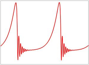
 $\mu$ varies. Obviously, the travelling wave profile exhibits a big principal hump preceded by capillary ripples, which is also called a
 $\gamma _2$-type wave because it has a shape of the solitary hump (Chang et al. Reference Chang, Demekhin and Kopelvitch1993; Liu & Gollub Reference Liu and Gollub1994). However, the interesting fact is that the maximum amplitude as well as the flow rate of the
 $\gamma _2$-type wave profile attenuate with rising values of
 $\mu$, which significantly delays the transition of a viscous fluid from a primary base flow with a flat surface to a nonlinear secondary flow created by the nonlinear wave interactions if the time-reversal symmetry of the viscous fluid is broken. Actually, the increasing amplitude is correlated with the increasing speed of a
 $\gamma _2$-type periodic travelling wave shown in figure 8(a). Hence, the nonlinear interaction between localized periodic travelling waves will be delayed because the speed of the travelling wave reduces as long as
 $\mu$ increases and causes a slower transition to secondary flow. This physical fact can also be understood from the results of the nonlinear spatio-temporal simulation discussed in § 5.3. Moreover, the above result fully supports the stabilizing influence of the odd viscosity coefficient as manifested in the result of primary instability of the base flow. In addition, the local flow rate
 $q$ is non-negative in the capillary regime, and therefore, the backflow phenomenon (Dietze, Leefken & Kneer Reference Dietze, Leefken and Kneer2008) does not seem to occur in the present flow configuration. Figure 9 demonstrates the variation of maximum amplitude
 $h_{max}$ and speed
 $c$ of the solitary wave when the Reynolds number changes. In fact, the solitary waves emerge downstream through a sequence of nonlinear wave interactions, where the fast waves absorb the slow waves in front of them and, ultimately, generate solitary waves with a very large wavelength (Pumir et al. Reference Pumir, Manneville and Pomeau1983; Chang et al. Reference Chang, Demekhin and Kopelvitch1993; Liu & Gollub Reference Liu and Gollub1994; Salamon, Armstrong & Brown Reference Salamon, Armstrong and Brown1994; Chang, Demekhin & Kopelvitch Reference Chang, Demekhin and Kopelvitch1995; Ramaswamy, Chippada & Joo Reference Ramaswamy, Chippada and Joo1996; Vlachogiannis & Bontozoglou Reference Vlachogiannis and Bontozoglou2001; Malamataris, Vlachogiannis & Bontozoglou Reference Malamataris, Vlachogiannis and Bontozoglou2002; Gao, Morley & Dhir Reference Gao, Morley and Dhir2003; Ruyer-Quil & Manneville Reference Ruyer-Quil and Manneville2005; Pradas, Tseluiko & Kalliadasis Reference Pradas, Tseluiko and Kalliadasis2011). It should be noted that the curves in figure 9 exhibit a rapid increase at low Reynolds number followed by a plateau at Reynolds numbers above
 $15$. These two distinct behaviours of amplitude and speed of the solitary wave found in two different regimes of the Reynolds number were identified by Ooshida (Reference Ooshida1999) based on the surface equation for a viscous fluid without an odd viscosity coefficient. In particular, the first one is the drag–gravity regime at low Reynolds number, where the flow dynamics is triggered by viscous drag and gravity, and inertia plays the role of perturbation. On the other hand, the second one is the drag–inertia regime at moderate Reynolds number, where the inertia effect on the flow dynamics is dominant. Figure 10 displays the streamline distribution under the wave in the moving frame for rising values of
 $\mu$, where the recirculation pattern does not appear. As the maximum amplitude of the steady state travelling wave decays as long as
 $\mu$ increases, the surface velocity of the fluid does not exceed the speed of the travelling wave and this fact compensates for the non-existence of recirculation phenomenon under the wave in the moving frame.
(a) Variation of the steady state travelling wave profile for different values of  $\mu$. Solid, dashed and dotted lines stand for
 $\mu =0$,
 $\mu =0.2$ and
 $\mu =0.4$, respectively. The arrow is pointing out the direction of decreasing maximum fluid layer height with increasing
 $\mu$. (b) Variation of the flow rate for the steady state travelling wave for different values of
 $\mu$. Solid, dashed and dotted lines stand for
 $\mu =0$,
 $\mu =0.2$ and
 $\mu =0.4$, respectively. The arrow is pointing out the direction of decreasing maximum flow rate with increasing
 $\mu$. The other flow parameters are
 $k=0.01$,
 $Re=5$,
 $Ca^{-1}=1417$ and
 $\theta =45^{\circ }$.

(a) Variation of the maximum amplitude with Reynolds number for the solitary wave. Solid, dashed and dotted lines stand for  $\mu =0$,
 $\mu =0.2$ and
 $\mu =0.4$, respectively. The arrow is pointing out the direction of decreasing maximum amplitude with increasing
 $\mu$. (b) Variation of the speed with Reynolds number for the solitary wave. Solid, dashed and dotted lines stand for
 $\mu =0$,
 $\mu =0.2$ and
 $\mu =0.4$, respectively. The arrow is pointing out the direction of decreasing speed with increasing
 $\mu$. The other flow parameters are
 $Ca^{-1}=1417$ and
 $\theta =45^{\circ }$.

Streamline distribution in the moving frame: (a)  $\mu =0$, (b)
 $\mu =0.2$, (c)
 $\mu =0.4$. The other flow parameters are
 $k=0.01$,
 $Re=5$,
 $Ca^{-1}=1417$ and
 $\theta =45^{\circ }$.

5.3. Nonlinear spatio-temporal simulation
The nonlinear spatio-temporal evolution of the two-equation model (5.8) and (5.17) is accomplished with the aid of a quasi-linearized Crank–Nicolson scheme (Richtmeyer & Morton Reference Richtmeyer and Morton1967; Kalliadasis et al. Reference Kalliadasis, Ruyer-Quil, Scheid and Velarde2012; Samanta Reference Samanta2014). In fact, the current numerical scheme is consistent with second-order precision in time, while the spatial derivatives are discretized by the central finite difference technique with second-order precision in space. For our own convenience, the two-equation model (5.8) and (5.17) is converted into a matrix form
 \begin{equation} \partial_t\boldsymbol{\mathsf{P}}(x,t)=\boldsymbol{\mathsf{Q}}[\boldsymbol{\mathsf{P}}(x,t)], \end{equation}
where  $\boldsymbol{\mathsf{P}}=(h,q)^T$ is a column matrix while linear and nonlinear terms involving
 $h$,
 $q$ and their spatial derivatives are included in the matrix
 $\boldsymbol{\mathsf{Q}}(\boldsymbol{\mathsf{P}})$. The detailed information on the numerical scheme can be found in Kalliadasis et al. (Reference Kalliadasis, Ruyer-Quil, Scheid and Velarde2012) and Samanta (Reference Samanta2014). In order to perform the numerical simulation, we impose a harmonic periodic forcing at the inlet through the modulation of the flow rate
 \begin{equation} q(0,t)=q_0(1+A \cos 2{\rm \pi} ft), \end{equation}
where  $q_0=2/3$ is the base flow rate at the uniform fluid layer height
 $h_0=1$. Here,
 $f$ is the forcing frequency and
 $A$ is the forcing amplitude. We have imposed a soft boundary condition at the outlet based on the lowest-order hyperbolic wave equation (Samanta, Goyeau & Ruyer-Quil Reference Samanta, Goyeau and Ruyer-Quil2013)
 \begin{equation} \partial_tq + v_f \partial_xq=0, \end{equation}
where  $v_f>0$ is the front velocity. Actually, this outlet boundary condition is used to minimize the generation of upstream propagating disturbances, and enhances the numerical stability. Following the experimental study of Liu & Gollub (Reference Liu and Gollub1994), the spatio-temporal numerical simulation is carried out for a water–glycerin mixture with
 $\rho =10.7 \times 10^{-1}\ \textrm {gm}\ \textrm {cm}^{-3}$,
 $\mu ^{e}=6.7 \times 10^{-2} \ \textrm {gm} \ \textrm {cm}^{-1}\ \textrm {s}^{-1}$,
 $\sigma =6.7 \times 10^1\ \textrm {gm}\ \textrm {s}^{-2}$ and
 $\theta =6.4^{\circ }$ while the viscosity ratio
 $\mu$ changes, or equivalently, the odd viscosity coefficient changes. Figure 11(a) reveals that the small amplitude sinusoidal response evolves spatially into finite amplitude localized waves with a big hump preceded by capillary ripples in the computational domain
 $[0, 2000\ \textrm {mm}]$ when
 $\mu =0$ and
 $f=3\ \textrm {Hz}$, as observed in the experimental work of Liu & Gollub (Reference Liu and Gollub1994). In this case, the primary humps between two localized waves are not well separated from each other because there is a significant overlap between the front and tail of two successive localized waves, which may yield a strong nonlinear interaction among them downstream (see figure 11d). As soon as the effect of the odd viscosity is included, the outcome of the nonlinear response changes drastically. In the presence of
 $\mu$, the small amplitude sinusoidal response undergoes a very slow transition to localized waves with reduced amplitude at
 $\mu =2$ (see figure 11b). If
 $\mu$ is further increased (
 $\mu =4$), the nonlinear response exhibits sinusoidal-type periodic waves in the computational domain
 $[0, 2000\ \textrm {mm}]$ (see figure 11c), where the amplitudes of the sinusoidal-type waves attenuate remarkably by the odd viscosity coefficient. However, if the same numerical experiment is repeated in an extended computational domain
 $[0, 5000\ \textrm {mm}]$, the sinusoidal-type periodic waves appearing in the inception regime turn into saturated multi-peaked waves in the computational domain
 $[4000\ \textrm {mm}, 5000\ \textrm {mm}]$ (see figure 11e). Obviously, localized solitary waves have not formed yet. Next, the numerical simulation is performed when the frequency of the harmonic forcing is
 $f=1.5\ \textrm {Hz}$. The ensuing results can be found in figure 12. Again, a similar scenario happens in the computational domain of interest with increasing
 $\mu$. At
 $\mu =0$, the small amplitude waves immediately turn into a regular train of solitary-type waves with a large teardrop shape followed by capillary ripples after the inception zone (see figure 12a), as found in the experimental work of Liu & Gollub (Reference Liu and Gollub1994). In this case, the solitary-type waves are well separated from each other. Apparently, it seems that the successive solitary-type waves are almost identical to each other (see figure 12d). As soon as
 $\mu$ increases, the transition process from a primary sinusoidal-type wave to a secondary solitary-type wave is delayed significantly in the presence of an odd viscosity coefficient (see figures 12b and 12c). In fact, the solitary-type waves are evolving far away from the inception zone if the numerical experiment is performed in an extended computational domain
 $[0, 5000\ \textrm {mm}]$ (see figure 12e). However, the localized saturated solitary-type waves have not formed yet. From the above results, one can finally conclude that the transition from laminar flow to weak turbulence corresponding to an inlet sinusoidal disturbance will be delayed if the time-reversal symmetry of a viscous fluid is broken.
The spatial evolution of an inlet forcing at large time with frequency  $f=3\ \textrm {Hz}$ when
 $A=0.01$,
 $Re=29$,
 $Ca^{-1}=70$ and
 $\theta =6.4^{\circ }$; (a)
 $\mu =0$, (b)
 $\mu =2$, (c)
 $\mu =4$. (d) A zoomed-in version of panel (a) in the computational domain
 $[1200\ \textrm {mm}, 1600\ \textrm {mm}]$. (e) A zoomed-in version of panel (c) in the computational domain
 $[4000\ \textrm {mm}, 5000\ \textrm {mm}]$.

The spatial evolution of an inlet forcing at large time with frequency  $f=1.5\ \textrm {Hz}$ when
 $A=0.01$,
 $Re=29$,
 $Ca^{-1}=70$ and
 $\theta =6.4^{\circ }$; (a)
 $\mu =0$, (b)
 $\mu =2$, (c)
 $\mu =4$. (d) A zoomed-in version of panel (a) in the computational domain
 $[1200\ \textrm {mm}, 1600\ \textrm {mm}]$. (e) A zoomed-in version of panel (c) in the computational domain
 $[4000\ \textrm {mm}, 5000\ \textrm {mm}]$.

6. Discussion and conclusions
The present manuscript deals with the wave dynamics of a falling viscous fluid with broken time-reversal symmetry. Linear stability analysis is explored based on the Orr–Sommerfeld eigenvalue problem. The long-wave analysis predicts that a surface wave appears in the low Reynolds number regime and the onset of instability for the surface wave is enhanced in the presence of an odd viscosity coefficient. The numerical solution in the arbitrary wavenumber regime shows that the unstable domain induced by the surface mode diminishes as long as the viscosity ratio increases and confirms the stabilizing influence of the viscosity ratio. However, a shear mode appears in the numerical simulation along with the surface mode when the Reynolds number is high and the inclination angle is sufficiently small. It is found that the shear mode can be stabilized by the odd viscosity coefficient. Furthermore, the surface mode controls the primary instability of base flow/parallel flow with a flat surface when the viscosity ratio is low. As soon as the viscosity ratio increases, there exists an unstable range of finite wavenumber where the shear mode controls the primary instability of the base flow rather than the surface mode.
On the other hand, nonlinear stability analysis is explored based on the depth-averaged two-equation model. In the linear regime, the two-equation model recovers the result of the Orr–Sommerfeld eigenvalue problem. In the nonlinear regime, it is found that both the maximum amplitude and flow rate of the steady state travelling wave attenuate as long as the odd viscosity coefficient increases. As a consequence, the fluid surface velocity does not have an opportunity to exceed the speed of the travelling wave to generate a recirculation pattern in the streamline distribution. Since the flow rate in the capillary regime is non-negative, the backflow phenomenon does not seem to occur in the present flow configuration. Finally, the nonlinear spatio-temporal analysis discloses a significant transition delay from primary sinusoidal-type waves to secondary solitary-type waves for a viscous fluid with broken time-reversal symmetry. In fact, this physical fact is responsible for the significant reduction of the amplitude of the travelling wave in the presence of an odd viscosity coefficient. Actually, the increasing amplitude is correlated with the increasing speed of a travelling wave. As a consequence, the nonlinear interaction between evolving travelling waves will be delayed because the speed of the travelling wave reduces as long as  $\mu$ increases and results in a slower transition to the solitary-type wave with a large teardrop shape preceded by capillary ripples.
Acknowledgements
The author would like to thank the anonymous referees for their insightful comments and constructive suggestions on improving the manuscript.
Declaration of interests
The author reports no conflict of interest.



