1. Introduction
A liquid–gas interface (LGI) on surfaces of submerged solid structures is ubiquitous in nature. Since the viscosity of air is approximately 98 % lower than that of water, the LGI has often been regarded as a shear-free surface in theoretical analyses (Philip Reference Philip1972; Crowdy Reference Crowdy2016), leading to the expectation that the LGI could achieve a very large drag reduction (Rothstein Reference Rothstein2010; Huang, Lv & Duan Reference Huang, Lv and Duan2019). Over the last few decades, there has been much research effort aimed at investigating the considerable slip properties of such surfaces (Lee, Choi & Kim Reference Lee, Choi and Kim2016) with the aid of various experimental methods and measurement techniques, such as rheometry (Choi & Kim Reference Choi and Kim2006; Truesdell et al. Reference Truesdell, Mammoli, Vorobieff, van Swol and Brinker2006; Lee, Choi & Kim Reference Lee, Choi and Kim2008), pressure drop measurements (Ou, Perot & Rothstein Reference Ou, Perot and Rothstein2004; Kashaninejad, Nguyen & Chan Reference Kashaninejad, Nguyen and Chan2012) and micro particle image velocimetry (micro-PIV) (Joseph et al. Reference Joseph, Cottin-Bizonne, Benoit, Ybert, Journet, Tabeling and Bocquet2006; Karatay et al. Reference Karatay, Haase, Visser, Sun, Lohse, Tsai and Lammertink2013).
Recently, several micro-PIV experiments of flow over the LGI have reported discrepancies between measured values and theoretical predictions under the shear-free boundary condition (Bolognesi, Cottin-Bizonne & Pirat Reference Bolognesi, Cottin-Bizonne and Pirat2014; Schäffel et al. Reference Schäffel, Koynov, Vollmer, Butt and Schönecker2016; Peaudecerf et al. Reference Peaudecerf, Landel, Goldstein and Luzzatto-Fegiz2017; Song et al. Reference Song, Song, Hu, Du, Du, Choi and Rothstein2018). Peaudecerf et al. (Reference Peaudecerf, Landel, Goldstein and Luzzatto-Fegiz2017) demonstrated that Marangoni stresses induced by traces of surfactant can severely limit the drag reduction of superhydrophobic surfaces. Landel et al. (Reference Landel, Peaudecerf, Temprano-Coleto, Gibou, Goldstein and Luzzatto-Fegiz2019) proposed a theoretical model for the slip and drag of superhydrophobic surfaces with surfactants, which could significantly improve prediction accuracy compared to a surfactant-free model that overestimates the slip length by several orders of magnitude. In this model, the concentration of surfactant is non-uniform in the streamwise direction and it is regarded as uniform in the spanwise direction, which means that only a two-dimensional situation is considered.
Compared with the two-dimensional case, the three-dimensional velocity distribution of flow over arbitrary solid structures with LGIs will be much more complicated. Thus, it is reasonable to presume that a non-uniform concentration distribution of surfactant could be induced in both the streamwise and the spanwise directions for the three-dimensional case. The surfactant-laden flow near the LGI will become more complex and the underlying mechanisms of the effect of surfactants on the three-dimensional flow near the LGI are still not clear. Therefore, a well-designed experiment is required to systematically visualize, quantify and evaluate this effect, which is the scope of the current work.
Surfactants have a significant influence on interfacial flows, such as droplet evaporation (Marin et al. Reference Marin, Karpitschka, Noguera-Marán, Cabrerizo-Válchez, Rossi, Kähler and Valverde2019), bubble flows (Tagawa, Takagi & Matsumoto Reference Tagawa, Takagi and Matsumoto2014), wave breaking and atmosphere–ocean fluxes in the ocean (Tsai & Liu Reference Tsai and Liu2003; Pereira et al. Reference Pereira, Ashton, Sabbaghzadeh, Shutler and Upstill-Goddard2018). A well-known example of the effect of surfactants on the instability of an interfacial flow pattern is the ‘Linde instability’ (Wassmuth, Laidlaw & Coombe Reference Wassmuth, Laidlaw and Coombe1990), which results in switching from a unidirectional flow to a recirculating and oscillating flow. Surfactants are ubiquitous in nature and industry. Even non-cross-linked polydimethylsiloxane (PDMS) chains or impurities could play a role of surfactants and have an effect on the wetting dynamics of soft silicone substrates (Hourlier-Fargette et al. Reference Hourlier-Fargette, Antkowiak, Chateauminois and Neukirch2017). These findings indicate that surfactants can qualitatively alter hydrodynamics.
In this work, a three-dimensional backflow at the LGI is directly observed using micro-PIV. We provide solid evidence that the formation of the backflow is significantly influenced by a surfactant. The origin of the surfactant is the fluorescent particle solution used in micro-PIV, which is often applied to inhibit particle agglomeration and ensure a good dispersibility of particles (Lindken et al. Reference Lindken, Rossi, Große and Westerweel2009; Thermo Scientific 2018). Importantly, we combine experimental measurements, theoretical analyses and numerical simulations to reveal the underlying mechanism of the backflow, which is the surfactant-induced surface tension gradients simultaneously in both streamwise and spanwise directions due to the stagnant lines and the sidewalls confining the LGI. In addition, a kinematic similarity is revealed to govern the backflow under different flow rates. The current work provides a model system for investigating the three-dimensional backflow at the LGI under the influence of surfactants, which is important for underwater applications such as slip boundaries, drag reduction and superhydrophobicity.
2. Theoretical model
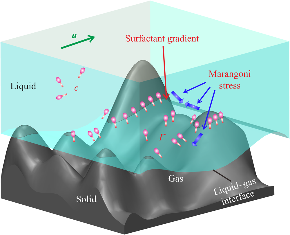
To analyse the effect of surfactants on the flow, a theoretical model for three-dimensional flow over an arbitrary structured solid surface is established with the surfactant adsorbed on the LGI being taken into account (figure 1). The fluid flow is described by the continuity equation and Navier–Stokes equation and the surfactant distribution in the bulk liquid is governed by the convection–diffusion equation:
 \begin{gather} \boldsymbol{\nabla}\boldsymbol{\cdot}\boldsymbol{u}=0, \end{gather}
 \begin{gather} \frac{\partial \boldsymbol{u}}{\partial t}+\boldsymbol{u}\boldsymbol{\cdot} \boldsymbol{\nabla} \boldsymbol{u}=-\frac{1}{\rho}\boldsymbol{\nabla}{p}+\frac{\mu}{\rho}\triangle\boldsymbol{u}, \end{gather}
 \begin{gather} \frac{\partial c}{\partial t}+\boldsymbol{\nabla} \boldsymbol{\cdot}(\boldsymbol{u}c)=D\triangle c, \end{gather}
where  $\boldsymbol {u}=u\boldsymbol {i}+v\boldsymbol {j}+w\boldsymbol {k}$ is the flow velocity,
 $\boldsymbol {i}$,
 $\boldsymbol {j}$,
 $\boldsymbol {k}$ are the direction vectors of Cartesian coordinates,
 $\rho$,
 $p$ and
 $\mu$ are the density, pressure and dynamic viscosity of the liquid, respectively, and
 $c$ and
 $D$ are the bulk concentration and bulk diffusivity of the surfactant, respectively.
Schematic of three-dimensional surfactant-laden flow over the LGI on an arbitrary structure. The geometric constraints of the solid structures induce a non-uniform distribution of the surfactant adsorbed on the LGI, leading to the Marangoni effect in both the streamwise and the spanwise directions, potentially changing the flow pattern near the LGI. Here  $c$ and
 $\Gamma$ are the bulk concentration and interfacial concentration of surfactant, respectively.

On the liquid–solid interfaces, the no-slip boundary condition is written as  $\boldsymbol {u}=0$, and the surfactant cannot diffuse across the interface, which means
 ${\partial c}/{\partial r_n}=0$. On the LGIs, the viscous shear force equals the Marangoni stress (Rosen & Kunjappu Reference Rosen and Kunjappu2012), i.e. (2.4). The transport of surfactant at the interface is governed by the convection–diffusion equation, i.e. (2.5):
 \begin{gather} \mu \frac{\partial \boldsymbol{u}_I}{\partial r_n}= nRT\left(\frac{\Gamma_m}{\Gamma_m-\Gamma}+A\frac{\Gamma}{\Gamma_m}\right){\boldsymbol{\nabla}_I}\Gamma, \end{gather}
 \begin{gather} \frac{\partial \Gamma}{\partial t}+ \boldsymbol{\nabla}_I \boldsymbol{\cdot} (\boldsymbol{u}_I {\Gamma})=D_I{\boldsymbol{\nabla}_I}^2{\Gamma}+S(c_I,{\Gamma}), \end{gather}
where  $\partial (\cdot )/\partial r_n$ indicates the derivative of the inner normal direction, the subscript I denotes the quantities at the interface, n is the surfactant style constant, R is the universal gas constant, T is temperature,
 $\Gamma$ is the interfacial concentration of surfactant,
 $\Gamma _m$ is the maximum interfacial concentration of surfactant, A is the interaction coefficient (Prosser & Franses Reference Prosser and Franses2001) and
 $S(c_I,{\Gamma })$ is the source term. The amount of surfactant due to the process of adsorption and desorption at the interface is denoted by the flux of the surfactant, which is expressed as
 \begin{equation} \left.D \frac{\partial c}{\partial r_n}\right|_I= -S(c_I,{\Gamma}). \end{equation}
The transport of surfactants between bulk and interfaces is coupled using an adsorption–desorption model, i.e. the Frumkin model (Chang & Franses Reference Chang and Franses1995; Fainerman et al. Reference Fainerman, Lylyk, Aksenenko, Liggieri, Makievski, Petkov and Miller2009), in which  $S(c_I,{\Gamma })$ is expressed as
 \begin{equation} S(c_I,{\Gamma})=k_a c_I(\Gamma_m-\Gamma)-k_d\Gamma \,\textrm{e}^{A({\Gamma}/{\Gamma_m})}, \end{equation}
where  $k_a$ and
 $k_d$ represent the adsorption and desorption coefficients, respectively.
When a liquid flows over arbitrary solid structures, three-phase contact lines (TCLs) will form. Since the surfactant adsorbed at the LGI can only flow (transport) along the LGI unless the surfactant diffuses into the bulk through the desorption process, when the fluid near the LGI bypasses the obstacles, the surfactant at the LGI will be blocked near the TCLs rather than moving with the bulk flow, leading to the accumulation of the surfactant near the TCLs and thus a non-uniform distribution of surfactant at the LGI. According to (2.4), an interfacial concentration gradient of surfactant will generate Marangoni stresses at the LGI, which are likely to influence the original flow pattern in the case where the Marangoni effect is strong enough to resist the shear force. This is the typical scenario at the microscale where the surface tension dominates. In §§ 3 and 4, we describe well-designed experiments based on the above theoretical analyses to investigate the effect of surfactants on the three-dimensional flow near the LGI.
3. Experimental methodology
3.1. Experimental set-up
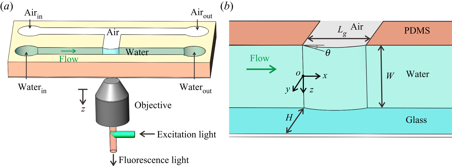
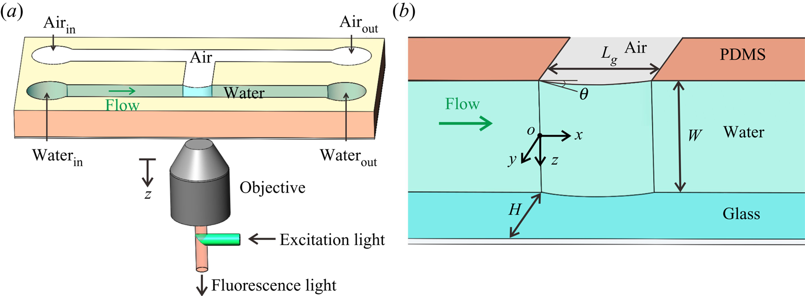
To investigate the effect of surfactants contained in particle solutions on the three-dimensional flow field near the LGI in micro-PIV measurements, a microfluidic device consisting of two main parallel microchannels was designed (figure 2 $a$), in which one microchannel was intended for liquid and the other was intended for gas. A side channel was fabricated to connect the two main channels, and the LGI was formed at the joining point of the main and side channels. The TCLs around the LGI allow the development of the surfactant concentration gradient in both streamwise and spanwise directions as discussed in § 2. The microchannels were made of PDMS obtained using demoulding technology (Tsai et al. Reference Tsai, Peters, Pirat, Wessling, Lammertink and Lohse2009). A coverslip with a thickness of 170
 ${\rm \mu }$m was treated with oxygen plasma and then bonded to the microchannels through van der Waals adhesion.
Schematic of the experimental set-up. (a) Three-dimensional view of the microchannel with a confined LGI. (b) Geometry in the region of the LGI in detail. The length and width of the LGI are  $L_g=100 {\rm \mu }$m and
 $W=100 {\rm \mu }$m, respectively, and the width of the microchannel is
 $H=100 {\rm \mu }$m. The origin of coordinates is located at the midpoint of the upstream stagnation line.
The geometry of the LGI is determined by the pressure difference between the gas and the liquid phases (Lv et al. Reference Lv, Xiang, Xue, Lin and Duan2017). The gas pressure was regulated to maintain the protruding angle of the meniscus  $\theta =25^{\circ }$ under different flow rates (Karatay et al. Reference Karatay, Haase, Visser, Sun, Lohse, Tsai and Lammertink2013). An inverted microscope (IX73, Olympus, Japan) was employed to observe and measure the geometry of the LGI as well as the flow field. The LGI was stable and symmetric during the experiments, as both the Weber number (
 $We$) and the capillary number (
 $Ca$) are sufficiently small. In the experiments,
 $We=(\rho U^2 L_g)/\sigma$ ranges from
 $3\times 10^{-6}$ to
 $2\times 10^{-3}$ and
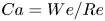 $Ca=We/Re$ ranges from
 $2\times 10^{-5}$ to
 $5\times 10^{-4}$ as the mean velocity of the inlet liquid flow U ranges from 1.39 to 34.75 mm s
 $^{-1}$, and consequently the Reynolds number
 $Re=(\rho UH)/\mu$ varies from 0.319 to 34.75, where
 $\sigma$ is the surface tension of water. The flow rate of liquid was regulated by an infusion syringe pump (Pump 11 Elite, Harvard Apparatus, USA) with a volume flow uncertainty of 0.5 %, which indicates that the flow in our experiments can be regarded as uniform.
3.2. Micro-PIV measurement
A typical micro-PIV implementation was conducted to quantify the flow field over the LGI. The tracer particle solution consisted of degassed ultrapure water (Dura 12, The Lab, USA) seeded with fluorescent polystyrene particles (Thermo Fisher Scientific, Fluro-Max, Red Fluorescent Polystyrene Microspheres 542/612, 1  ${\rm \mu }$m in diameter) in a volume ratio of 4 : 1. The peak excitation wavelength of the fluorescent particles is 542 nm (green light) and the peak emission wavelength is 612 nm (red light). To characterize the subsequent behaviour of the fluorescent particles in the flow, we calculated the Stokes number (St) and the ratio of Stokes number to Froude number (Fr) (Mathai et al. Reference Mathai, Calzavarini, Brons, Sun and Lohse2016). The Stokes number is expressed as
 $St\equiv t_0 U_{\textit{max}} / r_c$, where
 $t_0\equiv (\rho _p d_{p}^2/18\mu )(1+\rho /(2\rho _p))$ is the characteristic time,
 $U_{\textit{max}}$ (
 $=3.128$ mm s
 $^{-1}$) is the maximum fluid velocity,
 $r_{c}$ (
 $=100 {\rm \mu }$m) is the characteristic length of the microchannel,
 $d_{p}$ (
 $=1 {\rm \mu }$m) is the diameter of tracer particles,
 $\rho _p$ (
 $=1.05$ g cm
 $^{-3}$) and
 $\rho$ (
 $=0.998$ g cm
 $^{-3}$) are the densities of the tracer particles and water, respectively, and
 $\mu$ (
 $= 10^{-3}$ Pa s) is the dynamic viscosity of water. The factor
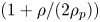 $(1+\rho /(2\rho _p))$ accounts for the added mass force (Oliveira, Van der Geld & Kuerten Reference Oliveira, Van der Geld and Kuerten2015). The buoyancy-corrected Froude number is defined as
 $Fr\equiv U_{\textit{max}}^2/ (r_cg(1-\rho /\rho _p))$, where g is the gravitational acceleration. The calculated value of
 $St$ (equivalently the ratio of particle response time to the characteristic time scale in the flow) is
 $10^{-6}$, which indicates an acceptable flow tracing accuracy (Samimy & Lele Reference Samimy and Lele1991). The calculated value of
 $St/Fr$ (equivalently the ratio of particle drift velocity to Kolmogorov velocity) is
 $10^{-2}$, which indicates an acceptable deviation from ideal tracer behaviour induced by gravity (Diddens et al. Reference Diddens, Tan, Lv, Versluis, Kuerten, Zhang and Lohse2017).
A continuous laser (power of 5 W) at 532 nm (LWGL532-5W, Laserwave, China) was used for channel illumination. Image pairs were captured at different  $z$ planes of the microchannel using a high-speed camera (Phantom V2512, USA) with a resolution of
 $512\ \textrm {pixel} \times 384\ \textrm {pixel} \times 8$ bit at a rate of 4000–10 000 frames per second for various flow rates. An objective (UPLFLN
 $20\times$,
 $\textrm {NA} = 0.5$,
 $\textrm {WD} = 2.1$ mm) was used to observe the particle motion. The configuration of the micro-PIV enables visualization of the profile of the LGI. By regulating the position of the focal plane of the objective, the flow field in the various horizontal planes perpendicular to the
 $z$ direction was visualized and measured.
A single-pixel correlation method was used for the micro-PIV images with higher particle concentrations, which can significantly improve the spatial resolution of the near-wall flow field (Westerweel, Geelhoed & Lindken Reference Westerweel, Geelhoed and Lindken2004; Kähler, Scholz & Ortmanns Reference Kähler, Scholz and Ortmanns2006; Kähler, Scharnowski & Cierpka Reference Kähler, Scharnowski and Cierpka2012; Zhu et al. Reference Zhu, Yuan, Zhang and Lee2013). The interrogation view of the micro-PIV images was  $512\ \textrm {pixel} \times 384\ \textrm {pixel}$ (
 $365\ {\rm \mu } \textrm {m} \times 274\ {\rm \mu }\textrm {m}$). The images were analysed with a customized MATLAB program for 4096 image pairs. When processing the data, the sample window size was only a single pixel (
 ${\sim }0.7 {\rm \mu }$m). For each measurement, bright-field images were acquired to determine the protruding angle and to define the locations of the meniscus and walls on the raw micro-PIV images. The measurement uncertainty is shown in appendix C.
The hybrid PIV–particle tracking velocimetry (PTV) method was applied to evaluate the micro-PIV images with lower particle concentrations. The evaluation starts with a standard PIV algorithm to predict the vectors. The PIV computations were processed starting with  $64\ \textrm {pixel} \times 64\ \textrm {pixel}$ interrogation windows and decreasing to
 $16\ \textrm {pixel} \times 16\ \textrm {pixel}$. The resolution of the vector field was then further refined by detecting and tracking individual particles by the PTV algorithm, which increases the number of vectors per PIV interrogation window from one to the total number of particles per same window. The particle detection method adapted in DaVis 10.0.5 (Lavision, Germany) looks for the position of the highest intensity and arranges an interrogation window of the size of the particle diameter around the position of the maximum intensity. The PTV interrogation window in the second frame is shifted by the predicted vector from the PIV calculations. Finally, an individual particle correlation will correlate the intensity pattern of both windows to determine the exact shift. The same post-processing median filter applied to the PIV results was also applied to the PTV results. A final step of converting the vector field to a
 $16\ \textrm {pixel} \times 16\ \textrm {pixel}$ grid was then applied using a second-order polynomial fit (Stanislas et al. Reference Stanislas, Okamoto, Kähler and Westerweel2005; Alharbi & Sick Reference Alharbi and Sick2010).
3.3. Determination of surfactant type and concentration
In order to determine the type of surfactant in the commercial fluorescent particle solutions (sample) used in micro-PIV experiments, Fourier transform ion cyclotron resonance mass spectrometry (FTICR-MS) was performed, as detailed in appendix A. The experiments were completed at the Analytical Instrumentation Center of Peking University. The mass spectrum of the sample was obtained using a FTICR-MS instrument (Solarix XR, Bruker, Germany), which demonstrated that the type of surfactant is Triton X-100 by comparing the mass spectrum of the sample with that of Triton X-100 in Brinded, Tiller & Lane (Reference Brinded, Tiller and Lane1993) and Dong et al. (Reference Dong, Chen, Corti, Franses, Zhao, Ng and Hanson2011).
In addition, to determine the bulk concentration of the surfactant (Triton X-100) in the sample, 10  ${\rm \mu }$l of commercial Triton X-100 (Sigma Chemical Co.) was diluted with ultrapure water (Dura 12, The Lab, USA) at a volume ratio of 1 : 20 000. Likewise, 10
 ${\rm \mu }$l of fluorescent polystyrene particle solution (Thermo Fisher Scientific, USA) was diluted with ultrapure water at a volume ratio of 1 : 4, which was the same as that in the micro-PIV experiments, and the solution was centrifuged for the supernatant. Then,
 $10^{-6}$ mol l
 $^{-1}$ angiotensin II (human) was added into the two diluted solutions as an internal standard, followed by FTICR-MS experiments to obtain the corresponding mass spectra. By analysing the mass spectra of the diluted Triton X-100 and the diluted sample with corresponding internal standards, the bulk concentration of surfactant (Triton X-100) can be determined to be
 $c_0=0.04$ mol m
 $^{-3}$.
3.4. Three-dimensional numerical simulation
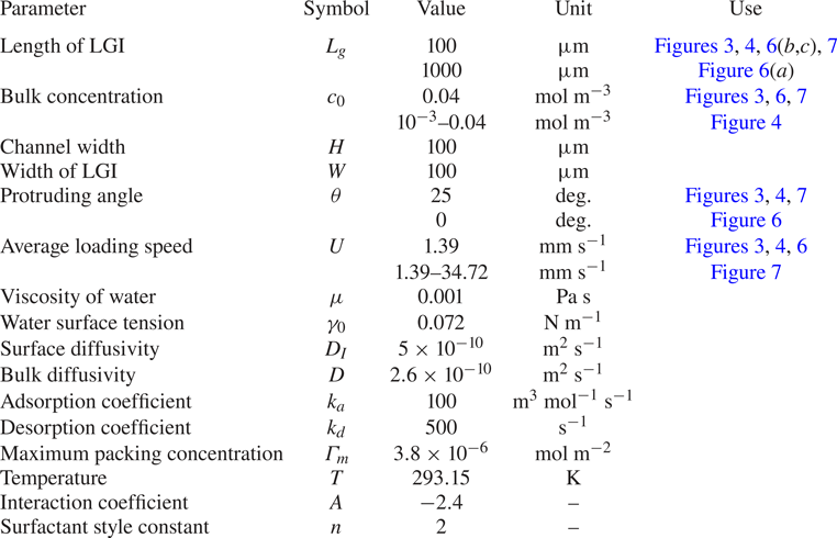
Three-dimensional numerical simulations were performed to study the effect of the surfactant on the flow near the LGI using COMSOL Multiphysics. The type of element are P1-P1 Lagrange elements and 8-node hexahedron. To ensure mesh independence, four sets of meshes were compared before conducting the formal calculations, as detailed in appendix B. To implement the model, in COMSOL Multiphysics, we combine the laminar flow module with a dilute species transport module for the transport equations in the bulk ((2.1)–(2.3)). The equation for the transportation of surfactant on the LGI is implemented through (2.5) with a source term corresponding to the kinetic flux  $S$. This flux also serves to implement the boundary condition (2.6) at the LGI for the dilute species transport module. The governing equations (2.1)–(2.7) were simultaneously solved using the parameters in table 4, with
 $\hat{\boldsymbol{u}}_0 (\hat{y},\hat{z})={4\hat{y}}(1-\hat{y})(1-{4\,\hat{z}^{\,2}}/{\widehat W^2})$ employed as the inlet condition and the weak form of (2.5) added to the shear-free boundary condition on the LGI to capture the Marangoni effect. A pressure-driven flow with the same geometric parameters in the experiments was solved. The no-slip boundary condition was applied to the liquid–solid interfaces. The parameters used in the simulations were determined according to the literature on Triton X-100 and the adsorption dynamics of surfactant at the air–water interface. Specifically, the main parameters of surfactant, such as surface diffusivity and bulk diffusivity, were taken from Eckmann & Cavanagh (Reference Eckmann and Cavanagh2003). The adsorption and desorption coefficients of surfactant were taken from Peaudecerf et al. (Reference Peaudecerf, Landel, Goldstein and Luzzatto-Fegiz2017). Maximum packing concentration of surfactant was achieved by fitting the experimental results, with magnitude kept identical to that in Lin, McKeigue & Maldarelli (Reference Lin, McKeigue and Maldarelli2003) and Chang & Franses (Reference Chang and Franses1995). Specific parameters used in the simulations of the surfactant-laden flow and other simulation details are provided in table 4.
4. Results and discussion
4.1. Backflow phenomenon
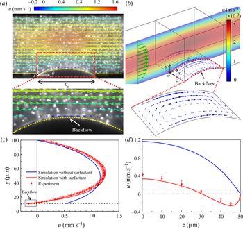
Figure 3(a) shows the flow field experimentally measured above the LGI in the plane of  $z=40 {\rm \mu }$m. An unexpected flow moving opposite to the mainstream is visualized at the LGI, which is referred to as backflow. The influence of gravity on the geometry of the LGI and the flow field can be neglected as the Bond number
 $Bo=(\rho g r^2)/\sigma \approx 10^{-3}\ll 1$, where
 $r=118 {\rm \mu }$m is the meniscus radius (Yu et al. Reference Yu, Lu, Lohse and Zhang2015; Diddens et al. Reference Diddens, Tan, Lv, Versluis, Kuerten, Zhang and Lohse2017). Therefore, only half of the microchannel was measured due to the symmetry of flow. Backflow can be observed from
 $z=32$ to
 $z= 50 {\rm \mu }$m (see supplementary movie 1 available at https://doi.org/10.1017/jfm.2020.426), while no backflow occurs from
 $z=0$ to
 $z=32 {\rm \mu }$m (see supplementary movie 2). Figure 3(
 $b$) shows the numerical simulation result of the flow field for surfactant-laden flow, clearly illustrating two vortices that develop over the entire LGI and evolve symmetrically with respect to the centreline of the meniscus along the mainstream, which numerically verifies the formation of backflow.
Backflow phenomenon at the LGI. (a) Velocity field of surfactant-laden flow measured by micro-PIV superimposed on a raw micro-PIV image. The geometry of the LGI is denoted by the dashed lines with a protruding angle  $\theta =25^{\circ }$. The flow rate
 $Q= 0.05$ ml h
 $^{-1}$. (b) Numerical results of the surfactant-laden flow, using the same parameters as for the experiments. The coloured contours indicate the flow velocity in the intermediate cross-section of the microchannel. The green and blue arrows denote the velocities in the bulk and at the LGI, respectively. (c) The local velocity profile above the vertex of the LGI (i.e. the white filled point in a). The horizontal dashed line denotes the position of the vertex. (d) The slip velocities along the vertex line of the LGI, showing a reduced slip performance due to the presence of surfactant.
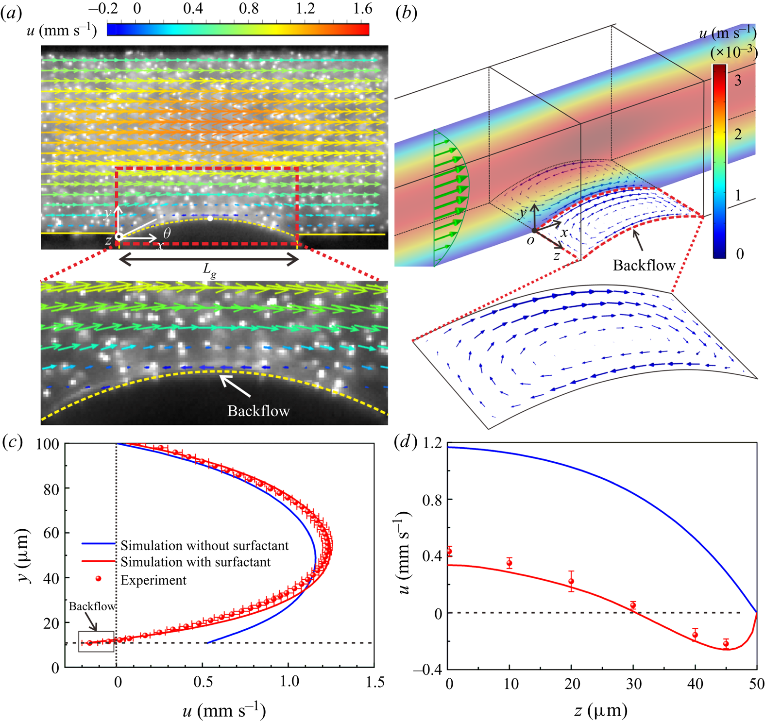
The local velocity profile above the vertex of the LGI (i.e.  $x=L_g/2$) in the plane of
 $z=40 {\rm \mu }$m is experimentally quantified, as shown in figure 3(
 $c$). A negative slip velocity at the LGI indicates flow opposite to the direction of the mainstream, namely backflow. The numerical predictions in figure 3(
 $c$) show that, for surfactant-free flows, only forward velocity was obtained rather than backflow or vortices. The numerical velocity profile of the surfactant-laden flow presents a significant difference from that of the surfactant-free flow, which quantitatively exhibits the effect of surfactants on the three-dimensional flow field near the LGI from the perspective of numerical predictions. Further, we conducted experiments to examine the effect of surfactant on the flow field, which will be addressed in detail below, as presented in § 4.2.1 and appendix A. Figure 3(
 $d$) shows the slip velocities along the vertex line of the meniscus, which reflects a degradation of the slip performance over the entire LGI due to the presence of surfactant.
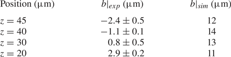
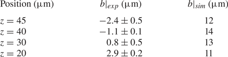
The quantitative impact of the surfactant can be evaluated by measuring local slip lengths. According to Navier's slip boundary condition,  $u|_{interface}=b(x) (\partial u/\partial y)|_{interface}$ (Schönecker, Baier & Hardt Reference Schönecker, Baier and Hardt2014; Schäffel et al. Reference Schäffel, Koynov, Vollmer, Butt and Schönecker2016),
 $b(x)$ is the local slip length, which varies for different locations on the LGI. The local velocity profiles above the vertex of the meniscus on different
 $xy$ planes were obtained from the micro-PIV measurements of the surfactant-laden flow and the numerical simulations of the surfactant-free flow, which are used to calculate the local slip lengths.
The quantities of the local slip lengths listed in table 1 clearly show that the surfactant-laden flow substantially reduces the slip performance of the LGI, which is consistent with observations in previous literature (Bolognesi et al. Reference Bolognesi, Cottin-Bizonne and Pirat2014; Schäffel et al. Reference Schäffel, Koynov, Vollmer, Butt and Schönecker2016; Peaudecerf et al. Reference Peaudecerf, Landel, Goldstein and Luzzatto-Fegiz2017; Song et al. Reference Song, Song, Hu, Du, Du, Choi and Rothstein2018). Negative local slip lengths are obtained at  $z=40$ and
 $z=45 {\rm \mu }$m in the experiments, demonstrating that the surfactant not only weakens the flow near the LGI, but also reverses the local flow, reflecting the discrepancy between the measured values and the theoretical expectations.
Local slip length on the LGI.
4.2. Mechanism of formation of backflow
According to the actual conditions in the experiments, the basic governing equations (2.1)–(2.7) can be simplified and non-dimensionalized as follows. A flat LGI is employed in this section for the convenience of theoretical analyses. As  $Re$ is small, the flow is regarded as steady and the mass conservation equation (2.1) and Navier–Stokes equation (2.2) can be written as
 \begin{equation} \widehat{\boldsymbol{\nabla}} \boldsymbol{\cdot}\hat{\boldsymbol{u}}=0, \quad \widehat{\boldsymbol{\nabla}}\xi =\widehat{\triangle} \hat{\boldsymbol{u}}, \end{equation}
where  $\hat {\boldsymbol {u}}={\boldsymbol {u}}/{U}$ and
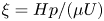 $\xi ={H}{p}/({\mu U})$. Considering that the surface adsorption of surfactant has little effect on the bulk liquid, the bulk concentration
 $c$ can be regarded as a constant
 $c_0$. Therefore, the convection–diffusion equation (2.3) can be disregarded.
For boundary conditions, on the liquid–solid surfaces at  $\hat{y}= 1$ and
 $\hat{z}=\pm \widehat W/2 (\widehat W=W/H )$, we have
 $\hat {\boldsymbol {u}}=0$. On the LGI at
 $\hat{y}= 0$,
 $0<\hat{x}< \widehat {L}_g$ (
 $\widehat L_g=L_g/H$), we have
 $\hat{v}=0$, where
 $\hat{x}=x/H$,
 $\hat{y}=y/H$,
 $\hat{z}=z/H$. In addition, as the interfacial Peclet numbers
 $Pe_I=L_g U/D_I \sim 10^{2}\gg 1$, the effect of the surface diffusion can be ignored. Equations (2.4) and (2.5) are approximated as
 \begin{equation} \frac{\partial \hat{\boldsymbol{u}}_I}{\partial \hat{y}}= \widehat{\boldsymbol{\nabla}}_I \eta, \quad \Phi{\widehat{\boldsymbol{\nabla}}_I}\boldsymbol{\cdot} \hat{\boldsymbol{u}}_I= -\eta, \end{equation}
where  $\eta ={nRT\Gamma _1}/({\mu U})$ and
 $\Phi =nRT\Gamma _0/[\mu H (k_a c_0 +k_d)]$. We define
 $\Gamma _0=k_a c_0\Gamma _m/ (k_a c_0+k_d,\textrm {e}^{A\Gamma _0/\Gamma _m}$) as the interfacial concentration of surfactant when the process of adsorption and desorption at the interface is balanced in the stationary fluid and
 $\Gamma _1=\Gamma -\Gamma _0$.
The solution to equations (4.1) and (4.2),  $\hat {\boldsymbol {u}}(\hat{x},\hat{y},\hat{z})$,
 $\xi (\hat{x},\hat{y},\hat{z})$ and
 $\eta (\hat{x},\hat{y},\hat{z})$, depends only on three dependent parameters
 $\Phi$,
 $\widehat L_g$ and
 $\widehat W$, referring to the presence of the surfactant and the geometric features of the microchannel related to the length and width of the LGI. Therefore, it is reasonable to conclude that the formation of backflow is significantly influenced by the three parameters.
4.2.1 Effect of bulk concentration of surfactant
To evaluate the effect of the bulk concentration of surfactant ( $c_0$, non-dimensionalized as
 $\Phi =nRT\Gamma _0/[\mu H (k_a c_0 +k_d)]$, where
 $\Gamma _0=k_a c_0\Gamma _m/(k_a c_0+k_d\,\textrm {e}^{A\Gamma _0/\Gamma _m}$)) on the backflow,
 $|U_b |_{\textit{max}}$, the maximum velocity of backflow at the vertex line of the LGI, and
 $W_b$, the width of the backflow region, i.e. the distance between the sidewall and the location where the fluid velocity is zero, are employed to determine the intensity and the structure of the backflow, respectively. We define
 $|\widehat {U}_b |_{\textit{max}}=|{U}_b|_{\textit{max}}/U$ as the dimensionless maximum velocity of backflow and
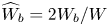 $\widehat {W}_b=2W_b/W$ as the dimensionless width of the backflow region. An amount of 100
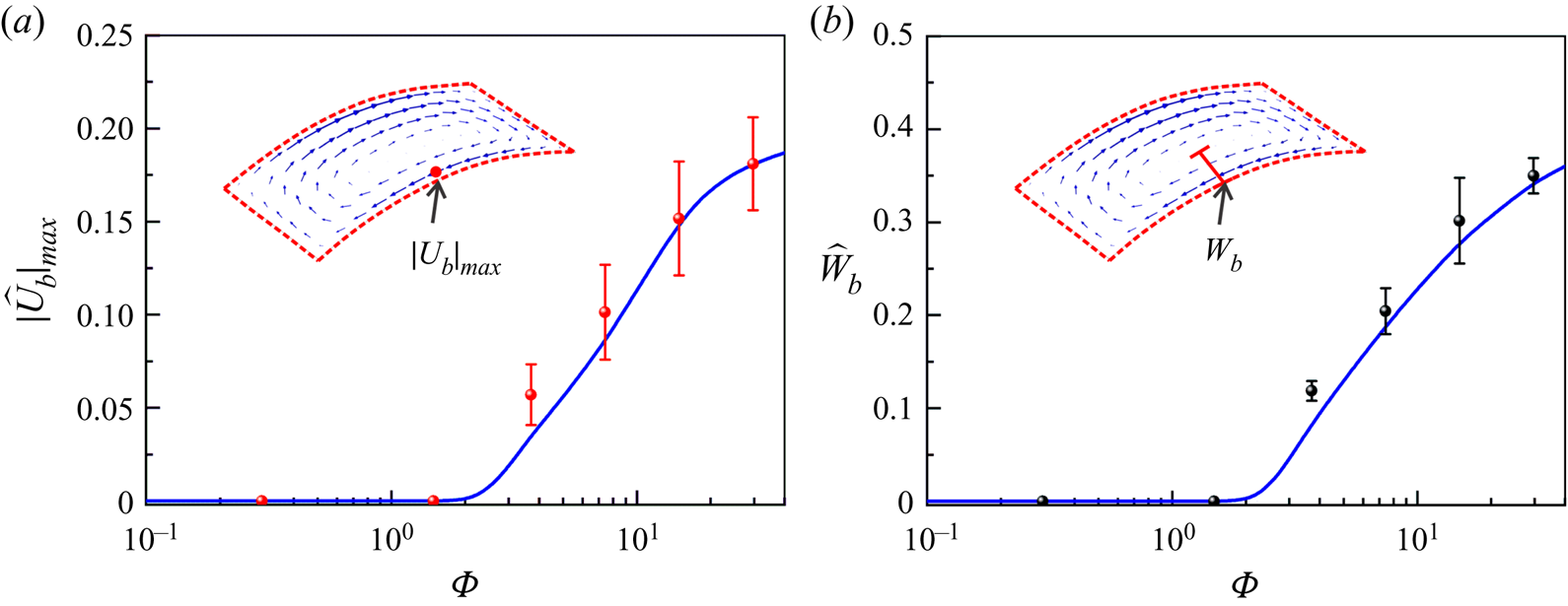
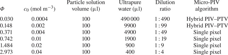
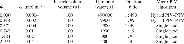
 ${\rm \mu }$l of fluorescent polystyrene particle solution (Thermo Fisher Scientific, USA) was diluted with ultrapure water at various volume ratios to obtain micro-PIV particle solutions with different bulk concentrations of surfactant, as shown in table 2. Figures 4(a) and 4(
 $b$) show the variations of
 $|\widehat {U}_b|_{\textit{max}}$ and
 $\widehat {W}_b$ as a function of
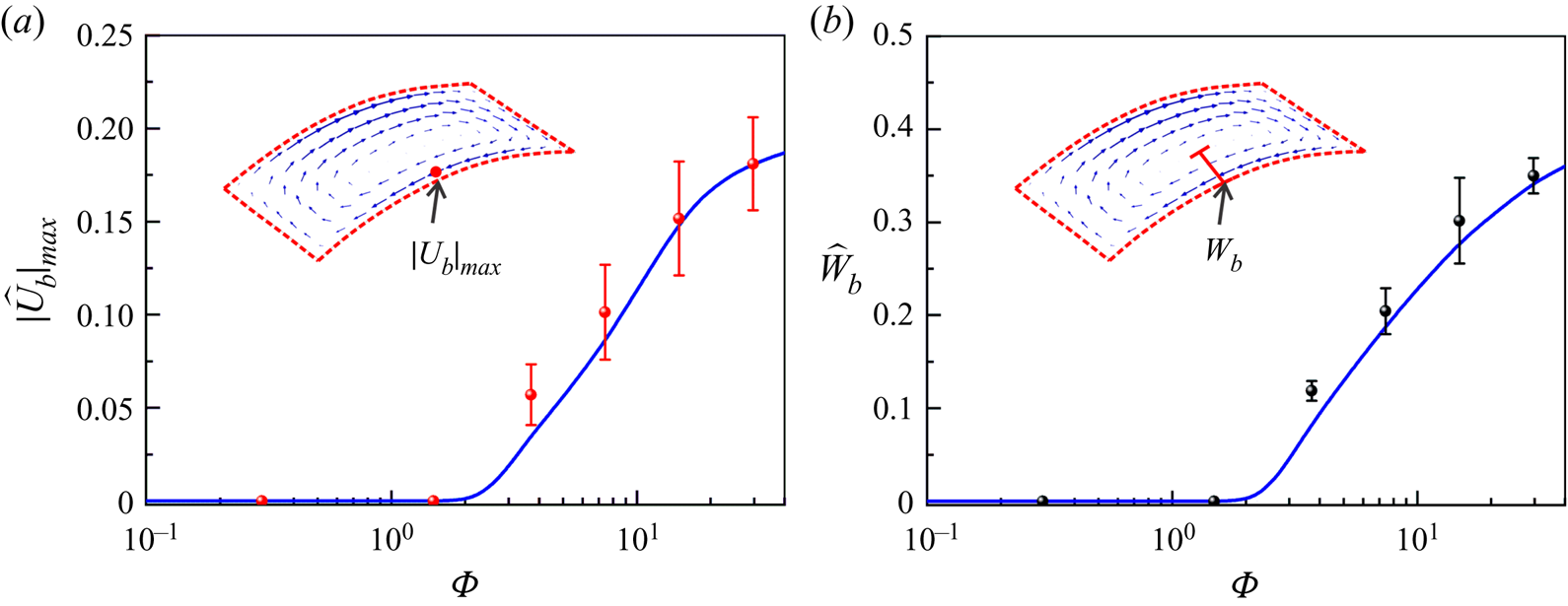
 $\Phi$, respectively. On the one hand, when
 $\Phi <0.2$, corresponding to
 $c_0 < 0.003$ mol m
 $^{-3}$, no backflow is obtained as
 $|\widehat {U}_b |_{\textit{max}}\approx 0$ as well as
 $\widehat {W}_b\approx 0$. On the other hand, when
 $\Phi >0.2$, corresponding to
 $c_0 >0.003$ mol m
 $^{-3}$, the larger the bulk surfactant concentration, the stronger is the backflow, indicated by the increase of both
 $|\widehat {U}_b|_{\textit{max}}$ and
 $\widehat {W}_b$ as
 $\Phi$ increases. The experimental results and numerical simulation results are in good agreement, as shown in figure 4. Therefore, we can draw two conclusions. (1) When the bulk concentration is low, the backflow will vanish, which clearly demonstrates that the surfactant has a significant effect on the formation of the backflow. (2) The bulk concentration of the surfactant is crucial to the determination of the intensity and the structure of the backflow.
(a) Effect of the dimensionless bulk concentration of surfactant  $\Phi$ (
 $\Phi =nRT \Gamma _0/[\mu H (k_a c_0 +k_d)]$, where
 $\Gamma _0=k_a c_0\Gamma _m/(k_a c_0+k_d\,\textrm {e}^{A\Gamma _0/\Gamma _m}$)) on the dimensionless maximum backflow velocity
 $|\widehat{U}_b |_{\textit{max}}$. (b) Effect of the dimensionless bulk concentration of surfactant
 $\Phi$ on the dimensionless width of the backflow region
 $\widehat {W}_b$.
Preparation of micro-PIV particle solutions with various bulk concentrations of surfactant.
4.2.2 Effect of the geometric features of the LGI
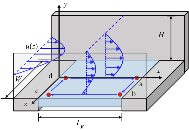
As the presence of the surfactant has been verified to be a determinant for the formation of backflow, we focus here on the effect of the geometric features of the LGI on the formation of backflow. First, we theoretically analyse the effect of the downstream stagnation line (i.e. line ab in figure 5) on the streamwise concentration distribution of surfactant at the LGI. A two-dimensional situation (as shown in the  $xy$ plane in figure 5) is considered to analyse the streamwise concentration distribution of surfactant at the LGI. Surfactants are advected by the flow and accumulate at the downstream stagnation line, which consequently leads to a streamwise interfacial concentration gradient
 $\partial \eta /\partial \hat{x}$. When the flow reaches a steady state, the Marangoni stress induced by the surfactant concentration gradient is balanced by the viscous force near the LGI,
 ${(\partial \hat{u}}/{\partial \hat{y})}|_I= {\partial {\eta }}/{\partial \hat{x}}$. For simplicity, a linear velocity gradient is assumed, i.e.
 $(\partial \hat{\boldsymbol{u}}/\partial \widehat {y})|_I = \alpha (\widehat U_{H/2}-\hat{u}_I)$, where
 $\widehat U_{H/2}$ is the velocity at half the width of the microchannel,
 $\hat{u}_I$ is the velocity at the LGI and
 $\alpha$ is a prefactor greater than zero. Thus, in the streamwise direction, the distribution of
 $\eta$ is
 \begin{equation} \eta (x)=\alpha \widehat U_{H/2} \left(\hat{x}-\frac{\widehat{L}_g}{2}\right)+C. \end{equation}
As  $\eta$ is odd symmetric about
 $\hat{x}=\widehat {L}_g/2$, we have
 $\eta =0$ at line
 $\hat{x}=\widehat {L}_g/2$, which indicates
 $C=0$.
Mechanism of formation of backflow on the LGI. Four characteristic points a, b, c and d are selected for analysing the distribution of the interfacial concentration.
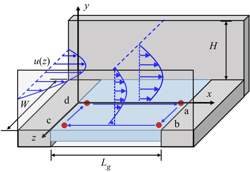
Second, due to the influence of the sidewall, the flow is non-uniform in the spanwise direction, resulting in non-uniform spanwise concentration distribution of the surfactant. The inlet flow is regarded as a square tube flow, and the velocity distribution can be approximated as the product of two quadratic Poiseuille flows in the y and z directions,  $\hat{\boldsymbol{u}}_0 (\hat{y},\hat{z})={4\hat{y}}(1-\hat{y})(1-{4\hat{z}^2}/{\widehat W^2})$. Therefore, if we do not consider the flow or diffusion in the
 $z$ direction, the flow regime should be similar to that of the two-dimensional flow field for each horizontal position (
 $xy$ plane). Combining the velocity distribution in the middle of the microchannel
 $\widehat U_{H/2}=(1-4\hat{z}^2/{\widehat W^2})$ and (4.3), we have
 \begin{equation} \eta(x,z)={\alpha}\left(\hat{x}-\frac{\widehat{L}_g}{2}\right)\left(1-\frac{4\hat{z}^2}{\widehat W^2}\right). \end{equation}
Taking the four points a, b, c and d in figure 5 as characteristic points, the interfacial concentration relationships are  $\eta (\textrm {a})>\eta (\textrm {b})$ and
 $\eta (\textrm {c})> \eta (\textrm {d})$ based on (4.4). As both points b and c are very close to the sidewall,
 $\eta (\textrm {b})\approx \eta (\textrm {c})\approx 0$.
The interfacial concentration gradient in the spanwise direction results in Marangoni flow, which indicates that (4.4) is not the equilibrium state. Therefore, the equilibrium concentration distribution ( $\eta ^{\ast }$) should take into account the corrections caused by spanwise Marangoni flow which directs the advection of surfactant from point a to point b as well as from point c to point d. As a result, the interfacial concentration relationship of these four characteristic points is
 $\eta ^{\ast }(\textrm {a})>\eta ^{\ast }(\textrm {b}) > \eta ^{\ast }(\textrm {c})> \eta ^{\ast }(\textrm {d})$ in the equilibrium state. According to (4.2a) and considering
 $\widehat U_{H/2}=0$ at
 $\hat{z} = \pm \widehat W/2$, we have
 \begin{equation} \hat{u}_I^\ast|_{bc}=-\left.\frac{\partial \eta^\ast}{\partial \hat{x}}\right|_{bc}< 0. \end{equation}
Thus, the negative value of velocity near the sidewall (i.e.  $u_I^\ast |_{bc}$) corresponds to the backflow observed in our experiments and three-dimensional simulation for surfactant-laden flow. Therefore, the mechanism of formation of backflow is theoretically revealed to be a consequence of the competition between the mainstream and the Marangoni flow generated by the concentration gradient of surfactant over the LGI, where the geometric features of the microchannel substantially affect the concentration distribution of the surfactant.
In order to verify the influence of two geometric features on the formation of backflow, increases of  $\widehat L_g$ and
 $\widehat W$ are implemented in COMSOL Multiphysics. First, the LGI is lengthened to
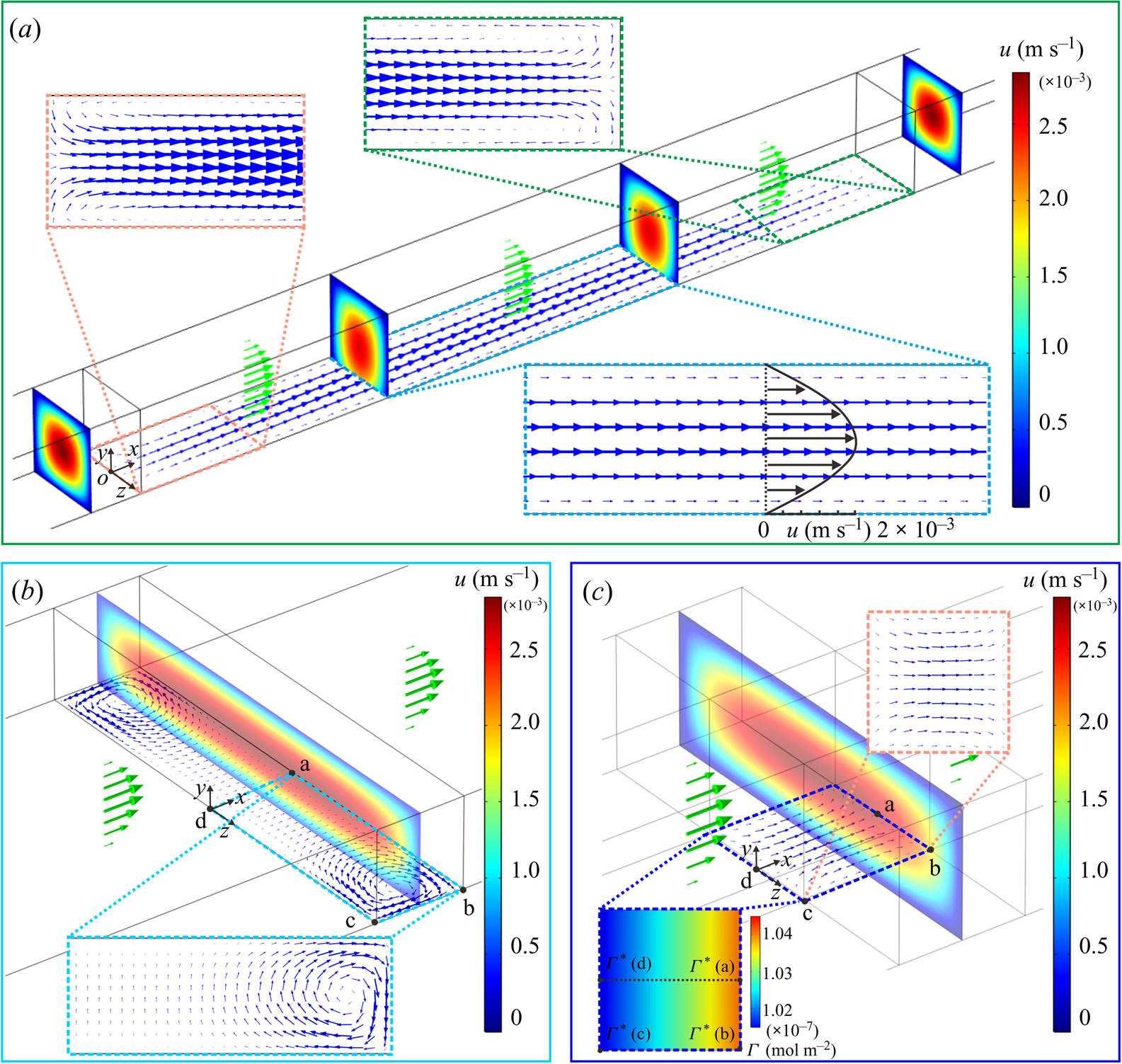
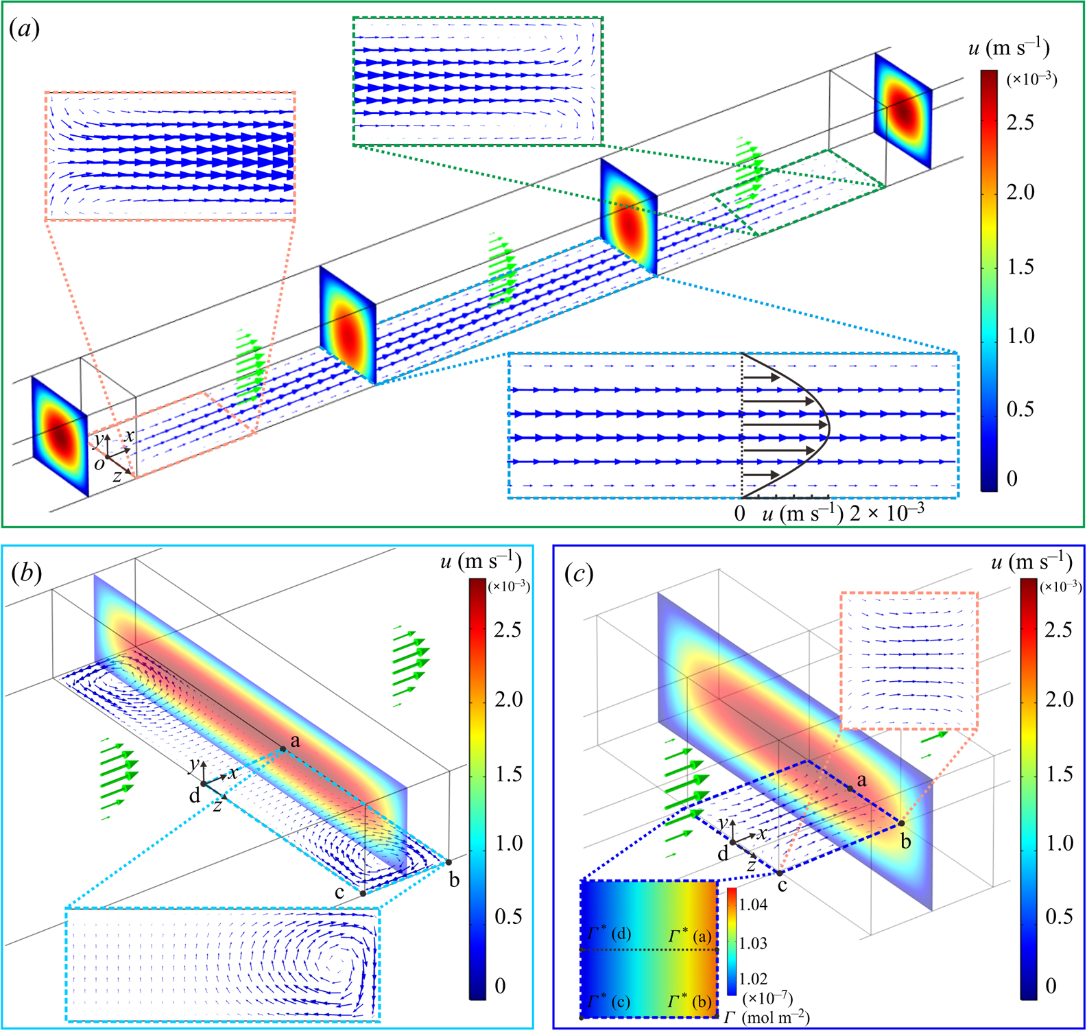
 $L_g=1$ mm along the streamwise direction to increase the distance between the upstream and downstream stagnation lines, which will reduce the streamwise surfactant gradient over the LGI (Peaudecerf et al. Reference Peaudecerf, Landel, Goldstein and Luzzatto-Fegiz2017). The simulation results demonstrate that backflow no longer occurs at the centre part of the long meniscus due to the significant decrease of the concentration gradient in the streamwise direction, as shown in the magnified plot of the velocity at the LGI in figure 6(a). Although the streamwise concentration gradient decreases, backflow still occurs at the corners formed by the stagnation lines and the sidewalls, as shown in the magnified plot of the velocity at the side parts of the long meniscus in figure 6(a). Second, the LGI is widened to
 $W=500\,{\rm \mu }$m along the spanwise direction to increase the distance between the sidewalls, which will reduce the spanwise surfactant gradient over the plastron. The simulation results demonstrate that although the spanwise concentration gradient decreases, backflow still occurs near the sidewalls, as shown in the magnified plot of the velocity at the LGI in figure 6(
 $b$). Therefore, we can conclude that as long as both the stagnation lines in the streamwise direction and the confining sidewalls in the spanwise direction exist, three-dimensional backflow will always occur.
(a) The case of extending the length of the LGI to  $L_g=1$ mm. The magnified plot shows the velocity field at the side parts of the LGI; the backflow still occurs at the corners formed by the stagnation lines and the sidewalls. (
 $b$) The case of extending the width of the LGI to
 $W=500 {\rm \mu }$m. The magnified plot shows the velocity field at the meniscus; the backflow still occurs at the corners formed by the stagnation lines and the sidewalls. (
 $c$) The case of releasing the spanwise confinement of the LGI. The magnified plots show both the interfacial concentration and the velocity field on the LGI. The magnified plot on the left-hand side shows that the spanwise concentration gradients along lines ab and cd vanish as the confinement is released. In (
 $a$–
 $c$), the average loading speed
 $U=1.39$ mm s
 $^{-1}$ and the other parameters in the microfluidic system are unchanged except the geometric features of the LGI. The coloured contours indicate the flow velocity in the intermediate cross-section of the microchannel. The green arrows indicate the bulk velocities and the blue arrows indicate the interfacial velocities.
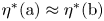
If one wants to eliminate the backflow at the LGI, either the streamwise concentration gradients or the spanwise concentration gradients, or even both of them, need to be zero to eliminate the three-dimensional distribution of Marangoni flow at the LGI. The two extreme cases correspond to the releases of the stagnation lines and the confining sidewalls. For the first case, in order to eliminate the streamwise concentration gradient (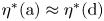 $\eta ^{\ast }(\textrm {a})\approx \eta ^{\ast }(\textrm {d})$ and
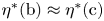 $\eta ^{\ast }(\textrm {b})\approx \eta ^{\ast }(\textrm {c})$) the distance between the upstream and downstream stagnation lines should be infinitely long, which can be realized in annular flows (Lee et al. Reference Lee, Choi and Kim2008; Song et al. Reference Song, Song, Hu, Du, Du, Choi and Rothstein2018). For the second case, in order to eliminate the spanwise concentration gradient (
 $\eta ^{\ast }(\textrm {a})\approx \eta ^{\ast }(\textrm {b})$ and
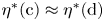 $\eta ^{\ast }(\textrm {c})\approx \eta ^{\ast }(\textrm {d})$), which corresponds to making the confining sidewalls disappear at the LGI, this can be realized in a circular pipe whose surface contains periodically distributed regions of LGI, similar to that used by Lauga & Stone (Reference Lauga and Stone2003). As an approximation for the second case, the spanwise confinement of the LGI, i.e. the sidewalls, is released, as shown in figure 6(
 $c$). The depth of the microchannel is increased from 100 to 300
 ${\rm \mu }$m, while the width of the microchannel and the length and width of the LGI,
 $H=100 {\rm \mu }$m,
 $L_g=100 {\rm \mu }$m and
 $W=100 {\rm \mu }$m, remain unchanged. The position of the LGI is still in the centre of the microchannel. The simulation results clearly illustrate that the Marangoni effect in the spanwise direction cannot be achieved to drive spanwise flow as almost no gradient of surfactant concentration is generated, which inhibits the formation of backflow as shown in figure 6(
 $c$). Overall, the mechanism of formation of backflow is revealed to be a competition between the mainstream and the Marangoni flows generated by the interfacial concentration gradients of surfactant in both streamwise and spanwise directions.
It is worth noting that, for rectangular longitudinal superhydrophobic gratings without sidewall confinement, e.g. the cases in Bolognesi et al. (Reference Bolognesi, Cottin-Bizonne and Pirat2014) and Peaudecerf et al. (Reference Peaudecerf, Landel, Goldstein and Luzzatto-Fegiz2017), backflow does not occur because the interfacial concentration of surfactant in the spanwise direction is approximately uniform, which is similar to the situation in figure 6(c) that reflects a two-dimensional problem.
4.3. Characteristics of backflow
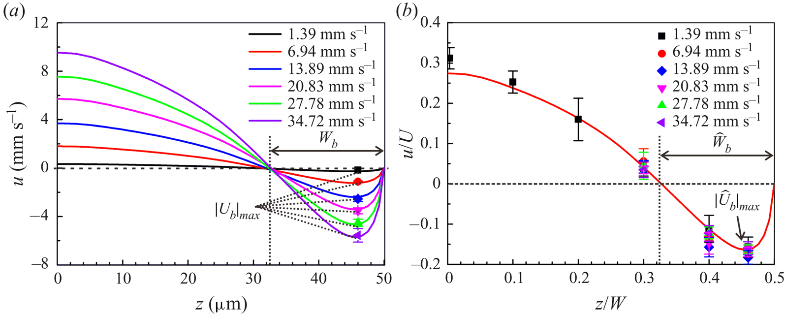
Figure 7(a) shows the numerical velocity distribution at the vertex line of the LGI with protruding angle  $\theta =25^{\circ }$ and surfactant concentration
 $c_0 =0.04$ mol m
 $^{-3}$ under various flow rates. As the average loading speed
 $U$ increases,
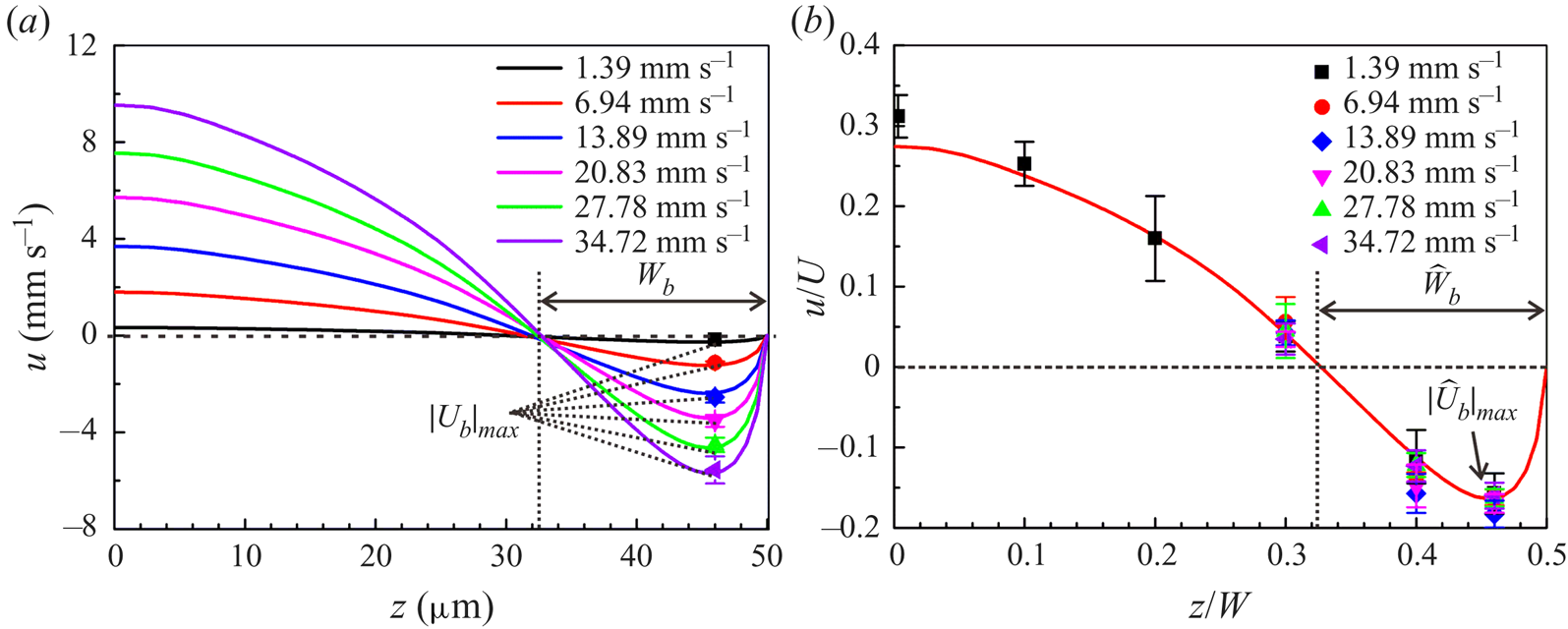
 $|{U}_b|_{\textit{max}}$ increases concurrently, which indicates that a high mainstream flow rate strengthens the intensity of the backflow. The experimental data exhibit good agreement with the numerical predictions of the maximum backflow velocity. However, the maximum backflow velocities occur at a fixed location, and the width of the backflow region remains unchanged in figure 7(a). These two invariances reflect a similar backflow structure, which suggests the kinematic similarity of the backflow. This kinematic similarity can be revealed through the features of
 $\Phi$,
 $\widehat L_g$ and
 $\widehat W$, which are irrelevant to the mainstream flow rate. According to the theoretical analysis in § 4.2, when
 $\Phi$,
 $\widehat L_g$ and
 $\widehat W$ remain unchanged, the dimensionless flow field
 $\hat {\boldsymbol {u}}(\hat{x},\hat{y},\hat{z})$ will be unchanged, indicating the kinematic similarity of the backflow. Figure 7(
 $b$) plots the experimental results and the numerical dimensionless velocity distribution at the vertex line of the LGI obtained. This agreement reveals the kinematic similarity which governs the characteristics of backflow and can be used to predict the backflow behaviour.
Characteristics of backflow. (a) The velocity distribution at the vertex line of the LGI with protruding angle  $\theta =25^{\circ }$ under various flow rates. The bulk concentration of surfactant
 $c_0=0.04$ mol m
 $^{-3}$. The solid lines represent the numerical velocity profiles. The filled symbols represent the experimental maximum backflow velocities. Different colours represent different average loading speeds
 $U$. (
 $b$) Dimensionless velocity distribution at the vertex line of the LGI, showing the kinematic similarity of the backflow. The solid line represents the numerical dimensionless velocity distribution. The filled symbols represent the experimental dimensionless velocities, collapsing well onto the numerical curve. Here
 $|\widehat {U}_b |_{\textit{max}}=|{U}_b|_{\textit{max}}/U$,
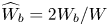 $\widehat {W}_b=2W_b/W$.
5. Conclusion
In conclusion, three-dimensional backflow is directly visualized, which is demonstrated to be significantly influenced by surfactant and generated by the interfacial concentration gradients of surfactant in both streamwise and spanwise directions. A kinematic similarity governing the characteristics of backflow is obtained, which can be used to predict the backflow behaviour under different flow rates. Based on the mechanism of the formation of backflow, strategies such as reducing the bulk concentration of surfactant and releasing the stagnation lines or the confining sidewalls can be applied to eliminate the backflow. The backflow mechanism may also prove useful for designing microfluidic devices aiming to enhance the transport of fluids and particles. The current work provides physical insights into the effect of surfactant on the three-dimensional backflow, which is important for studies of the LGI, such as slip boundaries, drag reduction and superhydrophobicity. This is especially concerning for marine applications, e.g. ship drag reduction with LGI, as it is well documented that seawater contains significant amounts of surfactants.
Acknowledgments
This work was supported by the National Natural Science foundation of China (NSFC) under grants nos. 11988102, 91848201, 11521202, 11872004 and 11802004 and Young Elite Scientists Sponsorship Program by China Association for Science and Technology (CAST) under grant 2017QNRC001. The authors thank H. Yuan for help with micro-PIV data processing. The determination of surfactant type and concentration in commercial fluorescent particle solutions was finished at the Analytical Instrumentation Center of Peking University by W. Zhou.
Declaration of interests
The authors report no conflict of interest.
Supplementary movies
Supplementary movies are available at https://doi.org/10.1017/jfm.2020.426.
Appendix A. Determination of surfactant type and concentration
The fluorescent polystyrene particles (Thermo Fisher Scientific, Fluro-Max, Red Fluorescent Polystyrene Microspheres 542/612, 1  ${\rm \mu }$m in diameter) used in micro-PIV measurement were purchased from Sigma-Aldrich (St Louis, MO, USA). To determine the type of surfactant in commercial fluorescent polystyrene particle solutions (sample), we firstly took the supernatant from a 10
 ${\rm \mu }$l centrifuged sample, and then mixed it with the matrix solution DHB (20 mg ml
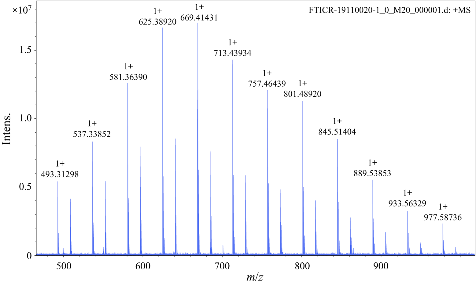
 $^{-1}$ in 60 % acetonitrile) (Sigma-Aldrich) in a volume ratio of 1 : 1. The mass spectrum of the sample was obtained using FTICR-MS (Solarix XR, Bruker, Germany), as shown in figure 8. The mass-to-charge ratio (
 $m/z$) is shown on the horizontal axis and the intensity of the signal on the vertical axis.
Mass spectrum of fluorescent polystyrene particle solution (sample).
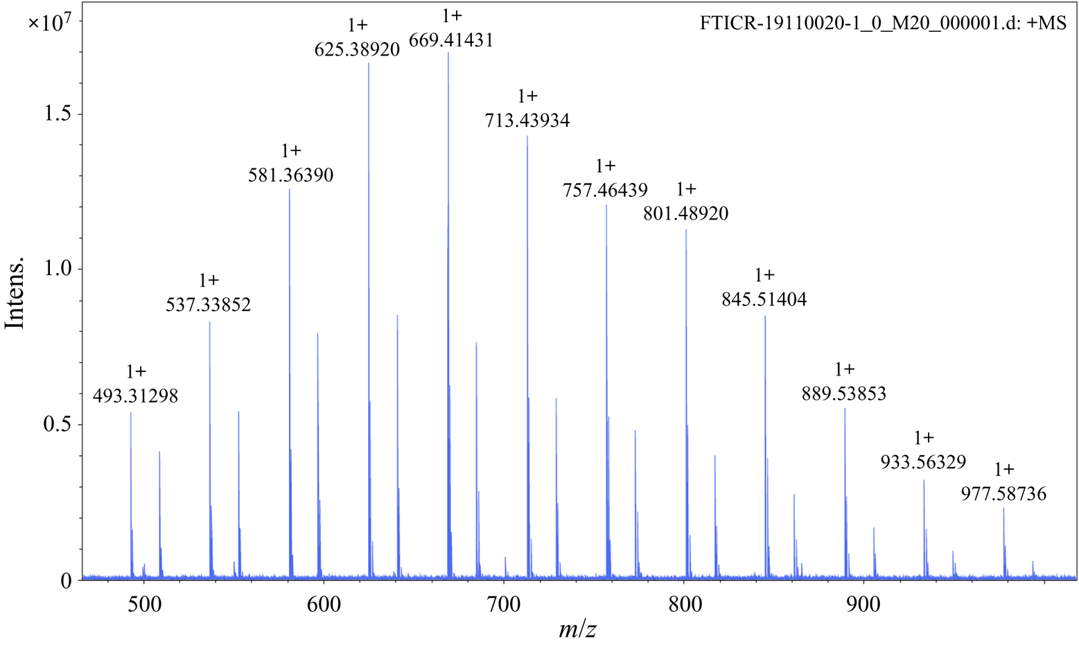
Through a search of the literature, we found that the mass spectrum of the fluorescent polystyrene particle solution is the same as that of Triton X-100 (see figure 1 in Brinded et al. (Reference Brinded, Tiller and Lane1993) and figure S1 in Dong et al. (Reference Dong, Chen, Corti, Franses, Zhao, Ng and Hanson2011)).
Note that the observed peaks in our sample are sodium (Na $^+$) adducts and those observed by Brinded et al. (Reference Brinded, Tiller and Lane1993) are ammonium (NH
 $_4^+$) adducts. For example,
 $m/z = 576$ in Brinded et al. (Reference Brinded, Tiller and Lane1993) and Dong et al. (Reference Dong, Chen, Corti, Franses, Zhao, Ng and Hanson2011) corresponds to
 $m/z= 581$ in our mass spectrum since the molecular weight of NH
 $_4^+$ is 5 smaller than that of Na
 $^+$, indicating the consistency between the mass spectra of the particle solution and the commercial Triton X-100. Therefore, the type of surfactant in the commercial fluorescent polystyrene particle solution is strongly consistent with being Triton X-100.
Next, we determined the concentration surfactant (Triton X-100) in commercial fluorescent polystyrene particle solutions (sample). Firstly, we took 10  ${\rm \mu }$l Triton X-100 (Sigma Chemical Co.) with ultrapure water (Dura 12, The Lab, USA) at a volume ratio of 1 : 20 000 and added
 $10^{-6}$ mol l
 $^{-1}$ angiotensin II (human) as an internal standard to obtain Mixture 1. Secondly, we took a 10
 ${\rm \mu }$l sample of fluorescent polystyrene particle solution (Thermo Fisher Scientific, USA) with ultrapure water at a volume ratio of 1 : 4, which is the same as that in the micro-PIV experiments, and centrifuged the solution for the supernatant. Similarly, we added
 $10^{-6}$ mol l
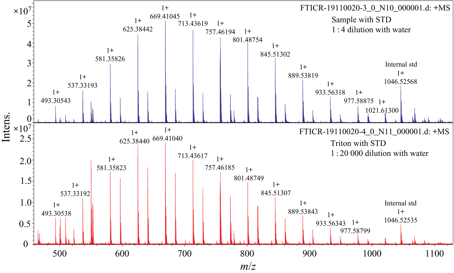
 $^{-1}$ angiotensin II (human) as an internal standard into the supernatant to obtain Mixture 2. The mass spectra of these two mixtures were collected using FTICR-MS as shown in figure 9. As the concentration of Triton X-100 is known, the concentration of particle solution sample (analyte) can be determined by monitoring the analyte-to-internal standard ratio, which corresponds to the ion signal ratio of analyte to internal standard (Pirman et al. Reference Pirman, Kiss, Heeren and Yost2012).
Comparison of the mass spectra of diluted Triton X-100 and diluted sample with corresponding internal standards.
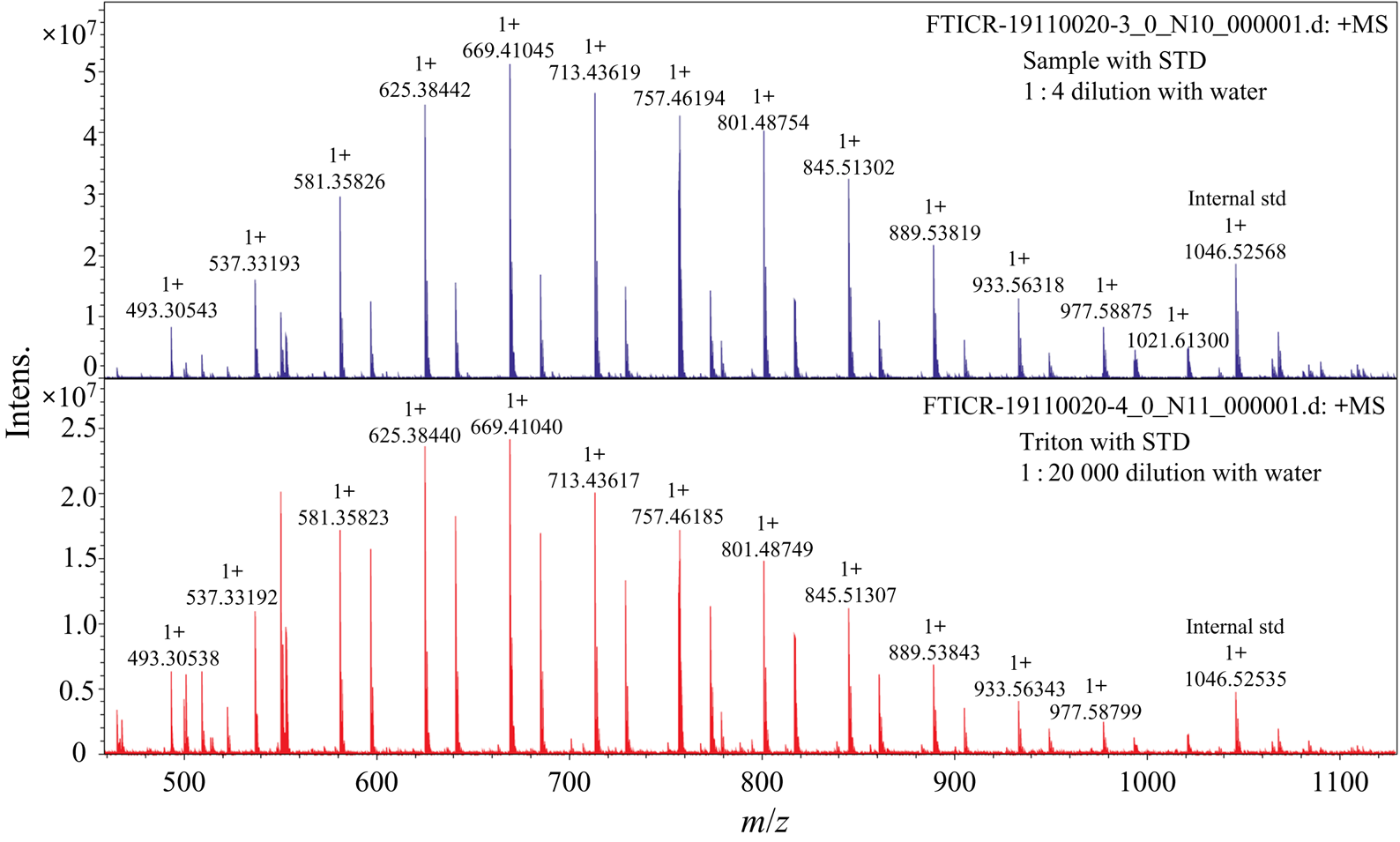
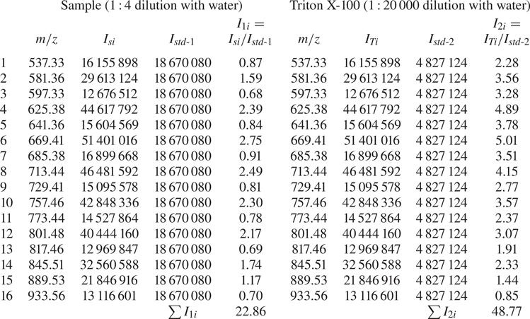
According to the mass spectra shown in figure 9, we took each component with signal intensity higher than 20 % of the highest peak for analysis, as shown in table 3. The  $m/z$ values, each component signal intensity and corresponding internal standards of the sample and Triton X-100 are shown in table 3. The signal intensity of each component in the diluted sample solution is represented by
 $I_{1i}$ and that of the corresponding internal standard is represented by
 $I_{std\text {-}1}$. The signal intensity of each component in the diluted Triton X-100 is represented by
 $I_{2i}$ and that of the corresponding internal standard is represented by
 $I_{std\text {-}2}$. The concentration of each component of the diluted Triton X-100 solution,
 $C_{Ti}$, is given by
 \begin{equation} C_{Ti}={C_T}{I_{2i}}\left/\,\sum{I_{2i}}\right., \end{equation}
where  $C_T=\rho _T/(20\,000M_T)=0.086$ mol m
 $^{-3}$ is the concentration of diluted Triton X-100 solution,
 $\rho _T$ is the density of Triton X-100 (
 $\rho _T=1.07 \times 10^{6}$ g m
 $^{-3}$) and
 $M_T$ is the average molecular weight (
 $M_T=625$ g mol
 $^{-1}$).
Determination of the concentration of surfactant (Triton X-100).
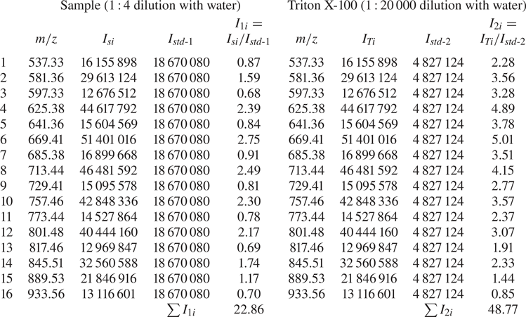
The concentration of each component of the diluted sample solution,  $C_{Si}$, is given by
 \begin{equation} C_{Si}={C_{Ti}}{I_{1i}}/{I_{2i}}={C_{T}}{I_{1i}}\sum{I_{2i}}. \end{equation}
Therefore, the total concentration of the diluted sample solution is
 \begin{equation} C_{S}=\sum{C_{Si}}={C_{T}}\sum{I_{1i}}\left/\,\sum{I_{2i}}\right.=0.04\ \text{mol m}^{-3}. \end{equation}
Besides, the mass-to-charge ratios of the sample and Triton X-100 in figure 9 are in a good agreement with each other, which suggests once again that the surfactant contained in the micro-PIV particle solutions is strongly consistent with being Triton X-100.
Appendix B. Three-dimensional surfactant-laden simulations
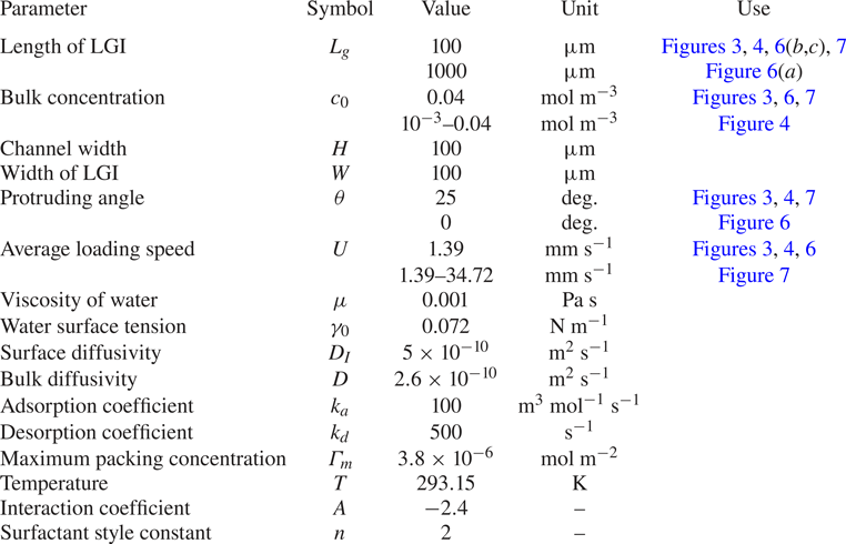
Specific parameters used in the simulations of the surfactant-laden flow and other simulation details are provided in table 4.
Parameters for the simulations of three-dimensional surfactant-laden flow.
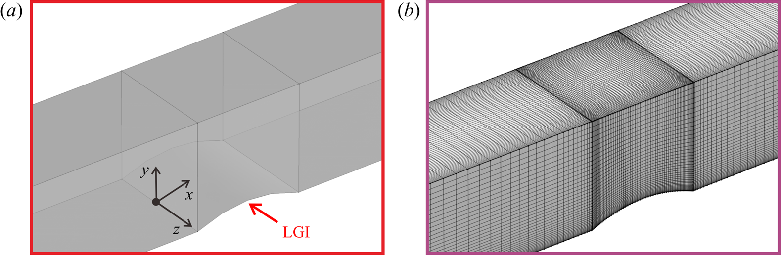
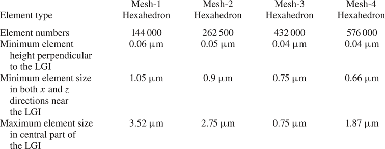
In order to ensure mesh independence, four sets of meshes were compared before conducting the formal calculations. The mesh is gradually encrypted from mesh-1 to mesh-4. Detailed information is listed in table 5. The simulating domain is shown in figure 10( $a$) and the mesh (mesh-3, for example) is shown in figure 10(
 $b$).
The simulating domain ( $a$) and mesh-3 (
 $b$).

Detailed information about the meshes.
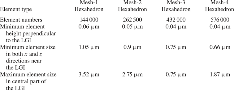
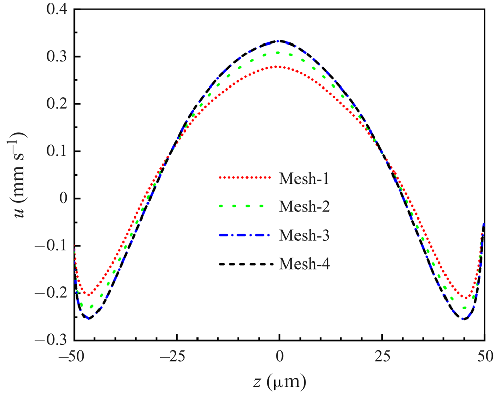
Figure 11 presents the four velocity profiles along the vertex line of the LGI calculated based on four sets of meshes, which clearly shows that the velocity profile based on mesh-3 is in agreement with denser mesh-4. Therefore, mesh independence is verified and mesh-3 is chosen as the computational mesh for parameter studies in the current work.
Comparing the velocity profiles along the vertex line of the LGI for the four sets of meshes.

Appendix C. Measurement uncertainty evaluation
We investigated the systematic errors and the uncertainty of the single-pixel algorithm based on the synthetic PIV images. The details are as follows.
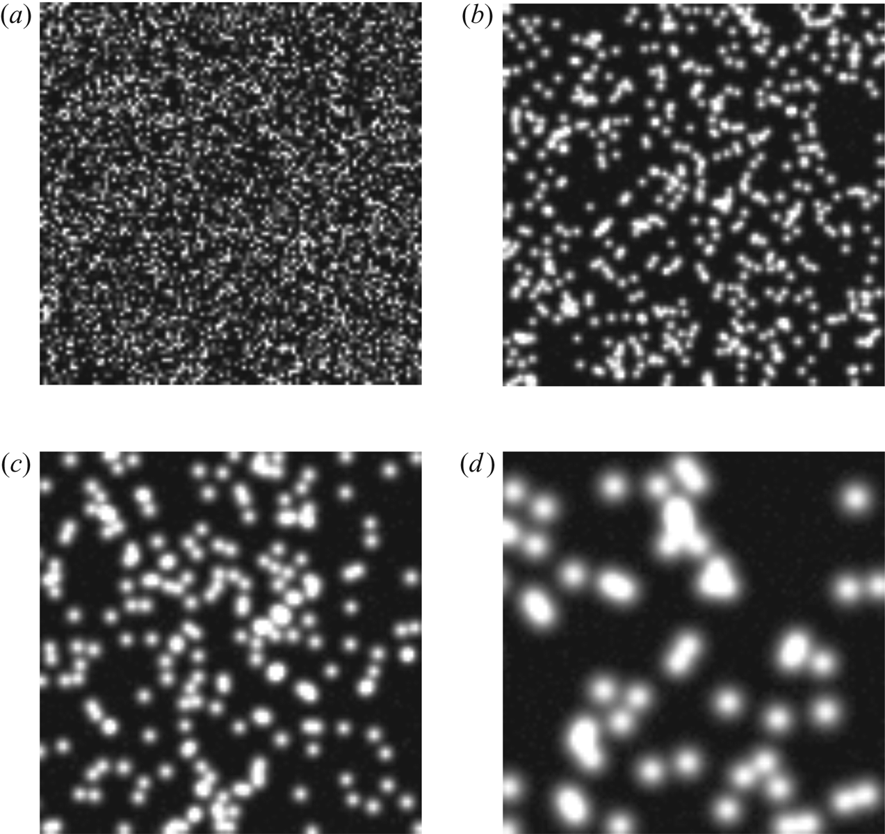
First, we analysed the bias errors of the single-pixel algorithm for velocity near the wall based on the synthetic PIV images. The synthetic PIV images have different digital particle image diameters  $D$. The centre positions of the particle images were randomly distributed to simulate uniform seeding concentrations (Kähler et al. Reference Kähler, Scharnowski and Cierpka2012). The intensity for an individual pixel was computed from the integral of a Gaussian function (where
 $D$ is four times the standard deviation) over the pixel's area, representing a sensor fill factor of one. In addition, we also added Gaussian noise with an average intensity of zero and a standard deviation of 1 % of the maximum intensity of the particle images to simulate a 100 : 1 signal-to-noise ratio. The digital particle image diameter varied from
 $D = 1$ to 10 pixel, which is typical for experiments, as illustrated in figure 12. Ten thousand image pairs were generated for each
 $D$. The particle concentration is approximately 40 %, which means that 40 % of the image is covered by particles. A velocity profile with a constant velocity gradient of
 $\partial {\rm \Delta} X^*/\partial Y^*=0.1$ was simulated to illustrate the sensitivities. Here
 $Y^*$ is the position away from the wall and
 ${\rm \Delta} X^*$ is the wall-parallel displacement.
(a–d) Synthetic PIV images with digital particle image diameter  $D=1$, 3, 5 and 10 pixel, respectively.

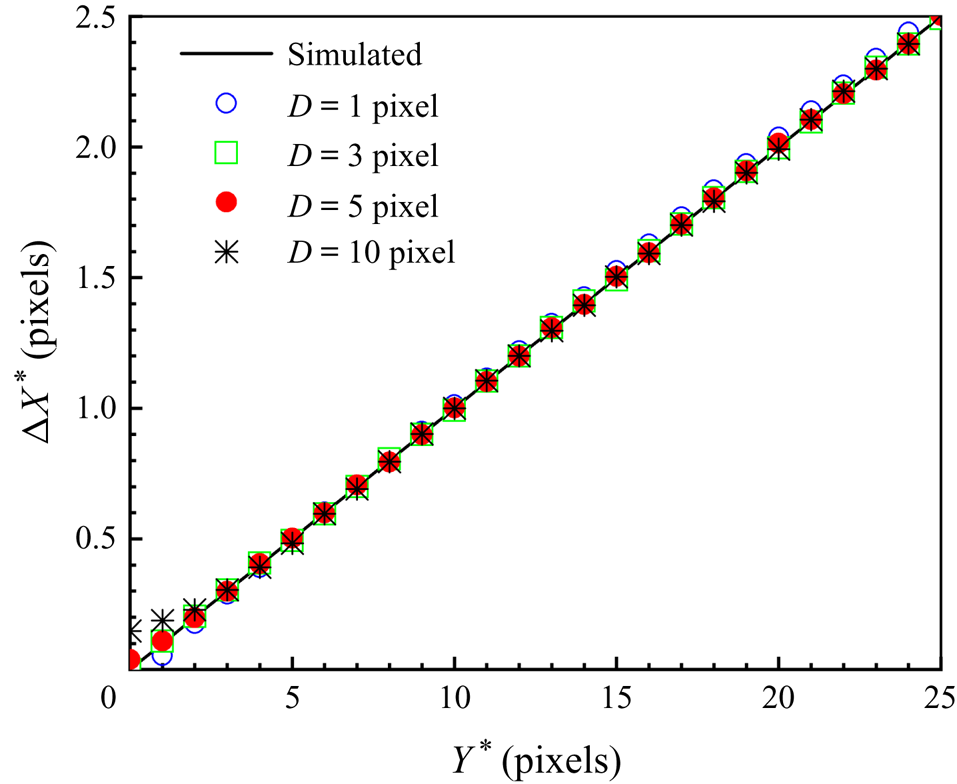
Figure 13 shows the estimated wall-parallel displacement profiles for a simulated constant velocity gradient ( $\partial {\rm \Delta} X^*/\partial Y^*=0.1$) in the near-wall region using the single-pixel algorithm for different
 $D$. The systematic error can be expressed by
 $\delta {\rm \Delta} X^*=|{\rm \Delta} X^*_{estimated}(Y^*)-{\rm \Delta} X^*_{true}(Y^*)|$ (Kähler et al. Reference Kähler, Scharnowski and Cierpka2012). For
 $D = 1$ pixel, the wall-parallel displacement has a deviation due to the peak locking effect, which is the systematic error caused by the discretization of the measurement signal (Adrian & Westerweel Reference Adrian and Westerweel2010; Raffel et al. Reference Raffel, Willert, Scarano, Kähler, Wereley and Kompenhans2018). For
 $D=3$, 5 and 10 pixel, the magnitude of systematic error of the wall-parallel displacement
 $\delta {\rm \Delta} X^*_{wall}$ at the position of the wall is proportional to the digital particle image diameter
 $D$ and the velocity gradient
 $\partial {\rm \Delta} X^*/\partial Y^*$ in the near-wall region, which is in in good agreement with the analytical bias error at
 $Y^*=0$ (
 $\delta {\rm \Delta} X^*_{wall}={D}/{(4\sqrt {\pi })} {\partial {\rm \Delta} X^*}/{(\partial Y^*)}$) of the wall-parallel shift vector (Kähler et al. Reference Kähler, Scharnowski and Cierpka2012), as shown in figure 13. Specifically, for
 $D=3$ pixels, the bias errors of wall-parallel displacement can be accepted (
 $\delta {\rm \Delta} X^*<0.01$ pixels) all over
 $Y^*$, as shown in figure 13. Importantly, in our micro-PIV experiments, particle image diameter
 $D$ is approximately 3 pixels, and the bias errors of the single-pixel evaluation algorithm are small enough to clearly interpret the results.
Estimated wall-parallel displacement profiles for a simulated constant velocity gradient ( $\partial {\rm \Delta} X^*/\partial Y^*=0.1$) in the near-wall region using the single-pixel algorithm for different
 $D=1$, 3, 5 and 10 pixels.

Second, we analysed the uncertainty of the single-pixel algorithm, which is usually described by the standard deviation  $\sigma _x$ (Raffel et al. Reference Raffel, Willert, Scarano, Kähler, Wereley and Kompenhans2018):
 \begin{equation} \sigma_{x}=\sqrt{{\frac{1}{n-1}}\sum_{i=1}^n({x_{i}-\langle {x} \rangle})^2}, \end{equation}
where  $x_i$ and
 $\langle {x} \rangle$ denote the individual measurements and the corresponding mean value,
 $n$ is the number of groups of synthetic PIV images and
 $i$ is the control variable. Here, 10 000 synthetic PIV image pairs were generated for each
 $D$ and divided evenly into five sets for calculation, i.e.
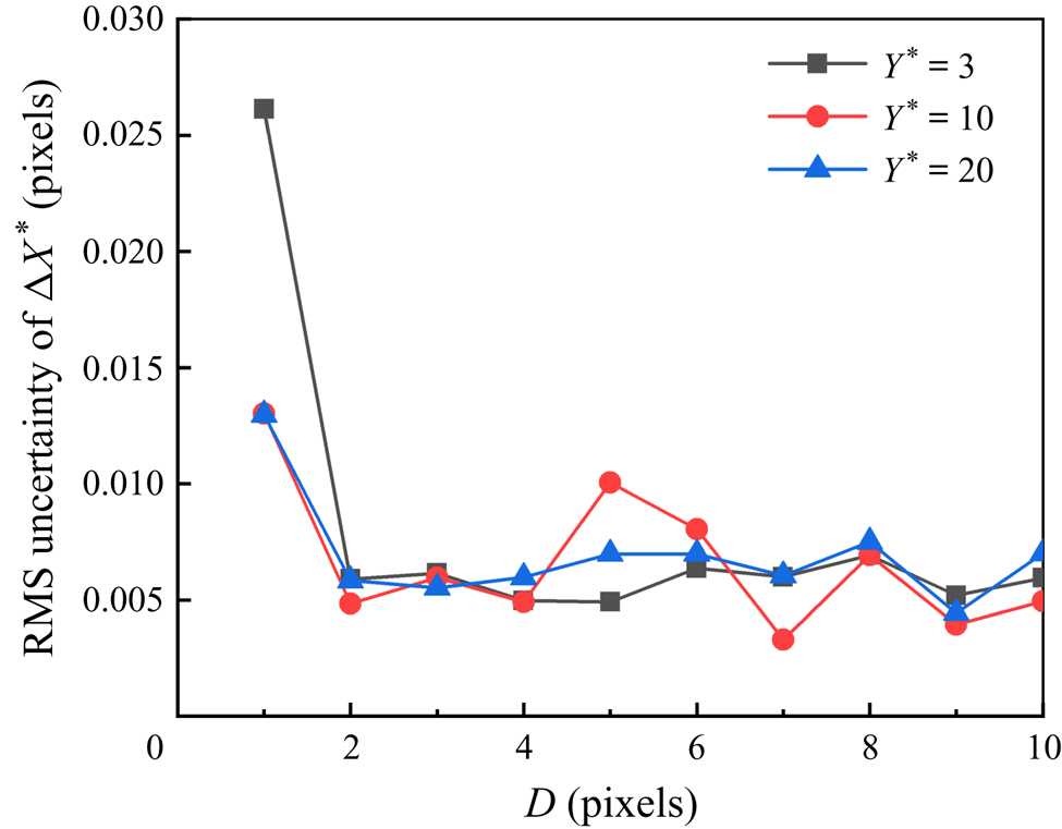
 $n = 5$. Figure 14 shows the root-mean-square uncertainty of the estimated displacement with
 $Y^*=3$, 10 and 20 using the single-pixel algorithm with different
 $D$ varying from 1 to 10 pixel. Uncertainty
 $\sigma _x$ is less than 0.03 pixels for all
 $D=1,\dots , 10$ pixels. For real experimental particle images,
 $D$ is about 3 pixels and the uncertainty (
 $\sigma _x$) is about 0.006, which is based on synthetic images. It is worth noting that although the measurement uncertainty for examining the real experimental particle images will increase by one order of magnitude compared to that for the synthetic images (Kähler et al. Reference Kähler, Scharnowski and Cierpka2012), it is still one order of magnitude below that of the physical processes as the maximum particle displacement between two adjacent frames in the backflow region is approximately 0.1 pixels. Therefore, the single-pixel algorithm can be well suited to resolve the backflow.
Root-mean-square (RMS) uncertainty of the estimated displacement using the single-pixel algorithm.