1. Introduction
Advection–diffusion problems arise in numerous physical scenarios. An incomplete list includes heat and mass convection, hydrodynamic dispersion, microrheology, electro-, diffuso- and thermophoresis, osmotic motors, advection–diffusion-limited aggregation and nutrition uptake by swimming micro-organisms. The advection–diffusion equation is characterised by having non-constant coefficients, and analytic solutions are generally unavailable even for prescribed flows, where the transported scalar is governed by a linear problem. Exceptions include potential-flow problems in two dimensions, where conformal transformations can be employed (Bazant Reference Bazant2004), as well as simple flows in unbounded domains, where the velocity components are either uniform (Acrivos & Taylor Reference Acrivos and Taylor1962) or first-order polynomials of the Cartesian coordinates (Elrick Reference Elrick1962).
Given the abovementioned obstacles, it is hardly surprising that perturbation methods have played a major role in analysing advection–diffusion problems, yielding useful closed-form expressions, physical insight and access to parametric domains that are numerically challenging. In particular, the limits of small and large Péclet number (
 $\mathit{Pe}$
) – the characteristic advection-to-diffusion ratio – have been studied extensively in many different scenarios (Acrivos & Taylor Reference Acrivos and Taylor1962; Brenner Reference Brenner1963; Choi et al.
Reference Choi, Margetis, Squires and Bazant2005; Leal Reference Leal2007). Alternative useful limits may arise from other aspects of the advection–diffusion problem, an important example being the spatial disparity of a large-Reynolds-number advecting flow field. Here, we consider a singular limit arising from the geometry of the problem. In particular, we wish to study steady advection–diffusion external to a slender body. This scenario is evidently relevant to various problems in heat and mass transport, and also to several problems of current practical interest, such as migration of active particles (‘osmotic motors’) via self-diffusophoresis (Brady Reference Brady2011; Michelin & Lauga Reference Michelin and Lauga2014) and nutrition uptake by swimming bacteria (Magar, Goto & Pedley Reference Magar, Goto and Pedley2003).
Slender-body theory is a well-developed subject that has greatly influenced aerodynamics and microhydrodynamics (especially the study of suspensions and swimming of micro-organsisms). It has been applied successfully to various canonical constant-coefficient equations, including Laplace (Handelsman & Keller Reference Handelsman and Keller1967), Stokes (Batchelor Reference Batchelor1970; Cox Reference Cox1970), Helmholtz (Geer Reference Geer1978) and Maxwell equations (Geer Reference Geer1980). In contrast, the possibility of devising similar schemes for the advection–diffusion equation has been largely overlooked. I presume that this void is related to the following apparent incompatibility. Slender-body approximations are based on knowledge of the fundamental solutions of the equation, whereas for the advection–diffusion equation these are different for each flow field considered, and are known only for very simple flows in unbounded domains. Moreover, when the flow and solute distribution are mutually coupled, the underlying problem is nonlinear and the very notion of a ‘fundamental solution’ requires extra care.
A slender-body scheme for an advection–diffusion problem was nevertheless devised by Romero (Reference Romero1995) for the specific case of irrotational flow with Neumann data prescribed at the body boundary. The assumption of an irrotational flow is inherent in his formulation, in which the existence of a velocity potential is exploited towards applying a ‘Goldstein transformation’ (Goldstein Reference Goldstein1929) to the governing equation and boundary conditions. Romero’s analysis yields the surface distribution of the transported scalar up to an ‘algebraic’
 $O({\it\epsilon})$
error.
The present work is motivated by the pertinence of Stokes flows to numerous present applications involving advection–diffusion problems about small particles. We thus consider the slender-body limit, now assuming a general axisymmetric Stokes flow impermeable to the body; the tangential velocity distribution at the particle surface is assumed to be arbitrary, with irrotational and no-slip Stokes flows, as well as various osmotic-type flows (Anderson Reference Anderson1989), being particular cases. At a fixed distance from the axis, the deviation of the flow field from the far-field uniform stream is small in
 ${\it\epsilon}$
. Then, to leading order, the advection–diffusion equation resembles the far-field constant-coefficient equation encountered in small-Péclet-number analyses (Acrivos & Taylor Reference Acrivos and Taylor1962), and the solution can be constructed as a line distribution of singular solutions representing a source advected by a uniform flow. However, while in irrotational flows the velocity deviation from a uniform stream is algebraically small in
 ${\it\epsilon}$
, for Stokes flows the deviation is in general only logarithmically small. The first logarithmic correction to the governing equation is then forced. In the prescribed-flux scenario studied by Romero (Reference Romero1995), we find his two-term result for the surface distribution to remain valid, though now up to a logarithmic error, instead of an algebraic one. Higher-order logarithmic terms, which vanish in the irrotational-flow case, are shown to depend on the specified surface distribution of tangential velocity. In the Dirichlet problem, where the scalar distribution is prescribed at the surface, the situation is more complicated, as the scheme proceeds indefinitely in logarithmic powers regardless of the details of the prescribed flow. Here too the two leading terms are independent of the flow details.
It appears that slender-body approximations may be applied quite generally to study advection–diffusion problems (see § 5 for a discussion). The applicability of the theory to Stokes flows may turn out to be particularly useful, given the abovementioned topical applications. In the present paper, we apply our results to the classical problem of heat convection from a body held at a fixed temperature. Using our results in the Dirichlet case, we find an asymptotic expansion for the Nusselt number in powers of
 $\ln ^{-1}(1/{\it\epsilon})$
. The expression is tested against a numerical computation, for both irrotational and no-slip Stokes flow.
2. Formulation
We consider the dimensionless advection–diffusion equation
 $$\begin{eqnarray}\mathit{Pe}\,\boldsymbol{u}\boldsymbol{\cdot }\boldsymbol{{\rm\nabla}}c={\rm\nabla}^{2}c\end{eqnarray}$$
in the unbounded fluid domain external to a slender body of revolution fixed in space. In (2.1),
 $c$
is the advected scalar,
 $\mathit{Pe}$
is the Péclet number based on particle length and
 $\boldsymbol{u}$
is an axisymmetric Stokes flow impermeable to the body which approaches at large distances the uniform stream
 $$\begin{eqnarray}\boldsymbol{u}\rightarrow \hat{\boldsymbol{e}}_{z}.\end{eqnarray}$$
The axisymmetric distribution of tangential velocity at the surface is assumed to be arbitrary; it must however be
 $O(1)$
, and vary on the
 $O(1)$
longitudinal scale. It should be noted that standard no-slip Stokes flow and irrotational flow are both particular cases. The latter scenario leads to a unique simplification which will be elucidated a posteriori.
It is convenient to work with cylindrical polar coordinates
 $(r,{\it\phi},z)$
in which the particle boundary is given by
 $$\begin{eqnarray}r={\it\epsilon}{\it\kappa}(z),\quad -1\leqslant z\leqslant 1,\end{eqnarray}$$
where
 ${\it\epsilon}$
is the slenderness parameter and
 ${\it\kappa}(z)$
is an
 $O(1)$
shape function vanishing at
 $z=\pm 1$
. Because of axial symmetry,
 $\boldsymbol{u}=u(r,z)\hat{\boldsymbol{e}}_{r}+w(r,z)\hat{\boldsymbol{e}}_{z}$
. The problem governing
 $c$
is closed by prescribing appropriate boundary conditions. We shall consider two prototypic conditions, namely
 $$\begin{eqnarray}\hat{\boldsymbol{n}}\boldsymbol{\cdot }\boldsymbol{{\rm\nabla}}c=-{\it\epsilon}^{-1}j(z)\quad \text{or}\quad c=h(z),\end{eqnarray}$$
the first corresponding to a prescribed flux (Neumann problem), the second to a prescribed value (Dirichlet problem); it should be noted that, because of linearity, the
 ${\it\epsilon}^{-1}$
scaling of the flux in (2.4) results in no loss of generality. The far field condition is taken as
 $c\rightarrow 0$
, implying that
 $c$
represents an excess quantity. Our goal is to calculate the surface distribution of
 $c$
given Neumann data, and the flux distribution
 $\hat{\boldsymbol{n}}\boldsymbol{\cdot }\boldsymbol{{\rm\nabla}}c$
given Dirichlet data.
3. Slender-body limit
In what follows we consider the limit where
 ${\it\epsilon}\ll 1$
with
 $\mathit{Pe}=O(1)$
. This limit is spatially nonuniform, and we treat it in the usual way by decomposing the fluid domain into ‘inner’ and ‘outer’ regions.
3.1. Inner limit:
 ${\it\epsilon}\rightarrow 0$
with
${\it\rho}={\it\epsilon}^{-1}r$
fixed,
$-1<z<1$


Introducing the inner variable
 ${\it\rho}={\it\epsilon}^{-1}r$
, (2.1) becomes
 $$\begin{eqnarray}\mathit{Pe}\left({\it\epsilon}^{-1}u\frac{\partial c}{\partial {\it\rho}}+w\frac{\partial c}{\partial z}\right)={\it\epsilon}^{-2}\frac{1}{{\it\rho}}\frac{\partial }{\partial {\it\rho}}\left({\it\rho}\frac{\partial c}{\partial {\it\rho}}\right)+\frac{\partial ^{2}c}{\partial z^{2}},\end{eqnarray}$$
while conditions (2.4), now applying at
 ${\it\rho}={\it\kappa}(z)$
, read
 $$\begin{eqnarray}\left(\frac{\partial c}{\partial {\it\rho}}-{\it\epsilon}^{2}\frac{\text{d}{\it\kappa}}{\text{d}z}\frac{\partial c}{\partial z}\right)\left[1+O({\it\epsilon}^{2})\right]=-j(z)\quad \text{or}\quad c=h(z).\end{eqnarray}$$
From impermeability,
 $u\sim O({\it\epsilon}w)$
, with
 $w$
at most
 $O(1)$
. As the advection terms in (3.1) are negligible, integration in conjunction with (3.2) yields
 $$\begin{eqnarray}c\sim -{\it\kappa}(z)j(z)\ln {\it\rho}+A(z;{\it\epsilon})+O({\it\epsilon}^{2}),\quad c\sim h(z)+B(z;{\it\epsilon})\ln \frac{{\it\rho}}{{\it\kappa}(z)}+O({\it\epsilon}^{2})\end{eqnarray}$$
in the Neumann and Dirichlet cases respectively. The functions
 $A,B$
, to be determined from matching, may depend logarithmically on
 ${\it\epsilon}$
. Suitable expansions will be seen to be
 $$\begin{eqnarray}A(z;{\it\epsilon})\sim \ln \frac{1}{{\it\epsilon}}A_{-1}(z)+A_{0}(z)+\cdots \,,\quad B(z;{\it\epsilon})\sim \frac{1}{\ln {\displaystyle \frac{1}{{\it\epsilon}}}}B_{1}(z)+\frac{1}{\ln ^{2}{\displaystyle \frac{1}{{\it\epsilon}}}}B_{2}(z)+\cdots \,.\end{eqnarray}$$
3.2. Outer limit:
${\it\epsilon}\rightarrow 0$
with
$r$
fixed


In this limit, the body appears as a finite line segment, and the deviation of
 $\boldsymbol{u}$
from (2.2) is asymptotically small in
 ${\it\epsilon}$
. In fact, from slender-body theory of Stokes flow (Cox Reference Cox1970) we have
 $$\begin{eqnarray}\boldsymbol{u}\sim \hat{\boldsymbol{e}}_{z}+\frac{1}{\ln {\displaystyle \frac{1}{{\it\epsilon}}}}\boldsymbol{u}_{1}(\boldsymbol{x})+\cdots \,.\end{eqnarray}$$
This suggests the outer ansatz
 $$\begin{eqnarray}c\sim {\it\delta}({\it\epsilon})\left[c_{0}(\boldsymbol{x})+\frac{1}{\ln {\displaystyle \frac{1}{{\it\epsilon}}}}c_{1}(\boldsymbol{x})+\cdots \,\right]\!,\end{eqnarray}$$
where, alluding to the purely diffusive slender-body problem (Hinch Reference Hinch1991),
 ${\it\delta}=1$
in the Neumann problem and
 ${\it\delta}=1/\text{ln}(1/{\it\epsilon})$
in the Dirichlet problem. With these definitions, we find at leading order
 $$\begin{eqnarray}\mathit{Pe}\frac{\partial c_{0}}{\partial z}={\rm\nabla}^{2}c_{0},\end{eqnarray}$$
a constant-coefficient equation familiar from small-Péclet-number analyses (Acrivos & Taylor Reference Acrivos and Taylor1962). In those analyses, this equation describes the asymptotic far field, where the body shrinks to a point. Accordingly, the specific solution
 $$\begin{eqnarray}\frac{1}{4{\rm\pi}|\boldsymbol{x}|}\text{e}^{\mathit{Pe}(z-|\boldsymbol{x}|)/2},\end{eqnarray}$$
which represents a source at the origin advected by a uniform stream in the
 $\hat{\boldsymbol{e}}_{z}$
direction, is found to be sufficient for leading-order matching. Analogously, in our outer region the body appears as a line segment. We therefore attempt a solution in the form
 $$\begin{eqnarray}c_{0}=\frac{\text{e}^{\mathit{Pe}\,z/2}}{4{\rm\pi}}\int _{-1}^{1}\frac{m({\it\xi})\text{e}^{-(1/2)\mathit{Pe}\sqrt{(z-{\it\xi})^{2}+r^{2}}}}{\sqrt{(z-{\it\xi})^{2}+r^{2}}}\text{d}{\it\xi},\end{eqnarray}$$
where
 $m(z)\!\exp (\mathit{Pe}\,z/2)$
is the source density per unit length. We note for later reference that for
 $r\ll 1$
,
 $$\begin{eqnarray}c_{0}\sim \frac{\text{e}^{\mathit{Pe}\,z/2}}{4{\rm\pi}}\left[2m(z)\ln \frac{2(1-z^{2})^{1/2}}{r}+\int _{-1}^{1}\frac{m({\it\xi})\text{e}^{-\mathit{Pe}|z-{\it\xi}|/2}-m(z)}{|z-{\it\xi}|}\text{d}{\it\xi}\right],\end{eqnarray}$$
the correction being algebraically small in
 $r$
. This approximation is derived by subtracting and adding
 $m(z)$
to the numerator in (3.9), resulting in two integrals, one singular and one regular as
 $r\rightarrow 0$
. The former is evaluated in closed form and expanded to give the first term in (3.10); the latter limits to the integral in (3.10).
Substituting (3.5) and (3.6) into (2.1), we find that
 $c_{1}$
is governed by the forced equation
 $$\begin{eqnarray}{\rm\nabla}^{2}c_{1}-\mathit{Pe}\frac{\partial c_{1}}{\partial z}=\mathit{Pe}\,\boldsymbol{u}_{1}\boldsymbol{\cdot }\boldsymbol{{\rm\nabla}}c_{0}.\end{eqnarray}$$
In appendix A, we consider the small-
 $r$
behaviour of the forcing term on the right-hand side of (3.11), and conclude that
 $$\begin{eqnarray}c_{1}(r,z)\sim {\hat{c}}(z)\ln r+O(1)\quad \text{as }r\rightarrow 0,\end{eqnarray}$$
wherein
 ${\hat{c}}(z)$
is to obtained via asymptotic matching. Once
 ${\hat{c}}$
is so determined, (3.11) may in principle be solved for
 $c_{1}$
with (3.12) as a boundary condition, in addition to attenuation at large distances. In the prescribed-flux case we shall find from matching that
 ${\hat{c}}\equiv 0$
; this corresponds to adding a homogenous solution in the form (3.9), which has a
 $\ln r$
singularity, such as to cancel the comparable singularity associated with the forcing in (3.11).
Matching can now be performed to determine the two leading terms in the inner expansion. We will find that the leading inner term is independent of the outer one (and could have in fact been guessed from scaling arguments); this leading inner term then determines the leading outer term by fixing
 $m(z)$
, which in turn determines the first correction in the inner region. Finally, the inner correction determines
 ${\hat{c}}(z)$
, which can be used in principle to find the logarithmic correction in the outer region, and then in turn a third inner term. We note in passing that according to the jargon of matched asymptotics (Van Dyke Reference Van Dyke1964), our (geometric) inner region formally constitutes an outer region, and conversely.
3.3. Matching
We match the inner and outer expansions by requiring them to coincide in an overlap domain, represented by the intermediate limit where
 ${\it\eta}={\it\epsilon}^{-{\it\alpha}}r$
(
 $0<{\it\alpha}<1$
) is fixed with
 ${\it\epsilon}\rightarrow 0$
. In this domain, the inner expansions for the Nuemann and Dirichlet problems respectively read
 $$\begin{eqnarray}\displaystyle & \displaystyle c\sim -{\it\kappa}(z)j(z)\ln {\it\eta}+({\it\alpha}-1){\it\kappa}(z)j(z)\ln \frac{1}{{\it\epsilon}}+A(z;{\it\epsilon}), & \displaystyle\end{eqnarray}$$
 $$\begin{eqnarray}\displaystyle & \displaystyle c\sim h(z)+B(z;{\it\epsilon})\left[\ln \frac{{\it\eta}}{{\it\kappa}(z)}+(1-{\it\alpha})\ln \frac{1}{{\it\epsilon}}\right]. & \displaystyle\end{eqnarray}$$
 $$\begin{eqnarray}\displaystyle & & \displaystyle \displaystyle \sim {\it\delta}({\it\epsilon})\frac{\text{e}^{\mathit{Pe}\,z/2}}{4{\rm\pi}}\left[2{\it\alpha}m(z)\ln \frac{1}{{\it\epsilon}}+2m(z)\ln \frac{2(1-z^{2})^{1/2}}{{\it\eta}}\right.\nonumber\\ \displaystyle & & \displaystyle \displaystyle \quad +\,\left.\int _{-1}^{1}\frac{m({\it\xi})\text{e}^{-\mathit{Pe}|z-{\it\xi}|/2}-m(z)}{|z-{\it\xi}|}\text{d}{\it\xi}+o(1)\right]+{\it\delta}({\it\epsilon})\left[-{\it\alpha}{\hat{c}}(z)+O\!\left(\frac{1}{\ln {\displaystyle \frac{1}{{\it\epsilon}}}}\right)\right].\qquad\end{eqnarray}$$
3.3.1. Neumann problem
We recall that here
 ${\it\delta}=1$
. Matching at leading
 $O(\ln 1/{\it\epsilon})$
we find
 $$\begin{eqnarray}A_{-1}(z)={\it\kappa}(z)j(z),\quad m(z)=2{\rm\pi}{\it\kappa}(z)j(z)\text{e}^{-\mathit{Pe}\,z/2}.\end{eqnarray}$$
Matching at
 $O(1)$
yields
 $$\begin{eqnarray}A_{0}(z)={\it\kappa}(z)j(z)\ln 2(1-z^{2})^{1/2}+\frac{1}{2}\int _{-1}^{1}\frac{{\it\kappa}({\it\xi})j({\it\xi})\text{e}^{\mathit{Pe}\left(z-{\it\xi}-|z-{\it\xi}|\right)/2}-{\it\kappa}(z)j(z)}{|z-{\it\xi}|}\text{d}{\it\xi},\end{eqnarray}$$
together with
 $$\begin{eqnarray}{\hat{c}}(z)=0,\end{eqnarray}$$
the latter following from the absence of an inner
 $O(1)$
term depending on
 ${\it\alpha}$
. Referring back to (3.1), we have determined the surface distribution of
 $c$
up to
 $O(1)$
,
 $$\begin{eqnarray}\displaystyle c & {\sim} & \displaystyle {\it\kappa}(z)j(z)\ln \frac{2(1-z^{2})^{1/2}}{{\it\epsilon}{\it\kappa}(z)}\nonumber\\ \displaystyle & & \displaystyle +\,\frac{1}{2}\int _{-1}^{1}\frac{{\it\kappa}({\it\xi})j({\it\xi})\text{e}^{\mathit{Pe}\left(z-{\it\xi}-|z-{\it\xi}|\right)/2}-{\it\kappa}(z)j(z)}{|z-{\it\xi}|}\text{d}{\it\xi}+O\!\left(\frac{1}{\ln {\displaystyle \frac{1}{{\it\epsilon}}}}\right).\end{eqnarray}$$
This expression agrees with Romero (Reference Romero1995), apart from the logarithmic error (see § 3.4).
3.3.2. Dirichlet problem
We recall that here
 ${\it\delta}=\ln ^{-1}(1/{\it\epsilon})$
. Matching at
 $O(1)$
we find
 $$\begin{eqnarray}B_{1}(z)=-h(z),\quad m(z)=2{\rm\pi}h(z)\text{e}^{-\mathit{Pe}\,z/2}.\end{eqnarray}$$
Matching at
 $O(\ln ^{-1}1/{\it\epsilon})$
yields
 $$\begin{eqnarray}B_{2}(z)=h(z)\ln \frac{2(1-z^{2})^{1/2}}{{\it\kappa}(z)}+\frac{1}{2}\int _{-1}^{1}\frac{h({\it\xi})\text{e}^{\mathit{Pe}\left(z-{\it\xi}-|z-{\it\xi}|\right)/2}-h(z)}{|z-{\it\xi}|}\text{d}{\it\xi},\end{eqnarray}$$
together with
 $$\begin{eqnarray}{\hat{c}}(z)=B_{2}(z).\end{eqnarray}$$
Referring back to (3.1), we find the expansion
 $$\begin{eqnarray}\hat{\boldsymbol{n}}\boldsymbol{\cdot }\boldsymbol{{\rm\nabla}}c\sim \frac{1}{{\it\kappa}(z){\it\epsilon}\ln {\displaystyle \frac{1}{{\it\epsilon}}}}\left[B_{1}(z)+\frac{1}{\ln {\displaystyle \frac{1}{{\it\epsilon}}}}B_{2}(z)+O\!\left(\frac{1}{\ln ^{2}{\displaystyle \frac{1}{{\it\epsilon}}}}\right)\right]\end{eqnarray}$$
for the surface flux density.
3.4. The case of irrotational flow
In the special case of irrotational flow, the deviation of the velocity field from the uniform stream is, for fixed
 $r$
,
 $O({\it\epsilon}^{2}\ln {\it\epsilon})$
(Hinch Reference Hinch1991). The outer solution is then given by (3.9) to algebraic order, with
 $m$
now having an expansion in powers of
 $1/\text{ln}(1/{\it\epsilon})$
. In the Neumann case, matching shows that only the leading term in this expansion is required. The error in (3.19) is then reduced to an algebraic one, as in Romero (Reference Romero1995). In the Dirichlet problem, the expansion of
 $m$
is infinite. It should be noted that in both the Neumann and Dirichlet problems, the relative difference in the inner solute concentration between the cases of no-slip and irrotational flows is
 $O(\ln ^{-2}(1/{\it\epsilon}))$
, see (3.19) and (3.23).
4. Forced heat convection from a slender body
The above formulae can be applied to a variety of physical scenarios. As an example, consider the classical problem of forced heat convection from an isothermal body. The problem conforms to our dimensionless formulation in the Dirichlet case upon defining
 $c=(T-T_{\infty })/(T_{s}-T_{\infty })$
,
 $h(z)\equiv 1$
and
 $\mathit{Pe}={\mathcal{U}}l/D$
, where
 $T$
is the temperature field,
 $T_{\infty }$
is the temperature far away from the body,
 ${\mathcal{U}}$
is the magnitude of the far-field stream,
 $2l$
is the body length and
 $D=k/{\it\rho}C_{p}$
is the heat diffusivity (
 $k$
being the heat conductivity,
 ${\it\rho}$
the fluid density and
 $C_{p}$
the heat capacity). Lengths are normalised by
 $l$
. The quantity of interest is the Nusselt number, the normalised total flux (Leal Reference Leal2007)
 $$\begin{eqnarray}\mathit{Nu}=-\frac{2}{{\mathcal{A}}}\oint \hat{\boldsymbol{n}}\boldsymbol{\cdot }\boldsymbol{{\rm\nabla}}c\text{d}A,\end{eqnarray}$$
where
 ${\mathcal{A}}$
is the dimensionless surface area of the body and
 $\text{d}A$
is a dimensionless area element. Our interest lies in the ratio
 $\mathit{Nu}({\it\epsilon},\mathit{Pe})/\mathit{Nu}({\it\epsilon},0)$
as
 ${\it\epsilon}\rightarrow 0$
, which describes the effectiveness of advection as the body becomes slender.
From (3.23),
 $$\begin{eqnarray}\displaystyle & & \displaystyle -\oint \hat{\boldsymbol{n}}\boldsymbol{\cdot }\boldsymbol{{\rm\nabla}}c\text{d}A\sim \frac{4{\rm\pi}}{\ln {\displaystyle \frac{1}{{\it\epsilon}}}}-\frac{2{\rm\pi}}{\ln ^{2}{\displaystyle \frac{1}{{\it\epsilon}}}}\left[\mathop{\int }_{-1}^{1}\ln \frac{2(1-z^{2})^{1/2}}{{\it\kappa}(z)}\text{d}z\right.\nonumber\\ \displaystyle & & \displaystyle \quad \left.+\,\frac{1}{2}\int _{-1}^{1}\int _{-1}^{1}\frac{\text{e}^{\mathit{Pe}(z-{\it\xi}-|z-{\it\xi}|)/2}-1}{|z-{\it\xi}|}\text{d}{\it\xi}\text{d}z\right]+O\!\left(\frac{1}{\ln ^{3}{\displaystyle \frac{1}{{\it\epsilon}}}}\right)\end{eqnarray}$$
as
 ${\it\epsilon}\rightarrow 0$
. Evaluating the double integral, we find
 $$\begin{eqnarray}\frac{\mathit{Nu}({\it\epsilon},\mathit{Pe})}{\mathit{Nu}({\it\epsilon},0)}\sim 1+\frac{g(\mathit{Pe})}{2\ln {\displaystyle \frac{1}{{\it\epsilon}}}}+O\!\left(\frac{1}{\ln ^{2}{\displaystyle \frac{1}{{\it\epsilon}}}}\right),\end{eqnarray}$$
where
 $$\begin{eqnarray}g(\mathit{Pe})=\ln (2\mathit{Pe})-1+{\it\gamma}-\text{Ei}(-2\mathit{Pe})-\frac{1}{2\mathit{Pe}}\left(\text{e}^{-2\mathit{Pe}}-1\right),\end{eqnarray}$$
in which
 ${\it\gamma}\approx 0.577$
is the Euler–Gamma constant and
 $\text{Ei}$
is the exponential-integral function. The ratio (4.3) is notably independent of the shape function
 ${\it\kappa}(z)$
up to the order calculated. At small and large
 $\mathit{Pe}$
respectively,
 $$\begin{eqnarray}g\sim \mathit{Pe}+O(\mathit{Pe}^{2}),\quad g\sim \ln (2\mathit{Pe})-1+{\it\gamma}+O\!\left(\frac{1}{\mathit{Pe}}\right).\end{eqnarray}$$
Thus, at moderately large Péclet numbers,
 $1\ll \mathit{Pe}\ll {\it\epsilon}^{-1}$
, expansion (4.3) is
 ${\sim}1+\ln \mathit{Pe}/2\ln (1/{\it\epsilon})$
, describing a very slow growth of heat flux with increasing advection.
It is illuminating to compare (4.3) with small-Péclet-number theory, in particular with the expansion
 $$\begin{eqnarray}\frac{\mathit{Nu}({\it\epsilon},\mathit{Pe})}{\mathit{Nu}({\it\epsilon},0)}\sim 1+\frac{1}{8{\rm\pi}}Q_{0}\mathit{Pe}+\frac{1}{8{\rm\pi}}Q_{0}\,f\,\mathit{Pe}^{2}\ln \mathit{Pe}+O(\mathit{Pe}^{2})\end{eqnarray}$$
derived by Brenner (Reference Brenner1963) for a particle of arbitrary shape in an arbitrary creeping flow. Here,
 $Q_{0}$
denotes the dimensionless flux (4.2) at
 $\mathit{Pe}=0$
and
 $f$
is the hydrodynamic force on the body normalised by
 $6{\rm\pi}{\it\mu}l\,{\mathcal{U}}$
,
 ${\it\mu}$
being the viscosity of the fluid. While it is not a priori guaranteed that the singular limits of small
 $\mathit{Pe}$
and small
 ${\it\epsilon}$
commute, we actually find agreement at least up to
 $O(\mathit{Pe}\ln ^{-1}(1/{\it\epsilon}))$
when comparing with the small-
 ${\it\epsilon}$
limit of (4.6). Furthermore, noting that for Stokes flow
 $f\sim O(1/\text{ln}(1/{\it\epsilon}))$
, the small-
 ${\it\epsilon}$
limit of the
 $\mathit{Pe}^{2}\ln \mathit{Pe}$
term in (4.6) becomes
 $O(\mathit{Pe}^{2}\ln \mathit{Pe}/\text{ln}^{2}(1/{\it\epsilon}))$
. While we did not calculate
 $O(1/\text{ln}^{2}(1/{\it\epsilon}))$
terms, our scheme implies that this is indeed the first order where the surface flux depends upon the specific details of the Stokes flows considered, and hence upon
 $f$
.
4.1. Comparison with numerics
The error in (4.3) is logarithmically small in
 ${\it\epsilon}$
. This sheds doubt on the applicability of the result to mildly small
 ${\it\epsilon}$
. We wish to test this via a comparison with a numerical solution of the forced convection problem about a prolate spheroid, for both irrotational and no-slip Stokes flows. The solution was obtained by approximating the advection–diffusion equation using second-order central differences in prolate spheroidal coordinates, with the transverse coordinate transformed such that sufficient nodes were distributed near the surface. The far-field condition employed was of the form (3.8), with the strength of the source iteratively adjusted according to the total flux found from integration. The resulting ratio
 $\mathit{Nu}({\it\epsilon},\mathit{Pe})/\mathit{Nu}({\it\epsilon},0)$
is plotted in figure 1 for
 ${\it\epsilon}=0.1$
and
 ${\it\epsilon}=0.01$
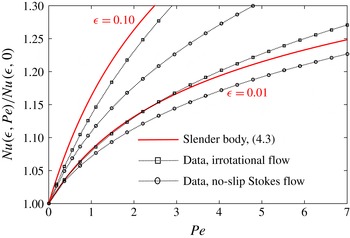
; the squares and circles respectively correspond to the cases of irrotational and no-slip Stokes flow. The red lines correspond to the slender-body approximation (4.3). The agreement is arguably good considering the logarithmic error anticipated.
The Nusselt number for forced heat convection over a slender prolate spheroid (
 ${\it\epsilon}=0.1,0.01$
), normalised by its value at
 $\mathit{Pe}=0$
. The red lines correspond to the asymptotic slender-body approximation (4.3). The symbols show values obtained from a numerical computation for irrotational (squares) and no-slip Stokes (circles) flows; the dotted lines connecting the symbols are intended to help to distinguish between the data sets.

5. Discussion
We have analysed advective–diffusive transport about a slender body of revolution situated in an axisymmetric Stokes flow. The scheme yields a bidirectional mapping between Neumann and Dirichlet conditions at the body boundary which is asymptotic in the slenderness parameter
 ${\it\epsilon}$
. In general, the error is logarithmic in
 ${\it\epsilon}$
, an exception being the unique scenario studied by Romero (Reference Romero1995), where the flow is irrotational and Neumann conditions are prescribed. For the sake of illustration, the Dirichlet-to-Neumann mapping was applied to the classical problem of heat convection from a body held at a fixed temperature. The resulting expansion for the average Nusselt number was found to agree favourably with a numerical computation, especially when considering that the error is logarithmic.
A key feature of the slender-body scheme is that it is not limited to small values of the Péclet number. A question arises whether the scheme continues to hold for
 $\mathit{Pe}\gg 1$
. By inspection of the inner equation (3.1) we see that advection remains subdominant as long as
 $\mathit{Pe}\ll {\it\epsilon}^{-2}$
. A more stringent bound however arises a posteriori by considering the large-
 $\mathit{Pe}$
behaviour of the terms in our expansions; for example, expansion (4.3) for the Nusselt number loses asymptoticness when
 $\mathit{Pe}\sim O(1/{\it\epsilon})$
. In the latter limit, advection dominates the outer region (hence
 $c$
is exponentially small in
 $\mathit{Pe}$
), while diffusion still dominates the inner region. An intermediate layer forms where diffusion and advection are balanced. In the distinguished limit
 $\mathit{Pe}\sim O({\it\epsilon}^{-2})$
, advection becomes important in the inner region, whereby this region effectively coalesces with the intermediate layer. Finally, in the extreme scenario
 $\mathit{Pe}\gg {\it\epsilon}^{-2}$
, advection dominates the inner region, and the intermediate layer transforms into an internal boundary layer. The latter case is expected to be similar to traditional boundary-layer analyses at large Péclet numbers, where only a single length scale characterising the body is assumed (Leal Reference Leal2007).
The present analysis can be generalised to flows approaching a uniform stream that is oblique to the body centreline. The diffusion-dominated inner region remains axisymmetric, while the outer solution is constructed similarly, but with the exponent
 $z-|\boldsymbol{x}|$
in (3.8) replaced by
 $\hat{\boldsymbol{e}}\boldsymbol{\cdot }\boldsymbol{x}-|\boldsymbol{x}|$
(
 $\hat{\boldsymbol{e}}$
being a unit vector in the direction of the far-field stream). Slender bodies of non-axisymmetric shape can also be considered by applying a conformal map to the inner region (Hinch Reference Hinch1991). Another immediate extension would be to consider ‘mixed’, or even nonlinear, boundary conditions. A question of greater generality is whether the approach can be applied to flows that do not approach a uniform stream. The answer is in the affirmative, on the condition that we can find the fundamental solution of the advection–diffusion equation in an unbounded domain with the velocity field reduced to its leading-order outer limit, i.e.
 $r$
fixed with
 ${\it\epsilon}\rightarrow 0$
. Any flow approaching a simple shear profile is an example (Leal Reference Leal2007). To conclude, it is not the equation itself that determines whether a slender-body approximation can be devised, but rather the simplicity of its outer limit. With this in mind, there is no real obstacle in tackling nonlinear equations. For example, the outer limit in the moderate-Reynolds-number flow over a slender body is just Oseen’s equation, whereby a solution can be obtained as a line distribution of Oseen-type point forces (Homentcovschi Reference Homentcovschi1981).
Appendix A. The behaviour of
$c_{1}$
as
$r\rightarrow 0$


Equation (3.11) is rewritten as
 $$\begin{eqnarray}\frac{1}{r}\frac{\partial }{\partial r}\left(r\frac{\partial c_{1}}{\partial r}\right)+\frac{\partial ^{2}c_{1}}{\partial z^{2}}-\mathit{Pe}\frac{\partial c_{1}}{\partial z}=\mathit{Pe}\,\left(u_{1}\frac{\partial c_{0}}{\partial r}+w_{1}\frac{\partial c_{0}}{\partial z}\right).\end{eqnarray}$$
Consider the behaviour of the right-hand-side forcing as
 $r\rightarrow 0$
. The
 $(r,z)$
components of the logarithmic velocity deviation
 $\boldsymbol{u}_{1}$
may be written as (Cox Reference Cox1970)
 $$\begin{eqnarray}\displaystyle & \displaystyle u_{1}(r,z)=-\frac{r}{4}\int _{-1}^{1}\frac{(z-{\it\xi})(1-w_{s}({\it\xi}))}{\left[r^{2}+(z-{\it\xi})^{2}\right]^{3/2}}\text{d}{\it\xi}, & \displaystyle\end{eqnarray}$$
 $$\begin{eqnarray}\displaystyle & \displaystyle w_{1}(r,z)=-\frac{1}{4}\int _{-1}^{1}\frac{1-w_{s}({\it\xi})}{\left[r^{2}+(z-{\it\xi})^{2}\right]^{1/2}}\text{d}{\it\xi}-\frac{1}{4}\int _{-1}^{1}\frac{(z-{\it\xi})^{2}(1-w_{s}({\it\xi}))}{\left[r^{2}+(z-{\it\xi})^{2}\right]^{3/2}}\text{d}{\it\xi}, & \displaystyle\end{eqnarray}$$
 $w_{s}(z)$
is, to
 $O({\it\epsilon})$
, the
 $z$
component of the tangential velocity relative to the uniform stream prescribed at the surface: for no-slip flow,
 $w_{s}\equiv 0$
; for irrotational flow, where the deviation
 $\boldsymbol{u}_{1}$
vanishes (Hinch Reference Hinch1991),
 $w_{s}\equiv 1$
. The small-
 $r$
expansions of (A 2) and (A 3) are obtained by integration by parts in conjunction with the method leading to (3.10). One finds
 $$\begin{eqnarray}u_{1}\sim {\textstyle \frac{1}{2}}w_{s}^{\prime }(z)r\ln r+O(r),\quad w_{1}\sim \left[1-w_{s}(z)\right]\ln r+\tilde{w}_{1}(z)+o(1),\end{eqnarray}$$
with
 $\tilde{w}_{1}(z)$
a function depending on
 ${\it\kappa}(z)$
. From (3.10) we find
 $$\begin{eqnarray}\frac{\partial c_{0}}{\partial r}\sim k_{1}(z)\frac{1}{r}+O(1),\quad \frac{\partial c_{0}}{\partial z}\sim k_{2}(z)\ln r+k_{3}(z)+o(1),\end{eqnarray}$$
where the functions
 $k_{1}(z),k_{2}(z)$
and
 $k_{3}(z)$
are known once
 $m(z)$
is determined. Thus,
 $$\begin{eqnarray}\displaystyle & & \displaystyle \boldsymbol{u}_{1}\boldsymbol{\cdot }\boldsymbol{{\rm\nabla}}c_{0}\sim \left[w_{s}(z)-1\right]k_{2}(z)\ln ^{2}r\nonumber\\ \displaystyle & & \displaystyle \quad +\,\left\{\tilde{w}_{1}(z)k_{2}(z)+{\textstyle \frac{1}{2}}w_{s}^{\prime }(z)k_{1}(z)-\left[1-w_{s}(z)\right]k_{3}(z)\right\}\ln r+O(1).\end{eqnarray}$$
The result (3.12) now follows from consideration of the possible small-
 $r$
balances of (A 1), assuming that
 $\partial /\partial z\sim O(1)$
. First, it should be noted that
 $c_{1}$
cannot be
 $O(\ln ^{2}r)$
or larger, since then the radial operator
 $\mathscr{L}_{r}=r^{-1}\partial _{r}\left(r\partial _{r}\right)$
in (A 1) is unbalanced. A singular
 $O(\ln r)$
term, where
 $c_{1}\sim {\hat{c}}(z)\ln r$
, is however possible: the leading
 $O(\ln ^{2}r)$
forcing term is balanced by the action of
 $\mathscr{L}_{r}$
on a high-order term, and at
 $O(\ln r)$
we have a balance between the
 $\ln r$
forcing term, the
 $z$
derivatives
 $\text{d}^{2}{\hat{c}}/\text{d}^{2}z-\mathit{Pe}\,\text{d}{\hat{c}}/\text{d}z$
and perhaps also the action of
 $\mathscr{L}_{r}$
on a high-order term (note that
 $\mathscr{L}_{r}(\ln r)=0$
). Thus (3.12) represents the most singular behaviour allowed. We stress that a regular solution, where
 ${\hat{c}}=0$
, is also possible; indeed, we can always construct a homogenous solution similar to (3.9) such that the
 $\ln r$
singularity triggered by the forcing is eliminated. This is actually the case in the Neumann problem, see (3.18).