Introduction
Software subroutines can be viewed as a frozen theory of how design intention is computed under certain logic. Therefore, issues on CAD operation for analyzing structural design might occur in the discrepancy between the way the user and the subroutines represent the design intention. In Vitruvius Redux, Mitchell outlines the limit of Durand's enumerative object-oriented iteration and its digital embodiment in BIM software. In this software, objects and combinatorial searches allow for an effective design modeling process; however, the provided objects (e.g. roof, wall, and door tools) are constrained by well-known typologies and may not fully align with the designer intention. Reflecting on several structural design cases, Mitchell called for re-promoting the parametric-grammatical approach with a shape grammar embedding mechanism for its impartiality to typological constraints (Mitchell, Reference Mitchell1998, Reference Mitchell, Antonsson and Cagan2001). This paper sheds lights on representational issues in structural design from where Mitchell left off.
In physical media, structural problems are represented with a set of physical variables (e.g. material, loading, and supporting elements). Physical behavior on one scale is assumed to resemble that of another scale as the load-stress distribution is considered proportional across scales. For instance, experimental models developed by Gaudi, Otto and Isler (e.g. soap film, chains, and fabrics) served as physical schemas to simulate the behavior of shapes on a larger scale, such as a wide-span roof or a bridge (Collins, Reference Collins1963; Otto, Reference Otto1973; Chilton & Isler, Reference Chilton and Isler2000). By modifying the loads, supports, and material, the physical model could provide immediate feedback in an attempt to find desirable forms.
In digital media, structural analysis tools represent physical shapes into an assemblage of finite vertices, edges, and faces, along with their mechanical descriptions (e.g. a force's magnitude and the vertices’ degree of freedom). The shapes’ physical behavior is then simulated through virtual equilibrium modeling, either numerically, for instance with the finite element method, or graphically, such as in graphic statics (Maxwell, Reference Maxwell1864; Rankine, Reference Rankine1864; Cremona, Reference Cremona1885; Przemieniecki, Reference Przemieniecki1985; Bathe, Reference Bathe1996). Through this process, structural software, including programs such as Adina, Ansys, and Formfinder; add-ons, such as Karamba3D, RhinoVAULT, SOFiSTiK, and Revit Structure; and web-based apps, such as StructureFIT and eQUILIBRIUM, allow users to virtually analyze, simulate, and optimize an object's structural behavior (Bathe & Larsson, Reference Bathe and Larsson1986; Azhar et al., Reference Azhar, Nadeem, Mok and Leung2008; Rippmann et al., Reference Rippmann, Lachauer and Block2012; Mueller & Ochsendorf, Reference Mueller and Ochsendorf2013; Preisinger & Heimrath, Reference Preisinger and Heimrath2014).
Operating in virtual space, the structural software provides more freedom and flexibility to manipulate and simulate the design's structural behavior without the laborious tasks often required in a physical simulation (e.g. preparing physical models and testing equipments). Despite these advantages, it seems that association with existing physical precedents remains strongly bounded, as similar structural topologies keep recurring from the software. One popular example is the mesh-relaxation strategy used to simulate an object's deformation (e.g. membrane) under a certain load. This inclination toward a particular topology recalls Mitchell's concern, in that the objects provided in a software could lead to similar outputs across different projects. However, most structural software does not provide topological objects other than the basic structural elements and mechanical laws to run the structural simulations. Except for a few apps equipped with templates for learning (e.g. tower, bridge, and dome templates), structural software mostly lets the user model the structural problem and constraint the topology themselves.
Nevertheless, the analytical method underlying the software's subroutines does have specific ways of representing the design model. Some methods ask for a static model as an input, while others allow for a parametric model. This condition implies that topological similarities from structural software could be contributed partly by the software's subroutines and partly by the user's perception in representing the design problem to the software.
This study aims to investigate the way in which a structural problem is perceived and represented in order to identify their consequences and opportunities in design. In this case, we use shape grammar schema to contrast two widely used analytical methods: Finite-Element Analysis (FEM) and Graphic Statics, as well as their grammatical versions: Shape Annealing and Grammar-based Graphic Statics (Shea et al., Reference Shea, Cagan and Fenves1997; Lee et al., Reference Lee, Fivet, Mueller, Thomsen, Tamke, Gengnagel, Faircloth and Scheurer2015). Findings from this study are formulated into a new method for generating novel structures with less topological constraints.
This paper consists of four sections: first, we explain shape-grammar rule schemas and group them based on the typical modeling procedures in structural software. Second, using the rule schemas, we analyze parametric and grammatical representations of FEM and Graphic Statics. Third, we identify constraints and opportunities arising from such analysis and propose a new method for reasoning and representing shapes in structural design. Fourth, we demonstrate examples of how this new method could generate novel structures with less dependency on existing topologies. We conclude by discussing the role of shape-grammar rule schemas in analyzing and synthesizing representation mechanism in structural design strategy.
This research responds to the current state-of-the-art of shape-grammar rule schemas on investigating structural design problems from both users and software perspectives, including some of the latest developments in grammatical structure. This agenda is well suited to the visual calculation mechanism in shape grammar, as expressed in C′ = [C − t(a)] + t(b). Computing a shape rule a → b demands an intense visual recognition process to match the predicate shape (a) with the initial shape C via transformation t(a), before applying the new shape (b) using transformation t(b) to produce a new shape C′.Footnote 1
Rule schemas
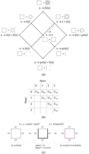
To rationalize various modeling procedures in structural analysis, we schematize their representational mechanisms with shape grammar's rule schemas. As proposed by Stiny in Shape (Reference Stiny2006): “A rule schema x → y is a pair of variable x and y that takes shapes in algebra U ij as values. The values are given in an assignment g that satisfies a predicate (condition). Whenever g is used, a rule g(x) → g(y) is defined. g(x) → g(y) then applies as usual (as shape rule a → b)”. Rule schemas go hand in hand with the algebra of shapes U ij to define a shape based on its space (j) and spatial dimension (i) (Fig. 1b). The subscripts i and j can be 0, 1, 2, or 3; for instance, U 12 is an algebra for a line in a two-dimensional (2D) space. Algebra which has i = 0 are points in space (U 0j), hence they are symbolic and can be directly translated into the discrete operation in a computer, whereas shapes in i > 0 could be perceived as a discrete and continuous shape in a user's perception, and thus they are more user-friendly. Label (V) distinguishes a shape's orientation and belonging by marking it with symbols or parts of the shape (Stiny, Reference Stiny1992). Shape U ij works with an algebra of label V ij, for instance, a label V 12 on a shape U 22 identify an orientation of a 2D shape with a 1D label, such as a line-label embedded in a square's edges.
(a) A lattice showing rule schemas’ relationship with example shape rule (b) Algebra of Shape; (c) an example of descriptive schema iteration on registering physical description on a selected shape.

The interplay between shape rules and rule schemas was discussed by Economou and Kotsopoulos (Reference Economou, Kotsopoulos, Gero and Hanna2015); whereby shape rule, for example,  , provides straightforward visual calculations for a specific shape. Rule schema, for example, x → t(x), offers an abstractions of the rule mechanism that is applicable to different shape rule. They contrasted these differences by exemplifying the way in which different schemas distinguish various ways of seeing a shape, and how one schema translated into different shape rules. Additionally, Economou and Kotsopoulos (Reference Economou, Kotsopoulos, Gero and Hanna2015) also provide annotation for schema development, such as data registration, for example, S 1(L 1, L 2, L 3) and function notation, that is, x → f(x). Rule schema's capacity in encapsulating different shape rules could help to interpret how a user might perceive a structural design from different modeling procedures and vice versa, that is, how one modeling procedure represents different designs.
Groups of schemas
The shape-grammar rule schemas have been used in several contexts where the schemas are grouped to suit different agendas. For example, in assisting students to communicate their ways of thinking in studio projects, Özkar (Reference Özkar2011) classified the schemas into groups for pedagogical purposes, such as a schema for putting two shapes together x → x + t(x) and a schema for a design exercise x → Σt(x). Muslimin (Reference Muslimin2012) grouped the schema based on Gestalt Law principles to re-describe how our visual perception construct a whole from the parts; for instance, a schema for visual constancy x → t −1(x), a schema for visual figuration x → b −1(x), and a schema for visual simplification x → prt−1(x).
For our agenda, we grouped the schemas based on general structural modeling procedures, where the shape needs to be recognized and described with physical attributes before being geometrically or mechanically transformed (Bathe, Reference Bathe1996). The lattice in Figure 1a shows the way the following schemas are structured for our cases (see the introduction of schema lattice in Stiny, Reference Stiny2011).
• Recognition Schema (also known as identity schema) x → x defines a shape that is being visually focused without any mechanical meaning (Stiny, Reference Stiny1993; Krstic, Reference Krstic2001, Reference Krstic2005), while a schema → (without any shape on the left and right sides of the arrow) means do nothing with a shape (Stiny, Reference Stiny1996). The latter allows a shape to be idle in a parallel computation. This type of schemas allows users to embed shapes ambiguously and explore different ways of seeing the same shape before further modification with other schemas. They are centered in the lattice as the basis for the user's visual calculation in each step.
• Transformation Schema let the user transforms the shape according to binary operations with schema x → x + t(x), x → div(x) or x → x′ + x″, and x → y (e.g. addition, subdivision, subtraction, and substitution), and/or formal transformations with schema x → t(x) (e.g. translation, rotation, reflection, and scaling). The former changes the topology by generatively changing the shape during the computation, while the latter constrains the shape topology throughout the computation process. Schema x → Σt(x), at the top of the lattice, repeats the transformation generatively or recursively, such as in fractal geometry.
• Reduction Schema allows the user to retrieve a shape from a different or the same spatial dimension. Boundary schema x → b(x) retrieves a shape's boundary from a lower dimension or a shape's content from a higher dimension x → b −1(x). Part schema, x → prt(x), retrieves the sub-shapes, or the parent-shape with x → prt−1(x) from the same spatial dimension. Schema x → prt(x)I + prt(x)II recognize two different parts of a shape. Boundary and part schemas are connected in the lattice. When t(x) and prt(x) map a shape to itself (e.g. with 360° rotation, or with prt(x) fully occupying the parent shape), t(x) or prt(x) is equal to x. Under such a condition, the schema x → t(x) + b(x) can be simplified into x → x + b(x), and the schema x → t(x) + prt(x) into x → x + prt(x).
• Descriptive Schema registers the shape's attributes with a string function: a ← a[D a(x)], where a symbolizes shape's physical properties, D a is the property's value, and x is a list of shapes to be attributed with a and D a. The left arrow ← specifies property's registration. The shape physical properties are stored in a list (a 1, a 2, a3, … , a n), where a n is a pair of the property's value and the attributed shape(s) (see more about description function in Stiny, Reference Stiny1981). To empty the list, a function a(:) ← a removes all data for property a.
For this case, our descriptive schema adapts parameters from a simple bar problem in FEM analysis, that is, the bar's length (L), sectional area (A), external force (R), supporting condition (S), and material stiffness (E) (Bathe, Reference Bathe1996). Thus, the description list is (L, A, E, R, S) which is equipped with descriptive functions as follows:

The description list can be updated with new data. For example in Figure 1c, applying a function E ← E[1(L2, L3, L4)] will register rigid material into sub-shapes L2, L3, L4 and update the list into {L, A, E[1(L2, L3, L4)], R, S} (in this paper, we simplify the material elasticity's value into D E = 1 means rigid; D E = 0 means flexible).
With descriptive schema, the data and computation history can be recorded for further use, such as for CAD programming or documenting a user's creative process during the computation. This could be a useful companion, as shape grammar computation is memoryless, in the sense that a shape can be perceived as if a user sees the shape for the first time, and attributes in the previous steps can be ignored in the next step.
Parametric and grammatical structure revisited
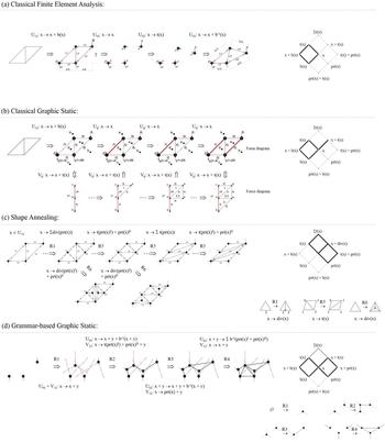
With the group of rule schemas, in the following sections, we interpret the classical FEM and graphic static representations and their grammatical versions, that is, shape annealing and grammar-based graphic statics. To contrast the differences between them, the same initial shape in algebra U 12,  , is used to see how the shape is recognized, described, and transformed under different methods (Fig. 2).
Parametric and Grammatical Structural Synthesis, with the lattice on the right indicating the dominant schemas used in each operation: (a) A Classical Finite Element Analysis procedure on representing a design into an assemblage of discrete lines and vertices. The physical behavior is mathematically simulated in a zero-dimensional space before visualized back into a higher spatial dimension; (b) In Classical Graphic Static, a shape is identified as an assemblage of point, line, and polygon along with the applied forces in a form diagram (first row) and then force diagram is developed accordingly to represent and graphically calculate the force acting on a shape's (second row); (c) Hypothetical Shape Annealing iteration using three of the original rules (Shea & Cagan, Reference Shea and Cagan1997). The initial shape is labeled and embedded with mechanical attributes. (d) Hypothetical Grammatical Graphic Static iteration. Instead of using a predefined design, it started with initial supporting and loading condition on several points. Using a set of rules (Lee et al., Reference Lee, Fivet, Mueller, Thomsen, Tamke, Gengnagel, Faircloth and Scheurer2015), the grammar develops a series of forces lines to be chosen as a predicate shape for the subsequent steps.

Parametric iteration in the classical FEM and graphic statics
Classical FEM
In a simple bar problem in Figure 2a, a physical shape is represented as an assemblage of lines (U 12) before being applied with the mechanical attributes. The process of how the user follows the framework in FEM can be represented with schema x → x + b(x) to return the line's endpoints. Descriptive schemas then register their physical attributes to describe that the scaling factors for all shapes’ lengths and sectional areas are 1 (i.e. no scaling), stiffness for all shapes is 1 (rigid), the force vector applied to a point P1 is −1 (downward), and the support degree of freedoms for points P2 and P3 are 0 (fixed support):
With this registration, the shape's physical behavior is mathematically obtained by equating the internal and external forces based on the principle of virtual equilibrium dP = LR/EA, which transforms the points (P) into new positions (dP), represented with the schema x → t(x). Note that, in this method, the shapes physical behavior is analyzed in the algebra of U 02 (symbolic). Based on the new positions, schema x → x + b −1(x) returns the lines to visualize the simulation results showing the initial line's length (L) changed into L + ΔL.
Classical graphic statics
Graphic statics represent the shape in two corresponding diagrams: form diagram, representing the shape and the applied forces, and force diagram, representing the forces’ relationship that is proportional to the forces’ orientation and magnitude in the form diagram (Fig. 2b). The form diagram simplifies the actual shape into vertices and lines, recognize the force-line acting on shapes, and label them with descriptive schema, similar to the FEM descriptive process. However, instead of analyzing the shape in the algebra U oj, classical graphic statics looks at how the forces are graphically arranged in the force diagram. We consider the force in the form diagram as a label. As such, the schema x → x + t(x) copies all labels V ij from form diagram into force diagram, such that:
• all forces-line acting on points U 02 are registered as line-label V 12.
• all forces-line acting on lines U 12 are registered as line-label V 12.
• all polygons U 22 between the acting forces-line are registered as point-label V 02.
• all points U 02 are registered as polygon-label V 22.
In the force diagram, the line-label's length is considered to be proportional to the force magnitude in the form diagram (e.g. 1 kN = 1 cm). The computation order follows a certain direction, for example, compute the external forces first in a clockwise direction, before the internal forces. The external loading and supporting forces are in equilibrium (ΣF h = 0; ΣF v = 0; ΣM = 0), which is achieved by graphically compute the known external forces’ magnitude to develop a reciprocal force diagram. The force diagram is established when all point-labels, line-labels, and polygon-labels are defined, and all forces acting in the form diagram are proportional to the force diagram within a reciprocal configuration. As the form and force diagram are parametrically linked, changes in one diagram affects another simultaneously, for example, a shorter line in the force diagram means a lower force in the form diagram, or a long line in the force diagram means a thicker line (i.e. A+ΔA) in the form diagram (see digital application in StructureFIT and eQUILIBRIUM).
The rule schemas provide an opportunity to interpret analytical improvement, such as analyzing a 3D structure instead of a 2D one on a 3D graphic static based on Rankine theorem (See Akbarzadeh et al., Reference Akbarzadeh, Van Mele and Block2015). Instead of representing force lines into vectors in a force diagram, schema x → b −1(x) can represent how the force diagram may shift from a 2D into a 3D representation. For example, in a 3D truss in Akbarzadeh et al. (Reference Akbarzadeh, Van Mele and Block2015), an inverse-boundary schema b −1(V 12) turns line-labels into plane-labels (V 23) perpendicular to the bar, where the plane's area in the force diagram is proportional to the bar's force magnitude in the form diagram.
Grammatical iteration on shape annealing and grammar-based graphic statics
As seen in the previous section, a parametric iteration in FEM and graphic statics transform the shape with schema x → t(x) and x → b(x); therefore, the topology remains the same. In this section, we use rule schemas to represent how shape annealing and grammar-based graphic statics incorporate shape rules to liberate the topological constraints.
Grammar-based FEM in shape annealing
The shape annealing method integrates shape rules with the FEM, along with a simulated annealing algorithm to generate various structural designs that satisfy certain objectives and constraints (Shea & Cagan, Reference Shea and Cagan1997, Reference Shea and Cagan1999; Shea et al., Reference Shea, Cagan and Fenves1997). Most of its rules can be represented with the subdivision schema x → div(x), while others have addition, transformation, and erasing schemas: x → t(x); x → x + t(x); x→, including their inversed version: a → b and b → a (Suppapitnarm et al., Reference Suppapitnarm, Parks, Shea and Clarkson2004). While deriving various topological variants, the rules are able to preserve a certain design language. For instance, the subdivision rule on a closed polygon would typically generate the shape outside-in, thus maintaining the initial shape's outlines (Fig. 2c). Additionally, the label and the physical description are mostly predefined with shape rules (e.g. whether a point's degree of freedom is fixed or free).
Figure 2c shows hypothetical shape annealing iteration using the same initial shape as in the previous section. After the shape is grammatically transformed in one step, it is evaluated through multicriteria optimization before the next step. If the result does not satisfy certain objectives, then another transformation rule will be applied, and so on. As shape annealing rules are equipped with x → x + t(x) and x → x to match a shape in different ways and to transform the design generatively, the computation will likely produce various structural topologies under a predefined design language.
Grammar-based graphic statics
Grammatical graphic statics incorporate parametric shape rules into the classical graphic statics method (Lee et al., Reference Lee, Fivet, Mueller, Thomsen, Tamke, Gengnagel, Faircloth and Scheurer2015). Similar to shape annealing, shape rules in grammatical graphic statics are bounded to applied load and reaction forces (Fig. 2d). The rules ensure that the action-reaction force in each iterative step will be close to equilibrium state (i.e. have a reciprocal configuration in the force diagram).
While the form diagram in classical graphic statics is known, the form of grammatical graphic statics is unknown, thus becoming the goal of the rules generation. In this sense, given loading and supports positions, this method explores what kind of shape can be generated by the rules? The ideation process behind this premise can be interpreted by applying an inversed-schema of the classical graphic statics schemas (Fig. 3).
• Schema (x + y) → (x + y) + t(x + y) copies the labels into a force diagram for structural analysis and synthesis. In the force diagram, the line-label is transformed with schema x + y → x + t(y) into a nearly equalized reciprocal configuration by leaving one line-label undrawn, hence, leaving the options for users to decide how the force lines will be finalized in the form diagram. As line-label of x and y are intersected at a point in force diagram, it implies their force-lines share a polygon in the form diagram. This condition suggests a new force line is required in the form diagram to close the unfinished polygon-label in the force diagram.
• After the user finalized the form with x + y → x + y + z + b −1(x + z) + b −1(y + z), that is, by defining the new intersection point and the new force-line acting on the point, schema x → x + b −1[prt(x)] then registers the new force-line into the force diagram. As the new line corresponds to the equalized configuration in the force diagram, the structure will likely be stable and correspond with other forces in the form diagram.
• The initial shape and the final form are then formalized into a parametric shape rule a′ → b′ using assignment g(x) → g(x) + g(y), with x value is the initial condition of two separated points, each of which applied with force-lines, and y value is the addition of a new third point applied with a new force and connected to the initial two points through a new line.
Interpretative representation of the rule-synthesis for rule R2 in the Grammatical Graphic Static. The initial force and form diagram show two points applied with forces as the initial condition (top-right). Two force diagrams are connected and share a point in a force diagram, indicating that their force-lines also share polygon in a form diagram (middle-right). New lines and force are established in the form diagram, which closes the unfinished polygon in the force diagram (bottom-right). The initial condition and the outcome are assigned to a new shape rule (left).

Each time the rules are applied, new force lines will be created to be matched to the subsequent iteration. Parameters such as the length between points, and angles between lines in the rules allow for incremental variations. As such, grammatical graphic statics offer two matching processes: [1] which force-line to match with, and [2] which rules to apply for the chosen force-lines.
Perceptual structure
Findings from the four cases are contrasted in the lattice in the right side of Figure 2. As discussed earlier, the transformation schemas were intensively used in a different manner. While classical graphic statics and FEM use parametric transformation x → t(x), where label and description are manually registered, shape annealing and grammar-based graphic statics use generative transformation x → x + t(x), with labels and descriptions predefined in the rules. The study also shows that recognition schema x → x was more active in the grammatical method rather than in parametric method. The shape's algebra for analysis is mostly consistent (e.g. U 0j for FEM and U 12 for Graphic Static). Except for grammar-based graphic static, the use of reduction schema is minimal as it is applied only for reducing the shape into different algebra for graphical or numerical analysis.
Based on these findings, we outline a method that intensifies the role of user perception and investigate the potential use of the underutilized schemas in the existing methods. Perceptual iteration, relating to the user's ability to sense potential shapes visually and to extend possible physical manifestation of what they see, is driven by intensifying recognition, reduction, and descriptive schemas. In our proposal, the groups of schemas are loosely tied to one another to provide room for visual and physical ambiguity. In this sense, users would have more flexibility to make pivotal decisions that would impact on the design topology, such as which shape to focus on, which spatial dimension to operate with, and which physical description to embed.
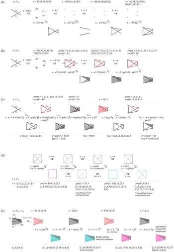
Figure 4 shows how allowing spatial and mechanical ambiguity could rapidly extend the design topology in early stages. The initial shape is recognized as two lines in algebra U 1j, and the boundary schema x → b(x) turns it into points (Fig. 4a, b). Perceptual iteration begins by applying schema x → x and x → prt(x) to recognize the points in a different order {e.g. (p 1, p 2, p 3, p 4) or [(p 3, p 1) (p 4, p 2)]}, and then the inverse boundary schema x → b −1(x) is applied based on this order (Fig. 4a–c). As a result, the schema not only returns the initial shape from the points but also yields other linear and planar compositions in the higher dimensions (see an alternating example of seeing and doing in Knight & Stiny, Reference Knight and Stiny2015). Ambiguity continues to catalyze design variations when registering the physical description. With a different visual attention to the part of shapes, applying different stiffness with schema E ← E[1(x)] or E ← E[0(x)] leads to different structural configurations (Fig. 4d, e).
(a–c): Recognition and boundary schema allows for different ways of perceiving the shape, which results in various configurations when followed by the inverse-boundary schema. (d, e) Recognition schema followed by Descriptive schema on applying the material property generates different structural configuration.

Case study
In the following case study, we demonstrate perceptual iteration and discuss its extended features, such as function, inverse-function, and recursion.
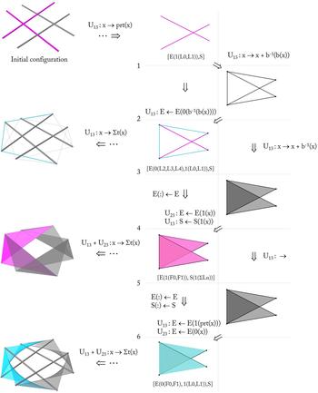
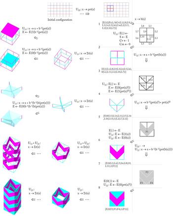
Figure 5 shows how perceptual iteration generates different structural topologies by changing the shape's description and the shape's algebra through reduction, recognition, and descriptive schemas. Consider the initial shape at the top of Figure 5 as two overlapping lines retrieved from a weaving configuration using the part schema. The description list (E, S) has an initial data {E[1(L0, L1)], S} which reads as “lines L0 and L1 are rigid.” Note that, in this example, we only show the properties that are modified, that is, material stiffness (E) and support's degree of freedom (S), and leave the other unmodified properties, L, A, and R, hidden.
Perceptual iteration on shifting one's perception on the traditional craft by alternating across different algebra with boundary and part schemas, and registering different physical description to the shape with descriptive schemas.

Through steps 1–3, the iteration is as follows: Schema x → x + b −1[b(x)] retrieves new lines from the existing line endpoints (L2, L3, L4). Schema E ← E[0(x)] registers a flexible material to the new lines and appends the description into {E[0(L2, L3, L4), 1(L0, L1)], S}. These three steps change the original configuration, where the two rigid lines are now tensioned by three new flexible lines. By applying schema x → Σt(x) to this module, we then have a new design that resembles a tensegrity structure.
The computation from steps 3 to 5 started with schema x → x + b −1(x) to retrieve two faces from existing line, thus x value for algebra U 23 is F0 and F1. Here, the previous material attributes are ignored with schema E(:) ← E empties the material data, thus returning it back to (E, S). The schema E ← E[1(x)] register rigid material to the faces, and schema S ← S[1(x)] turn all lines into a hinge which rotates around one axis. The list now consists of {E[1(F0, F1)], S[1(ΣLn)]}, which changes the tensegrity module into two faces connected with all lines as a hinge support. Applying x → Σt(x) to this module will return a folding configuration (see folding example in Jackson, Reference Jackson2011, and extended iteration in Muslimin, Reference Muslimin2016, Reference Muslimin2017)
Function schema
As the data and iterative steps in Figure 5 are explicit and recorded, the schema iteration can be compiled into functions to replicate the new topology for initial description: {E[1(ΣLn)], S}, and predicate: x is a set of interwoven lines in 3D space (x ∈ U 13). As listed below, function f 1(x) turns weaving into tensegrity and f 2(x) converts weaving into folding.

The double-arrow ⇒ in the function indicates a schema iteration, and the single arrow → designates a compiled schema. Note that the x value for the schema iteration in Figure 5, is the output from the last step. Hence the left-hand-variable is always reset to x. Inside the function, however, the variable's notation [e.g. b(x) or prt(x)] are preserved and nested in the subsequent steps to express how the visual calculation is progressing from the predicate. A new variable is introduced when the last output in the iteration is considered as a new shape (y).
As variables inside the function are modifiable, these functions serve as an open source to develop other possible topologies for inventive use. For instance, if hinges in f 2(x) are substituted into a fixed joint, S[0(y′ + y″)] instead of S[1(y′ + y″)], the function will produce a rigid folded-plate structure (Engel, Reference Engel1968; Weinand, Reference Weinand2009). Alternatively, instead of applying the rigid material to the faces in f 2(x), we can apply a flexible material to the faces using E ← E{0[b −1(y′ + y″)]}. As seen in the output in step 6, with the same rule schema iteration, this tweak creates a new function f 3(x), to develop a textile-tensegrity configuration from weaving (Peña Villamil et al., Reference Peña Villamil, Llorens Duran, Sastre Sastre, Crespo Artiaga and Tristancho Martínez2011).

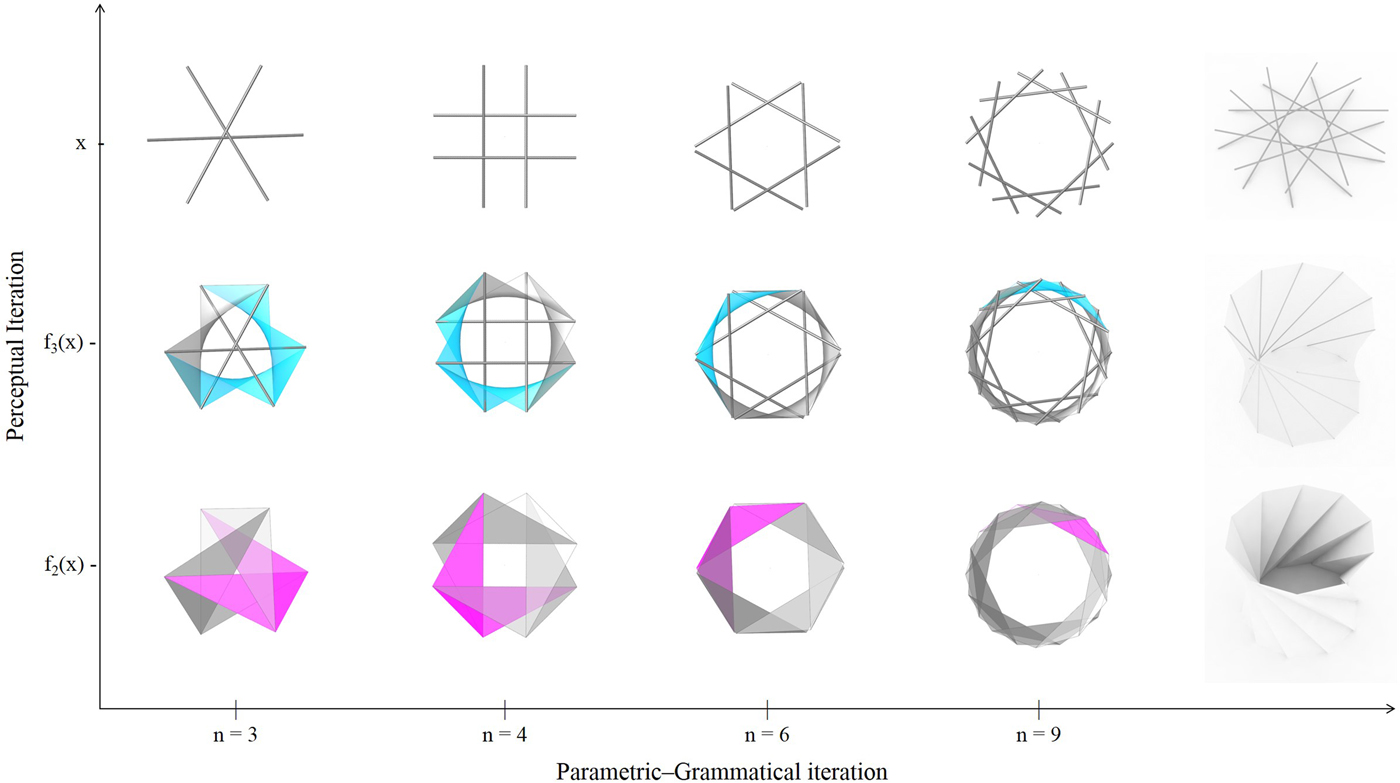
To convert rule schema into a shape rule, Stiny (Reference Stiny2006) shows how assignment g(x) → g[t(x)] turns rule schema x → t(x) into shape rule a → b (Stiny, Reference Stiny2006; Economou & Kotsopoulos, Reference Economou, Kotsopoulos, Gero and Hanna2015). In a similar manner, initial input from x, and outputs from f 2(x) and f 3(x) can be abbreviated into a shape rule: a → b + c, with function assignment, x → f n(x) and predicate: a is the overlapping composition of n lines (weaving), b is the rigid surface based on a’s inversed boundaries (folding), and c is a combination between the flexible surface from on a’s inversed boundaries and a’s lines’ composition (textile-tensegrity). This shape rule format is more practical and straightforward for quick application. The examples in Figure 6 show parametric-grammatical rule iterations along with perceptual iteration, where the modification in weaving (a) simultaneously alters the iteration in folding (b), and textile-tensegrity (c).
The iteration of Weaving-Tensegrity-Folding Function. Modification on one craft affects another type of craft's simultaneously.

Inversed function
With inverse schema A → B and B → A, the schema iteration within a function can be reversed to develop yet more functions. For example, function f 4(x) below converts tensegrity to folding from steps 3 to 5 in Figure 5. The initial description is: {E[0(L2, L3, L4)], 1(L0, L1), S}.

The steps of retrieving a face from a line in f 4(x) can be inversed from x ⇒ x + b −1(x) into x ⇒ b(x). As a result, we have a new function f 5(x) to convert the folding module into a tensegrity module. Figure 7 demonstrates this new function by using the Miura fold as the initial sample (Miura, Reference Miura1985; Muslimin, Reference Muslimin2016). A typical folding input is annotated with mountain creases (C M) and valley creases (C V), which indicates a series of hinge support (S) between faces on a 2D paper, such that {S[C v(prt(x)I), C m(prt(x)II)]}; x ∈ U 12. Steps 1–2 show the steps in producing a new structural configuration where all valley creases become flexible line (e.g. cables) and all mountain creases become rigid line (e.g. bars). The descriptive function converts the creases into either rigid or flexible lines, which change the description in Figure 7 from:
 $$\eqalign{& [E(1(\Sigma F_n ))\comma \,S(C_{\rm v} (L1\comma \,L8\comma \,L9\comma \,L3\comma \,L4\comma \,L5\comma \,L6)\comma C_{\rm m} (L2\comma \,L11\comma \,L12\comma \,L10\comma \,L7))] \cr & \quad \hbox{into}\; [E(1(L1\comma \,L8\comma \,L9\comma \,L3\comma \,L4\comma \,L5\comma \,L6)\comma \,0(L2\comma \,L11\comma \,L12\comma \,L10\comma \,L7))].} $$
Recursive schema
The schemas can continue to be applied in the subsequent steps in order to generate more structural topologies. Starting from step 2 in Figure 7, the iteration shows the boundary schema recursively applied to the new tensegrity modules. Applying the schema x → x + b −1{b[prt(x)]} returns new diagonal lines from the lines’ endpoints, and then, in step 4, another schema x → b −1[prt(x)I] + prt(x)II returns new faces (the arrowheads). For each new shapes from steps 3 and 5, descriptive schema E ← E[D E(x)] alternates between registering rigid and flexible material to derive new structural modules.
Perceptual-iteration process from Miura Folding crease to its Tensegrity version. Miura modules were recursively applied with reduction and descriptive schema to develop new tensegrity modules (right). Transformation schema is applied to generate 3D structures from these modules (left).

Transformation schema x → Σt(x) multiplies the 2D modules into 3D modules, from which inverse boundary schema b −1(x) can be reapplied to different parts of shape to create yet more new modules. The result is a series of space structures with a combination of rigid and flexible material that could respond to certain architectural requirements, such as enclosure (see left images in Fig. 7).
Structural simulation and physical validation
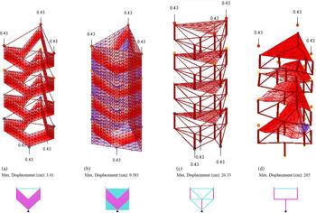
Figure 8 shows FEM analysis of four models from the above iteration. The transformation schema x → Σt(x) applied to the four models is the same. The models were rotated within a triangular base and stacked vertically four times. All four models have three fixed supporting points at the base, and three vertical loading points at the top with the same magnitude. While the stiffness of the cable, rigid bar, rigid surface and flexible membrane are the same across the four models, the main difference is in the mechanical configuration at the modular level.
• Model A has vertical rigid surfaces, supported by flexible cables.
• Model B has vertical rigid surfaces, supported by flexible membranes.
• Model C has horizontal flexible membranes which support trusses of rigid and flexible bar (thick bars are rigid).
• Model D has horizontal flexible membranes attached to the vertical rigid bar.
Finite Element Analysis on assessing several design results. All models have a triangular footprint and receive the same external load. Model A (rigid wall with cable) and B (rigid wall with fabric) are stable while model C and D collapsed.

All models were generated digitally, without initially considering their structural consequences. This leads to some peculiar model outputs, for example, the condition where the rigid surfaces in model B are supported only by flexible membranes that look structurally implausible. However, FEM analysis shows an opposite result. Out of the four, model B appears to have the smallest displacement of all (0.381 cm out of the total height 3 m) and model A has a larger displacement (3.41 cm), while model C and D have a very large displacement, and thus collapse.
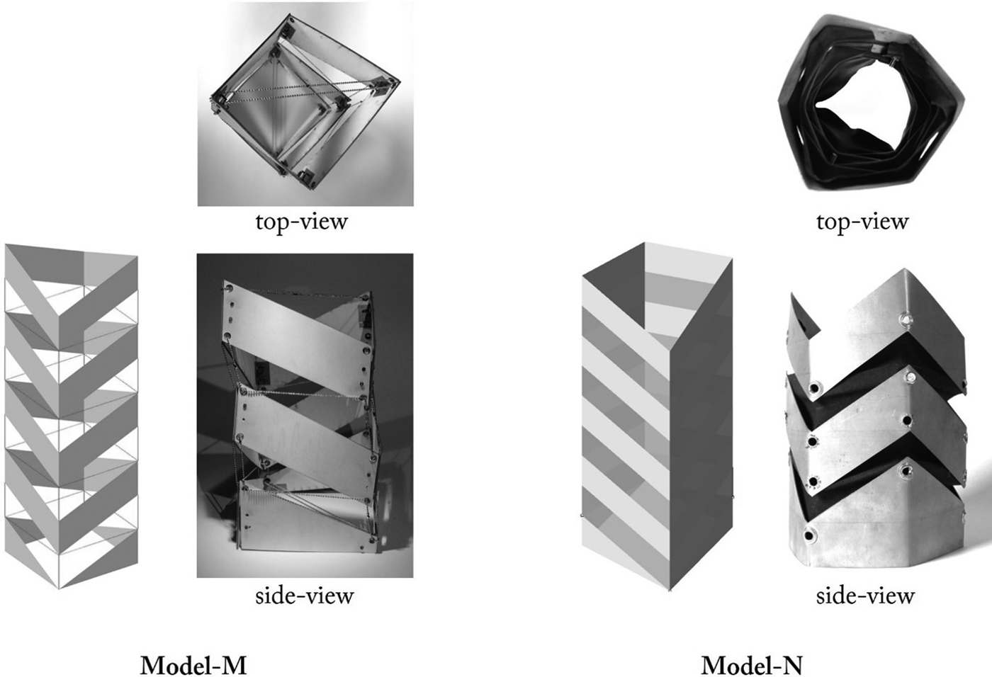
To validate these results, physical models (models M and N) were built to represent the configurations for models A and B (Fig. 9). The transformation schema is the same, except that the modules were stacked three times instead of four times, and the base for model M is square and model N is a hexagon. Therefore, these physical models have more supporting points and are shorter than their virtual versions.
Examples of physical validation from Miura Folding to Tensegrity iteration. Model M is based on model A consisted of a series of the rigid panel supported by chains (left), while in model N based on model B, the rigid panels are supported by black fabric (right).

The physical validation shows that, although model M and N may look rather unusual, they are physically stable. The rigid surfaces in model M are attached with aluminum ball-chains, while the rigid surfaces in model N are attached with black fabrics. As the chain has small strains and the fabric has large strains, model N’s fabric is stretched slightly downwards due to its own surface weight, yet it continues to support the surfaces well.
Conclusion
In this paper, we have illustrated and discussed different structural representation mechanisms using shape-grammar rule schemas. The schemas’ versatility for analyzing existing methods, as well as synthesizing a new method, is threefold:
First, the rule schema explicitly represents procedures underlying the structural method and interprets users’ perceptions through representing their design intentions. The schema representation indicates that an inclination toward a certain structural topology might be contributed by the modeling principles applied during the iteration process, that is, parametric and grammatical modeling. In parametric iterations, such as classical FEM and graphic statics, the design is optimized incrementally to achieve the equilibrium state while maintaining the shape's topology and the mechanical description. Grammatical iteration, on the other hand, alters the topologies using a set of generative rules. The rules might preserve a certain design language, as shown in the shape annealing method, or promote random designs, as seen in grammar-based graphic statics. Nevertheless, both methods work under predefined constraints, where parametric iteration constrains the shape relationship, grammatical iteration constrains the physical description.
Second, the rule schemas analysis suggests opportunities for new approaches in structural representation by highlighting some underutilized schemas. While the schemas in parametric and grammatical iterations mostly attached to physical description and operating in constant algebra, perceptual iteration loosened this attachment to foreground the role of user perception and ambiguity in deriving new structural configurations. Perceptual iteration constantly challenges the user to reconsider which shape to see and what to do with it, structurally or spatially. As a result, the iteration rapidly produces outputs beyond the initial topology. In addition, the schema iterations were able to produce a new set of functions that could be repeated or modified to synthesize a new topology.
Finally, this method allowed us to study the ideation process of the existing structural typology. In the example of converting weaving into tensegrity, the iteration provided ways to interpret the creative moment when the inventor, Kenneth Snelson, discovered tensegrity from weaving. It also revealed how such an ideation process might link to other crafting techniques, such as folding, thus paving a new path across disciplinary boundaries to enrich the language of structural design.
Acknowledgment
The author would like to thank the reviewers for their valuable feedback, George Stiny for his inputs on the schemas, and Cristina Ramos for analyzing model A to D.
Rizal Muslimin teaches at the University of Sydney. He holds a Ph.D. in Architecture: Design and Computation from Massachusetts Institute of Technology, United States. His computational design research centers at the intersection of craft, culture, and architecture. Dr. Muslimin has published scholarly articles in the field of computational craft, shape studies, and ethnocomputation in peer-reviewed journals and conferences. His research on computational craft had received best paper award and design awards.