1 Introduction
Our starting point is a quantitative version of Helly’s theorem on convex sets in Euclidean space. Helly’s theorem states that, if
 ${\mathcal{P}}=\{P_{i}:i\in I\}$
is a finite family of at least
 $n+1$
convex sets in
 $\mathbb{R}^{n}$
and if every
 $n+1$
or fewer members of
 ${\mathcal{P}}$
have non-empty intersection, then
 $\bigcap _{i\in I}P_{i}\neq \emptyset$
. This classical result and its variants have found important applications in discrete and computational geometry (see e.g. [Reference Danzer, Grünbaum and Klee14], [Reference Eckhoff17] and [Reference Amenta, De Loera and Soberón1]). Bárány et al proved in [Reference Bárány, Katchalski and Pach6] (see also [Reference Bárány, Katchalski and Pach7]) the following quantitative “volume version”.
Let
 ${\mathcal{P}}$
be a finite family of convex sets in
 $\mathbb{R}^{n}$
. If the intersection of every
 $2n$
or fewer members of
 ${\mathcal{P}}$
has volume greater than or equal to
 $1$
, then
 $\operatorname{vol}_{n}(\cap {\mathcal{P}})\geqslant c_{n}$
, where
 $c_{n}>0$
is a constant depending only on
 $n$
.
Throughout this article we write
 $\operatorname{vol}_{n}$
for the
 $n$
-dimensional Lebesgue measure (volume) of a convex set in
 $\mathbb{R}^{n}$
. Using the fact that every closed convex set is the intersection of a family of closed half-spaces and a simple compactness argument (see [Reference Bárány, Katchalski and Pach6]), one can remove the restriction that
 ${\mathcal{P}}$
is finite, provided that
 $\cap {\mathcal{P}}$
has positive volume, and also assume that each
 $P_{i}$
is a closed half-space. Therefore, the theorem of Bárány et al is equivalently stated as follows.
Let
 ${\mathcal{P}}$
be a family of closed half-spaces in
 $\mathbb{R}^{n}$
such that
 $\cap {\mathcal{P}}$
has positive volume. There exist
 $s\leqslant 2n$
and
 $i_{1},\ldots ,i_{s}\in I$
such that
 $$\begin{eqnarray}\operatorname{vol}_{n}(P_{i_{1}}\cap \cdots \cap P_{i_{s}})\leqslant C_{n}\operatorname{vol}_{n}(\cap {\mathcal{P}}),\end{eqnarray}$$
where
 $C_{n}>0$
is a constant depending only on
 $n$
.
Note that the cube
 $[-1,1]^{n}$
in
 $\mathbb{R}^{n}$
can be written as the intersection of the
 $2n$
closed half-spaces
 $H_{j}^{\pm }:=\{x:\langle x,\pm e_{j}\rangle \leqslant 1\}$
and that the intersection of any
 $2n-1$
of these half-spaces has infinite volume; this shows that one cannot replace
 $2n$
by
 $2n-1$
in the statement above. In [Reference Bárány, Katchalski and Pach6], the authors offered the bound
 $C_{n}\leqslant n^{2n^{2}}$
for the constant
 $C_{n}$
and they conjectured that one might actually have
 $C_{n}\leqslant n^{cn}$
for an absolute constant
 $c>0$
. Naszódi [Reference Naszódi26] has recently verified this conjecture; namely, he proved a volume version of Helly’s theorem with
 $C_{n}\leqslant (Cn)^{2n}$
, where
 $C>0$
is an absolute constant. Moreover, he gave an example which shows that one cannot hope for a bound better than
 $C_{n}\leqslant (Cn)^{n/2}$
in this statement. In §3, we present a slight modification of Naszódi’s argument, which leads to the exponent
 $3n/2$
instead of
 $2n$
.
Theorem 1.1. Let
 ${\mathcal{P}}=\{P_{i}:i\in I\}$
be a family of closed half-spaces such that
 $\cap {\mathcal{P}}$
has positive volume. We may find
 $s\leqslant 2n$
and
 $i_{1},\ldots ,i_{s}\in I$
such that
 $$\begin{eqnarray}\operatorname{vol}_{n}(P_{i_{1}}\cap \cdots \cap P_{i_{s}})\leqslant (Cn)^{3n/2}\operatorname{vol}_{n}(\cap {\mathcal{P}}),\end{eqnarray}$$
where
 $C>0$
is an absolute constant.
The aim of this work is to study a natural question that arises from Theorem 1.1. Given
 $N>2n$
, but proportional to
 $n$
, we would like to estimate the quantity
 $$\begin{eqnarray}C_{n,N}=\sup _{{\mathcal{P}}=\{P_{i}:i\in I\}}\,\inf \biggl\{\frac{\operatorname{vol}_{n}(P_{i_{1}}\cap \cdots \cap P_{i_{N}})}{\operatorname{vol}_{n}(\cap {\mathcal{P}})}:i_{1},\ldots ,i_{N}\in I\biggr\},\end{eqnarray}$$
where the supremum is taken over all families
 ${\mathcal{P}}=\{P_{i}:i\in I\}$
of closed half-spaces for which
 $\cap {\mathcal{P}}$
has finite and positive volume. A closely related, but not equivalent, question is to give an upper bound for the volume of the smallest polytope
 $P$
with
 $N$
facets that contains a given convex set of volume
 $1$
(for the rich literature in this area, the reader may consult the surveys of Gruber [Reference Gruber23] and Bronstein [Reference Bronstein12]).
Our first result concerns the case of families of symmetric strips in
 $\mathbb{R}^{n}$
. The proof of the next theorem presents the method that we would like to use in the general case and, because of the symmetry assumption, it is much simpler and leads to better bounds.
Theorem 1.2. Let
 ${\mathcal{P}}=\{P_{i}:i\in I\}$
be a family of symmetric strips
 $$\begin{eqnarray}P_{i}=\{x\in \mathbb{R}^{n}:|\langle x,u_{i}\rangle |\leqslant 1\}\end{eqnarray}$$
in
 $\mathbb{R}^{n}$
such that
 $\cap {\mathcal{P}}$
has positive volume. For every
 $d>1$
, there exist
 $s\leqslant dn$
and
 $i_{1},\ldots ,i_{s}\in I$
such that
 $$\begin{eqnarray}\operatorname{vol}_{n}(P_{i_{1}}\cap \cdots \cap P_{i_{s}})\leqslant \biggl(\frac{4\unicode[STIX]{x1D6FE}_{d}}{\unicode[STIX]{x1D70B}}\biggr)^{n/2}\unicode[STIX]{x1D6E4}\biggl(\frac{n}{2}+1\biggr)\operatorname{vol}_{n}(P),\end{eqnarray}$$
where
 $\unicode[STIX]{x1D6FE}_{d}:=((\sqrt{d}+1)/(\sqrt{d}-1))^{2}$
.
Note that if
 $d$
is not too close to
 $1$
, then the constant
 $C_{n,\lfloor dn\rfloor }$
is bounded by
 $(Cn)^{n/2}$
; the exponent
 $n/2$
is optimal (see Remark 6.1). In the non-symmetric case we can use a similar strategy (whose details are of course more delicate) to obtain an estimate comparable to the one in Theorem 1.1.
Theorem 1.3. Let
 ${\mathcal{P}}=\{P_{i}:i\in I\}$
be a family of closed half-spaces in
 $\mathbb{R}^{n}$
such that
 $\cap {\mathcal{P}}$
has positive volume. For every
 $d>1$
, there exist
 $s\leqslant (d+1)(n+1)$
and
 $i_{1},\ldots ,i_{s}\in I$
such that
 $$\begin{eqnarray}\displaystyle \operatorname{vol}_{n}(P_{i_{1}}\cap \cdots \cap P_{i_{s}}) & {\leqslant} & \displaystyle \unicode[STIX]{x1D6FE}_{d}^{(n+1)/2}\frac{n^{n/2}(n+1)^{3(n+1)/2}}{\unicode[STIX]{x1D70B}^{n/2}n!}\unicode[STIX]{x1D6E4}\biggl(\frac{n}{2}+1\biggr)\operatorname{vol}_{n}(\cap {\mathcal{P}})\nonumber\\ \displaystyle & {\leqslant} & \displaystyle (C_{d}n)^{3n/2}\operatorname{vol}_{n}(\cap {\mathcal{P}}),\end{eqnarray}$$
where
 $C_{d}=(e\unicode[STIX]{x1D6FE}_{d}/2\unicode[STIX]{x1D70B})^{1/3}$
.
Compared to Theorem 1.1, this theorem offers a better value of the constant
 $C_{d}$
when
 $d$
is large enough. If we further relax the condition on the number
 $s$
of half-spaces that we use, but still require that it is proportional to the dimension, we are able to prove the following improved bound.
Theorem 1.4. There exists an absolute constant
 $\unicode[STIX]{x1D6FC}>1$
with the following property: for every family
 ${\mathcal{P}}=\{P_{i}:i\in I\}$
of closed half-spaces in
 $\mathbb{R}^{n}$
such that
 $\cap {\mathcal{P}}$
has positive volume, there exist
 $s\leqslant \unicode[STIX]{x1D6FC}n$
and
 $i_{1},\ldots ,i_{s}\in I$
such that
 $$\begin{eqnarray}\operatorname{vol}_{n}(P_{i_{1}}\cap \cdots \cap P_{i_{s}})\leqslant (Cn)^{n}\operatorname{vol}_{n}(\cap {\mathcal{P}}),\end{eqnarray}$$
where
 $C>0$
is an absolute constant.
Let us note that, in the recent paper [Reference De Loera, La Haye, Rolnick and Soberón15], De Loera et al have presented many interesting results, both continuous and discrete, that may be viewed as quantitative versions of Carathéodory’s, Helly’s and Tverberg’s theorems. For example, they proved that for every
 $n\geqslant 1$
and
 $\unicode[STIX]{x1D700}>0$
there exists a positive integer
 $N=N(n,\unicode[STIX]{x1D700})$
with the following property: if
 ${\mathcal{F}}=\{F_{i}:i\in I\}$
is a finite family of convex sets in
 $\mathbb{R}^{n}$
such that
 $\operatorname{vol}_{n}(F_{i_{1}}\cap \cdots \cap F_{i_{s}})\geqslant 1$
for all
 $s\leqslant Nn$
and all
 $i_{1},\ldots ,i_{s}\in I$
, then
 $$\begin{eqnarray}\operatorname{vol}_{n}(\cap {\mathcal{F}})\geqslant \frac{1}{1+\unicode[STIX]{x1D700}}.\end{eqnarray}$$
They also obtained a variant of this statement in which volume is replaced by diameter, as well as a “colorful” volume version of Helly’s theorem. The parameter
 $N(n,\unicode[STIX]{x1D700})$
is defined as the smallest integer such that, for every convex set
 $K\subset \mathbb{R}^{n}$
of positive volume, there exists a polytope
 $P\supseteq K$
with at most
 $N(n,\unicode[STIX]{x1D700})$
facets such that
 $\operatorname{vol}_{n}(P)\leqslant (1+\unicode[STIX]{x1D700})\operatorname{vol}_{n}(K)$
, and it is known that
 $N(n,\unicode[STIX]{x1D700})$
is exponential in
 $n$
and
 $\unicode[STIX]{x1D700}$
: in [Reference Gordon, Meyer and Reisner21] and [Reference Gordon, Reisner and Schütt22], it is proved that
 $$\begin{eqnarray}\biggl(\frac{c_{1}n}{\unicode[STIX]{x1D700}}\biggr)^{(n-1)/2}\leqslant N(n,\unicode[STIX]{x1D700})\leqslant \biggl(\frac{c_{2}n}{\unicode[STIX]{x1D700}}\biggr)^{(n-1)/2}.\end{eqnarray}$$
We emphasize that the philosophy of all these results is completely different from the one in our work. We are interested in the best lower bound that one can get for
 $\operatorname{vol}_{n}(\cap {\mathcal{F}})$
starting from a lower bound for the volume of the intersections of subfamilies that have small cardinality, i.e. proportional to the dimension.
We close this introductory section by briefly explaining the main ideas behind the proof of our results. We may assume that
 $\cap {\mathcal{P}}=\bigcap _{i\in I}\{x\in \mathbb{R}^{n}:\langle x,u_{i}\rangle \leqslant 1\}$
has finite volume and, since the statements are affinely invariant, that
 $\cap {\mathcal{P}}$
is in John’s position, i.e. the ellipsoid of maximal volume inscribed in
 $\cap {\mathcal{P}}$
is the Euclidean unit ball
 $B_{2}^{n}$
. Then we have John’s decomposition of the identity (see §2 for background information): there exists
 $J\subseteq I$
such that
 $u_{j}$
,
 $j\in J$
, are contact points of
 $\cap {\mathcal{P}}$
and
 $B_{2}^{n}$
and there are positive scalars
 $a_{j}$
,
 $j\in J$
, such that
 $$\begin{eqnarray}I_{n}=\mathop{\sum }_{j\in J}a_{j}u_{j}\otimes u_{j}\qquad \text{and}\qquad \mathop{\sum }_{j\in J}a_{j}u_{j}=0.\end{eqnarray}$$
Then we would like to exploit an appropriate variant of Ball’s proof of the reverse isoperimetric inequality in [Reference Ball4] in order to estimate the volume of
 $Q:=\bigcap _{j\in J}P_{j}$
. For example, in order to prove Theorem 1.2, we would write
 $$\begin{eqnarray}\operatorname{vol}_{n}(Q)=\int _{\mathbb{R}^{n}}\mathop{\prod }_{j\in J}f_{j}^{a_{j}}(\langle x,u_{j}\rangle )\,dx,\end{eqnarray}$$
where
 $f_{j}(t)=\mathbf{1}_{[-1,1]}(t)$
, and then use the geometric Brascamp–Lieb inequality
 $$\begin{eqnarray}\int _{\mathbb{R}^{n}}\mathop{\prod }_{j\in J}f_{j}^{a_{j}}(\langle x,u_{j}\rangle )\,dx\leqslant \mathop{\prod }_{j\in J}\biggl(\int _{\mathbb{R}}f_{j}(t)\,dt\biggr)^{a_{j}}\end{eqnarray}$$
(see §5) to bound the integral on the right-hand side of (1.11). For the non-symmetric case one usually exploits an idea of Ball to obtain an integral representation of
 $\operatorname{vol}_{n}(Q)$
for which (1.12) can be applied; see (6.40). The problem is that by John’s theorem the cardinality of the set
 $J$
is of the order of
 $n^{2}$
in general, while we need to find a subfamily of the
 $P_{j}$
of cardinality proportional to
 $n$
. To this end, given
 $d>1$
, we would like to extract a subset
 $\unicode[STIX]{x1D70E}$
of
 $J$
, of cardinality
 $\lfloor dn\rfloor$
, which still forms an approximate John’s decomposition of the identity with suitable weights (this idea has been used in [Reference Gluskin and Litvak20] and [Reference Barvinok8]). One such result is the following theorem of Batson et al from [Reference Batson, Spielman and Srivastava9]: there exists a subset
 $\unicode[STIX]{x1D70E}\subseteq J$
with
 $|\unicode[STIX]{x1D70E}|\leqslant dn$
and
 $c_{j}>0$
,
 $j\in \unicode[STIX]{x1D70E}$
, such that
 $$\begin{eqnarray}I_{n}\preccurlyeq \mathop{\sum }_{j\in \unicode[STIX]{x1D70E}}c_{j}u_{j}\otimes u_{j}\preccurlyeq \unicode[STIX]{x1D6FE}_{d}I_{n},\end{eqnarray}$$
where
 $\unicode[STIX]{x1D6FE}_{d}:=((\sqrt{d}+1)/(\sqrt{d}-1))^{2}$
. This fact is used for the proof of Theorems 1.2 and 1.3. For the proof of Theorem 1.4, we use a second, more delicate, theorem of Srivastava from [Reference Srivastava30] (see §4 for the precise statement).
The main problem now is to obtain an analogue of (1.12), when, instead of (1.10), we only have the approximate John’s decomposition (1.13). To the best of our knowledge this question had not been studied. Our main technical result, which resolves this problem, is the next theorem; we feel that it is a useful tool of independent interest.
Theorem 1.5. Let
 $\unicode[STIX]{x1D6FE}>1$
. Let
 $u_{1},\ldots ,u_{s}\in S^{n-1}$
and
 $c_{1},\ldots ,c_{s}>0$
satisfy
 $$\begin{eqnarray}I_{n}\preccurlyeq A:=\mathop{\sum }_{j=1}^{s}c_{j}u_{j}\otimes u_{j}\preccurlyeq \unicode[STIX]{x1D6FE}I_{n}\end{eqnarray}$$
and set
 $\unicode[STIX]{x1D705}_{j}=c_{j}\langle A^{-1}u_{j},u_{j}\rangle >0$
,
 $1\leqslant j\leqslant s$
. Then
 $\sum _{j=1}^{s}k_{j}=n$
and, if
 $f_{1},\ldots ,f_{s}:\mathbb{R}\rightarrow \mathbb{R}^{+}$
are integrable functions, we have
 $$\begin{eqnarray}\int _{\mathbb{R}^{n}}\mathop{\prod }_{j=1}^{s}f_{j}^{\unicode[STIX]{x1D705}_{j}}(\langle x,u_{j}\rangle )\,dx\leqslant \unicode[STIX]{x1D6FE}^{n/2}\mathop{\prod }_{j=1}^{s}\biggl(\int _{\mathbb{ R}}f_{j}(t)\,dt\biggr)^{\unicode[STIX]{x1D705}_{j}}.\end{eqnarray}$$
In §6, we present the proofs of the main results.
2 Notation and background
We work in
 $\mathbb{R}^{n}$
, which is equipped with a Euclidean structure
 $\langle \cdot ,\cdot \rangle$
. We denote by
 $\Vert \cdot \Vert _{2}$
the corresponding Euclidean norm, and write
 $B_{2}^{n}$
for the Euclidean unit ball and
 $S^{n-1}$
for the unit sphere. The volume (Lebesgue measure) of a convex set
 $A\subset \mathbb{R}^{n}$
is denoted by
 $\text{vol}_{n}(A)$
. We write
 $\unicode[STIX]{x1D714}_{n}$
for the volume of
 $B_{2}^{n}$
and
 $\unicode[STIX]{x1D70E}$
for the rotationally invariant probability measure on
 $S^{n-1}$
. Recall that
 $$\begin{eqnarray}\unicode[STIX]{x1D714}_{n}=\operatorname{vol}_{n}(B_{2}^{n})=\frac{\unicode[STIX]{x1D70B}^{n/2}}{\unicode[STIX]{x1D6E4}(n/2+1)}.\end{eqnarray}$$
The letters
 $c,c^{\prime },c_{1},c_{2}$
etc denote absolute positive constants, which may change from line to line.
We refer to the book of Schneider [Reference Schneider29] for basic facts from Brunn–Minkowski theory and to the book of Artstein-Avidan et al [Reference Artstein-Avidan, Giannopoulos and Milman2] for basic facts from asymptotic convex geometry.
A convex body in
 $\mathbb{R}^{n}$
is a compact convex subset
 $K$
of
 $\mathbb{R}^{n}$
with non-empty interior. We say that
 $K$
is symmetric if
 $x\in K$
implies that
 $-x\in K$
, and that
 $K$
is centered if its barycenter
 $$\begin{eqnarray}\text{bar}(K)=\frac{1}{\operatorname{vol}_{n}(K)}\int _{K}x\,dx\end{eqnarray}$$
is at the origin. The polar body
 $K^{\circ }$
of
 $K$
is defined by
 $$\begin{eqnarray}K^{\circ }:=\{y\in \mathbb{R}^{n}:\langle x,y\rangle \leqslant 1\text{ for all }x\in K\}.\end{eqnarray}$$
The Blaschke–Santaló inequality (see [Reference Artstein-Avidan, Giannopoulos and Milman2, Theorem 1.5.10]) states that for every centered convex body
 $K$
in
 $\mathbb{R}^{n}$
, one has
 $\operatorname{vol}_{n}(K)\operatorname{vol}_{n}(K^{\circ })\leqslant \unicode[STIX]{x1D714}_{n}^{2}$
, with equality if and only if
 $K$
is an ellipsoid. The reverse Santaló inequality of Bourgain and Milman [Reference Bourgain and Milman10] states that there exists an absolute constant
 $c>0$
such that
 $$\begin{eqnarray}(\operatorname{vol}_{n}(K)\operatorname{vol}_{n}(K^{\circ }))^{1/n}\geqslant c/n\end{eqnarray}$$
for every convex body
 $K$
in
 $\mathbb{R}^{n}$
which contains
 $0$
in its interior.
We say that a convex body
 $K$
is in John’s position if the ellipsoid of maximal volume inscribed in
 $K$
is the Euclidean unit ball
 $B_{2}^{n}$
. John’s theorem [Reference John24] states that
 $K$
is in John’s position if and only if
 $B_{2}^{n}\subseteq K$
and there exist
 $u_{1},\ldots ,u_{m}\in \text{bd}(K)\cap S^{n-1}$
(contact points of
 $K$
and
 $B_{2}^{n}$
) and positive real numbers
 $c_{1},\ldots ,c_{m}$
such that
 $$\begin{eqnarray}\mathop{\sum }_{j=1}^{m}c_{j}u_{j}=0\end{eqnarray}$$
and the identity operator
 $I_{n}$
is decomposed in the form
 $$\begin{eqnarray}I_{n}=\mathop{\sum }_{j=1}^{m}c_{j}u_{j}\otimes u_{j},\end{eqnarray}$$
where
 $(u_{j}\otimes u_{j})(y)=\langle u_{j},y\rangle u_{j}$
. In the case where
 $K$
is symmetric, the second condition (2.5) is enough (for any contact point
 $u$
, we have that
 $-u$
is also a contact point and, hence, having (2.5), we may easily produce a decomposition for which (2.4) is also satisfied).
Assume that
 $u_{1},\ldots ,u_{m}$
are unit vectors that satisfy John’s decomposition (2.5) with some positive weights
 $c_{j}$
. Then one has the identities
 $$\begin{eqnarray}\mathop{\sum }_{j=1}^{m}c_{j}=\text{tr}(I_{n})=n\qquad \text{and}\qquad \mathop{\sum }_{j=1}^{m}c_{j}\langle u_{j},z\rangle ^{2}=1\end{eqnarray}$$
for all
 $z\in S^{n-1}$
. Moreover,
 $$\begin{eqnarray}\text{conv}\{u_{1},\ldots ,u_{m}\}\supseteq \frac{1}{n}B_{2}^{n}.\end{eqnarray}$$
In the symmetric case, we actually have
 $$\begin{eqnarray}\text{conv}\{\pm u_{1},\ldots ,\pm u_{m}\}\supseteq \frac{1}{\sqrt{n}}B_{2}^{n}.\end{eqnarray}$$
Another fact, which goes back to the classical article of Dvoretzky and Rogers [Reference Dvoretzky and Rogers16], is that we may choose
 $v_{1},\ldots ,v_{n}$
, among the
 $u_{i}$
, which satisfy
 $$\begin{eqnarray}\text{dist}(v_{k},\text{span}(v_{1},v_{2},\ldots ,v_{k-1}))\geqslant \sqrt{\frac{n-k+1}{n}}\end{eqnarray}$$
for all
 $k=2,\ldots ,n$
. This plays a key role in Naszódi’s argument; see the next section.
Finally, we state as a lemma a fact from linear algebra that will be used in §5.
Lemma 2.1. Let
 $A$
be an
 $n\times n$
invertible matrix. For any
 $u,v\in \mathbb{R}^{n}$
, we have
 $$\begin{eqnarray}\det (A+u\otimes v)=\det (A)(1+\langle A^{-1}u,v\rangle ).\end{eqnarray}$$
Proof. Let
 $u,v\in \mathbb{R}^{n}$
. Since
 $u\otimes v$
is a rank-one matrix with one non-zero eigenvalue equal to
 $\langle u,v\rangle$
, it is clear that
 $\det (I_{n}+u\otimes v)=1+\langle u,v\rangle$
, which is the assertion of the lemma in the case
 $A=I_{n}$
. Given any
 $n\times n$
invertible matrix
 $A$
, we write
 $$\begin{eqnarray}A+u\otimes v=A(I_{n}+A^{-1}(u\otimes v))=A(I_{n}+(A^{-1}u\otimes v))\end{eqnarray}$$
and, applying the previous special case, we obtain
 $$\begin{eqnarray}\det (A+u\otimes v)=\det (A)\det (I_{n}+(A^{-1}u\otimes v))=\det (A)(1+\langle A^{-1}u,v\rangle ),\end{eqnarray}$$
as claimed. ◻
3 A refinement of Naszódi’s argument
We start with a refinement of Naszódi’s argument from [Reference Naszódi26]; our only new ingredient is the fact that every convex body
 $K$
contains a centrally symmetric convex body
 $K_{1}$
of volume
 $\operatorname{vol}_{n}(K_{1})\geqslant 2^{-n}\operatorname{vol}_{n}(K)$
. Incorporating this in the original proof, we obtain a better estimate.
Proof of Theorem 1.1.
We start with a family
 ${\mathcal{P}}=\{P_{i}:i\in I\}$
of closed half-spaces
 $P_{i}=\{x:\langle x,u_{i}\rangle \leqslant 1\}$
such that
 $P:=\cap {\mathcal{P}}$
has positive and finite volume. We may assume that
 ${\mathcal{P}}$
is a finite family; therefore,
 $P$
is a polytope. By affine invariance, we may also assume that
 $P$
is in John’s position. From John’s theorem, there exists
 $J\subseteq I$
such that
 $u_{j}$
,
 $j\in J$
, are contact points of
 $P$
and
 $B_{2}^{n}$
, and
 $a_{j}>0$
,
 $j\in J$
, such that
 $$\begin{eqnarray}I_{n}=\mathop{\sum }_{j\in J}a_{j}u_{j}\otimes u_{j}\qquad \text{and}\qquad \mathop{\sum }_{j\in J}a_{j}u_{j}=0.\end{eqnarray}$$
By the Dvoretzky–Rogers lemma, we may choose
 $n$
of these contact points, which we denote by
 $v_{1},\ldots ,v_{n}$
, so that
 $$\begin{eqnarray}\text{dist}(v_{k},\text{span}(v_{1},v_{2},\ldots ,v_{k-1}))\geqslant \sqrt{\frac{n-k+1}{n}}\end{eqnarray}$$
for all
 $k=2,\ldots ,n$
. It follows that the simplex
 $S=\text{conv}\{v_{0}=0,v_{1},\ldots ,v_{n}\}\subseteq P$
has volume
 $$\begin{eqnarray}\operatorname{vol}_{n}(S)=\frac{1}{n!}\mathop{\prod }_{k=1}^{n}\text{dist}(v_{k},\text{span}(v_{1},v_{2},\ldots ,v_{k-1}))\geqslant \frac{1}{n^{n/2}\sqrt{n!}}.\end{eqnarray}$$
Now we use the fact (see [Reference Artstein-Avidan, Giannopoulos and Milman2, Theorem 4.1.20]) that if
 $w$
is the center of mass of
 $S$
, then
 $S-w$
contains an origin-symmetric convex body
 $T_{1}$
of volume
 $\operatorname{vol}_{n}(T_{1})\geqslant 2^{-n}\text{vol}_{n}(S-w)=2^{-n}\operatorname{vol}_{n}(S)$
and hence the convex body
 $T=T_{1}+w\subseteq S$
has a center of symmetry at
 $w$
and satisfies
 $$\begin{eqnarray}\operatorname{vol}_{n}(T)\geqslant 2^{-n}\text{vol}_{n}(S).\end{eqnarray}$$
Consider the ray
 $\ell$
from the origin in the direction of
 $-w$
. Then
 $\ell$
intersects the boundary of
 $\text{conv}\{u_{j},j\in J\}$
at a point
 $z\in \text{conv}\{v_{n+1},\ldots ,v_{n+k}\}$
for some
 $v_{n+i}\in \{u_{j},j\in J,\}$
and
 $k\leqslant n$
(this follows from Carathéodory’s theorem). Also, note that
 $\text{conv}\{u_{j},j\in J\}\supseteq (1/n)B_{2}^{n}$
and hence
 $\Vert z\Vert _{2}\geqslant 1/n$
. Applying a contraction with center
 $z$
and ratio
 $$\begin{eqnarray}\unicode[STIX]{x1D706}=\frac{\Vert z\Vert _{2}}{\Vert z-w\Vert _{2}}=\frac{\Vert z\Vert _{2}}{\Vert z\Vert _{2}+\Vert w\Vert _{2}}\geqslant \frac{\Vert z\Vert _{2}}{1+\Vert z\Vert _{2}}\geqslant \frac{1}{n+1}\end{eqnarray}$$
to
 $T$
, we obtain an origin-symmetric convex body
 $$\begin{eqnarray}Q\subseteq \text{conv}\{z,v_{1},\ldots ,v_{n}\}\subseteq \text{conv}\{v_{1},\ldots ,v_{n},v_{n+1},\ldots ,v_{n+k}\}\end{eqnarray}$$
with volume
 $$\begin{eqnarray}\displaystyle \operatorname{vol}_{n}(Q) & {\geqslant} & \displaystyle \frac{1}{(n+1)^{n}}\text{vol}_{n}(T)\geqslant \frac{1}{2^{n}(n+1)^{n}}\text{vol}_{n}(S)\nonumber\\ \displaystyle & {\geqslant} & \displaystyle \frac{1}{2^{n}(n+1)^{n}n^{n/2}\sqrt{n!}}.\end{eqnarray}$$
Consider the intersection of
 $n+k\leqslant 2n$
half-spaces
 $$\begin{eqnarray}R=\mathop{\bigcap }_{i=1}^{n+k}\{x\in \mathbb{R}^{n}:\langle x,v_{i}\rangle \leqslant 1\}.\end{eqnarray}$$
Using the Blaschke–Santaló inequality for
 $Q$
and the facts that
 $B_{2}^{n}\subseteq P$
and
 $R\subseteq Q^{\circ }$
, we get
 $$\begin{eqnarray}\frac{\operatorname{vol}_{n}(R)}{\text{vol}_{n}(P)}\leqslant \frac{\operatorname{vol}_{n}(Q^{\circ })}{\text{vol}_{n}(B_{2}^{n})}\leqslant \frac{\operatorname{vol}_{n}(B_{2}^{n})}{\text{vol}_{n}(Q)}.\end{eqnarray}$$
Finally, from (3.6), we see that
 $$\begin{eqnarray}\operatorname{vol}_{n}(R)\leqslant \frac{\unicode[STIX]{x1D70B}^{n/2}2^{n}(n+1)^{n}n^{n/2}\sqrt{n!}}{\unicode[STIX]{x1D6E4}((n/2)+1)}\operatorname{vol}_{n}(P),\end{eqnarray}$$
and the result follows (with constant
 $C=2\sqrt[3]{\unicode[STIX]{x1D70B}}$
, as one can check using Stirling’s formula).◻
4 Approximate John’s decompositions
Our first main tool is the work of Batson et al [Reference Batson, Spielman and Srivastava9] on spectral sparsification of graphs, in which they introduced a deterministic method extracting an approximate John’s decomposition starting from a John’s decomposition of the form (2.5). Their result is the following.
Theorem 4.1 (Batson et al).
Let
 $v_{1},\ldots ,v_{m}\in S^{n-1}$
and
 $a_{1},\ldots ,a_{m}>0$
be such that
 $$\begin{eqnarray}I_{n}=\mathop{\sum }_{j=1}^{m}a_{j}v_{j}\otimes v_{j}.\end{eqnarray}$$
Then, for every
 $d>1$
, there exists a subset
 $\unicode[STIX]{x1D70E}\subseteq \{1,\ldots ,m\}$
with
 $|\unicode[STIX]{x1D70E}|\leqslant dn$
and
 $b_{j}>0$
,
 $j\in \unicode[STIX]{x1D70E}$
, such that
 $$\begin{eqnarray}I_{n}\preccurlyeq \mathop{\sum }_{j\in \unicode[STIX]{x1D70E}}b_{j}a_{j}v_{j}\otimes v_{j}\preccurlyeq \unicode[STIX]{x1D6FE}_{d}I_{n},\end{eqnarray}$$
where
 $$\begin{eqnarray}\unicode[STIX]{x1D6FE}_{d}:=\biggl(\frac{\sqrt{d}+1}{\sqrt{d}-1}\biggr)^{2}.\end{eqnarray}$$
Here, given two symmetric positive-definite matrices
 $A$
and
 $B$
, we write
 $A\preccurlyeq B$
if
 $\langle Ax,x\rangle \leqslant \langle Bx,x\rangle$
for all
 $x\in \mathbb{R}^{n}$
. Using this fact, Srivastava [Reference Srivastava30] obtained an improved version of Rudelson’s theorem [Reference Rudelson28] on the approximation of a symmetric convex body
 $K$
by a symmetric convex body
 $T$
which has few contact points with its maximal volume ellipsoid: for any symmetric convex body
 $K$
in
 $\mathbb{R}^{n}$
and any
 $\unicode[STIX]{x1D700}>0$
, there exists a symmetric convex body
 $T$
such that
 $T\subseteq K\subseteq (1+\unicode[STIX]{x1D700})T$
and
 $T$
has at most
 $32n/\unicode[STIX]{x1D700}^{2}$
contact points with its John ellipsoid.
In order to deal with the non-symmetric case of this question, Srivastava proved in [Reference Srivastava30] the next variant of Theorem 4.1.
Theorem 4.2 (Srivastava).
Let
 $v_{1},\ldots ,v_{m}\in S^{n-1}$
and
 $a_{1},\ldots ,a_{m}>0$
be such that
 $$\begin{eqnarray}I_{n}=\mathop{\sum }_{j=1}^{m}a_{j}v_{j}\otimes v_{j}\qquad \text{and}\qquad \mathop{\sum }_{j=1}^{m}a_{j}v_{j}=0.\end{eqnarray}$$
Given
 $\unicode[STIX]{x1D700}>0$
, we can find a subset
 $\unicode[STIX]{x1D70E}$
of
 $\{1,\ldots ,m\}$
of cardinality
 $|\unicode[STIX]{x1D70E}|\leqslant Cn/\unicode[STIX]{x1D700}^{2}$
, positive scalars
 $c_{i}$
,
 $i\in \unicode[STIX]{x1D70E}$
, and a vector
 $v$
with
 $$\begin{eqnarray}\Vert v\Vert _{2}^{2}\leqslant \frac{\unicode[STIX]{x1D700}}{\mathop{\sum }_{i\in \unicode[STIX]{x1D70E}}c_{i}}\end{eqnarray}$$
such that
 $$\begin{eqnarray}I_{n}\preccurlyeq \mathop{\sum }_{i\in \unicode[STIX]{x1D70E}}c_{i}(v_{i}+v)\otimes (v_{i}+v)\preccurlyeq (4+\unicode[STIX]{x1D700})I_{n}\end{eqnarray}$$
and
 $$\begin{eqnarray}\mathop{\sum }_{i\in \unicode[STIX]{x1D70E}}c_{i}(v_{i}+v)=0.\end{eqnarray}$$
Using Theorem 4.2, Srivastava showed that for any convex body
 $K$
in
 $\mathbb{R}^{n}$
and any
 $\unicode[STIX]{x1D700}>0$
, there exists a convex body
 $T$
such that
 $T\subseteq K\subseteq (\sqrt{5}+\unicode[STIX]{x1D700})T$
and
 $T$
has at most
 $Cn/\unicode[STIX]{x1D700}^{2}$
contact points with its John ellipsoid. Friedland and Youssef (see [Reference Friedland and Youssef18]) have recently obtained optimal forms of Srivastava’s result in which the constant
 $4+\unicode[STIX]{x1D700}$
in (4.6) and the constant
 $\sqrt{5}+\unicode[STIX]{x1D700}$
above are replaced by
 $1+\unicode[STIX]{x1D700}$
. Their argument exploits the solution of the Kadison–Singer problem by Marcus et al (see [Reference Marcus, Spielman and Srivastava25]).
We will use Theorem 4.2 in order to deal with the non-symmetric case of our problem, which is clearly much more interesting than the symmetric one.
5 Brascamp–Lieb inequality and approximate John’s decompositions
The Brascamp–Lieb inequality [Reference Brascamp and Lieb11] estimates the norm of the multilinear operator
 $G:L^{p_{1}}(\mathbb{R})\times \cdots \times L^{p_{m}}(\mathbb{R})\rightarrow \mathbb{R}$
defined by
 $$\begin{eqnarray}G(f_{1},\ldots ,f_{m})=\int _{\mathbb{R}^{n}}\mathop{\prod }_{j=1}^{m}f_{j}(\langle x,u_{j}\rangle )\,dx,\end{eqnarray}$$
where
 $m\geqslant n$
,
 $p_{1},\ldots ,p_{m}\geqslant 1$
with
 $(1/p_{1})+\cdots +(1/p_{m})=n$
and
 $u_{1},\ldots ,u_{m}\in \mathbb{R}^{n}$
. Brascamp and Lieb proved that the norm of
 $G$
is the supremum
 $D$
of
 $$\begin{eqnarray}\frac{G(g_{1},\ldots ,g_{m})}{\mathop{\prod }_{j=1}^{m}\Vert g_{j}\Vert _{p_{j}}}\end{eqnarray}$$
over all centered Gaussian functions
 $g_{1},\ldots ,g_{m}$
, i.e. over all functions of the form
 $g_{j}(t)=\text{e}^{-\unicode[STIX]{x1D706}_{j}t^{2}}$
,
 $\unicode[STIX]{x1D706}_{j}>0$
.
If we set
 $c_{j}=1/p_{j}$
and replace
 $f_{j}$
by
 $f_{j}^{c_{j}}$
, then we can state the Brascamp–Lieb inequality in the following form.
Theorem 5.1 (Brascamp–Lieb).
Let
 $m\geqslant n$
, and let
 $u_{1},\ldots ,u_{m}\in \mathbb{R}^{n}$
and
 $c_{1},\ldots ,c_{m}>0$
with
 $c_{1}+\cdots +c_{m}=n$
. Then
 $$\begin{eqnarray}\int _{\mathbb{R}^{n}}\mathop{\prod }_{j=1}^{m}f_{j}^{c_{j}}(\langle x,u_{j}\rangle )\,dx\leqslant D\,\mathop{\prod }_{j=1}^{m}\biggl(\int _{\mathbb{ R}}f_{j}\biggr)^{c_{j}}\end{eqnarray}$$
for all integrable functions
 $f_{j}:\mathbb{R}\rightarrow [0,\infty )$
, where
 $D=1/\sqrt{F}$
and
 $$\begin{eqnarray}F=\inf \biggl\{\frac{\det (\mathop{\sum }_{j=1}^{m}c_{j}\unicode[STIX]{x1D706}_{j}u_{j}\otimes u_{j})}{\mathop{\prod }_{j=1}^{m}\unicode[STIX]{x1D706}_{j}^{c_{j}}}:\unicode[STIX]{x1D706}_{j}>0\biggr\}.\end{eqnarray}$$
Calculating the constant
 $F=F(\{u_{j}\},\{c_{j}\})$
in Theorem 5.1 seems difficult. An important observation of Ball (see e.g. [Reference Ball3]) is that if
 $u_{1},\ldots ,u_{m}\in S^{n-1}$
and
 $c_{1},\ldots ,c_{m}>0$
satisfy John’s decomposition of the identity (2.5), then the constant
 $F=F(\{u_{j}\},\{c_{j}\})$
in Theorem 5.1 is equal to
 $1$
.
The next proposition shows that we still have a Brascamp–Lieb inequality with a reasonable constant when an approximate John’s decomposition is available.
Proposition 5.2. Let
 $\unicode[STIX]{x1D6FE}>1$
. Assume that
 $u_{1},\ldots ,u_{s}\in S^{n-1}$
and
 $c_{1},\ldots ,c_{s}>0$
satisfy
 $$\begin{eqnarray}I_{n}\preccurlyeq A:=\mathop{\sum }_{j=1}^{s}c_{j}u_{j}\otimes u_{j}\preccurlyeq \unicode[STIX]{x1D6FE}I_{n}.\end{eqnarray}$$
Then, if we define
 $\unicode[STIX]{x1D705}_{j}=c_{j}\langle A^{-1}u_{j},u_{j}\rangle >0$
,
 $1\leqslant j\leqslant s$
, we have that
 $\sum _{j=1}^{s}\unicode[STIX]{x1D705}_{j}=n$
and
 $$\begin{eqnarray}\unicode[STIX]{x1D6FE}^{n}\det \biggl(\mathop{\sum }_{j=1}^{s}\unicode[STIX]{x1D705}_{j}\unicode[STIX]{x1D706}_{j}u_{j}\otimes u_{j}\biggr)\geqslant \mathop{\prod }_{j=1}^{s}\unicode[STIX]{x1D706}_{j}^{\unicode[STIX]{x1D705}_{j}}\end{eqnarray}$$
for all
 $\unicode[STIX]{x1D706}_{1},\ldots ,\unicode[STIX]{x1D706}_{s}>0$
.
Proof. We can check directly that
 $$\begin{eqnarray}\displaystyle \mathop{\sum }_{j=1}^{s}\unicode[STIX]{x1D705}_{j} & = & \displaystyle \mathop{\sum }_{j=1}^{s}c_{j}\langle A^{-1}u_{j},u_{j}\rangle \nonumber\\ \displaystyle & = & \displaystyle \mathop{\sum }_{j=1}^{s}c_{j}\,\text{tr}(u_{j}\otimes A^{-1}u_{j})=\text{tr}\biggl(\mathop{\sum }_{j=1}^{s}c_{j}(u_{j}\otimes A^{-1}u_{j})\biggr)\nonumber\\ \displaystyle & = & \displaystyle \text{tr}\biggl(\mathop{\sum }_{j=1}^{s}c_{j}A^{-1}(u_{j}\otimes u_{j})\biggr)=\text{tr}\biggl(A^{-1}\biggl(\mathop{\sum }_{j=1}^{s}c_{j}(u_{j}\otimes u_{j})\biggr)\biggr)\nonumber\\ \displaystyle & = & \displaystyle \text{tr}(A^{-1}A)=\text{tr}(I_{n})=n.\end{eqnarray}$$
For the proof of (5.6), for every
 $M\subset \{1,\ldots ,s\}$
with cardinality
 $|M|=n$
, we define
 $$\begin{eqnarray}\unicode[STIX]{x1D706}_{M}=\mathop{\prod }_{j\in M}\unicode[STIX]{x1D706}_{j}\qquad \text{and}\qquad U_{M}=\det \biggl(\mathop{\sum }_{j\in M}c_{j}u_{j}\otimes u_{j}\biggr).\end{eqnarray}$$
By the Cauchy–Binet formula, we have
 $$\begin{eqnarray}\det \biggl(\mathop{\sum }_{j=1}^{s}c_{j}\unicode[STIX]{x1D706}_{j}u_{j}\otimes u_{j}\biggr)=\mathop{\sum }_{|M|=n}\unicode[STIX]{x1D706}_{M}U_{M}.\end{eqnarray}$$
Choosing
 $\unicode[STIX]{x1D706}_{j}=1$
in (5.9), we get
 $$\begin{eqnarray}\mathop{\sum }_{|M|=n}U_{M}=\det (A).\end{eqnarray}$$
By the arithmetic–geometric means inequality,
 $$\begin{eqnarray}\displaystyle \mathop{\sum }_{|M|=n}\unicode[STIX]{x1D706}_{M}\frac{U_{M}}{\mathop{\sum }_{|M|=n}U_{M}} & {\geqslant} & \displaystyle \mathop{\prod }_{|M|=n}\unicode[STIX]{x1D706}_{M}^{U_{M}/\!\mathop{\sum }_{|M|=n}U_{M}}\nonumber\\ \displaystyle & = & \displaystyle \mathop{\prod }_{j=1}^{s}\unicode[STIX]{x1D706}_{j}^{\mathop{\sum }_{\{M:j\in M\}}U_{M}/\!\mathop{\sum }_{|M|=n}U_{M}}.\end{eqnarray}$$
Applying the Cauchy–Binet formula again, we get
 $$\begin{eqnarray}\displaystyle \frac{\mathop{\sum }_{\{M:j\in M\}}U_{M}}{\mathop{\sum }_{|M|=n}U_{M}} & = & \displaystyle \frac{\mathop{\sum }_{|M|=n}U_{M}-\mathop{\sum }_{\{M:j\notin M\}}U_{M}}{\mathop{\sum }_{|M|=n}U_{M}}=1-\frac{\det (A-c_{j}u_{j}\otimes u_{j})}{\det (A)}\nonumber\\ \displaystyle & = & \displaystyle 1-(1-c_{j}\langle A^{-1}u_{j},u_{j}\rangle )=c_{j}\langle A^{-1}u_{j},u_{j}\rangle \nonumber\end{eqnarray}$$
for every
 $j=1,\ldots ,s$
, where in the last equality we used Lemma 2.1. Going back to (5.9) and (5.11), we see that
 $$\begin{eqnarray}\frac{\det (\mathop{\sum }_{j=1}^{s}c_{j}\unicode[STIX]{x1D706}_{j}u_{j}\otimes u_{j})}{\det (A)}\geqslant \mathop{\prod }_{j=1}^{s}\unicode[STIX]{x1D706}_{j}^{c_{j}\langle A^{-1}u_{j},u_{j}\rangle }.\end{eqnarray}$$
Since
 $I_{n}\preccurlyeq A\preccurlyeq \unicode[STIX]{x1D6FE}I_{n}$
, we have that
 $\det (A)\geqslant 1$
and, since
 $\unicode[STIX]{x1D6FE}\unicode[STIX]{x1D705}_{j}=c_{j}\unicode[STIX]{x1D6FE}\langle A^{-1}u_{j},u_{j}\rangle \geqslant c_{j}$
for all
 $1\leqslant j\leqslant s$
, we have that
 $$\begin{eqnarray}\mathop{\sum }_{j=1}^{s}c_{j}\unicode[STIX]{x1D706}_{j}u_{j}\otimes u_{j}\preccurlyeq \unicode[STIX]{x1D6FE}\biggl(\mathop{\sum }_{j=1}^{s}\unicode[STIX]{x1D705}_{j}\unicode[STIX]{x1D706}_{j}u_{j}\otimes u_{j}\biggr)\end{eqnarray}$$
for all
 $\unicode[STIX]{x1D706}_{1},\ldots ,\unicode[STIX]{x1D706}_{s}>0$
. Combining (5.12) and (5.13), we get (5.6).◻
Note that the constant
 $\unicode[STIX]{x1D6FE}^{n/2}$
is optimal: this can be seen by the case where
 $A:=\sum _{j=1}^{s}c_{j}u_{j}\otimes u_{j}=\unicode[STIX]{x1D6FE}I_{n}$
. Proposition 5.2 shows that the constant in the Brascamp–Lieb inequality that corresponds to
 $\{u_{j}\}_{j=1}^{s}$
and
 $\{\unicode[STIX]{x1D705}_{j}\}_{j=1}^{s}$
is bounded by
 $\unicode[STIX]{x1D6FE}^{n/2}$
. We will use this observation in the following form.
Theorem 5.3. Let
 $\unicode[STIX]{x1D6FE}>1$
. Let
 $u_{1},\ldots ,u_{s}\in S^{n-1}$
and
 $c_{1},\ldots ,c_{s}>0$
satisfy
 $$\begin{eqnarray}I_{n}\preccurlyeq A:=\mathop{\sum }_{j=1}^{s}c_{j}u_{j}\otimes u_{j}\preccurlyeq \unicode[STIX]{x1D6FE}I_{n}\end{eqnarray}$$
and set
 $\unicode[STIX]{x1D705}_{j}=c_{j}\langle A^{-1}u_{j},u_{j}\rangle >0$
,
 $1\leqslant j\leqslant s$
. If
 $f_{1},\ldots ,f_{s}:\mathbb{R}\rightarrow \mathbb{R}^{+}$
are integrable functions, then
 $$\begin{eqnarray}\int _{\mathbb{R}^{n}}\mathop{\prod }_{j=1}^{s}f_{j}^{\unicode[STIX]{x1D705}_{j}}(\langle x,u_{j}\rangle )\,dx\leqslant \unicode[STIX]{x1D6FE}^{n/2}\mathop{\prod }_{j=1}^{s}\biggl(\int _{\mathbb{ R}}f_{j}(t)\,dt\biggr)^{\unicode[STIX]{x1D705}_{j}}.\end{eqnarray}$$
6 Volumetric versions of Helly’s theorem
In this section we prove the main results of this article, starting with Theorem 1.2.
Proof of Theorem 1.2.
We may assume that
 $P=\cap {\mathcal{P}}$
is in John’s position. From John’s theorem, there exists
 $J\subseteq I$
so that the vectors
 $u_{j}$
,
 $j\in J$
, are contact points of
 $P$
and
 $S^{n-1}$
and there exist
 $a_{j}>0$
,
 $j\in J$
, such that
 $$\begin{eqnarray}I_{n}=\mathop{\sum }_{j\in J}a_{j}u_{j}\otimes u_{j}.\end{eqnarray}$$
Let
 $d>1$
. Theorem 4.1 shows that there exist a subset
 $\unicode[STIX]{x1D70E}\subseteq J$
with
 $|\unicode[STIX]{x1D70E}|=s\leqslant dn$
and
 $b_{j}>0$
,
 $j\in \unicode[STIX]{x1D70E}$
, such that
 $$\begin{eqnarray}I_{n}\preccurlyeq \mathop{\sum }_{j\in \unicode[STIX]{x1D70E}}b_{j}a_{j}u_{j}\otimes u_{j}\preccurlyeq \unicode[STIX]{x1D6FE}_{d}I_{n},\end{eqnarray}$$
where
 $\unicode[STIX]{x1D6FE}_{d}=((\sqrt{d}+1)/(\sqrt{d}-1))^{2}$
. We rewrite the vectors
 $u_{j}$
,
 $j\in \unicode[STIX]{x1D70E}$
, as
 $w_{1},\ldots ,w_{s}$
and we set
 $c_{j}=a_{j}b_{j}$
. Now we apply Theorem 5.3 to find
 $\unicode[STIX]{x1D705}_{j}>0$
,
 $1\leqslant j\leqslant s$
, such that
 $\sum _{j=1}^{s}\unicode[STIX]{x1D705}_{j}=n$
and
 $$\begin{eqnarray}\int _{\mathbb{R}^{n}}\mathop{\prod }_{j=1}^{s}f_{j}^{\unicode[STIX]{x1D705}_{j}}(\langle x,w_{j}\rangle )\,dx\leqslant \unicode[STIX]{x1D6FE}_{d}^{n/2}\mathop{\prod }_{j=1}^{s}\biggl(\int _{\mathbb{ R}}f_{j}(t)\,dt\biggr)^{\unicode[STIX]{x1D705}_{j}}\end{eqnarray}$$
for any choice of non-negative integrable functions
 $f_{1},\ldots ,f_{s}$
on
 $\mathbb{R}^{n}$
. Note that
 $$\begin{eqnarray}\operatorname{vol}_{n}(P_{1}\cap \cdots \cap P_{s})=\int _{\mathbb{R}^{n}}\mathop{\prod }_{j=1}^{s}\mathbf{1}_{[-1,1]}(\langle x,w_{j}\rangle )^{\unicode[STIX]{x1D705}_{j}}\,dx.\end{eqnarray}$$
Since
 $\int _{\mathbb{R}}\mathbf{1}_{[-1,1]}(t)\,dt=2$
, from Theorem 5.3, we get
 $$\begin{eqnarray}\operatorname{vol}_{n}(P_{1}\cap \cdots \cap P_{s})\leqslant 2^{n}\unicode[STIX]{x1D6FE}_{d}^{n/2}.\end{eqnarray}$$
Since
 $B_{2}^{n}\subseteq P$
, we also have
 $$\begin{eqnarray}\operatorname{vol}_{n}(P)\geqslant \operatorname{vol}_{n}(B_{2}^{n})=\frac{\unicode[STIX]{x1D70B}^{n/2}}{\unicode[STIX]{x1D6E4}(n/2+1)},\end{eqnarray}$$
and the result follows. ◻
Remark 6.1. The proof of Theorem 1.2 shows that if
 $K$
is a symmetric convex body in John’s position, then, for every
 $d>1$
, there exist
 $s\leqslant dn$
and
 $w_{1},\ldots ,w_{s}\in S^{n-1}$
such that
 $$\begin{eqnarray}K\subseteq P:=\mathop{\bigcap }_{j=1}^{s}\{x\in \mathbb{R}^{n}:|\langle x,w_{j}\rangle |\leqslant 1\}\end{eqnarray}$$
and
 $$\begin{eqnarray}\operatorname{vol}_{n}(P)^{1/n}\leqslant 2\frac{\sqrt{d}+1}{\sqrt{d}-1}.\end{eqnarray}$$
This estimate should be compared to well-known lower bounds for the volume of intersections of strips, due to Carl and Pajor [Reference Carl and Pajor13], Gluskin [Reference Gluskin19] and Ball and Pajor [Reference Ball and Pajor5]. If we fix
 $d>1$
and set
 $N=\lfloor dn\rfloor$
, then, for any choice of vectors
 $w_{1},\ldots ,w_{N}$
spanning
 $\mathbb{R}^{n}$
, with
 $\Vert w_{i}\Vert _{2}\leqslant 1$
for all
 $1\leqslant i\leqslant N$
, we know that the body
 $P=\bigcap _{j=1}^{N}\{x\in \mathbb{R}^{n}:|\langle x,w_{j}\rangle |\leqslant 1\}$
satisfies
 $$\begin{eqnarray}\operatorname{vol}_{n}(P)^{1/n}\geqslant \frac{2}{\sqrt{e}\sqrt{\log (1+d)}},\end{eqnarray}$$
which is of the same order (up to the dependence on
 $d$
). Using this observation, one may give one more example, of the same nature as Naszódi’s example, showing that the exponent in Theorem 1.1 cannot be better than
 $n/2$
even if we restrict ourselves to symmetric convex sets in
 $\mathbb{R}^{n}$
. We may consider a family
 ${\mathcal{P}}$
of strips
 $P_{i}$
defined by unit vectors
 $w_{i}$
,
 $i\in I$
, such that
 $B_{2}^{n}\subseteq \cap {\mathcal{P}}\subseteq 2B_{2}^{n}$
. Then, given
 $d>1$
and
 $N=\lfloor dn\rfloor$
, for any
 $i_{1},\ldots ,i_{N}\in I$
, we have
 $$\begin{eqnarray}\displaystyle \operatorname{vol}(P_{i_{1}}\cap \cdots \cap P_{i_{N}}) & {\geqslant} & \displaystyle \biggl(\frac{c_{1}}{\log (1+d)}\biggr)^{n/2}\geqslant \biggl(\frac{c_{2}n}{\log (1+d)}\biggr)^{n/2}\operatorname{vol}_{n}(B_{2}^{n})\nonumber\\ \displaystyle & {\geqslant} & \displaystyle \biggl(\frac{c_{3}n}{\log (1+d)}\biggr)^{n/2}\operatorname{vol}_{n}(\cap {\mathcal{P}}).\end{eqnarray}$$
On the other hand, even if we ask that
 $N=n$
(which corresponds to
 $d=1$
), one may find upper estimates of the form (6.8) in the literature: for example, if
 $K$
is a symmetric convex body in John’s position and if
 $v_{1},\ldots ,v_{n}$
are the vectors in (2.9), then the parallelepiped
 $$\begin{eqnarray}P=\{x\in \mathbb{R}^{n}:|\langle x,v_{j}\rangle |\leqslant 1,\,j=1,\ldots ,n\},\end{eqnarray}$$
satisfies
 $K\subseteq P$
and
 $$\begin{eqnarray}\operatorname{vol}_{n}(P)^{1/n}=2|\text{det}(v_{1},v_{2},\ldots ,v_{n})|^{-1/n}\leqslant \frac{2\sqrt{n}}{(n!)^{1/2n}}\sim 2\sqrt{e}.\end{eqnarray}$$
This result is due to Dvoretzky and Rogers, and an estimate of the same order (but improving in a sense the constants involved) was obtained by Pelczynski and Szarek in [Reference Pelczynski and Szarek27]. Comparing
 $2\sqrt{e}$
with
 $2(\sqrt{d}+1)/(\sqrt{d}-1)$
, we see that our estimate provides a better bound if
 $d\geqslant 17$
, i.e. if we allow a larger, but still proportional to the dimension, number of strips.
Next we pass to the non-symmetric case. Let
 ${\mathcal{P}}=\{P_{i}:i\in I\}$
be any family of closed half-spaces in
 $\mathbb{R}^{n}$
such that
 $\cap {\mathcal{P}}$
has positive volume. Recall that Theorem 1.3 asserts that for every
 $d>1$
there exist
 $s\leqslant (d+1)(n+1)$
and
 $i_{1},\ldots ,i_{s}\in I$
such that
 $$\begin{eqnarray}\operatorname{vol}_{n}(P_{i_{1}}\cap \cdots \cap P_{i_{s}})\leqslant (C_{d}n)^{3n/2}\operatorname{vol}_{n}(\cap {\mathcal{P}}),\end{eqnarray}$$
where
 $C_{d}=(e\unicode[STIX]{x1D6FE}_{d}/2\unicode[STIX]{x1D70B})^{1/3}$
. The proof exploits Theorem 4.1 (and does not take advantage of the second condition in (1.10), which is available in our case). On the other hand, Theorem 1.4 states that, for some absolute constant
 $\unicode[STIX]{x1D6FC}>1$
, there exist
 $s\leqslant \unicode[STIX]{x1D6FC}n$
and
 $i_{1},\ldots ,i_{s}\in I$
such that
 $$\begin{eqnarray}\operatorname{vol}_{n}(P_{i_{1}}\cap \cdots \cap P_{i_{s}})\leqslant (Cn)^{n}\operatorname{vol}_{n}(\cap {\mathcal{P}}),\end{eqnarray}$$
where
 $C>0$
is an absolute constant. The proof uses Theorem 4.2 and leads to the better bound
 $n^{n}$
as long as we are allowed to choose
 $\lfloor \unicode[STIX]{x1D6FC}n\rfloor$
of the half-spaces
 $P_{i}$
. Since the arguments present several similarities, we chose to provide a full proof only for Theorem 1.4.
Proof of Theorem 1.4.
Let
 ${\mathcal{P}}=\{P_{i}:i\in I\}$
be a family of closed half-spaces
 $P_{i}=\{x\in \mathbb{R}^{n}:\langle x,u_{i}\rangle \leqslant 1\}$
such that
 $\cap {\mathcal{P}}$
has positive volume. We may assume that
 $P=\cap {\mathcal{P}}$
is in John’s position, and then we may find
 $J\subseteq I$
so that the vectors
 $u_{j}$
,
 $j\in J$
, are contact points of
 $P$
and
 $S^{n-1}$
and there exist
 $a_{j}>0$
,
 $j\in J$
, such that
 $$\begin{eqnarray}I_{n}=\mathop{\sum }_{j\in J}a_{j}u_{j}\otimes u_{j}\qquad \text{and}\qquad \mathop{\sum }_{j\in J}a_{j}u_{j}=0.\end{eqnarray}$$
We apply Theorem 4.2 to find a subset
 $\unicode[STIX]{x1D70E}\subseteq J$
with
 $|\unicode[STIX]{x1D70E}|\leqslant \unicode[STIX]{x1D6FC}_{1}(\unicode[STIX]{x1D700})n$
, positive scalars
 $c_{j}$
,
 $j\in \unicode[STIX]{x1D70E}$
, and a vector
 $u$
such that
 $$\begin{eqnarray}I_{n}\preccurlyeq \mathop{\sum }_{j\in \unicode[STIX]{x1D70E}}c_{j}(u_{j}+u)\otimes (u_{j}+u)\preccurlyeq (4+\unicode[STIX]{x1D700})I_{n}\end{eqnarray}$$
and
 $$\begin{eqnarray}\mathop{\sum }_{j\in \unicode[STIX]{x1D70E}}c_{j}(u_{j}+u)=0\qquad \text{and}\qquad \Vert u\Vert _{2}^{2}\leqslant \frac{\unicode[STIX]{x1D700}}{\mathop{\sum }_{j\in \unicode[STIX]{x1D70E}}c_{j}}.\end{eqnarray}$$
Note that
 $$\begin{eqnarray}\displaystyle & & \displaystyle \text{tr}\biggl(\mathop{\sum }_{j\in \unicode[STIX]{x1D70E}}c_{j}(u_{j}+u)\otimes (u_{j}+u)\biggr)\nonumber\\ \displaystyle & & \displaystyle \qquad =\mathop{\sum }_{j\in \unicode[STIX]{x1D70E}}c_{j}\Vert u_{j}+u\Vert _{2}^{2}\nonumber\\ \displaystyle & & \displaystyle \qquad =\mathop{\sum }_{j\in \unicode[STIX]{x1D70E}}c_{j}\Vert u_{j}\Vert _{2}^{2}+2\mathop{\sum }_{j\in \unicode[STIX]{x1D70E}}\langle u,c_{j}u_{j}\rangle +\biggl(\mathop{\sum }_{j\in \unicode[STIX]{x1D70E}}c_{j}\biggr)\Vert u\Vert _{2}^{2}\nonumber\\ \displaystyle & & \displaystyle \qquad =\mathop{\sum }_{j\in \unicode[STIX]{x1D70E}}c_{j}+2\langle u,-\biggl(\mathop{\sum }_{j\in \unicode[STIX]{x1D70E}}c_{j}\biggr)u\rangle +\biggl(\mathop{\sum }_{j\in \unicode[STIX]{x1D70E}}c_{j}\biggr)\Vert u\Vert _{2}^{2}\nonumber\\ \displaystyle & & \displaystyle \qquad =\mathop{\sum }_{j\in \unicode[STIX]{x1D70E}}c_{j}-\biggl(\mathop{\sum }_{j\in \unicode[STIX]{x1D70E}}c_{j}\biggr)\Vert u\Vert _{2}^{2}\end{eqnarray}$$
and hence from (6.16) we get that
 $$\begin{eqnarray}n\leqslant \mathop{\sum }_{j\in \unicode[STIX]{x1D70E}}c_{j}-\biggl(\mathop{\sum }_{j\in \unicode[STIX]{x1D70E}}c_{j}\biggr)\Vert u\Vert _{2}^{2}\leqslant (4+\unicode[STIX]{x1D700})n.\end{eqnarray}$$
Now, using (6.17), we get
 $$\begin{eqnarray}n\leqslant \mathop{\sum }_{j\in \unicode[STIX]{x1D70E}}c_{j}\leqslant (4+2\unicode[STIX]{x1D700})n.\end{eqnarray}$$
In particular,
 $$\begin{eqnarray}\Vert u\Vert _{2}^{2}\leqslant \frac{\unicode[STIX]{x1D700}}{\mathop{\sum }_{j\in \unicode[STIX]{x1D70E}}c_{j}}\leqslant \frac{\unicode[STIX]{x1D700}}{n}.\end{eqnarray}$$
Recall that
 $\operatorname{conv}\{u_{j},j\in J\}\supseteq (1/n)B_{2}^{n}$
. Then, for the vector
 $w=u/\sqrt{\unicode[STIX]{x1D700}n}$
, we have
 $\Vert w\Vert _{2}\leqslant 1/n$
and hence
 $w\in \operatorname{conv}\{u_{j},j\in J\}$
. Carathéodory’s theorem shows that there exist
 $\unicode[STIX]{x1D70F}\subseteq J$
with
 $|\unicode[STIX]{x1D70F}|\leqslant n+1$
and
 $\unicode[STIX]{x1D70C}_{i}>0$
,
 $i\in \unicode[STIX]{x1D70F}$
, such that
 $$\begin{eqnarray}w=\mathop{\sum }_{i\in \unicode[STIX]{x1D70F}}\unicode[STIX]{x1D70C}_{i}u_{i}\qquad \text{and}\qquad \mathop{\sum }_{i\in \unicode[STIX]{x1D70F}}\unicode[STIX]{x1D70C}_{i}=1.\end{eqnarray}$$
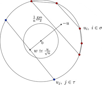
Adding new contact points.

Note that
 $$\begin{eqnarray}\biggl(\mathop{\sum }_{j\in \unicode[STIX]{x1D70E}}c_{j}\biggr)(-u)=\mathop{\sum }_{j\in \unicode[STIX]{x1D70E}}c_{j}u_{j},\end{eqnarray}$$
and this shows that
 $-u\in \text{conv}\{u_{j}:j\in \unicode[STIX]{x1D70E}\}$
(see Figure 1). It follows that the segment
 $$\begin{eqnarray}\biggl[-u,\frac{u}{\sqrt{\unicode[STIX]{x1D700}n}}\biggr]\subset \text{conv}\{u_{j}:j\in \unicode[STIX]{x1D70E}\cup \unicode[STIX]{x1D70F}\}.\end{eqnarray}$$
For
 $j\in \unicode[STIX]{x1D70E}$
, we set
 $$\begin{eqnarray}v_{j}=\sqrt{\frac{n}{n+1}}\biggl(-u_{j},\frac{1}{\sqrt{n}}\biggr)\in \mathbb{R}^{n+1}\qquad \text{and}\qquad b_{j}=\frac{n+1}{n}c_{j}.\end{eqnarray}$$
We also set
 $-v=\sqrt{n/(n+1)}(u,0)$
. Then, using (6.17), we get
 $$\begin{eqnarray}\mathop{\sum }_{j\in \unicode[STIX]{x1D70E}}b_{j}(v_{j}+v)\otimes (v_{j}+v)=\left(\begin{array}{@{}cc@{}}\mathop{\sum }_{j\in \unicode[STIX]{x1D70E}}c_{j}(u_{j}+u)\otimes (u_{j}+u) & 0\\ 0 & \frac{\mathop{\sum }_{j\in \unicode[STIX]{x1D70E}}c_{j}}{n}\end{array}\right),\end{eqnarray}$$
which implies, with the help of (6.19), that
 $$\begin{eqnarray}I_{n+1}\preccurlyeq \mathop{\sum }_{j\in \unicode[STIX]{x1D70E}}b_{j}(v_{j}+v)\otimes (v_{j}+v)\preccurlyeq (4+2\unicode[STIX]{x1D700})I_{n+1}.\end{eqnarray}$$
We rewrite (6.26) as follows:
 $$\begin{eqnarray}\displaystyle & & \displaystyle I_{n+1}-\mathop{\sum }_{j\in \unicode[STIX]{x1D70E}}b_{j}v_{j}\otimes v-\mathop{\sum }_{j\in \unicode[STIX]{x1D70E}}v\otimes b_{j}v_{j}-\biggl(\mathop{\sum }_{j\in \unicode[STIX]{x1D70E}}b_{j}\biggr)v\otimes v\nonumber\\ \displaystyle & & \displaystyle \quad \preccurlyeq \mathop{\sum }_{j\in \unicode[STIX]{x1D70E}}b_{j}v_{j}\otimes v_{j}\preccurlyeq (4+2\unicode[STIX]{x1D700})I_{n+1}-\mathop{\sum }_{j\in \unicode[STIX]{x1D70E}}b_{j}v_{j}\otimes v\nonumber\\ \displaystyle & & \displaystyle \qquad -\,\mathop{\sum }_{j\in \unicode[STIX]{x1D70E}}v\otimes b_{j}v_{j}-\biggl(\mathop{\sum }_{j\in \unicode[STIX]{x1D70E}}b_{j}\biggr)v\otimes v.\end{eqnarray}$$
Note that
 $$\begin{eqnarray}\displaystyle \mathop{\sum }_{j\in \unicode[STIX]{x1D70E}}b_{j}v_{j} & = & \displaystyle \sqrt{\frac{n+1}{n}}\biggl(-\!\mathop{\sum }_{j\in \unicode[STIX]{x1D70E}}c_{j}u_{j},\frac{\mathop{\sum }_{j\in \unicode[STIX]{x1D70E}}c_{j}}{\sqrt{n}}\biggr)\nonumber\\ \displaystyle & = & \displaystyle \sqrt{\frac{n+1}{n}}\biggl(\biggl(\mathop{\sum }_{j\in \unicode[STIX]{x1D70E}}c_{j}\biggr)u,\frac{\mathop{\sum }_{j\in \unicode[STIX]{x1D70E}}c_{j}}{\sqrt{n}}\biggr),\end{eqnarray}$$
so
 $$\begin{eqnarray}\displaystyle \biggl(\mathop{\sum }_{j\in \unicode[STIX]{x1D70E}}b_{j}v_{j}\biggr)\otimes v & = & \displaystyle \biggl(\biggl(\mathop{\sum }_{j\in \unicode[STIX]{x1D70E}}c_{j}\biggr)u,\frac{\mathop{\sum }_{j\in \unicode[STIX]{x1D70E}}c_{j}}{\sqrt{n}}\biggr)\otimes (-u,0)\nonumber\\ \displaystyle & = & \displaystyle \left(\begin{array}{@{}cc@{}}-(\mathop{\sum }_{j\in \unicode[STIX]{x1D70E}}c_{j})u\otimes u & 0\\ -\frac{(\mathop{\sum }_{j\in \unicode[STIX]{x1D70E}}c_{j})u}{\sqrt{n}} & 0\end{array}\right).\end{eqnarray}$$
Computing in a similar way, we finally have that
 $$\begin{eqnarray}T:=\mathop{\sum }_{j\in \unicode[STIX]{x1D70E}}b_{j}v_{j}\otimes v+\mathop{\sum }_{j\in \unicode[STIX]{x1D70E}}v\otimes b_{j}v_{j}+\biggl(\mathop{\sum }_{j\in \unicode[STIX]{x1D70E}}b_{j}\biggr)v\otimes v=\left(\begin{array}{@{}cc@{}}V & z\\ z & 0\end{array}\right),\end{eqnarray}$$
where
 $V=-(\sum _{j\in \unicode[STIX]{x1D70E}}c_{j})u\otimes u$
and
 $z=-(\sum _{j\in \unicode[STIX]{x1D70E}}c_{j})u/\sqrt{n}$
. Now, for every
 $(x,t)\in S^{n}$
, we have
 $$\begin{eqnarray}\displaystyle \langle T(x,t),(x,t)\rangle & = & \displaystyle \langle Vx,x\rangle +2t\langle z,x\rangle \leqslant \Vert V\Vert +2\Vert z\Vert _{2}\nonumber\\ \displaystyle & = & \displaystyle \biggl(\mathop{\sum }_{j\in \unicode[STIX]{x1D70E}}c_{j}\biggr)\Vert u\Vert _{2}^{2}+\biggl(\mathop{\sum }_{j\in \unicode[STIX]{x1D70E}}c_{j}\biggr)\frac{2\Vert u\Vert _{2}}{\sqrt{n}}\leqslant \unicode[STIX]{x1D700}+(4+2\unicode[STIX]{x1D700})n\frac{2\sqrt{\unicode[STIX]{x1D700}}}{n}\nonumber\\ \displaystyle & = & \displaystyle \unicode[STIX]{x1D700}+2\sqrt{\unicode[STIX]{x1D700}}(4+2\unicode[STIX]{x1D700}).\end{eqnarray}$$
Choosing
 $\unicode[STIX]{x1D700}=10^{-3}$
, we get
 $$\begin{eqnarray}\biggl\|\mathop{\sum }_{j\in \unicode[STIX]{x1D70E}}b_{j}v_{j}\otimes v+\mathop{\sum }_{j\in \unicode[STIX]{x1D70E}}v\otimes b_{j}v_{j}+\biggl(\mathop{\sum }_{j\in \unicode[STIX]{x1D70E}}b_{j}\biggr)v\otimes v\biggr\|\leqslant \frac{1}{2},\end{eqnarray}$$
and going back to (6.27) we get
 $$\begin{eqnarray}\frac{1}{2}I_{n+1}\preccurlyeq \mathop{\sum }_{j\in \unicode[STIX]{x1D70E}}b_{j}v_{j}\otimes v_{j}\preccurlyeq 5I_{n+1}.\end{eqnarray}$$
Now we apply Theorem 5.3 to find
 $\unicode[STIX]{x1D705}_{j}>0$
,
 $j\in \unicode[STIX]{x1D70E}$
, such that if
 $f_{j}:\mathbb{R}\rightarrow \mathbb{R}^{+}$
are integrable functions, then
 $$\begin{eqnarray}\int _{\mathbb{R}^{n+1}}\mathop{\prod }_{j\in \unicode[STIX]{x1D70E}}f_{j}^{\unicode[STIX]{x1D705}_{j}}(\langle y,v_{j}\rangle )\,dy\leqslant 10^{(n+1)/2}\mathop{\prod }_{j\in \unicode[STIX]{x1D70E}}\biggl(\int _{\mathbb{R}}f_{j}(t)\,dt\biggr)^{\unicode[STIX]{x1D705}_{j}}.\end{eqnarray}$$
For
 $j\in \unicode[STIX]{x1D70E}$
, we define
 $f_{j}(t)=\text{e}^{-(b_{j}/\unicode[STIX]{x1D705}_{j})t}\mathbf{1}_{[0,\infty )}(t)$
. Then
 $$\begin{eqnarray}\displaystyle \int _{\mathbb{R}^{n+1}}\mathop{\prod }_{j\in \unicode[STIX]{x1D70E}}f_{j}^{\unicode[STIX]{x1D705}_{j}}(\langle y,v_{j}\rangle )\,dy & {\leqslant} & \displaystyle 10^{(n+1)/2}\mathop{\prod }_{j\in \unicode[STIX]{x1D70E}}\biggl(\int _{\mathbb{R}}f_{j}(t)\,dt\biggr)^{\unicode[STIX]{x1D705}_{j}}\nonumber\\ \displaystyle & = & \displaystyle 10^{(n+1)/2}\mathop{\prod }_{j\in \unicode[STIX]{x1D70E}}\biggl(\frac{\unicode[STIX]{x1D705}_{j}}{b_{j}}\biggr)^{\unicode[STIX]{x1D705}_{j}}\leqslant 40^{(n+1)/2},\end{eqnarray}$$
recalling from Proposition 5.2 that
 $\unicode[STIX]{x1D705}_{j}/b_{j}=\langle A^{-1}u_{j},u_{j}\rangle \leqslant 2$
. The last inequality is a consequence of
 ${\textstyle \frac{1}{2}}I_{n+1}\preccurlyeq A=\sum _{j\in \unicode[STIX]{x1D70E}}b_{j}v_{j}\otimes v_{j}$
.
Let
 $$\begin{eqnarray}Q=\{x\in \mathbb{R}^{n}:\langle x,u_{j}\rangle <1,j\in \unicode[STIX]{x1D70E}\cup \unicode[STIX]{x1D70F}\}.\end{eqnarray}$$
We write
 $y=(x,r)\in \mathbb{R}^{n+1}$
and assume that
 $r>0$
and
 $x\in (r/\sqrt{n})Q$
. Then we have
 $\langle x,u_{j}\rangle <r/\sqrt{n}$
for all
 $j\in \unicode[STIX]{x1D70E}$
. This implies that
 $\langle y,v_{j}\rangle >0$
for all
 $j\in \unicode[STIX]{x1D70E}$
and hence
 $\prod _{j\in \unicode[STIX]{x1D70E}}f_{j}^{\unicode[STIX]{x1D705}_{j}}(\langle y,v_{j}\rangle )>0$
. We also have
 $$\begin{eqnarray}\displaystyle \frac{1}{(\mathop{\sum }_{j\in \unicode[STIX]{x1D70E}}c_{j})}\langle \mathop{\sum }_{j\in \unicode[STIX]{x1D70E}}c_{j}u_{j},x\rangle & = & \displaystyle \langle -u,x\rangle =\sqrt{\unicode[STIX]{x1D700}n}\langle -w,x\rangle =\sqrt{\unicode[STIX]{x1D700}n}\langle -\!\mathop{\sum }_{i\in \unicode[STIX]{x1D70F}}\unicode[STIX]{x1D70C}_{i}u_{i},x\rangle \nonumber\\ \displaystyle & {\geqslant} & \displaystyle -\sqrt{\unicode[STIX]{x1D700}}r,\end{eqnarray}$$
where the last inequality holds since
 $x\in (r/\sqrt{n})Q$
. It follows that
 $$\begin{eqnarray}\langle \mathop{\sum }_{j\in \unicode[STIX]{x1D70E}}c_{j}u_{j},x\rangle \geqslant -5\sqrt{\unicode[STIX]{x1D700}}rn.\end{eqnarray}$$
Using the above (and recalling our choice of
 $\unicode[STIX]{x1D700}=10^{-3}<1$
), we see that if
 $y=(x,r)\in (r/\sqrt{n})Q\times (0,\infty )$
, then
 $$\begin{eqnarray}\displaystyle \mathop{\prod }_{j\in \unicode[STIX]{x1D70E}}f_{j}^{\unicode[STIX]{x1D705}_{j}}(\langle y,v_{j}\rangle ) & = & \displaystyle \exp \biggl(-\!\mathop{\sum }_{j\in \unicode[STIX]{x1D70E}}b_{j}\biggl(\frac{r}{\sqrt{n+1}}-\sqrt{\frac{n}{n+1}}\langle x,u_{j}\rangle \biggr)\biggr)\nonumber\\ \displaystyle & = & \displaystyle \exp \biggl(-\frac{r}{\sqrt{n+1}}\mathop{\sum }_{j\in \unicode[STIX]{x1D70E}}b_{j}\biggr)\exp \biggl(\sqrt{\frac{n+1}{n}}\langle x,\mathop{\sum }_{j\in \unicode[STIX]{x1D70E}}c_{j}u_{j}\rangle \biggr)\nonumber\\ \displaystyle & {\geqslant} & \displaystyle \exp (-5r\sqrt{n+1}-5\sqrt{\unicode[STIX]{x1D700}}r(n+1))\nonumber\\ \displaystyle & {\geqslant} & \displaystyle \exp (-10r(n+1)).\end{eqnarray}$$
Now (6.35) gives us
 $$\begin{eqnarray}\displaystyle \frac{\operatorname{vol}_{n}(Q)}{n^{n/2}}\int _{0}^{\infty }r^{n}\text{e}^{-10r(n+1)}\,dr & = & \displaystyle \int _{0}^{\infty }\int _{(r/\sqrt{n})Q}\text{e}^{-10r(n+1)}\,dx\,dr\nonumber\\ \displaystyle & {\leqslant} & \displaystyle \int _{\mathbb{R}^{n+1}}\mathop{\prod }_{j\in \unicode[STIX]{x1D70E}}f_{j}^{\unicode[STIX]{x1D705}_{j}}(\langle y,v_{j}\rangle )\,dy\nonumber\\ \displaystyle & {\leqslant} & \displaystyle 40^{(n+1)/2}.\end{eqnarray}$$
Direct computation and then Stirling’s approximation show that
 $$\begin{eqnarray}\operatorname{vol}_{n}(Q)\leqslant C_{1}^{n}\frac{n^{3n/2}}{n!}\leqslant C_{2}^{n}n^{n/2}\end{eqnarray}$$
and
 $Q$
is the intersection of at most
 $|\unicode[STIX]{x1D70E}|+|\unicode[STIX]{x1D70F}|\leqslant \unicode[STIX]{x1D6FC}_{1}(10^{-3})n+n+1\leqslant \unicode[STIX]{x1D6FC}n$
half-spaces, where
 $\unicode[STIX]{x1D6FC}=\unicode[STIX]{x1D6FC}_{1}(10^{-3})+2$
. Since
 $B_{2}^{n}\subseteq P$
, we get
 $$\begin{eqnarray}\operatorname{vol}_{n}(Q)\leqslant \frac{C_{2}^{n}n^{n/2}}{\text{vol}_{n}(B_{2}^{n})}\operatorname{vol}_{n}(P),\end{eqnarray}$$
and the result follows.
Acknowledgements
We would like to thank Apostolos Giannopoulos for suggesting the problem and for useful discussions. We would also like to thank the referee for comments and valuable suggestions on the presentation of the results of this article. We acknowledge support from the programme “API
 $\unicode[STIX]{x1D6F4}$
TEIA II” (ATOCB-3566, research number 70/30/12386) of the General Secretariat for Research and Technology of Greece co-financed by the European Union and Greek national funds through the Operational Programme “Education and Lifelong Learning” of the National Strategic Reference Framework (NSRF).