1 Introduction
Thin films flowing on substrates are widespread in both industrial applications and nature. Examples are the lava flow on volcanoes (Huppert et al. Reference Huppert, Shepherd, Sigurdsson and Sparks1982), the spreading of paint on walls (Eres, Schwartz & Roy Reference Eres, Schwartz and Roy2000), the spin-coating process in microchip fabrication (Scriven Reference Scriven1988) and the film of wine climbing the side of a glass (Thomson Reference Thomson1855), to name a few. Body or surface-shear forces, such as gravity (Huppert Reference Huppert1982; Takagi & Huppert Reference Takagi and Huppert2010), centrifugal forces (Tanner Reference Tanner1986; Melo, Joanny & Fauve Reference Melo, Joanny and Fauve1989; Fraysse & Homsy Reference Fraysse and Homsy1994; Wang & Chou Reference Wang and Chou2001; Schwartz & Roy Reference Schwartz and Roy2004; Holloway et al. Reference Holloway, Habdas, Semsarillar, Burfitt and de Bruyn2007) or surface-tension gradients (Cazabat et al. Reference Cazabat, Heslot, Troian and Carles1990; Brzoska, Brochard-Wyart & Rondelez Reference Brzoska, Brochard-Wyart and Rondelez1992; Kataoka & Troian Reference Kataoka and Troian1997), drive these flows, which all present a capillary ridge in the vicinity of the contact line. The moving ridge is unstable to spanwise perturbations and is at the origin of the fingering instability: the thin film destabilizes in the spanwise direction and eventually splits into separate fingers (Hocking & Miksis Reference Hocking and Miksis1993; Kondic Reference Kondic2003).
In the coating industry, the non-uniformity of liquid distribution, potentially resulting in dry patches, is a critical issue to be overcome (Kistler et al. Reference Kistler and Schweizer1997). The interest of the scientific community in driven thin-film flows has increased considerably in the last three decades, in particular after the seminal work of Huppert (Reference Huppert1982) on the viscous flow on an inclined plane. Due to the small thickness of these viscous flows, their dynamics is well described by a long-wavelength approach (Oron, Davis & Bankoff Reference Oron, Davis and Bankoff1997; Craster & Matar Reference Craster and Matar2009), where the contact line can also be taken into account (Davis Reference Davis1983) and inertia is negligible due to the small Reynolds number of the flow. Newtonian and non-Newtonian fluids have both been considered in the literature (Fraysse & Homsy Reference Fraysse and Homsy1994; Spaid & Homsy Reference Spaid and Homsy1996; de Bruyn, Habdas & Kim Reference de Bruyn, Habdas and Kim2002; Balmforth, Ghadge & Myers Reference Balmforth, Ghadge and Myers2007). The resulting nonlinear lubrication equation was first solved numerically by Schwartz (Reference Schwartz1989), showing the formation of fingers in a gravity-driven flow.
The draining film far upstream from the ridge is almost flat with thickness
 $H_{N}^{\ast }$
and the capillary pressure can be neglected. This region is usually called the outer region. The body force, or the surface-shear force, balances the viscous stresses and the film profile is given by a self-similar solution for a fixed fluid quantity (Huppert Reference Huppert1982), which finishes abruptly at the front location. There, in reality, the film profile is regularized by surface tension. In this inner region close to the contact line, surface-tension effects have to be considered together with the body force, or surface-shear stresses, and with the viscous stresses. The upstream boundary condition for the inner solution is found by matching its film thickness to that of the outer solution,
 $H_{N}^{\ast }$
, whereas the boundary condition at the downstream region requires the modelling of the contact line. Spaid & Homsy (Reference Spaid and Homsy1996) have shown that a precursor film model or a slip model can both be used without impacting the value of the most amplified wavelength. The detailed flow field in the vicinity of the contact line has been computed by Goodwin & Homsy (Reference Goodwin and Homsy1991). Brenner (Reference Brenner1993) first pointed out that the instability mechanism is driven by the macroscopic feature of the capillary ridge profile and is not significantly influenced by the contact-line dynamics. A composite solution (Van Dyke Reference Van Dyke1975) valid over the entire domain has been proposed by Moriarty, Schwartz & Tuck (Reference Moriarty, Schwartz and Tuck1991).
The first precise description of the inner solution for the gravity-driven flow of Huppert (Reference Huppert1982) has been given by Troian et al. (Reference Troian, Herbolzheimer, Safran and Joanny1989) and Hocking (Reference Hocking1990). In contrast to the solution in the outer region, which follows a self-similar solution (Huppert Reference Huppert1982), the solution in the inner region can be assumed as quasi-static and corresponds to a travelling wave solution (Bertozzi & Brenner Reference Bertozzi and Brenner1997). Due to the stationarity of the base-state solution in the inner region, a classical modal stability analysis can be performed. The linearly most amplified spanwise wavelength scales as
 $\unicode[STIX]{x1D706}^{\ast }\sim \ell ^{\ast }$
, where
 $\ell ^{\ast }=H_{N}^{\ast }(3Ca)^{-1/3}$
is the characteristic length of the ridge, with
 $Ca$
being the capillary number defined with the front advancing velocity (Spaid & Homsy Reference Spaid and Homsy1996).
A detailed study of the instability mechanism has been performed by Spaid & Homsy (Reference Spaid and Homsy1996) using energy calculations. They showed that the fingering instability is mainly driven by how the perturbed free-surface base state responds to the body force: thicker regions travel faster than thin regions as they experience less viscous friction, promoting the formation of fingers. The variations in the spanwise curvature of the free surface are, on the other hand, responsible for the determination of the cut-off wavenumber.
Furthermore, it has been shown that the microscopic scale perturbation at the contact line might experience a transient growth sufficiently large to modify the macroscopic structure of the ridge and thus affect the formation of fingers (Bertozzi & Brenner Reference Bertozzi and Brenner1997). The reason is the singular dependence of the base state on the microscopic length scale at the contact line. This mechanism might explain the irregularity of the observed patterns in experiments, which are very sensitive to substrate inhomogeneities.
In contrast to the commonly considered case of a fixed fluid quantity spreading over a substrate, for which the outer solution is time dependent, when the flow is continuously fed, the outer solution is stationary (Tuck & Schwartz Reference Tuck and Schwartz1990). This configuration has been investigated in great detail by Eres et al. (Reference Eres, Schwartz and Roy2000) and Kondic & Diez (Reference Kondic and Diez2001).
However, there are also flow configurations where not only is the outer solution time dependent, but also the inner solution cannot be considered as quasi-static. This is for example the case of the flow over a curved substrate (Takagi & Huppert Reference Takagi and Huppert2010), where the forces acting on the advancing ridge vary depending on its location. The same is true for the spin-coating problem, where the centrifugal forces are space dependent. Therefore, in these cases, the stability analysis is more complex and a classical normal mode decomposition leading to an eigenvalue problem cannot be performed. The physical reason is that the most unstable mode cannot grow exponentially in time as an eigenmode since the base flow on which it evolves is modified in time, and is not a travelling wave solution. Hence, the most amplified perturbation at one time instant will not be effective at the following time, when the forces at play will be different. So far, the stability properties of these complex configurations have been investigated mostly either by experiments (Wang & Chou Reference Wang and Chou2001; Takagi & Huppert Reference Takagi and Huppert2010) or by numerical simulations (Schwartz & Roy Reference Schwartz and Roy2004), but a complete stability analysis for these time- and space-dependent flows is still lacking. Fraysse & Homsy (Reference Fraysse and Homsy1994) successfully compared the linear growth predicted by the linear theory for a quasi-steady base state (Troian et al. Reference Troian, Herbolzheimer, Safran and Joanny1989) with their experimental results of a film spreading under centrifugal forces. Nevertheless, they had to provide the critical radius where the fingers form, i.e. the critical time for the onset of the instability, as an input parameter.
Inspired by the work of Takagi & Huppert (Reference Takagi and Huppert2010), we investigate here the fingering instability on a cylindrical substrate by performing a linear optimal transient growth analysis. Given the spatial variations of the forces at play, the characteristics of the draining flow, as the length of the capillary ridge, vary in space and time. Non-modal approaches have been proven to be effective in predicting stability properties of time-evolving flows (Schmid Reference Schmid2007), also in the context of thin films (Balestra, Brun & Gallaire Reference Balestra, Brun and Gallaire2016). In the present work, we consider two distinct optimization problems. First, we look for the optimal initial condition of the film-thickness perturbations for a flow draining on a smooth cylindrical substrate. Second, we aim at finding the optimal perturbations of the substrate topography. The gain function to be optimized at finite times corresponds to the energy of the film-thickness perturbations, normalized by the initial thickness or substrate-perturbation energy, for the first and second problem, respectively. Substrate and film-thickness perturbations are assumed to be of the same order. We show that, for both problems, the optimal perturbations correspond to the perturbations which are the least affected by the time horizon, i.e. the time for which they are optimized, and are thus the most universal. A correct prediction of the most amplified pattern is only possible by considering the transient dynamics of the flow, which underlines the importance of these non-modal approaches in the study of time-dependent flows.
The paper is structured as follows. The considered problem and the governing equations are presented in § 2. In § 3, we describe the axially invariant draining flow. More precisely, the lubrication equation and the initial condition are specified in § 3.1, followed by the description of the drainage at the pole (§ 3.2), the approximate solution for the outer region (§ 3.3), the spatio-temporal dependence of the front location (§ 3.4) and the evolution of the capillary-ridge length (§ 3.5). The optimal transient growth analysis for the initial film-thickness perturbations is presented in § 4, starting with the decomposition into base state and perturbations in § 4.1, the linear disturbance equation in § 4.2 and the optimization method in § 4.3. The results follow in § 4.4, where the effect of the time horizon is given in § 4.4.1 and that of the spanwise wavenumber in § 4.4.2. The modification of the lubrication equation due to the substrate-topography perturbations is discussed in § 5.1, followed by the decomposition of the free-surface elevation in § 5.2 and the linearization in § 5.3. The optimization method is described in § 5.4 and the results are given in § 5.5. Conclusions are drawn in § 6.
2 Problem formulation and governing equations
Consider the instantaneous release of a Newtonian fluid of dynamic viscosity
 $\unicode[STIX]{x1D707}$
and density
 $\unicode[STIX]{x1D70C}$
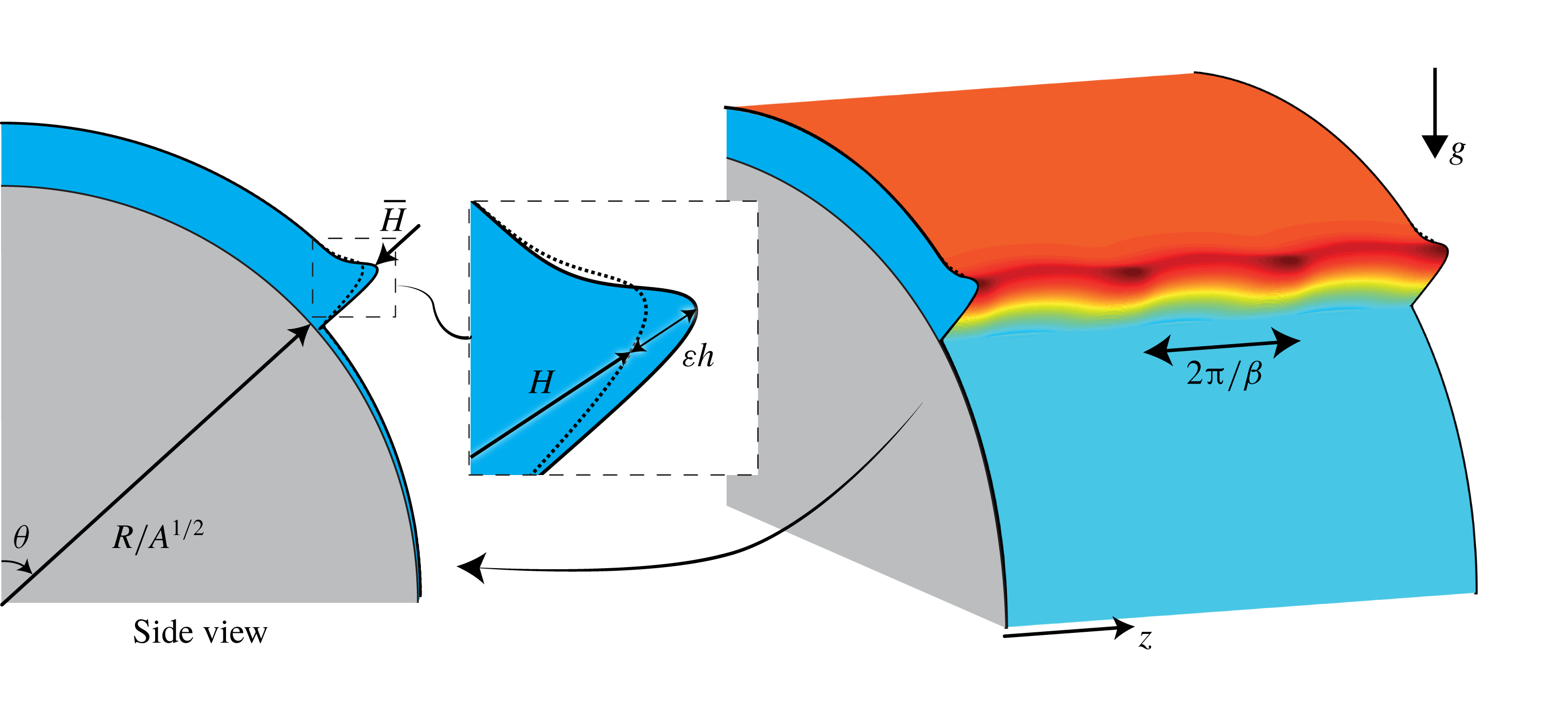
spreading on the outside of a smooth cylindrical substrate of radius
 $R$
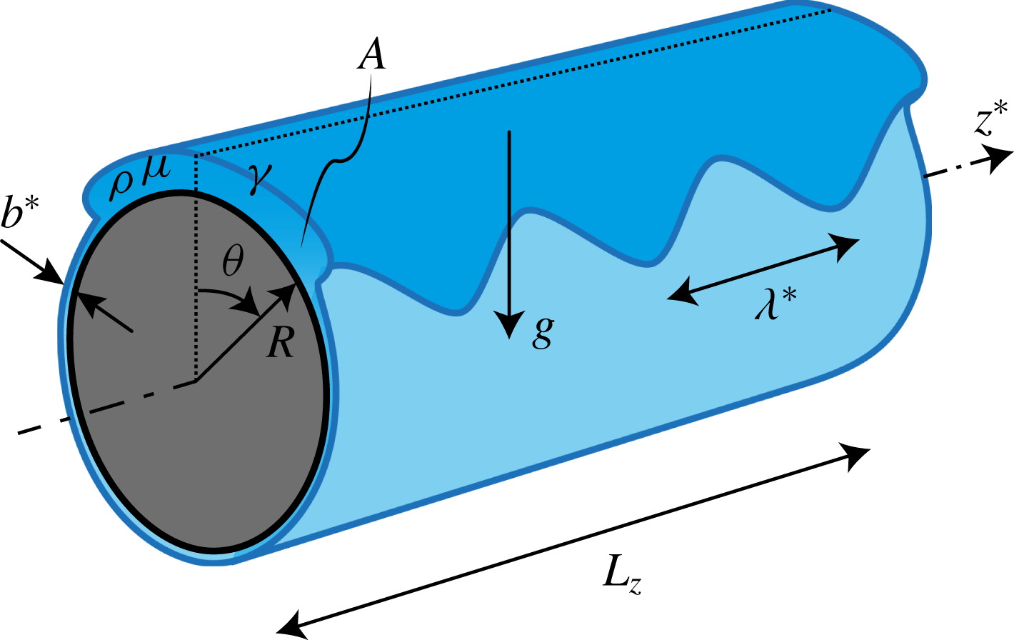
whose axis is orthogonal to gravity (see figure 1). The fluid is pulled by the gravitational field
 $g$
and slowed down by viscous friction.
Sketch of the considered problem geometry.

The fluid thickness profile is initially invariant in the axial direction and the cross-sectional area is
 $A$
. Under the assumption of a small film aspect ratio
 $\unicode[STIX]{x1D6FF}=\sqrt{A}/R\ll 1$
we can use the long-wavelength approximation to describe this flow (Oron et al.
Reference Oron, Davis and Bankoff1997). Given the small Reynolds number
 $Re=g\unicode[STIX]{x1D70C}^{2}A^{3/2}/(3\unicode[STIX]{x1D707}^{2})$
, inertial effects can be neglected and the Stokes equations in polar coordinates
 $(r^{\ast },\unicode[STIX]{x1D703},z^{\ast })$
can be integrated over the radial direction to obtain, using mass conservation, the lubrication equation for the film thickness
 $\bar{H}^{\ast }(\unicode[STIX]{x1D703},z^{\ast },t^{\ast })$
(see Balestra et al. (Reference Balestra, Kofman, Brun, Scheid and Gallaire2017) for a detailed derivation)
 $$\begin{eqnarray}\displaystyle & & \displaystyle \bar{H}_{t^{\ast }}^{\ast }+\frac{1}{3\unicode[STIX]{x1D707}R}\left[\bar{H}^{\ast 3}\left(\underbrace{\frac{\unicode[STIX]{x1D6FE}\bar{\unicode[STIX]{x1D705}}_{\unicode[STIX]{x1D703}}^{\ast }}{R}}_{\text{I}}-\underbrace{\frac{\unicode[STIX]{x1D70C}g\cos \unicode[STIX]{x1D703}\bar{H}_{\unicode[STIX]{x1D703}}^{\ast }}{R}}_{\text{II}}+\underbrace{\unicode[STIX]{x1D70C}g\sin \unicode[STIX]{x1D703}}_{\text{III}}\right)\right]_{\unicode[STIX]{x1D703}}\nonumber\\ \displaystyle & & \displaystyle \quad +\,\frac{1}{3\unicode[STIX]{x1D707}}\left[\bar{H}^{\ast 3}\left(\underbrace{\unicode[STIX]{x1D6FE}\bar{\unicode[STIX]{x1D705}}_{z^{\ast }}^{\ast }}_{\text{I}}-\underbrace{\unicode[STIX]{x1D70C}g\cos \unicode[STIX]{x1D703}\bar{H}_{z^{\ast }}^{\ast }}_{\text{II}}\right)\right]_{z^{\ast }}=0,\end{eqnarray}$$
where
 $\unicode[STIX]{x1D6FE}$
is the surface tension,
 $\bar{\unicode[STIX]{x1D705}}^{\ast }=-\unicode[STIX]{x1D735}^{\ast }\boldsymbol{\cdot }\boldsymbol{n}^{\ast }$
is the curvature of the interface with normal vector
 $\boldsymbol{n}^{\ast }=\unicode[STIX]{x1D735}^{\ast }F/\Vert \unicode[STIX]{x1D735}^{\ast }F\Vert$
and
 $F=r^{\ast }-(R+\bar{H}^{\ast })=0$
defines the free surface; subscripts correspond to partial derivatives. Term
 $\text{I}$
corresponds to the capillary pressure gradient, term
 $\text{II}$
to the variation of the hydrostatic pressure and term
 $\text{III}$
to the drainage. The term
 $\bar{H}^{\ast 3}$
is the mobility of the liquid and results from the integration of the half-Poiseuille velocity profile in the thin film. The only difference from the lubrication equation for a thin film coating the inside of a cylindrical substrate used in Balestra et al. (Reference Balestra, Kofman, Brun, Scheid and Gallaire2017) is the sign of the hydrostatic pressure variation. In the present geometry, the variation of the hydrostatic pressure is stabilizing for
 $\unicode[STIX]{x1D703}\in [\!0,\unicode[STIX]{x03C0}/2\ $\unicode[STIX]{x1D703}\in ]\!\unicode[STIX]{x03C0}/2,\unicode[STIX]{x03C0}\!]$
. On the lower external part of the cylinder, not considered in this study, the liquid will accumulate in rivulets due to the Rayleigh–Taylor instability, eventually forming dripping droplets (Duffy & Moffatt Reference Duffy and Moffatt1995; Indeikina, Veretennikov & Chang Reference Indeikina, Veretennikov and Chang1997; Takagi & Huppert Reference Takagi and Huppert2010; Lin, Kondic & Filippov Reference Lin, Kondic and Filippov2012; Leslie, Wilson & Duffy Reference Leslie, Wilson and Duffy2013; Paterson, Wilson & Duffy Reference Paterson, Wilson and Duffy2014). The problem being symmetric with respect to
 $\unicode[STIX]{x1D703}=0$
, only half of the cylinder is considered.
The scalings used in this work are chosen to agree with previous studies. Length
 $L=\sqrt{A}$
is the characteristic length in the radial direction and
 $\unicode[STIX]{x1D70F}_{d}=\unicode[STIX]{x1D707}R/(\unicode[STIX]{x1D70C}gA)$
is the characteristic drainage time, which results from the ratio of the viscous over the gravitational stresses (Takagi & Huppert Reference Takagi and Huppert2010; Trinh et al.
Reference Trinh, Kim, Hammoud, Howell, Chapman and Stone2014). As a side remark, note that, as pointed out by one of the referees, a probably more suitable choice of characteristic length in the radial direction and of characteristic time would have been
 $A/R$
and
 $\unicode[STIX]{x1D707}R^{3}/(\unicode[STIX]{x1D70C}gA^{2})$
, respectively. Sticking to the classic characteristic quantities previously used in the literature, the dimensionless Bond number, prescribing the ratio between the gravitational and the capillary forces, reads
 $Bo=\unicode[STIX]{x1D70C}gA^{3/2}/(\unicode[STIX]{x1D6FE}R)$
. In the present study, the considered Bond number and film aspect ratio are chosen such as to correspond to the experiment of Takagi & Huppert (Reference Takagi and Huppert2010); namely
 $Bo=15$
and
 $\unicode[STIX]{x1D6FF}=0.15$
. The lubrication equation can be written in the following dimensionless form:
 $$\begin{eqnarray}\displaystyle \bar{H}_{t}+\frac{1}{3}\left\{\bar{H}^{3}\left[\frac{\unicode[STIX]{x1D6FF}^{2}}{Bo}\bar{\unicode[STIX]{x1D705}}_{\unicode[STIX]{x1D703}}-\unicode[STIX]{x1D6FF}\cos \unicode[STIX]{x1D703}\bar{H}_{\unicode[STIX]{x1D703}}+\sin \unicode[STIX]{x1D703}\right]\right\}_{\unicode[STIX]{x1D703}}+\frac{1}{3\unicode[STIX]{x1D6FF}}\left\{\bar{H}^{3}\left[\frac{\unicode[STIX]{x1D6FF}}{Bo}\bar{\unicode[STIX]{x1D705}}_{z}-\cos \unicode[STIX]{x1D703}\bar{H}_{z}\right]\right\}_{z}=0. & & \displaystyle \nonumber\\ \displaystyle & & \displaystyle\end{eqnarray}$$
The different powers of
 $\unicode[STIX]{x1D6FF}$
in the axial and polar fluxes result from the different characteristic lengths in the polar and axial directions. While the characteristic length in the polar direction is
 $R$
, that in the axial direction scales like the film thickness (Troian et al.
Reference Troian, Herbolzheimer, Safran and Joanny1989) and is thus
 $\sqrt{A}$
. Note that the three essential physical ingredients, namely the capillary pressure gradient, the variation of the hydrostatic pressure and the drainage, appear at different orders in
 $\unicode[STIX]{x1D6FF}$
. Following Takagi & Huppert (Reference Takagi and Huppert2010) and Trinh et al. (Reference Trinh, Kim, Hammoud, Howell, Chapman and Stone2014), the principle of least degeneracy (Van Dyke Reference Van Dyke1975) has been used and only the leading-order terms in
 $\unicode[STIX]{x1D6FF}$
of the different physical ingredients have been considered. The full curvature
 $\bar{\unicode[STIX]{x1D705}}=-\unicode[STIX]{x1D735}\boldsymbol{\cdot }\boldsymbol{n}$
is truncated at the second order in
 $\unicode[STIX]{x1D6FF}$
in order to keep only the leading-order dependence on the polar film-thickness variations:
 $$\begin{eqnarray}\displaystyle \bar{\unicode[STIX]{x1D705}}=-\unicode[STIX]{x1D6FF}+\bar{H}_{zz}+\unicode[STIX]{x1D6FF}^{2}(\bar{H}+\bar{H}_{\unicode[STIX]{x1D703}\unicode[STIX]{x1D703}}-\bar{H}_{\unicode[STIX]{x1D703}}^{2}\bar{H}_{zz})+O(\unicode[STIX]{x1D6FF}^{3}). & & \displaystyle\end{eqnarray}$$
The modifications of the lubrication (2.2) when considering a perturbed substrate are given in § 5.1, with more details in appendix B.
3 Draining base flow
3.1 Lubrication equation
The draining base flow
 $H$
on a smooth cylindrical substrate is assumed to be invariant along the axial direction, which simplifies the lubrication (2.2) to
 $$\begin{eqnarray}\displaystyle H_{t}+\frac{1}{3}\left\{H^{3}\left[\underbrace{\frac{\unicode[STIX]{x1D6FF}^{4}}{Bo}(H_{\unicode[STIX]{x1D703}}+H_{\unicode[STIX]{x1D703}\unicode[STIX]{x1D703}\unicode[STIX]{x1D703}})}_{\text{I}}-\underbrace{\unicode[STIX]{x1D6FF}\cos \unicode[STIX]{x1D703}H_{\unicode[STIX]{x1D703}}}_{\text{II}}+\underbrace{\sin \unicode[STIX]{x1D703}}_{\text{III}}\right]\right\}_{\unicode[STIX]{x1D703}}=0. & & \displaystyle\end{eqnarray}$$
The considered initial condition is
 $$\begin{eqnarray}\displaystyle H_{0}(\unicode[STIX]{x1D703})=c_{1}\{1-\tanh [c_{2}(\unicode[STIX]{x1D703}-\unicode[STIX]{x1D719})]\}+b, & & \displaystyle\end{eqnarray}$$
where
 $c_{1}$
is the dimensionless amplitude yielding a dimensionless fluid’s area of unity,
 $\int _{0}^{\unicode[STIX]{x03C0}/2}[H_{0}(\unicode[STIX]{x1D703})-b]\,\text{d}\unicode[STIX]{x1D703}/\unicode[STIX]{x1D6FF}=1$
,
 $c_{2}=15$
sets the initial slope of the front, located for
 $t=0$
at
 $\unicode[STIX]{x1D703}=\unicode[STIX]{x1D719}=19^{\circ }$
, and
 $b$
is the precursor film thickness. Note that the fluid in the precursor film is removed in the measure of the volume. As will become clear in § 3.4, the base-flow solution at late times does not depend on the initial condition. The draining-flow lubrication (3.1) is solved over the full domain
 $\unicode[STIX]{x1D703}\in [0,\unicode[STIX]{x03C0}]$
with the boundary conditions
 $H_{\unicode[STIX]{x1D703}}=H_{\unicode[STIX]{x1D703}\unicode[STIX]{x1D703}\unicode[STIX]{x1D703}}=0$
at both ends, such that the flux vanishes at these locations. In order to avoid the unstable Rayleigh–Taylor regime, we only solve the lubrication equation until the advancing front reaches
 $\unicode[STIX]{x1D703}=\unicode[STIX]{x03C0}/2$
.
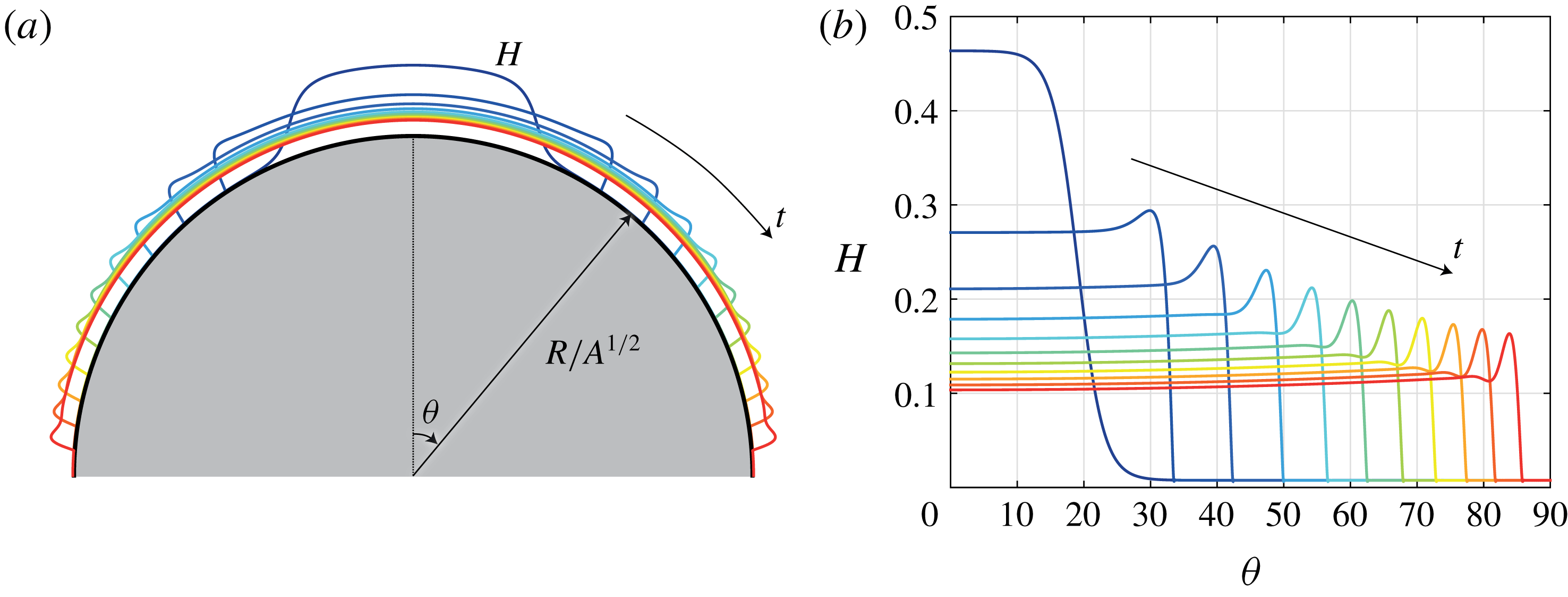
Base flow temporal evolution for
 $Bo=15$
and
 $\unicode[STIX]{x1D6FF}=0.15$
, shown in polar coordinates (a) and cartesian coordinates (b). The parameters are taken such as to have the same dimensionless numbers as in the experiment of Takagi & Huppert (Reference Takagi and Huppert2010). The film thickness in (a) has been magnified by a factor of
 $3$
for visualization purposes.

A typical evolution of the base flow is shown in figure 2 (see appendix C for details of the numerical method). The drainage solution given by (3.1) can be decomposed into an outer region where the drainage term
 $\text{III}$
dominates and an inner region close to the front where the capillary pressure and variation of hydrostatic pressure terms
 $\text{I}$
and
 $\text{II}$
, respectively, are no longer negligible (Takagi & Huppert Reference Takagi and Huppert2010).
3.2 Drainage at the pole
In the outer region close to the pole at
 $\unicode[STIX]{x1D703}=0$
, the lubrication (3.1) with negligible capillary pressure and variation of hydrostatic pressure terms can be simplified assuming the leading-order approximation
 $\sin \unicode[STIX]{x1D703}\sim \unicode[STIX]{x1D703}$
for the drainage term. Following Takagi & Huppert (Reference Takagi and Huppert2010), the resulting equation can be solved analytically and the film thickness at the pole with initial value
 $e=H_{0}(\unicode[STIX]{x1D703}=0)$
evolves as
 $$\begin{eqnarray}\displaystyle H(\unicode[STIX]{x1D703}=0,t)=\frac{1}{\sqrt{\displaystyle \frac{1}{e^{2}}+\frac{2}{3}t}}. & & \displaystyle\end{eqnarray}$$
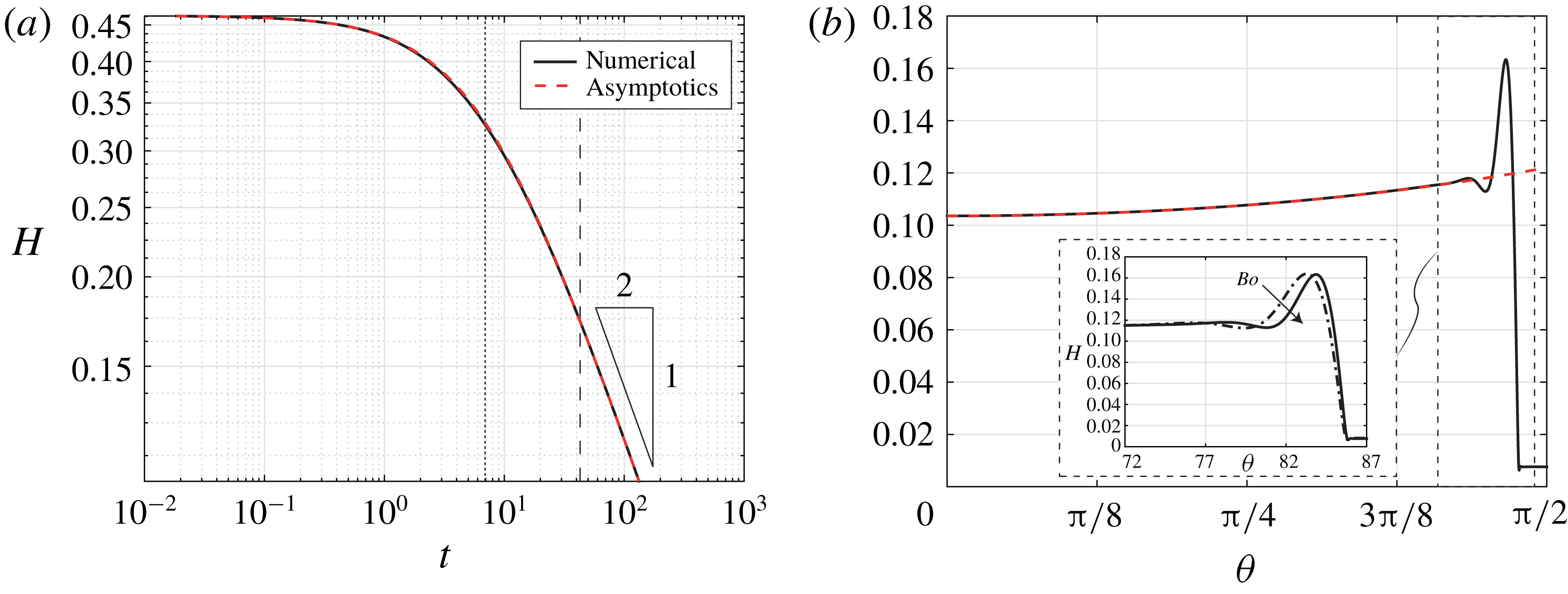
The drainage becomes independent of initial condition and follows the universal law
 $H\sim (2t/3)^{-1/2}$
for large times
 $t\gg \unicode[STIX]{x1D70F}_{i}=3/(2e^{2})$
, as visible in figure 3(a).
(a) Comparison between the temporal film thickness evolution at the pole
 $\unicode[STIX]{x1D703}=0$
obtained numerically (black solid line) and the prediction (3.3) (red dashed line). The dotted line indicates the critical initial time
 $\unicode[STIX]{x1D70F}_{i}=3/(2e^{2})$
and the dashed line the crossover time at which
 $\ell _{c}=\ell$
. (b) Comparison between the film thickness profile at
 $t=133$
obtained numerically (black solid line) and the prediction (3.4) (red dashed line). Inset: zoom in the inner region. Here
 $Bo=15$
(and
 $Bo=8$
for the dot-dashed line in the inset) and
 $\unicode[STIX]{x1D6FF}=0.15$
.

3.3 Spatial dependence of the outer region
The spatial variation of the film thickness in the outer region can be found by a regular perturbation expansion as described in Balestra et al. (Reference Balestra, Kofman, Brun, Scheid and Gallaire2017). Under the assumption of negligible capillary pressure and hydrostatic pressure contributions, the approximate solution for the film thickness up to the fourth order in
 $\unicode[STIX]{x1D703}$
reads
 $$\begin{eqnarray}\displaystyle & & \displaystyle H(\unicode[STIX]{x1D703},t)=\frac{1}{\sqrt{\displaystyle \frac{1}{e^{2}}+\frac{2}{3}t}}\left\{1+\frac{\unicode[STIX]{x1D703}^{2}}{16}\left[1-\frac{1}{\left(\displaystyle \frac{1}{e^{2}}+\frac{2}{3}t\right)^{4}}\right]\right.\nonumber\\ \displaystyle & & \displaystyle \quad +\,\left.\frac{43\unicode[STIX]{x1D703}^{4}}{10752}\left[1+\frac{315}{43\left(\displaystyle \frac{1}{e^{2}}+\frac{2}{3}t\right)^{8}}-\frac{288}{43\left(\displaystyle \frac{1}{e^{2}}+\frac{2}{3}t\right)^{7}}-\frac{70}{43\left(\displaystyle \frac{1}{e^{2}}+\frac{2}{3}t\right)^{4}}\right]\right\}+O(\unicode[STIX]{x1D703}^{6}).\nonumber\\ \displaystyle & & \displaystyle\end{eqnarray}$$
Note that the equivalent expression for the draining flow on a spherical substrate has been proven to be in excellent agreement with experimental measurements by Lee et al. (Reference Lee, Brun, Marthelot, Balestra, Gallaire and Reis2016). The very good agreement between the numerical solution of the full lubrication (3.1) and the prediction (3.4) (see figure 3 b) clearly indicates that the capillary pressure and the variation of hydrostatic pressure are negligible in the outer region.
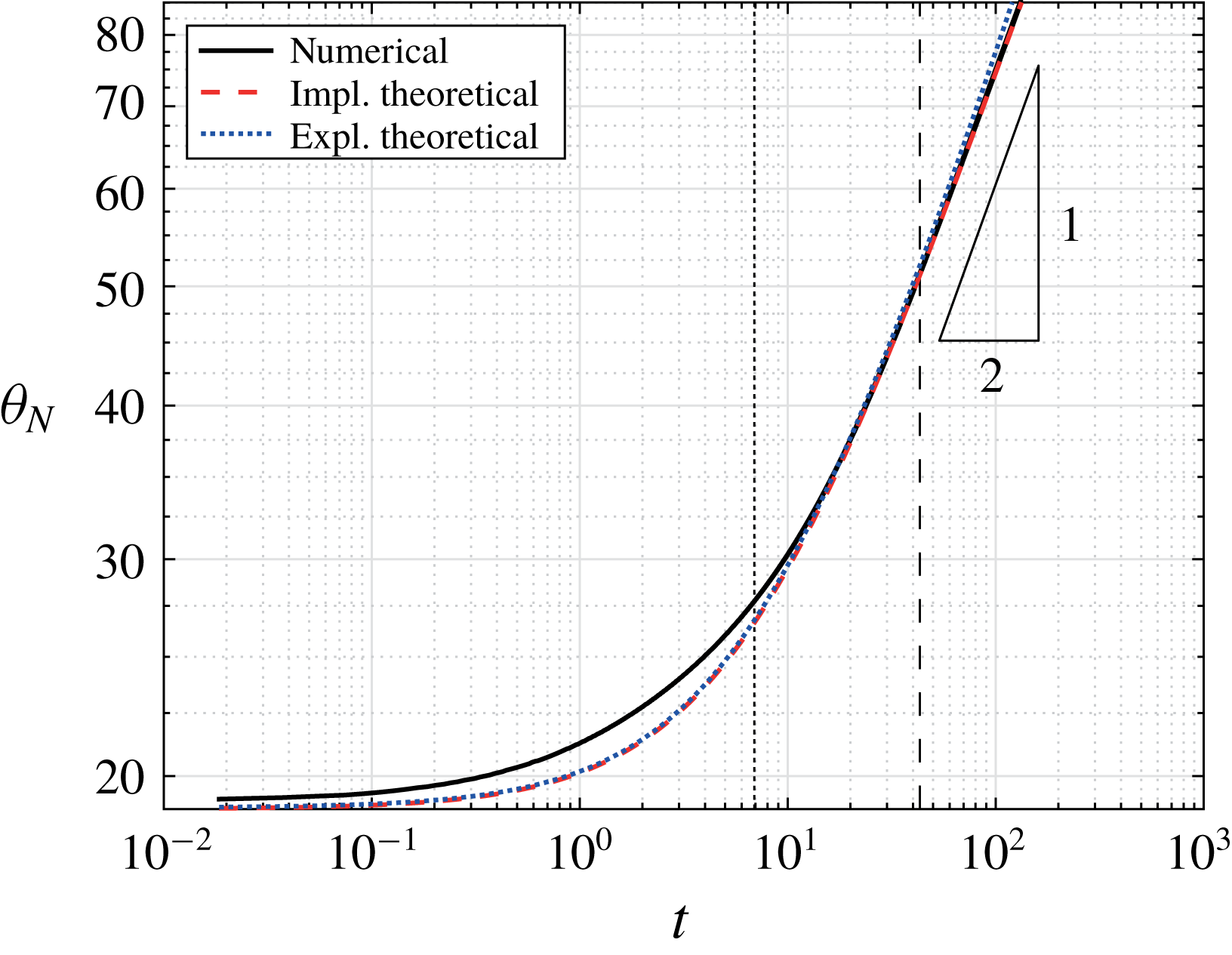
Comparison between the evolution of the front position
 $\unicode[STIX]{x1D703}_{N}$
obtained numerically (black solid line), theoretically (red dashed line) and with the explicit theoretical expression (3.6) (blue dotted line). Here
 $Bo=15$
and
 $\unicode[STIX]{x1D6FF}=0.15$
. The black dotted line indicates the critical initial time
 $\unicode[STIX]{x1D70F}_{i}=3/(2e^{2})$
and the black dashed line the crossover time at which
 $\ell _{c}=\ell$
. The front location deduced from the numerical results is arbitrarily chosen to correspond to the location where the film thickness is
 $H_{N}=[H(\unicode[STIX]{x1D703}=0,t)+b]/2$
.

3.4 Front position
The viscous liquid spreads on the cylinder as time evolves, following the expression (3.4) in the outer region. Mass conservation imposes
 $$\begin{eqnarray}\displaystyle \int _{0}^{\unicode[STIX]{x1D703}_{N}}[H(\unicode[STIX]{x1D703},t)-b]\,\text{d}\unicode[STIX]{x1D703}/\unicode[STIX]{x1D6FF}=1, & & \displaystyle\end{eqnarray}$$
where the precursor film thickness is removed to avoid an increase in fluid volume when the ridge advances. Equation (3.5), together with the approximate expression for the draining flow
 $H$
, equation (3.4), can be solved to yield an implicit solution for the front position over time
 $\unicode[STIX]{x1D703}_{N}(t)$
(see figure 4). An explicit expression can be found if one assumes that the film has constant thickness
 $H_{N}=(2t/3)^{-1/2}\gg b$
. Mass conservation yields (Takagi & Huppert Reference Takagi and Huppert2010)
 $$\begin{eqnarray}\displaystyle \unicode[STIX]{x1D703}_{N}(t)=\frac{\unicode[STIX]{x1D6FF}}{H_{N}}\sim \unicode[STIX]{x1D6FF}\sqrt{\frac{2t}{3}}, & & \displaystyle\end{eqnarray}$$
which is valid for
 $3/(2e^{2})\ll t\ll 3/(2b^{2})$
. Equation (3.6) evidences the square-root dependence of the front position with time. The implicit and explicit approximate estimates for the spreading length
 $\unicode[STIX]{x1D703}_{N}$
compare well with the result of the numerical solution of (3.1) (see figure 4). It has to be stressed that these estimates rely only on the conservation of mass for the outer region, neglecting the precise profile in the inner region close to the front.
The velocity of the front is given by
 $U_{N}=\text{d}\unicode[STIX]{x1D703}_{N}/\text{d}t/\unicode[STIX]{x1D6FF}\sim (6t)^{-1/2}$
. Although the front travels on a substrate whose local inclination increases, its velocity, which scales like
 $U_{N}\sim H_{N}^{2}\sin \unicode[STIX]{x1D703}_{N}$
, reduces with time. In fact, mass conservation imposes that the film gets thinner as
 $H_{N}\sim 1/\unicode[STIX]{x1D703}_{N}$
so that the increased viscous shear overcomes the effect of the increased gravity component driving the flow.
3.5 Length of the inner region
Surface-tension effects are only relevant in the vicinity of the ridge, where the outer film thickness has to be connected to the precursor film, inducing strong film-thickness variations. The film profile in the inner region presents a shape very similar to those found for other driven films, like the ones on an inclined plane (Spaid & Homsy Reference Spaid and Homsy1996) (see inset of figure 3 b).
The characteristic length of the ridge is found by balancing the dominant terms in (3.1). At small angles
 $\unicode[STIX]{x1D703}$
, the drainage term
 $\text{III}$
is weak compared to terms
 $\text{I}$
and
 $\text{II}$
due to the large film-thickness gradients at the front. Hence, the capillary pressure term
 $\text{I}$
has to balance the variation of the hydrostatic pressure term
 $\text{II}$
. The characteristic length of the inner region is therefore
 $$\begin{eqnarray}\displaystyle \ell _{c}=\left(\frac{\unicode[STIX]{x1D6FF}}{Bo\cos \unicode[STIX]{x1D703}_{N}}\right)^{1/2}, & & \displaystyle\end{eqnarray}$$
where
 $\unicode[STIX]{x1D703}_{N}$
is the front location. Expression (3.7) is nothing else than the capillary length defined with the gravity component in the radial direction. Written in dimensional quantities, it reads
 $\ell _{c}^{\ast }=\sqrt{\unicode[STIX]{x1D6FE}/(\unicode[STIX]{x1D70C}g\cos \unicode[STIX]{x1D703}_{N})}$
(Bertozzi & Brenner Reference Bertozzi and Brenner1997). Length
 $\ell _{c}$
is a monotonic increasing function of
 $\unicode[STIX]{x1D703}_{N}$
, and thus increases with time. For sufficiently large angles, the drainage term
 $\text{III}$
overcomes the variation of the hydrostatic pressure term
 $\text{II}$
and the film-thickness variations at the ridge occur on a length scale found by balancing the drainage term and the capillary pressure term, yielding
 $$\begin{eqnarray}\displaystyle \ell =\left(\frac{\unicode[STIX]{x1D6FF}H_{N}}{Bo\sin \unicode[STIX]{x1D703}_{N}}\right)^{1/3}=\left(\frac{\unicode[STIX]{x1D6FF}^{2}}{Bo\,\unicode[STIX]{x1D703}_{N}\sin \unicode[STIX]{x1D703}_{N}}\right)^{1/3}, & & \displaystyle\end{eqnarray}$$
where conservation of mass
 $H_{N}\unicode[STIX]{x1D703}_{N}=\unicode[STIX]{x1D6FF}$
has been used. For
 $3/(2e^{2})\ll t\ll 3/(2b^{2})$
, with the use of (3.6), one obtains
 $\ell \sim (2Bo\,t/3)^{-1/3}$
, indicating that
 $\ell$
decreases with time. Equation (3.8) is equivalent to the length of the capillary ridge for a film flowing on an inclined plane,
 $\ell =H_{N}/(3Ca)^{1/3}$
, when using
 $Ca=Bo/\unicode[STIX]{x1D6FF}U_{N}$
as capillary number, with
 $U_{N}$
the velocity at the front, given by
 $U_{N}=\sin \unicode[STIX]{x1D703}_{N}H_{N}^{2}/(3\unicode[STIX]{x1D6FF})$
.
For the parameters considered in the present study, the crossover between the two regimes is found to be at
 $t\simeq 44$
. The first regime corresponds to the relaxation of the initial film thickness profile over a relatively flat substrate, whereas the second regime corresponds to the well-developed gravity-driven ridge regularized by surface tension, where the initial condition is lost and the solution follows the scaling
 $H_{N}\sim (2t/3)^{-1/2}$
.
The two regimes have been identified also for the flow over an inclined plane depending on the inclination angle (Bertozzi & Brenner Reference Bertozzi and Brenner1997). Bertozzi & Brenner (Reference Bertozzi and Brenner1997) showed that the bump of the ridge vanishes for small inclination angles due to the component of gravity orthogonal to the substrate. This is also true for the flow over a cylinder, where the bump gains in thickness as the flow evolves downstream. It can be concluded that the length of the ridge always decreases with the Bond number, whereas it increases or decreases with the polar angle, and thus with time, for the first and second regime, respectively, as already observed in figures 2 and 3.
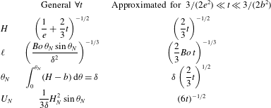
The most important scalings are summarized in table 1. The good agreement between the Bond-number-independent estimate for the film thickness
 $H$
given by (3.4) is only valid for the weak surface-tension limit, when the Bond number is sufficiently large. For very large Bond numbers, Ancey, Cochard & Andreini (Reference Ancey, Cochard and Andreini2009) showed that if surface tension is negligible everywhere, a very steep nose forms at the front. Otherwise, capillary forces will impact also the film thickness far from the ridge and the outer solution is no longer valid. Following Takagi & Huppert (Reference Takagi and Huppert2010), the present theory holds as long as
 $\unicode[STIX]{x1D703}_{N}\gg Bo^{-1/5}\unicode[STIX]{x1D6FF}$
, which is the case for the considered parameters.
Furthermore, the precursor film thickness has to be
 $b\ll e$
to avoid a non-negligible addition of mass when the ridge advances on the precursor film. In this work, we have set
 $b=8\times 10^{-3}$
, two orders of magnitude smaller than
 $e$
. With this value of
 $b$
, the upper time limit for the theory to hold is
 $3/(2b^{2})\gg t_{f}$
, where
 $t_{f}=133$
is the time at which the ridge reaches
 $\unicode[STIX]{x1D703}=\unicode[STIX]{x03C0}/2$
with the considered parameters. It has to be pointed out, however, that the precise film-thickness profile of the inner region is dependent on the exact value of the precursor film (Bertozzi & Brenner Reference Bertozzi and Brenner1997). The height of the ridge is a weak (logarithmic) function of
 $b$
(Troian et al.
Reference Troian, Herbolzheimer, Safran and Joanny1989; Tuck & Schwartz Reference Tuck and Schwartz1990). The smaller the precursor film thickness, the higher the bump and thus the stronger the growth of the perturbations. Yet, the selection of the most unstable spanwise wavenumber is not affected (Spaid & Homsy Reference Spaid and Homsy1996).
Summary of main scalings for the film thickness at the pole
 $H$
, the capillary-ridge length
 $\ell$
, the front location
 $\unicode[STIX]{x1D703}_{N}$
and its velocity
 $U_{N}$
; the general expressions valid for any time and their simplified forms for
 $3/(2e^{2})\ll t\ll 3/(2b^{2})$
are specified.

4 Optimal film thickness initial conditions over a smooth substrate
An optimal transient growth analysis is employed hereafter to find the optimal initial conditions for the film-thickness perturbations over a smooth cylindrical substrate.
4.1 Film-thickness decomposition
The numerically obtained one-dimensional draining flow discussed in § 3 is asymptotically linearly stable for
 $\unicode[STIX]{x1D703}\in [0,\unicode[STIX]{x03C0}/2]$
and can be considered as the base state for the linear stability analysis. The film thickness is decomposed into this drainage solution
 $H(\unicode[STIX]{x1D703},t)$
and small perturbations
 $\unicode[STIX]{x1D700}{\hat{h}}(\unicode[STIX]{x1D703},t)$
, with
 $\unicode[STIX]{x1D700}\ll 1$
(see figure 5):
 $$\begin{eqnarray}\displaystyle \bar{H}(\unicode[STIX]{x1D703},z,t)=\underbrace{H(\unicode[STIX]{x1D703},t)}_{drainage\;solution}+\,\underbrace{\unicode[STIX]{x1D700}{\hat{h}}(\unicode[STIX]{x1D703},z,t)}_{perturbation},\quad \unicode[STIX]{x1D700}\ll 1. & & \displaystyle\end{eqnarray}$$
Decomposition of the total film thickness
 $\bar{H}$
(solid line) into draining solution
 $H$
(dotted line) and first-order perturbations
 $\unicode[STIX]{x1D700}h\cos (\unicode[STIX]{x1D6FD}z)$
for the optimal transient growth of initial conditions
 $h_{0}$
over a smooth substrate. The spanwise perturbations with wavenumber
 $\unicode[STIX]{x1D6FD}$
are shown in the three-dimensional sketch. Here
 $\unicode[STIX]{x1D703}\in [0,\unicode[STIX]{x03C0}/2]$
and
 $z\in [0,3\times 2\unicode[STIX]{x03C0}/\unicode[STIX]{x1D6FD}]$
.

Furthermore, we assume that the perturbations are periodic in the transverse direction and we proceed to a normal mode expansion in this direction
 $$\begin{eqnarray}\displaystyle {\hat{h}}(\unicode[STIX]{x1D703},z,t)=h(\unicode[STIX]{x1D703},t)\exp (\text{i}\unicode[STIX]{x1D6FD}z)+\text{c.c.}, & & \displaystyle\end{eqnarray}$$
where
 $\unicode[STIX]{x1D6FD}\in \mathbb{R}$
is the spanwise wavenumber. The one-dimensional perturbations
 $h(\unicode[STIX]{x1D703},t)$
have to be optimized for a given spanwise wavenumber
 $\unicode[STIX]{x1D6FD}$
.
4.2 Linear disturbance equation
The linear disturbance equation governing the dynamics of the first-order perturbations
 $h(\unicode[STIX]{x1D703},t)$
is found by entering the decomposition (4.1) together with (4.2) into the nonlinear lubrication equation (2.2) and considering terms of order
 $\unicode[STIX]{x1D700}$
:
 $$\begin{eqnarray}\displaystyle h_{t}+L(H,\unicode[STIX]{x1D6FD},Bo,\unicode[STIX]{x1D6FF})h=0. & & \displaystyle\end{eqnarray}$$
The linear operator
 $L(H,\unicode[STIX]{x1D6FD},Bo,\unicode[STIX]{x1D6FF})$
is a function of the drainage solution, the spanwise wavenumber, the Bond number and the film aspect ratio (see appendix A for its expression).
4.3 Optimization method
Due to the polar and temporal dependences of the base state
 $H$
in the linear operator, the classical normal mode ansatz for
 $h$
cannot be employed (Schmid Reference Schmid2007). Instead, we use a non-modal transient growth analysis to find the largest amplification of perturbations at finite times
 $T$
, and not in the limit
 $t\rightarrow \infty$
. Bertozzi & Brenner (Reference Bertozzi and Brenner1997) have shown that in spite of the linear stability of a flow over an inclined plane at low inclination angles, a transient growth can always occur. Given the base flow drainage on a substrate whose inclination increases in space, the employed procedure is therefore suitable.
The algorithm for the optimal transient growth of the optimal initial conditions is based on the one described in Balestra et al. (Reference Balestra, Brun and Gallaire2016), and only the main steps are presented hereafter.
The energy of the film-thickness perturbations can be defined as (Spaid & Homsy Reference Spaid and Homsy1996; Olsson & Henningson Reference Olsson and Henningson1995)
 $$\begin{eqnarray}\displaystyle E(t)=\frac{1}{2}\int _{\unicode[STIX]{x1D6FA}}h(\unicode[STIX]{x1D703},t)^{2}\,\text{d}\unicode[STIX]{x1D703}=\frac{1}{2}\langle h(t)\mid h(t)\rangle , & & \displaystyle\end{eqnarray}$$
where the scalar product for real quantities
 $a$
and
 $b$
on the geometry
 $\unicode[STIX]{x1D6FA}=\{\unicode[STIX]{x1D703}\mid \unicode[STIX]{x1D703}\in [0,\unicode[STIX]{x03C0}/2]\}$
is given by
 $$\begin{eqnarray}\displaystyle \langle a\mid b\rangle =\int _{\unicode[STIX]{x1D6FA}}a(\unicode[STIX]{x1D703})b(\unicode[STIX]{x1D703})\,\text{d}\unicode[STIX]{x1D703}. & & \displaystyle\end{eqnarray}$$
The gain of the film-thickness perturbations to be optimized for a given time horizon
 $T$
is defined by the ratio of the actual disturbance energy
 $E(T)$
and its initial value
 $E(0)=\langle h_{0}\mid h_{0}\rangle /2$
, where
 $h_{0}=h(0)$
is the initial condition of the perturbation:
 $$\begin{eqnarray}\displaystyle G(T)=\frac{E(T)}{E(0)}=\frac{\langle h(T)\mid h(T)\rangle }{\langle h_{0}\mid h_{0}\rangle }. & & \displaystyle\end{eqnarray}$$
The optimal growth analysis is based on the augmented Lagrangian, consisting of the objective function to be optimized, i.e. the gain, and the constraints, namely the governing (4.3) and the initial condition. The constraints are enforced via the Lagrange multipliers
 $h^{\dagger }$
and
 $h_{0}^{\dagger }$
, respectively:
 $$\begin{eqnarray}\displaystyle {\mathcal{L}}(h,h^{\dagger },h_{0},h_{0}^{\dagger };T)=\underbrace{G(T)}_{gain}-\underbrace{\int _{0}^{T}\langle h^{\dagger }\mid h_{t}+Lh\rangle \,\text{d}t}_{enforcing\;governing\;equation}-\underbrace{\langle h_{0}^{\dagger }\mid h(0)-h_{0}\rangle }_{enforcing\;initial\;condition}. & & \displaystyle\end{eqnarray}$$
The Lagrange multiplier
 $h^{\dagger }$
depends on space and on time, whereas the Lagrange multiplier
 $h_{0}^{\dagger }$
solely depends on space. The Lagrange multipliers are given by the adjoint equations, which are obtained by taking the Fréchet derivatives of the augmented Lagrangian with respect to
 $h$
and
 $h_{0}$
, respectively (Cossu Reference Cossu2014) (see Balestra et al. (Reference Balestra, Brun and Gallaire2016) for a detailed derivation):
 $$\begin{eqnarray}\displaystyle \displaystyle \left\langle \frac{\unicode[STIX]{x2202}{\mathcal{L}}}{\unicode[STIX]{x2202}h}\biggm\vert\unicode[STIX]{x1D6FF}h\right\rangle =0,\quad \forall \unicode[STIX]{x1D6FF}h\Leftrightarrow & & \displaystyle \!\!\!\!h^{\dagger }(T)=2\frac{h(T)}{\langle h_{0}|h_{0}\rangle },\end{eqnarray}$$
 $$\begin{eqnarray}\displaystyle & & \displaystyle \displaystyle \!\!\!\!h_{t}^{\dagger }-L^{\dagger }h^{\dagger }=0,\quad t\in [0,T],\end{eqnarray}$$
 $$\begin{eqnarray}\displaystyle & & \displaystyle \displaystyle \!\!\!\!h_{0}^{\dagger }=h^{\dagger }(0),\end{eqnarray}$$
and
 $$\begin{eqnarray}\displaystyle \left\langle \frac{\unicode[STIX]{x2202}{\mathcal{L}}}{\unicode[STIX]{x2202}h_{0}}\biggm\vert\unicode[STIX]{x1D6FF}h_{0}\right\rangle =0,\quad \forall \unicode[STIX]{x1D6FF}h_{0}\Leftrightarrow h_{0}=h_{0}^{\dagger }\frac{\langle h_{0}|h_{0}\rangle ^{2}}{2\langle h(T)|h(T)\rangle }. & & \displaystyle\end{eqnarray}$$
The boundary conditions for both the direct and the adjoint problem are
 $h_{\unicode[STIX]{x1D703}}(0)=h_{\unicode[STIX]{x1D703}\unicode[STIX]{x1D703}}(0)=0$
,
 $h_{\unicode[STIX]{x1D703}}^{\dagger }(0)=h_{\unicode[STIX]{x1D703}\unicode[STIX]{x1D703}}^{\dagger }(0)=0$
and
 $h(\unicode[STIX]{x03C0}/2)=h_{\unicode[STIX]{x1D703}}(\unicode[STIX]{x03C0}/2)=0$
,
 $h^{\dagger }(\unicode[STIX]{x03C0}/2)=h_{\unicode[STIX]{x1D703}}^{\dagger }(\unicode[STIX]{x03C0}/2)=0$
.
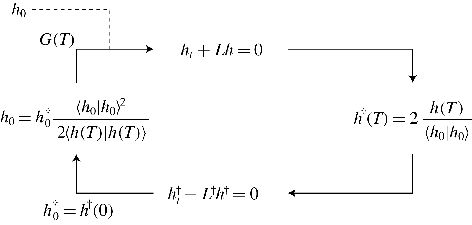
In order to find the optimal initial condition, one starts with an arbitrary initial condition
 $h_{0}$
and integrates the direct problem (4.3) forward in time from
 $t=0$
to the chosen time horizon
 $t=T$
(see appendix C for details of the numerical method). The adjoint (4.9) is then integrated backward in time, starting from the condition (4.8) at
 $t=T$
and using the adjoint operator
 $L^{\dagger }=L^{T}$
. The latter satisfies the property
 $\langle a\mid Lb\rangle =\langle L^{\dagger }a\mid b\rangle$
. The Lagrange multiplier
 $h_{0}^{\dagger }$
is given by (4.10), and the new guess for the optimal initial condition is given by (4.11). This algorithm (see figure 6) is repeated until the gain
 $G(T)$
converges, eventually yielding the optimal initial condition and the optimal gain for a particular time horizon
 $T$
, spanwise wavenumber
 $\unicode[STIX]{x1D6FD}$
, Bond number
 $Bo$
and film aspect ratio
 $\unicode[STIX]{x1D6FF}$
. By repeating the same procedure for successive time horizons
 $T$
, the envelope of the optimal gains for the selected parameters can be found.
Sketch of the iterative procedure to find the optimal gain and initial condition for a given time horizon
 $T$
, spanwise wavenumber
 $\unicode[STIX]{x1D6FD}$
, Bond number
 $Bo$
and film aspect ratio
 $\unicode[STIX]{x1D6FF}$
.

4.4 Results
4.4.1 Influence of the time horizon
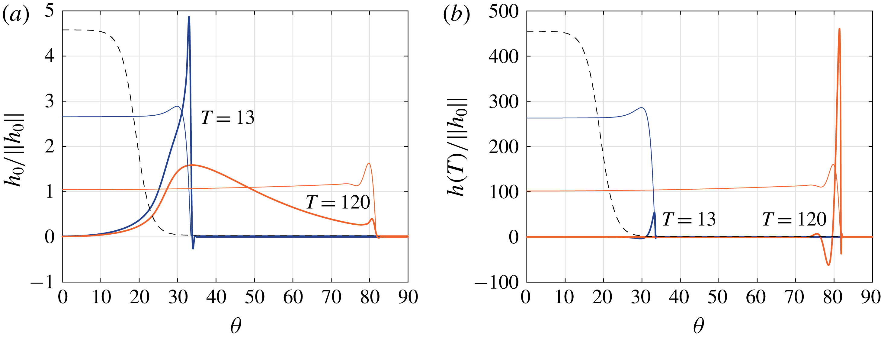
(a) Optimal initial conditions
 $h_{0}$
and (b) optimal responses
 $h(T)$
for the time horizons
 $T=13$
and
 $120$
(thick solid lines), normalized by the initial
 $L_{2}$
-norm of the perturbation
 $\Vert h_{0}\Vert$
. The thin solid lines indicate the base flow profile
 $H$
at the times
 $T$
and the black dashed line are the base flow at
 $t=0$
(in arbitrary units). Here
 $\unicode[STIX]{x1D6FD}=2$
.

As can be seen in figure 7(a), we have found that the optimal initial film perturbation profile depends on the optimization time
 $T$
. At short time horizons the profile mainly consists of a localized perturbation close to the region reached by the ridge of the draining flow at
 $t=T$
. At large time horizons, instead, the profile presents a significant wide-bump perturbation over the entire region swept by the draining-flow ridge. In agreement with the sensitivity of the instability on the detail of the ridge, and thus on the details of the perturbations at the virtual contact line (Bertozzi & Brenner Reference Bertozzi and Brenner1997), the optimal perturbations are found to be mainly located in the precursor-film region (see § 3). Due to the very small thickness of the precursor film, the mobility of the perturbations is almost none. The perturbations flow only after the base flow front has reached their location.
The optimal responses are, on the other hand, located in the inner region of the draining flow (see figure 7 b). Despite the fact that their structure is very similar to the dominant eigenfunction for the flow over an inclined plane (Spaid & Homsy Reference Spaid and Homsy1996), the precise profile of the response changes with time due to the space-dependent forces at play.
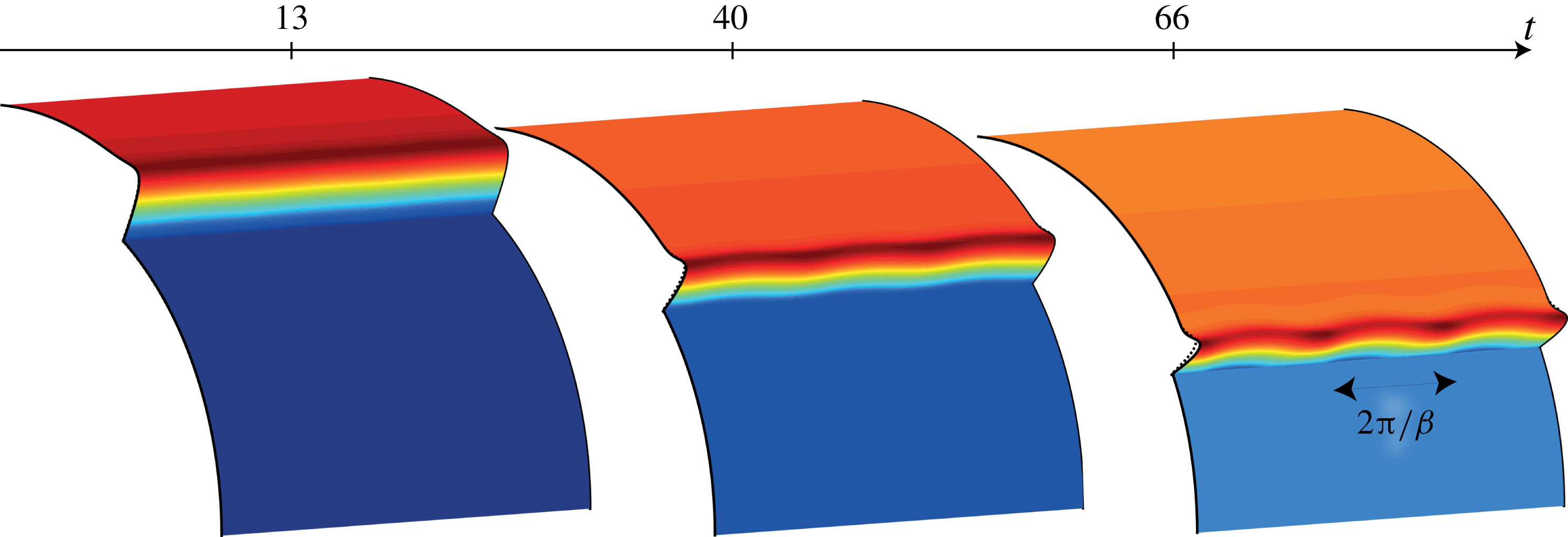
Evolution of the total film thickness
 $\bar{H}=H+\unicode[STIX]{x1D700}h$
starting from the optimal initial condition
 $h_{0}$
for
 $T=120$
at the times
 $t=13$
,
 $40$
and
 $66$
. The dashed lines indicate the base flow profile
 $H$
at the selected times. Here
 $\unicode[STIX]{x1D6FD}=2$
. The perturbations are rescaled by the maximum of the initial condition
 $h_{0}$
for visualization purposes and
 $\unicode[STIX]{x1D700}=10^{-3}$
.

For the sake of clarity, we present in figure 8 the evolution of the total film thickness, i.e. the base draining flow
 $H$
plus the disturbance field
 $h$
given by the optimal initial condition
 $h_{0}$
scaled by an arbitrary
 $\unicode[STIX]{x1D700}=10^{-3}$
. The perturbations induce an increase/decrease in the film thickness at the front (see for instance the total profile at
 $t=66$
), sinusoidally modulated in the spanwise direction with a wavenumber
 $\unicode[STIX]{x1D6FD}$
; see (4.2). If nonlinear effects were considered, thicker regions would eventually flow faster than the thinner ones and fingers would form.
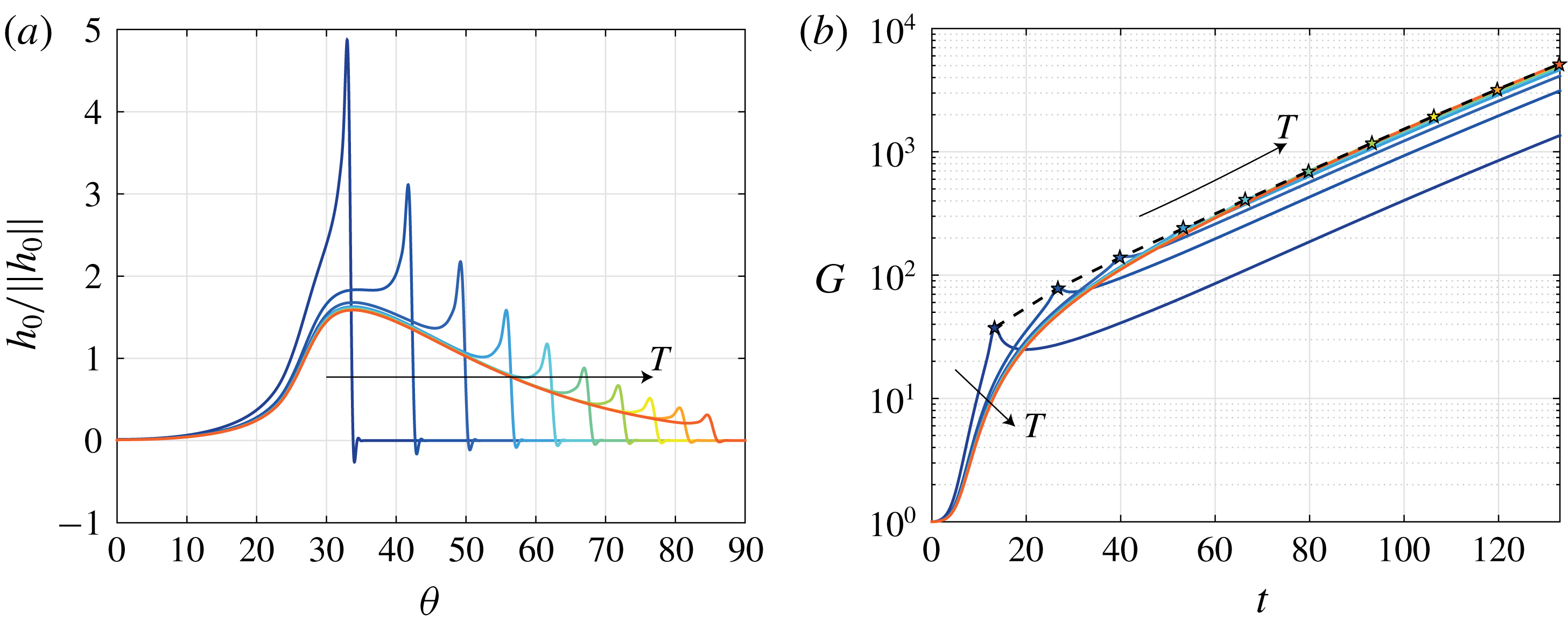
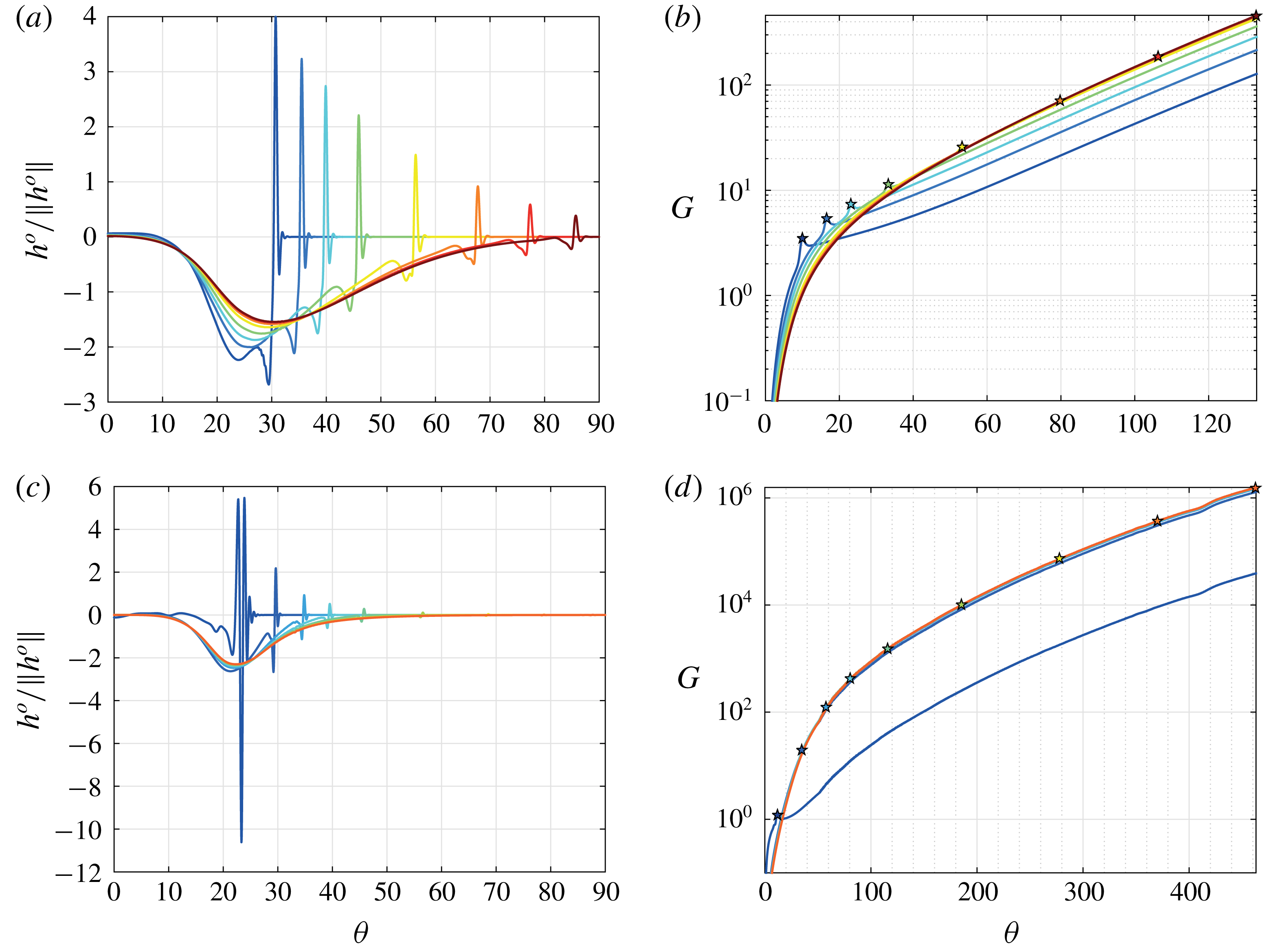
Optimal initial conditions
 $h_{0}$
, normalized by the initial
 $L_{2}$
-norm of the perturbation
 $\Vert h_{0}\Vert$
(a) and gain
 $G$
(b) for the time horizons
 $T=13$
,
 $27$
,
 $40$
,
 $53$
,
 $66$
,
 $80$
,
 $93$
,
 $106$
,
 $120$
and
 $133$
. The stars indicate the optimal gains
 $G_{max}=G(T)$
. The black dashed line corresponds to the envelope of the gains
 $G_{max}$
. Here
 $\unicode[STIX]{x1D6FD}=2$
.

When looking at the gain evolutions for several optimal initial conditions, it can be observed that the gains increase with time also after the time horizon
 $T$
(see figure 9). The rationale for this is the fact that the ridge continues advancing and remains locally unstable (Huerre & Rossi Reference Huerre and Rossi1998) for the considered wavenumber. Furthermore, the time-dependent slope of the gain evolution, which would correspond to an instantaneous growth rate, indicates that the problem is not stationary so that an eigenvalue decomposition cannot be employed. In the linear regime, a flow on an inclined plane would develop an exponentially growing instability at the front (Spaid & Homsy Reference Spaid and Homsy1996).
The structure of the optimal initial conditions progressively changes from a localized perturbation at the front for small
 $T$
to a wide-bump perturbation for large
 $T$
(see figure 9
a). In contrast to the optimal initial perturbations at short times, the wide-bump structure of the optimal perturbations for large time horizons induces a large gain over a longer time interval. In fact, the ridge of the draining flow is continuously perturbed by the initial optimal disturbance located in the precursor film over a wide polar range. Thereby, the optimal perturbation for large time horizons is less specific to a precise time. The optimal initial conditions for large time horizons become more and more similar, sharing the same wide-bump structure, with the thickest region at the same polar angle.
By interpolating the optimal gains
 $G_{max}=G(T)$
one can define the envelope of the optimal gains. Due to the previous observation, the envelope coincides with the evolutions of the gains for the late times horizons.
4.4.2 Optimal spanwise wavenumber
Thus far the spanwise wavenumber
 $\unicode[STIX]{x1D6FD}=2$
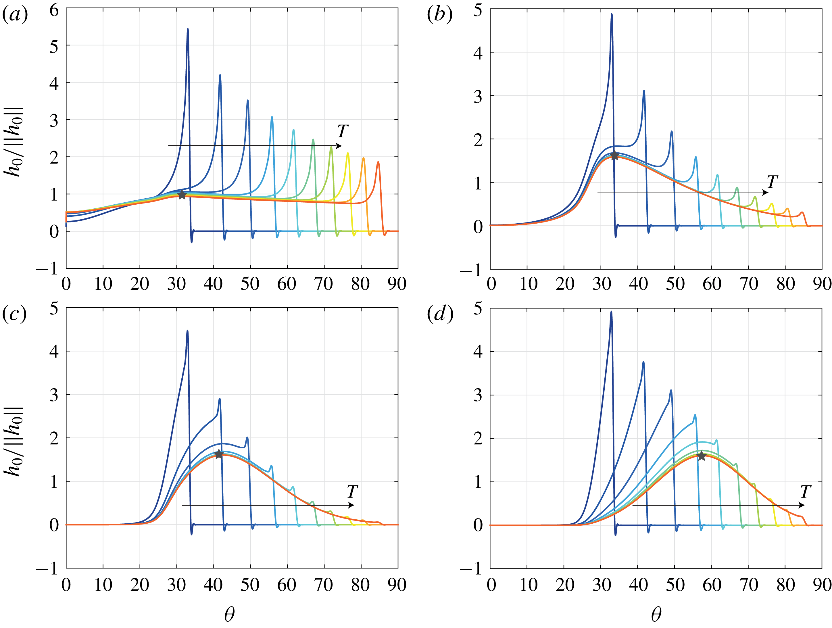
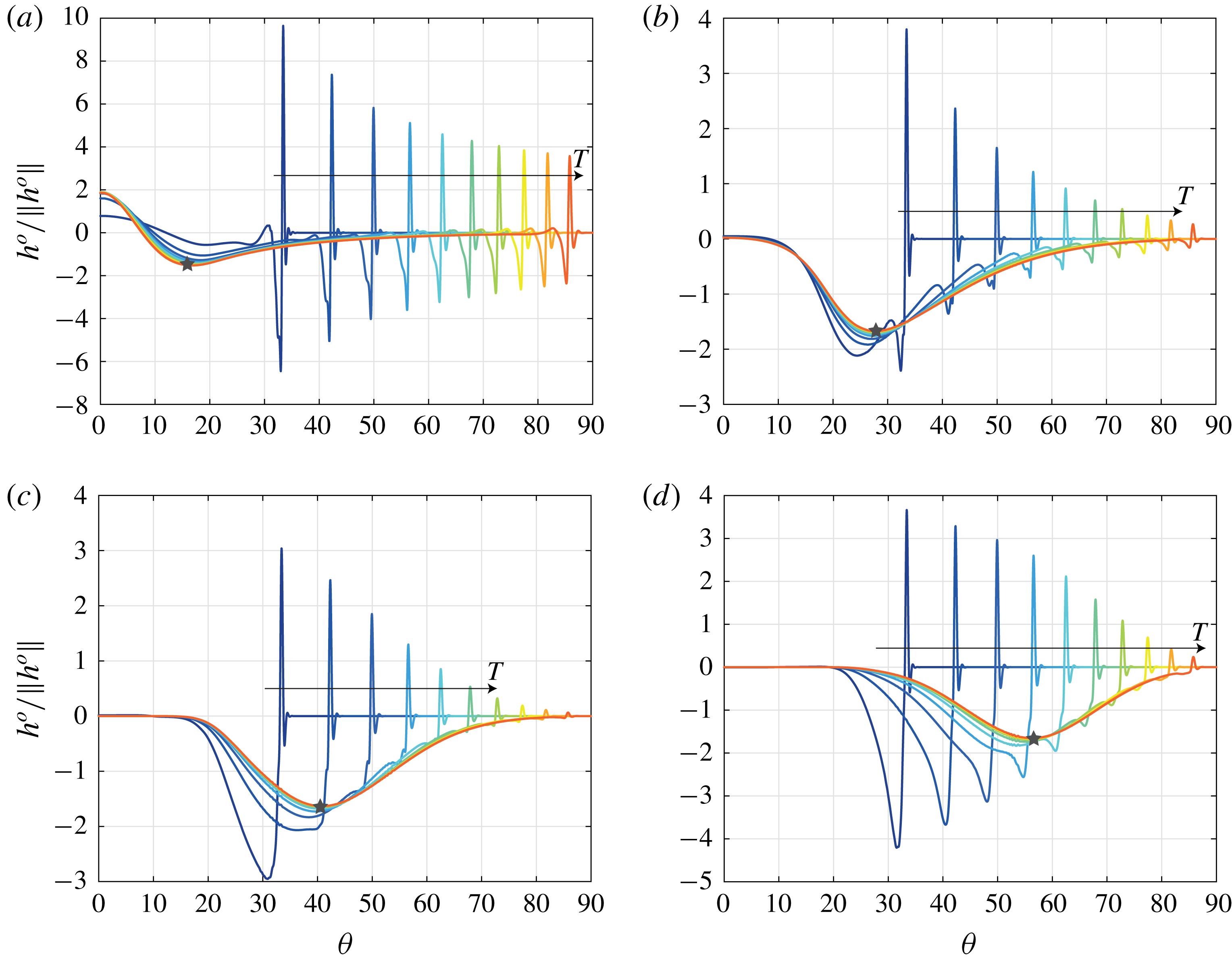
has been considered. As can be seen in figure 10, most of the optimal initial conditions for different spanwise wavenumbers
 $\unicode[STIX]{x1D6FD}$
also present a localized perturbation for small
 $T$
and a wide-bump perturbation for large time horizons.
Optimal initial conditions
 $h_{0}$
, normalized by the initial
 $L_{2}$
-norm of the perturbation
 $\Vert h_{0}\Vert$
, for the time horizons
 $T=13$
,
 $27$
,
 $40$
,
 $53$
,
 $66$
,
 $80$
,
 $93$
,
 $106$
,
 $120$
and
 $133$
for
 $\unicode[STIX]{x1D6FD}=$
(a) 0.5, (b) 2, (c) 4 and (d) 6. The stars indicate the thickest location of the wide-bump perturbation.

The maximum of the wide-bump perturbation is located at a polar location which increases with
 $\unicode[STIX]{x1D6FD}$
(see stars in figure 10). This result can be understood by recalling the dependence of the most amplified spanwise wavenumber on the length of the capillary ridge
 $\ell$
for the flow over an inclined plane:
 $\unicode[STIX]{x1D6FD}\sim 1/\ell$
(Troian et al.
Reference Troian, Herbolzheimer, Safran and Joanny1989; Spaid & Homsy Reference Spaid and Homsy1996). For the flow over a cylinder, we have seen in (3.8) that
 $\ell$
decreases as
 $\unicode[STIX]{x1D703}_{N}$
increases in the gravity–capillary regime (see table 1). Hence, when the advancing front reaches larger polar angles, larger spanwise wavenumber will be more effective. For large spanwise wavenumbers, the optimal perturbation at small time horizons
 $T$
, i.e. for small polar angles, corresponds to a localized perturbation at the front, since perturbing a larger region, which penalizes the gain, is not effective.
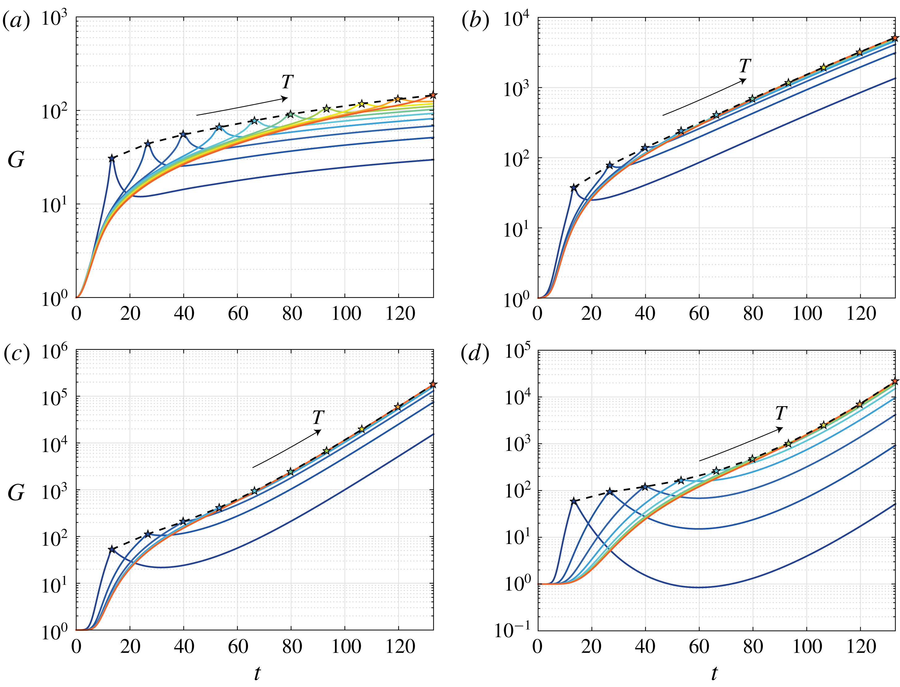
Gain
 $G$
for the time horizons
 $T=13$
,
 $27$
,
 $40$
,
 $53$
,
 $66$
,
 $80$
,
 $93$
,
 $106$
,
 $120$
and
 $133$
for
 $\unicode[STIX]{x1D6FD}=$
(a) 0.5, (b) 2, (c) 4 and (d) 6. The stars indicate the optimal gains
 $G_{max}=G(T)$
. The black dashed lines correspond to the envelope of the gains
 $G_{max}$
.

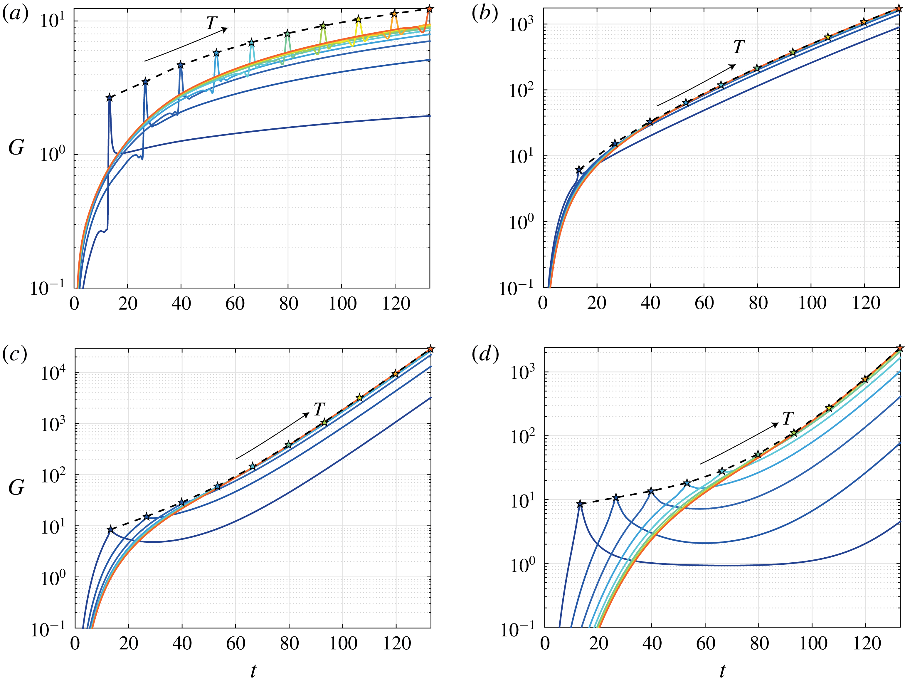
In view of the dependence of the wide-bump location on the spanwise wavenumber and the different gain evolution induced by the localized and wide-bump perturbations (see figure 9), the achievable gain also depends on the spanwise wavenumber
 $\unicode[STIX]{x1D6FD}$
(see figure 11). We have found that for small and large
 $\unicode[STIX]{x1D6FD}$
, typically
 $\unicode[STIX]{x1D6FD}<2$
and
 $\unicode[STIX]{x1D6FD}>7$
, the wide-bump perturbation is never optimal in the range
 $\unicode[STIX]{x1D703}\in [0,\unicode[STIX]{x03C0}/2]$
. Thus, the localized initial condition dominates and the gain evolutions present a clear peak for times close to the time horizons. Conversely, when the optimal initial conditions present a similar wide-bump structure, their gain evolutions are closer and reach much larger values.
Envelopes
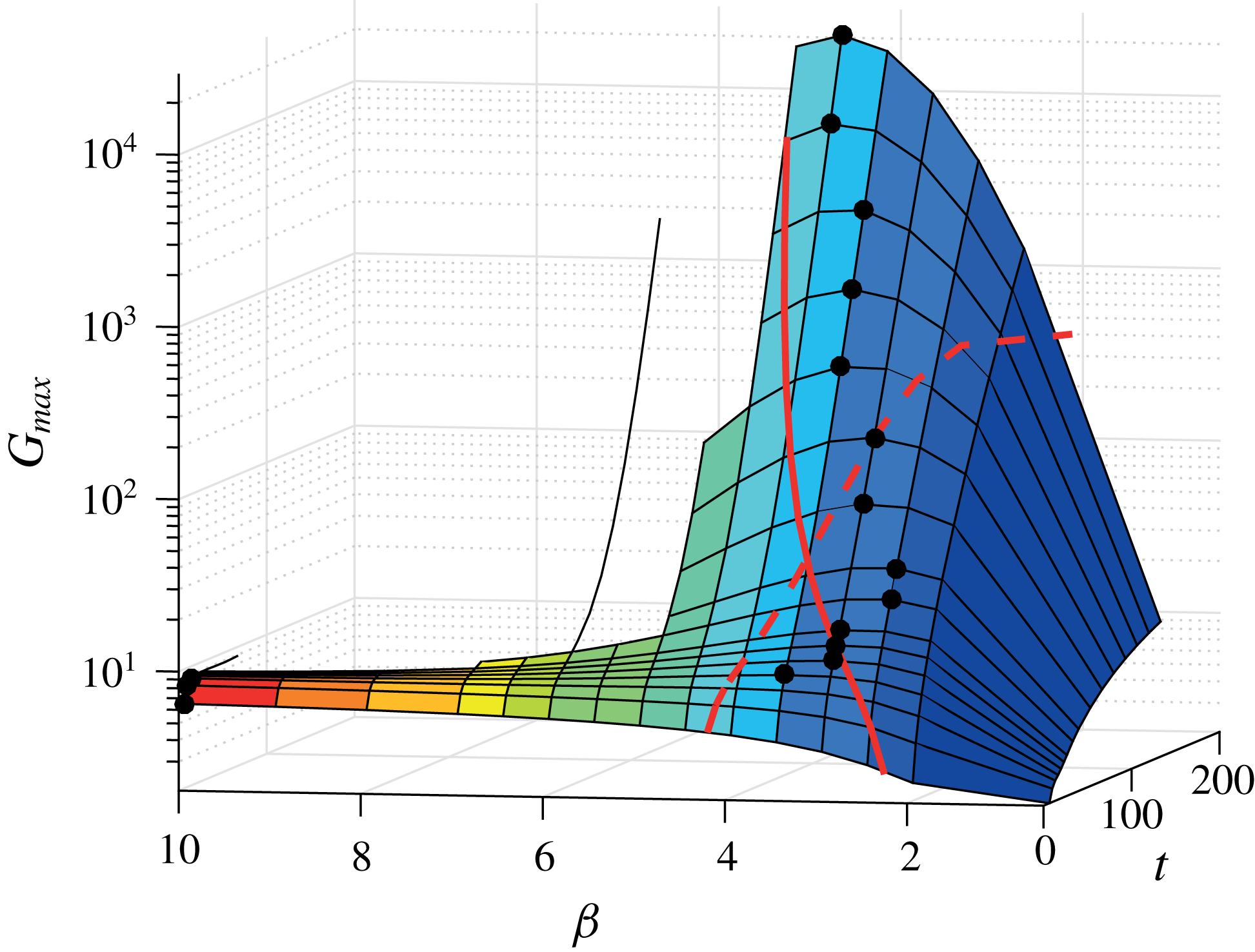
 $G_{max}(\unicode[STIX]{x1D6FD},t)$
for the gain evolutions induced by initial film-thickness perturbations for
 $\unicode[STIX]{x1D6FD}=0.5$
,
 $1$
,
 $2$
,
 $2.5$
,
 $3$
,
 $3.5$
,
 $4$
,
 $4.5$
,
 $5$
,
 $5.5$
,
 $6$
,
 $6.5$
and
 $10$
. The largest optimal gains obtained by the transient growth analysis, and the corresponding optimal wavenumbers
 $\unicode[STIX]{x1D6FD}$
, at every considered time, are indicated by the black symbols. The optimal wavenumbers given by inclined-plane theory with
 $\unicode[STIX]{x1D6FD}=0.5/\ell _{c}$
(red dashed line) and
 $\unicode[STIX]{x1D6FD}=0.5/\ell$
(red solid line) are also represented.

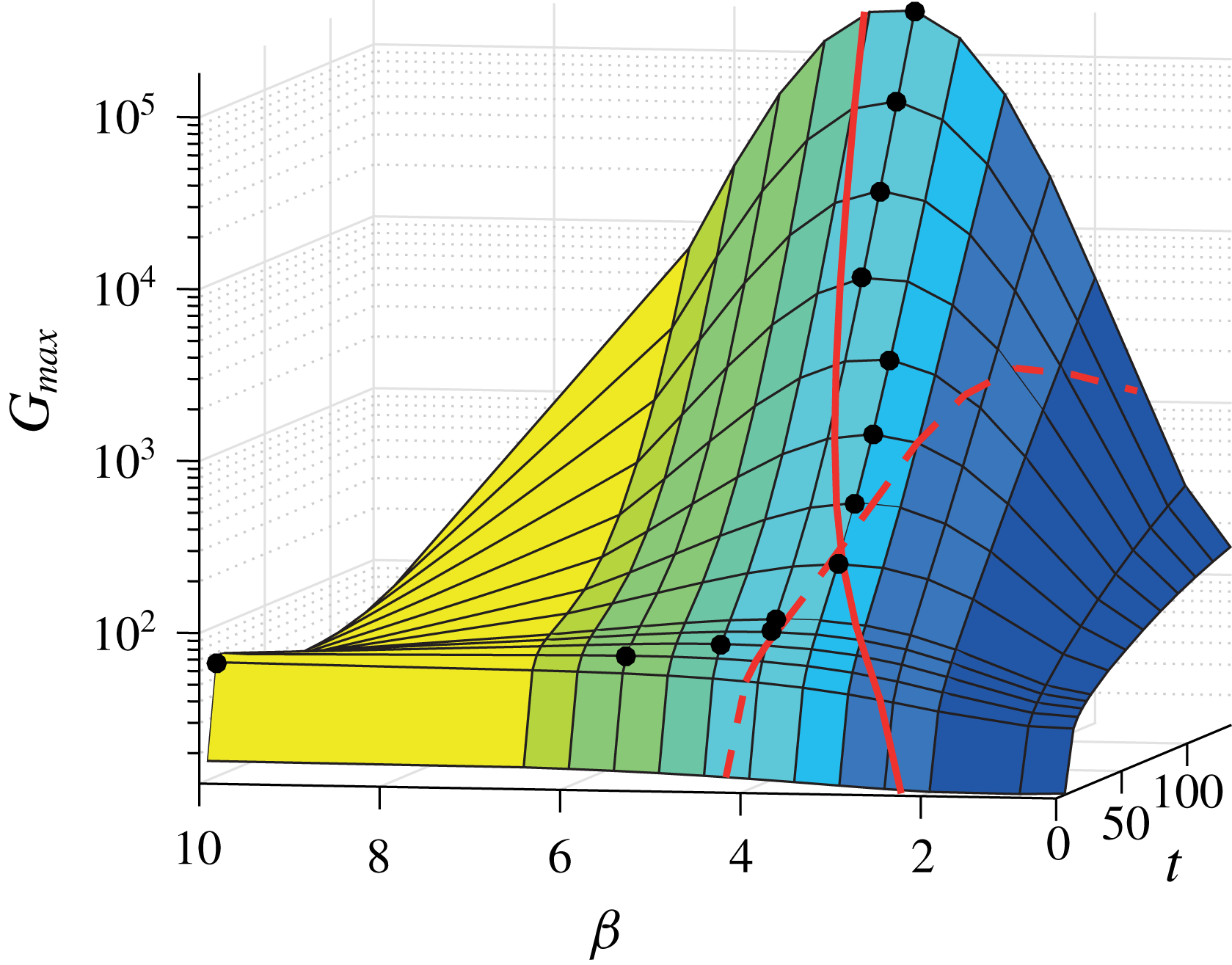
The spanwise-wavenumber dependence of the gain is clearly visible in figure 12, where all the computed gain envelopes are shown. The gain at the smallest considered time horizon increases monotonically with
 $\unicode[STIX]{x1D6FD}$
for
 $0<\unicode[STIX]{x1D6FD}\leqslant 10$
, but its value remains small. On the contrary, the gain for large time horizons is not monotonic with
 $\unicode[STIX]{x1D6FD}$
, indicating that an optimal
 $\unicode[STIX]{x1D6FD}$
exists. Strikingly, we have found that the optimal initial condition which is the least affected by the time horizon, and thus is the most universal (see for example figure 10
c and figure 11
c), yields the largest gain at large times.
The optimal spanwise wavenumber as a function of time (see symbols in figure 12) can be again qualitatively rationalized with the help of the relation
 $\unicode[STIX]{x1D6FD}=c/\ell$
, obtained by the linear stability analysis for the flow over an inclined plane.
The precise value of the proportionality coefficient
 $c$
depends on the model for the moving contact line (Spaid & Homsy Reference Spaid and Homsy1996). However, its value is found to be always around
 $0.5$
(Troian et al.
Reference Troian, Herbolzheimer, Safran and Joanny1989; Spaid & Homsy Reference Spaid and Homsy1996). At short times, typically
 $t\lesssim 40$
, the optimal wavenumber found by the optimal transient growth analysis decreases with time, from
 $\unicode[STIX]{x1D6FD}=10$
to
 $3.5$
. During this time, the base flow strongly evolves from the particular initial condition to the well-developed draining flow (see for instance figure 4), and the characteristic length of the ridge is
 $\ell _{c}$
, given by (3.7). Since
 $\ell _{c}$
increases with time, the optimal wavenumber
 $\unicode[STIX]{x1D6FD}=0.5/\ell _{c}$
decreases (see dashed line in figure 12). However, for
 $t\gtrsim 40$
, the base drainage solution reaches the well-developed state where the characteristic length of the ridge is given by
 $\ell$
, equation (3.8). The optimal wavenumber
 $\unicode[STIX]{x1D6FD}=0.5/\ell$
increases with time since
 $\ell$
decreases (see solid line in figure 12). For the late time limit,
 $t\gg \unicode[STIX]{x1D70F}_{i}$
,
 $\unicode[STIX]{x1D6FD}\sim 0.5(2Bo\,t/3)^{1/3}$
(see table 1). The crossover time for the ridge length from
 $\ell _{c}$
to
 $\ell$
was found to be
 $44$
, in agreement with the change in regime for the optimal wavenumber
 $\unicode[STIX]{x1D6FD}$
.
However, the precise value for the optimal wavenumber found by the optimal transient growth for large times is smaller than that predicted by the local inclined-plane theory (see solid line in figure 12). The reason lies in the transient behaviour of the draining flow. In fact, the instability inherits from the past history, and thus from the growth in a region with a smaller inclination, which promotes smaller wavenumbers. Furthermore, the linear stability analysis of the flow over an inclined plane also fails at quantitatively predicting the optimal wavelength at very short times, where the transient dynamics is essential. Thus, a transient growth analysis such as the one performed in this work is crucial for predicting the optimal spanwise wavenumber and the optimal gains for all times.
In their experiment, Takagi & Huppert (Reference Takagi and Huppert2010) observed the formation of fingers between
 $t^{\ast }=0.7~\text{s}$
and
 $t^{\ast }=1.5~\text{s}$
with a wavelength of about
 $5~\text{cm}$
. Given their cross-sectional area of fluid
 $A=5.2~\text{cm}^{2}$
, kinematic viscosity
 $\unicode[STIX]{x1D708}=5.1~\text{cm}^{2}~\text{s}^{-1}$
and cylinder of radius
 $R=15~\text{cm}$
, the characteristic length is
 $L=\sqrt{A}=2.3~\text{cm}$
and the characteristic time is
 $\unicode[STIX]{x1D70F}_{d}=0.015~\text{s}$
. The dimensionless fingers-formation time is in the range
 $t=47{-}100$
, which corresponds to an optimal wavenumber
 $\unicode[STIX]{x1D6FD}$
between 3.5 and 4 (see figure 12). Thus, our analysis based on the growth of initial film-thickness perturbations predicts a fingering wavelength in the range 3.6–4.1 cm, which is slightly smaller than the observed experimental value. However, it has to be stressed that in the experiment of Takagi & Huppert (Reference Takagi and Huppert2010) the initial conditions are slightly different and only two fingers form due to the strong lateral confinement induced by the finite length of the cylinder. Another possible explanation for the experimentally observed fingering wavelength of Takagi & Huppert (Reference Takagi and Huppert2010) follows in § 5.5.2.
The physical outcome of this section is that, depending on the amplitude of the film perturbations, a different spanwise wavenumber will be selected. If the perturbations are strong, a small gain will be sufficient and fingers with a large wavenumber will form at short times. Nevertheless, since the differences in gains at short times are not significant, the distribution of promoted wavelengths is larger, as already observed by Silvi & Dussan (Reference Silvi and Dussan1985) for low plate-inclination angles. On the other hand, if the perturbation amplitude is small, a large amplification will be necessary and fingers will only form at late times with a smaller wavenumber.
To conclude, from the optimization of the initial conditions over a smooth surface we have learned that an optimal wavenumber exists and that, for late times, it corresponds to the least horizon-dependent optimal initial conditions, allowing for an optimal growth over a longer time. Note that at later times,
 $t>t_{f}=133$
, the ridge is on the lower part of the cylinder and is asymptotically unstable to the Rayleigh–Taylor instability (Indeikina et al.
Reference Indeikina, Veretennikov and Chang1997; Takagi & Huppert Reference Takagi and Huppert2010).
Since the perturbation in the thin-film region is stationary, one is tempted to ask the question as to whether or not the perturbation of the precursor film thickness can be also attributed to a perturbation in the substrate. This is the subject of § 5.
5 Optimal substrate perturbations for an initially unperturbed film
5.1 Lubrication equation with a perturbed substrate
The substrate has been, so far, considered as perfectly cylindrical. However, it is also possible to consider topographical perturbations of the substrate, denoted as
 $\bar{H}^{o\ast }$
, that perturb the fluid. The free surface is then defined by
 $F=r^{\ast }-(R+\bar{H}^{\ast }+\bar{H}^{o\ast })=0$
. Since the derivation of a lubrication equation for this configuration is more involved, we will restrict our analysis to a particular case. First, we assume that the substrate perturbations are infinitesimally small such that the base flow
 $H$
discussed in § 3 is unaffected, and remains therefore invariant in the axial direction. Second, since a linear problem is eventually derived for the optimal substrate perturbations analysis, only linear terms in the substrate-topography perturbations are kept for consideration. The full derivation of the lubrication equation for this case can be found in appendix B. In dimensionless form it reads
 $$\begin{eqnarray}\displaystyle & & \displaystyle \bar{H}_{t}+\frac{1}{3}\left\{\bar{H}^{3}\left[\frac{\unicode[STIX]{x1D6FF}^{2}}{Bo}\bar{\unicode[STIX]{x1D705}}_{\unicode[STIX]{x1D703}}-\unicode[STIX]{x1D6FF}\cos \unicode[STIX]{x1D703}(\bar{H}_{\unicode[STIX]{x1D703}}+\bar{H}_{\unicode[STIX]{x1D703}}^{o})+\sin \unicode[STIX]{x1D703}\right]\right\}_{\unicode[STIX]{x1D703}}\nonumber\\ \displaystyle & & \displaystyle \quad +\,\frac{1}{3\unicode[STIX]{x1D6FF}}\left\{\bar{H}^{3}\left[\frac{\unicode[STIX]{x1D6FF}}{Bo}\bar{\unicode[STIX]{x1D705}}_{z}-\cos \unicode[STIX]{x1D703}(\bar{H}_{z}+\bar{H}_{z}^{o})-\unicode[STIX]{x1D6FF}\sin \unicode[STIX]{x1D703}\bar{H}\bar{H}_{\unicode[STIX]{x1D703}z}^{o}\right]\right\}_{z}=0.\end{eqnarray}$$
The curvature is given by
 $\bar{\unicode[STIX]{x1D705}}=-\unicode[STIX]{x1D735}\boldsymbol{\cdot }\boldsymbol{n}$
with
 $\boldsymbol{n}$
the normal vector to the free surface (see expression (B 1)). It therefore includes contributions from the surface topography, as seen in expression (B 11) where only linear contributions in
 $\bar{H}^{o}$
have been kept in anticipation to the subsequent linearization (§§ 5.2 and 5.3). The curvature is eventually truncated at the second order in
 $\unicode[STIX]{x1D6FF}$
to keep only the leading-order terms.
5.2 Free-surface-elevation decomposition
When the substrate is perturbed, i.e.
 $\bar{H}^{o}\neq 0$
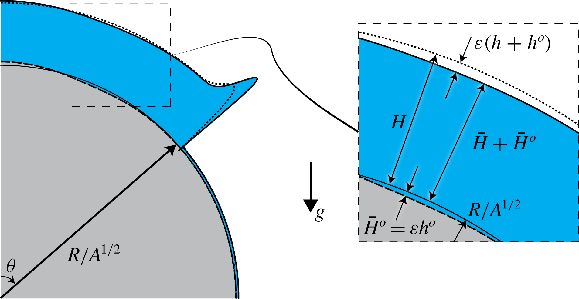
, the free surface of the film is located at a distance
 $\bar{H}+\bar{H}^{o}$
from the originally smooth cylindrical substrate. Here, we consider only small time-independent substrate perturbations of order
 $\unicode[STIX]{x1D700}\ll 1$
:
 $\bar{H}^{o}=\unicode[STIX]{x1D700}{\hat{h}}^{o}$
. Hence, the elevation of the film free surface can be decomposed as (see figure 13)
 $$\begin{eqnarray}\displaystyle \bar{H}(\unicode[STIX]{x1D703},z,t)+\bar{H}^{o}(\unicode[STIX]{x1D703},z)=\underbrace{H(\unicode[STIX]{x1D703},t)}_{drainage\;solution}+\;\unicode[STIX]{x1D700}\left[\underbrace{{\hat{h}}(\unicode[STIX]{x1D703},z,t)}_{\;film\;perturbation}+\underbrace{{\hat{h}}^{o}(\unicode[STIX]{x1D703},z)}_{substrate\;perturbation}\right],\quad \unicode[STIX]{x1D700}\ll 1.\quad & & \displaystyle\end{eqnarray}$$
Decomposition of the free-surface elevation
 $\bar{H}+\bar{H}^{o}$
starting from the smooth cylindrical substrate into draining solution
 $H$
and first-order perturbations
 $\unicode[STIX]{x1D700}(h+h^{o})$
for the optimal transient growth over a perturbed substrate with an initially uniform film. It is important to stress that the liquid thickness is only
 $\bar{H}=H+\unicode[STIX]{x1D700}h$
, whereas
 $\bar{H}^{o}=\unicode[STIX]{x1D700}h^{o}$
is the substrate-topography perturbation. The axial dependence as in figure 5 is not repeated here.

As for the study of the optimal initial conditions of § 4, given the invariance of the base state in the
 $z$
-direction, we consider periodic perturbations in the transverse direction:
 $$\begin{eqnarray}\displaystyle & \displaystyle {\hat{h}}(\unicode[STIX]{x1D703},z,t)=h(\unicode[STIX]{x1D703},t)\exp (\text{i}\unicode[STIX]{x1D6FD}z)+\text{c.c.}, & \displaystyle\end{eqnarray}$$
 $$\begin{eqnarray}\displaystyle & \displaystyle {\hat{h}}^{o}(\unicode[STIX]{x1D703},z)=h^{o}(\unicode[STIX]{x1D703})\exp (\text{i}\unicode[STIX]{x1D6FD}z)+\text{c.c.}, & \displaystyle\end{eqnarray}$$
where
 $\unicode[STIX]{x1D6FD}\in \mathbb{R}$
is the spanwise wavenumber. It is important not to confuse
 $h_{0}$
, the initial condition of the perturbation, with
 $h^{o}$
, the substrate profile. The one-dimensional perturbations
 $h^{o}(\unicode[STIX]{x1D703})$
have to be optimized for a given spanwise wavenumber
 $\unicode[STIX]{x1D6FD}$
.
5.3 Linear disturbance equation
The governing equation for the first-order disturbances is obtained by entering the film-thickness decomposition (5.2) together with (5.3) and (5.4) into the nonlinear lubrication (5.1) and considering terms at order
 $\unicode[STIX]{x1D700}$
:
 $$\begin{eqnarray}\displaystyle h_{t}+L(H,\unicode[STIX]{x1D6FD},Bo,\unicode[STIX]{x1D6FF})h=-L^{o}(H,\unicode[STIX]{x1D6FD},Bo,\unicode[STIX]{x1D6FF})h^{o}. & & \displaystyle\end{eqnarray}$$
The linear operators
 $L(H,\unicode[STIX]{x1D6FD},Bo,\unicode[STIX]{x1D6FF})$
, which is the same as in § 4, and
 $L^{o}(H,\unicode[STIX]{x1D6FD},Bo,\unicode[STIX]{x1D6FF})$
are a function of the drainage solution, the spanwise wavenumber, the Bond number and the film aspect ratio (see appendix A for their expressions). Thus, the linear operators are space dependent and are not autonomous.
As expected, the perturbation of the substrate topography results in the appearance of a time-dependent – through
 $H(\unicode[STIX]{x1D703},t)$
– forcing term:
 $L^{o}(H,\unicode[STIX]{x1D6FD},Bo,\unicode[STIX]{x1D6FF})h^{o}$
. Note that a change of variable in order to homogenize (5.5), making the optimal substrate and the optimal initial condition problems mathematically similar (the state variable being only the difference
 $h-h^{o}$
), was found not to be possible due to the time dependency of the forcing term.
5.4 Optimization method
We will now derive the equations leading to the optimization algorithm for the substrate-topography perturbations. The gain to be optimized at a time horizon
 $T$
is defined as the ratio of the film disturbance energy
 $E(T)$
and the substrate disturbance energy
 $E^{o}=\langle h^{o}\mid h^{o}\rangle /2$
:
 $$\begin{eqnarray}\displaystyle G(T)=\frac{E(T)}{E^{o}}=\frac{\langle h(T)\mid h(T)\rangle }{\langle h^{o}\mid h^{o}\rangle }. & & \displaystyle\end{eqnarray}$$
The choice of the gain (5.6) requires a vanishing initial free-surface disturbance,
 $h_{0}=0$
, otherwise the algorithm will bring
 $h^{o}$
to zero naturally, leading to an infinite gain as soon as
 $h(T)$
is a non-zero number. Perturbing the substrate – the forcing term in the state (5.5) – is the only way to perturb the base flow. This choice also has a practical relevance since it is sufficient to let the base flow evolve on the perturbed substrate, without having to experimentally impose an initial condition for the fluid’s perturbation. Another possible choice for the gain is
 $\langle h(T)\mid h(T)\rangle -\unicode[STIX]{x1D712}\langle h^{o}\mid h^{o}\rangle$
. Such a choice would relax the condition
 $h_{0}=0$
, to the price of depending on the value of the penalization coefficient
 $\unicode[STIX]{x1D712}$
. We have therefore not retained this gain definition hereafter.
The augmented Lagrangian reads
 $$\begin{eqnarray}\displaystyle {\mathcal{L}}(h,h^{\dagger },h^{o};T)=\underbrace{G(T)}_{gain}-\underbrace{\int _{0}^{T}\langle h^{\dagger }\mid h_{t}+Lh+L^{o}h^{o}\rangle \,\text{d}t}_{enforcing\;governing\;equation}. & & \displaystyle\end{eqnarray}$$
By proceeding in the same manner as for the derivation of the algorithm for the optimal initial condition of § 4.3, the adjoint equations for the Lagrange multiplier
 $h^{\dagger }$
are given by setting to zero the first variations of
 ${\mathcal{L}}$
with respect to any variation
 $\unicode[STIX]{x1D6FF}h$
:
 $$\begin{eqnarray}\displaystyle \displaystyle \left\langle \frac{\unicode[STIX]{x2202}{\mathcal{L}}}{\unicode[STIX]{x2202}h}\biggm\vert\unicode[STIX]{x1D6FF}h\right\rangle =0,\quad \forall \unicode[STIX]{x1D6FF}h\Leftrightarrow & & \displaystyle \!\!\!\!h^{\dagger }(T)=2\frac{h(T)}{\langle h^{o}|h^{o}\rangle },\end{eqnarray}$$
 $$\begin{eqnarray}\displaystyle & & \displaystyle \displaystyle \!\!\!\!h_{t}^{\dagger }-L^{\dagger }h^{\dagger }=0,\quad t\in [0,T].\end{eqnarray}$$
The optimality condition for the substrate perturbation is obtained by imposing a zero Fréchet derivative of
 ${\mathcal{L}}$
with respect to
 $h^{o}$
(see derivation in appendix D):
 $$\begin{eqnarray}\displaystyle \left\langle \frac{\unicode[STIX]{x2202}{\mathcal{L}}}{\unicode[STIX]{x2202}h^{o}}\biggm\vert\unicode[STIX]{x1D6FF}h^{o}\right\rangle =0,\quad \forall \unicode[STIX]{x1D6FF}h^{o}\Leftrightarrow \frac{h^{o}}{\langle h^{o}|h^{o}\rangle ^{2}}=\frac{1}{-2\langle h(T)\mid h(T)\rangle }\int _{0}^{T}L^{o\dagger }h^{\dagger }\,\text{d}t. & & \displaystyle\end{eqnarray}$$
By deriving the augmented Lagrangian with respect to the multiplier one retrieves the constraint. Both liquid film direct and adjoint perturbations, as well as the substrate perturbations satisfy the following boundary conditions:
 $h_{\unicode[STIX]{x1D703}}(0)=h_{\unicode[STIX]{x1D703}\unicode[STIX]{x1D703}}(0)=0$
,
 $h_{\unicode[STIX]{x1D703}}^{\dagger }(0)=h_{\unicode[STIX]{x1D703}\unicode[STIX]{x1D703}}^{\dagger }(0)=0$
and
 $h_{\unicode[STIX]{x1D703}}^{o}(0)=h_{\unicode[STIX]{x1D703}\unicode[STIX]{x1D703}}^{o}(0)=0$
, and
 $h(\unicode[STIX]{x03C0}/2)=h_{\unicode[STIX]{x1D703}}(\unicode[STIX]{x03C0}/2)=0$
,
 $h^{\dagger }(\unicode[STIX]{x03C0}/2)=h_{\unicode[STIX]{x1D703}}^{\dagger }(\unicode[STIX]{x03C0}/2)=0$
and
 $h^{o}(\unicode[STIX]{x03C0}/2)=h_{\unicode[STIX]{x1D703}}^{o}(\unicode[STIX]{x03C0}/2)=0$
.
In order to find the optimal substrate, one starts with an arbitrary substrate profile
 $h^{o}$
and integrates the direct problem (5.5) from
 $t=0$
to the chosen time horizon
 $t=T$
, with
 $h_{0}=0$
(see appendix C for details of the numerical method). Equation (5.8) gives the initial condition for the adjoint field, which is then integrated backward in time using the adjoint (5.9) from
 $t=T$
to
 $t=0$
. The new guess for the optimal substrate can be found with the help of (5.10). First, the new guess is approximated by
 $$\begin{eqnarray}\displaystyle \tilde{h}^{o}=\frac{1}{-2\langle h(T)\mid h(T)\rangle }\int _{0}^{T}L^{o\dagger }h^{\dagger }\,\text{d}t, & & \displaystyle\end{eqnarray}$$
which is then normalized by
 $\langle \tilde{h}^{o}|\tilde{h}^{o}\rangle ^{2}$
according to equation (5.10) to get
 $h^{o}$
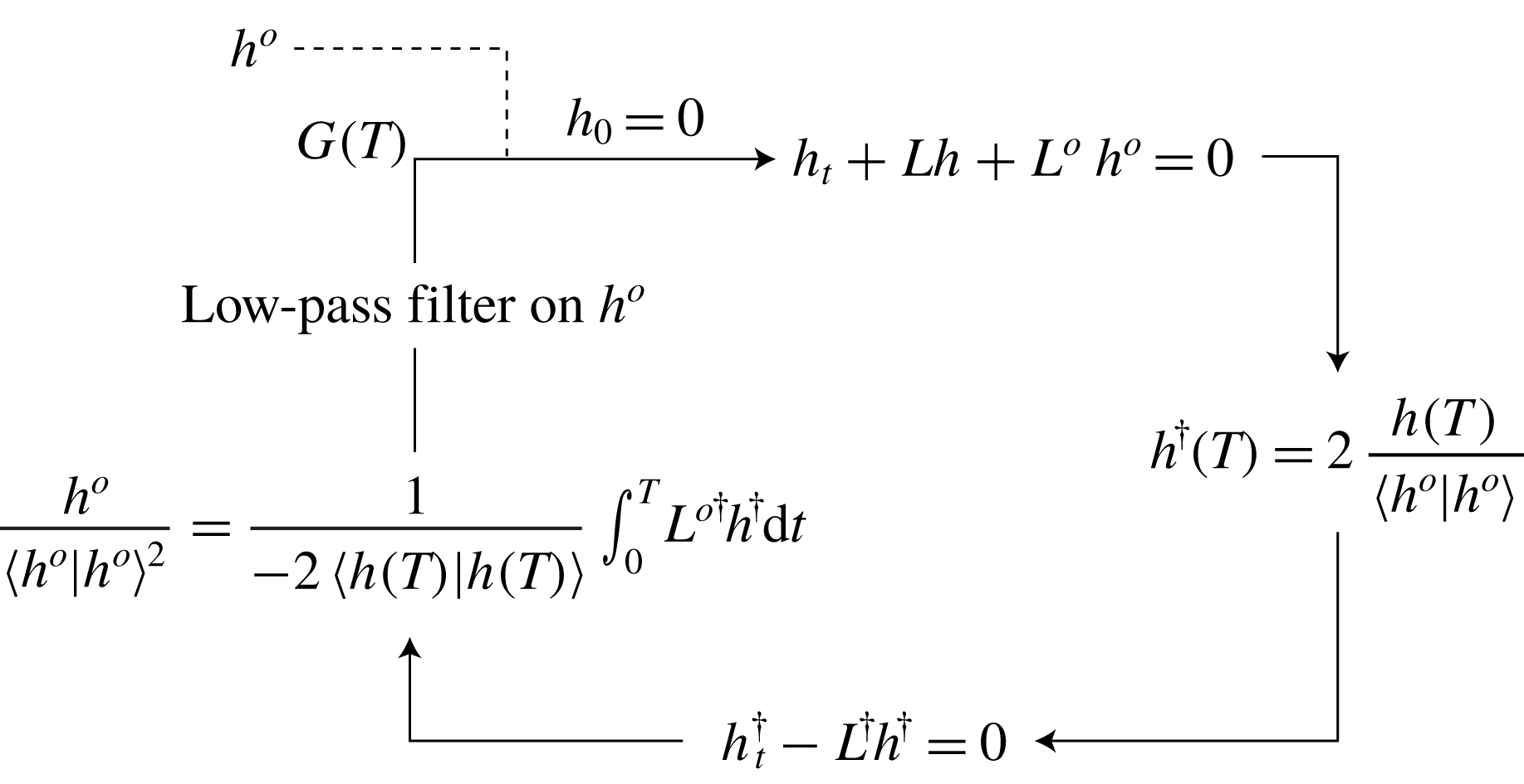
. Second, a low-pass filter is applied to
 $h^{o}$
, whose meaning is explained in the following. The algorithm (see figure 14) is repeated until the gain
 $G(T)$
converges. The optimal substrate as well as the optimal gain for the time horizon
 $T$
, the wavenumber
 $\unicode[STIX]{x1D6FD}$
, the Bond number
 $Bo$
and the film aspect ratio
 $\unicode[STIX]{x1D6FF}$
are obtained. The envelope of the optimal gains for the selected parameters can be found by repeating the procedure for different time horizons
 $T$
.
Sketch of the iterative procedure to find the optimal gain and substrate perturbation for a given time horizon
 $T$
, spanwise wavenumber
 $\unicode[STIX]{x1D6FD}$
, Bond number
 $Bo$
and film aspect ratio
 $\unicode[STIX]{x1D6FF}$
.

The necessity of a low-pass filter for the optimal substrate perturbation can be argued on the grounds of both numerical and physical reasons. In fact, we have found that the optimal substrate after an iteration, before filtering, presents high-frequency perturbations. The latter would result in very large oscillating derivatives in the linear operators
 $L$
and
 $L^{o}$
, compromising therefore the numerical stability. This point is even more dramatic since derivatives up to the fourth order have to be computed. Note that no filter is necessary for the study of § 4 since the optimal initial conditions are regularized by surface-tension effects. The high-frequency perturbations of the optimal substrate perturbations for a given time horizon
 $T$
are situated in the region close to the front location reached by the draining flow at
 $t=T$
. In fact, as already demonstrated by Bertozzi & Brenner (Reference Bertozzi and Brenner1997), the roughness of the substrate at the contact line is an effective amplifier of film perturbations. It is therefore not surprising that the optimal substrate found by the algorithm presents such a rough pattern. However, as will become clear in the following, these localized high-frequency perturbations of the substrate, which dominate at short time horizons
 $T$
, are not the most efficient perturbations. Other perturbations at larger times
 $T$
being of much larger characteristic size and therefore insensitive to the low-pass filter are even more effective. Furthermore, our numerical discretization does not allow for describing a realistic high-frequency random roughness distribution. Therefore, a low-pass filter is applied to smooth out these perturbations (see appendix C for details) and to only consider low-frequency perturbations, which can be resolved accurately. The filter can also be pragmatically justified by noting that, in practice, one can only fabricate an optimal perturbed substrate for experiments with a relatively large characteristic size. The smoothed-out high-frequency perturbations would naturally correspond to the intrinsic roughness of the material surface.
5.5 Results
5.5.1 Influence of the time horizon
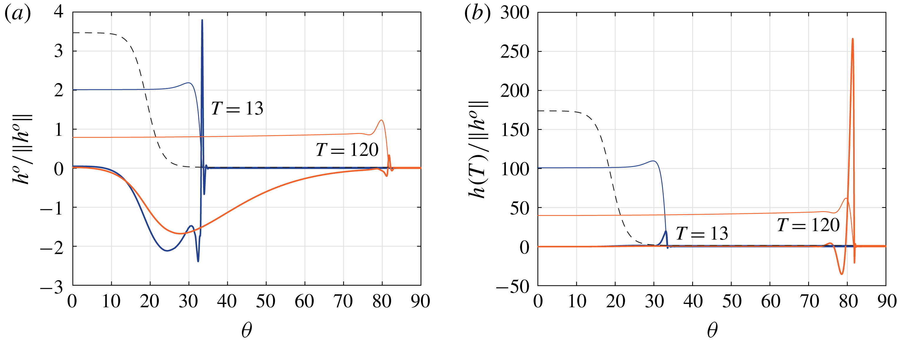
(a) Optimal substrate
 $h^{o}$
and (b) optimal responses
 $h(T)$
for the time horizons
 $T=13$
and
 $120$
(thick solid lines), normalized by the initial
 $L_{2}$
-norm of the substrate perturbation
 $\Vert h^{o}\Vert$
. The thin solid lines indicate the base flow profile
 $H$
at times
 $T$
and the black dashed lines are the base flow at
 $t=0$
(in arbitrary units). Here
 $\unicode[STIX]{x1D6FD}=2$
.

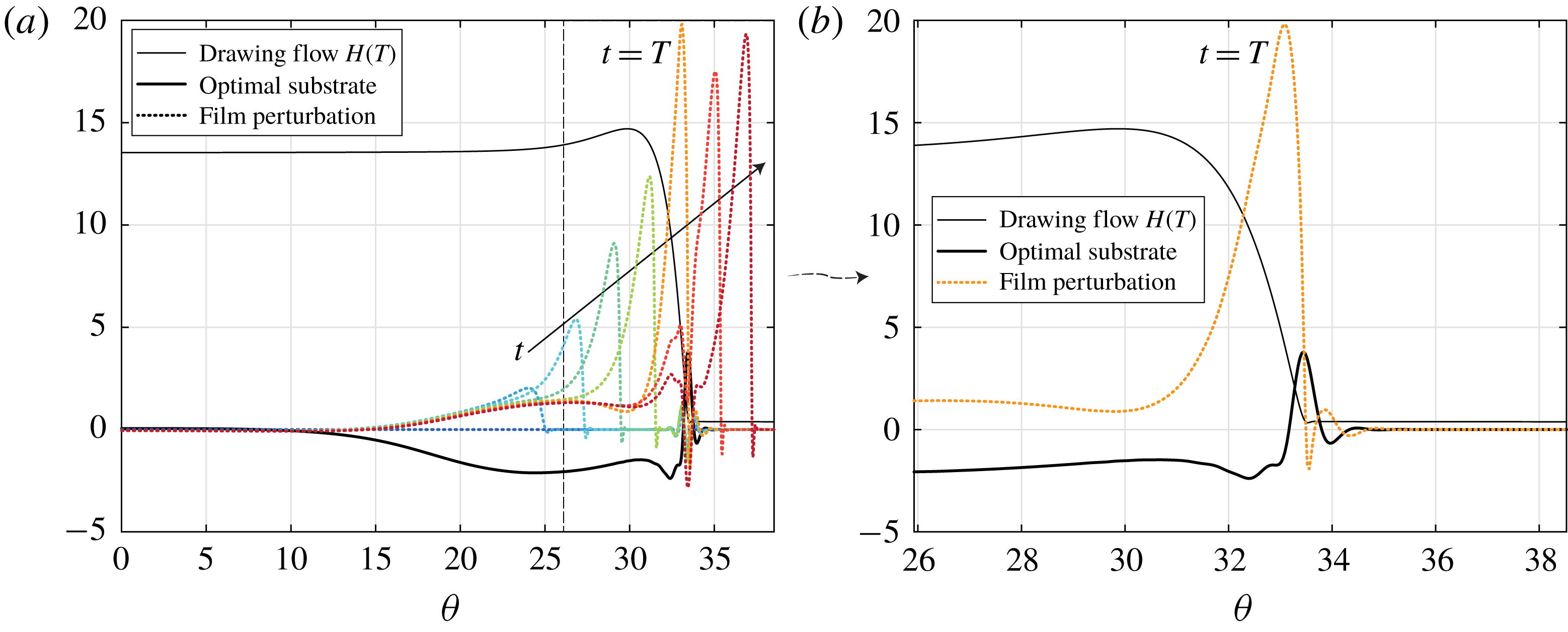
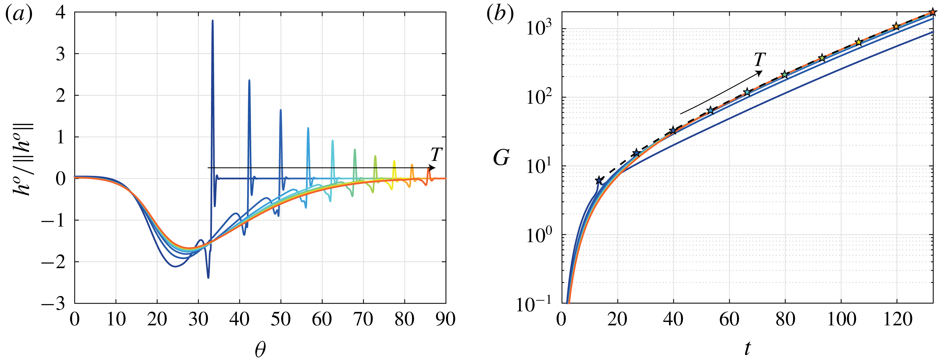
Like the optimal initial conditions of § 4.4.1, the optimal substrate topographies are composed of two parts: a wide-bump perturbation and a localized perturbation at the location reached by the draining flow at the time
 $t=T$
(see figure 15
a). The latter is particularly evident in the optimal substrate profiles for short time horizons, whereas the former mainly composes the optimal substrates for late time horizons. In contrast to the optimal initial conditions (see for instance figure 7), the wide-bump perturbation has an opposite sign with respect to the film-thickness response (see figure 15
b).
(a) Evolution of the film perturbations
 $h$
(dotted lines) over the optimal substrate
 $h^{o}(T)$
for
 $T=13$
(thick solid line), both normalized by the initial
 $L_{2}$
-norm of the substrate perturbation
 $\Vert h^{o}\Vert$
, for the times
 $t=0$
,
 $2.6$
,
 $5.3$
,
 $8.0$
,
 $10.6$
,
 $13$
,
 $15.9$
and
 $18.6$
. (b) Zoom on the optimal response
 $h(T)$
. The thin solid line indicates the base flow profile
 $H(T)$
(in arbitrary units). Here
 $\unicode[STIX]{x1D6FD}=2$
.

Film-thickness perturbations grow, from an initially zero profile, following a two-step process (see figure 16 a). First, when the fluid flows over the wide bump of the substrate, a perturbation ridge forms under the effect of the capillary pressure gradient due to the wide-bump curvature. Kalliadasis, Bielarz & Homsy (Reference Kalliadasis, Bielarz and Homsy2000) also observed the formation of a large asymmetric capillary ridge right before a step down in the substrate. The formed perturbation ridge grows with time, replenished by the base flow. Second, when the perturbation ridge reaches the localized substrate perturbation, it experiences a very fast growth (see orange dotted curve in figure 16). The second step can be understood with the help of figure 16(b). The optimal substrate presents a trough in the base-flow inner region, followed by a steep front at the virtual contact line. Therefore, the fluid perturbation reaching this location suddenly increases in amplitude while meeting the localized substrate obstacle. Note that the peak in the film perturbation is always located upstream with respect to the peak in the optimal substrate. Once the perturbation has passed the localized substrate peak, the perturbation decays, before increasing again due to the instability of the three-dimensional advancing perturbed ridge. In the outer region, where the base flow reaches a uniform (but thinning) profile, the perturbation relaxes to the reversed shape as that of the substrate, in particular over the highly oscillating region of the substrate, due to surface-tension effects. The relative contribution to the perturbation growth induced by the first or second step depends on the intensity of the wide-bump and localized perturbations, and is therefore dependent on wavenumber.
In a way similar to that for the gain evolutions of the optimal initial conditions of figure 9, the larger the time horizon, the larger and more similar the gain evolutions induced by the optimal substrate perturbations due to their weak dependence on
 $T$
(see figure 17).
Optimal substrate
 $h^{o}(T)$
, normalized by the initial
 $L_{2}$
-norm of the substrate perturbation
 $\Vert h^{o}\Vert$
(a) and gain
 $G$
(b) for the time horizons
 $T=13$
,
 $27$
,
 $40$
,
 $53$
,
 $66$
,
 $80$
,
 $93$
,
 $106$
,
 $120$
and
 $133$
. The stars indicate the optimal gains
 $G_{max}=G(T)$
. The black dashed line corresponds to the envelope of the gains
 $G_{max}$
. Here
 $\unicode[STIX]{x1D6FD}=2$
.

5.5.2 Optimal spanwise wavenumber
Optimal substrate
 $h^{o}(T)$
, normalized by the initial
 $L_{2}$
-norm of the substrate perturbation
 $\Vert h^{o}\Vert$
for the time horizons
 $T=13$
,
 $27$
,
 $40$
,
 $53$
,
 $66$
,
 $80$
,
 $93$
,
 $106$
,
 $120$
and
 $133$
for
 $\unicode[STIX]{x1D6FD}=$
(a) 0.5, (b) 2, (c) 4 and (d) 6. The stars indicate the thickest location of the wide-bump perturbation.

The effect of the spanwise wavenumber on the optimal substrate topographies is very similar to that discussed in § 4.4.2 for the optimal initial conditions. In particular, the maximum of the wide-bump perturbation is located at a polar location which increases with
 $\unicode[STIX]{x1D6FD}$
(see stars in figure 18). For too small or too large spanwise wavenumbers, the wide-bump perturbations are not optimal and the largest disturbance growth is given by a sharp localized substrate perturbation at the location reached by the draining flow at
 $t=T$
. Furthermore, the disturbance gain
 $G$
obtained by the wide-bump perturbations is significantly larger and less horizon-dependent than that induced by the localized perturbations (see figure 19).
Gain
 $G$
for the time horizons
 $T=13$
,
 $27$
,
 $40$
,
 $53$
,
 $66$
,
 $80$
,
 $93$
,
 $106$
,
 $120$
and
 $133$
for
 $\unicode[STIX]{x1D6FD}=$
(a) 0.5, (b) 2, (c) 4 and (d) 6. The stars indicate the optimal gains
 $G_{max}=G(T)$
. The black dashed lines correspond to the envelope of the gains
 $G_{max}$
.

Envelopes
 $G_{max}(\unicode[STIX]{x1D6FD},t)$
for the gain evolutions induced by substrate-topography perturbations for
 $\unicode[STIX]{x1D6FD}=0.5$
,
 $2$
,
 $2.5$
,
 $3$
,
 $3.5$
,
 $4$
,
 $4.5$
,
 $5$
,
 $5.5$
,
 $6$
,
 $6.5$
,
 $7$
,
 $8$
,
 $9$
and
 $10$
. The largest optimal gains obtained by the transient growth analysis, and the corresponding optimal wavenumbers
 $\unicode[STIX]{x1D6FD}$
, at every considered time, are indicated by the black symbols. The optimal wavenumbers given by inclined-plane theory with
 $\unicode[STIX]{x1D6FD}=0.5/\ell _{c}$
(red dashed line) and
 $\unicode[STIX]{x1D6FD}=0.5/\ell$
(red solid line) are also represented.

The envelopes of the optimal gains
 $G_{max}$
as a function of time
 $t$
and spanwise wavenumber
 $\unicode[STIX]{x1D6FD}$
are shown in figure 20. It can be noted that the optimal
 $\unicode[STIX]{x1D6FD}$
presents an evolution similar to that for the optimal initial conditions shown in figure 12. The optimal spanwise wavenumber initially decreases at short times before increasing for
 $t\gtrsim 40$
. As discussed in § 4.4.2, this evolution can be rationalized by considering the dependence of the most amplified spanwise wavenumber on the length of the capillary ridge.
Nonetheless, the precise value of the optimal spanwise wavenumber
 $\unicode[STIX]{x1D6FD}$
of substrate-topography perturbations at a given time
 $t$
is slightly smaller than that obtained for the optimal initial conditions. Hence, the expected fingering wavelength induced by substrate-topography perturbations is slightly larger than that induced by the initial film-thickness perturbations. For instance, the predicted wavelength induced by substrate-topography perturbations in the temporal range
 $t=47{-}100$
, which corresponds to the finger formation time in the experiment of Takagi & Huppert (Reference Takagi and Huppert2010), lies in the range 4.1–5.7 cm (
 $\unicode[STIX]{x1D6FD}=2.5{-}3.5$
) (see figure 20). This wavelength is closer to the experimentally observed one of about 5 cm. Therefore, we can conjecture that the fingering wavelength observed in the experiments of Takagi & Huppert (Reference Takagi and Huppert2010) is probably due to random substrate perturbations that project themselves on this most amplified mode, rather than to initial film-thickness perturbations alone.
Finally, it has to be mentioned that reducing the Bond number induces larger fingering wavelengths and smaller gains. The stronger the capillary effects, the larger the characteristic size of the perturbation’s structures and the smoother the capillary-ridge profile. On the other hand, reducing the film aspect ratio induces smaller fingering wavelengths and larger gains. The perturbations are more localized and can grow over longer times. These effects also hold for the optimal initial conditions analysis of § 4. More details of the effects of
 $Bo$
and
 $\unicode[STIX]{x1D6FF}$
are given in appendix E.
6 Conclusions
The fingering instability of a Newtonian thin viscous film flowing on a horizontal cylindrical substrate has been investigated. In contrast to the classic fingering instability on an inclined plane, where the advancing capillary ridge can be considered as quasi-static and its stability is well captured by a modal linear stability analysis, the flow on a cylinder is intrinsically unsteady and a non-modal transient growth analysis has to be undertaken. The novelty of our work lies in the generalization of the fingering instability to curved substrates, including the optimization of substrate-topography perturbations, which have been scarcely investigated in the literature despite their practical interest.
First, we have characterized the axially invariant draining flow. We assume total wetting, i.e. the absence of a contact line, by imposing a precursor film downstream of the advancing ridge (Troian et al.
Reference Troian, Herbolzheimer, Safran and Joanny1989; Bertozzi & Brenner Reference Bertozzi and Brenner1997; Spaid & Homsy Reference Spaid and Homsy1996). As for the flow over an inclined plane, the draining solution is composed of an outer solution, where the film is smooth, and an inner solution close to the capillary ridge, where the film thickness experiences large variations to match the precursor film thickness (Troian et al.
Reference Troian, Herbolzheimer, Safran and Joanny1989). Since the dynamics in the outer region is governed only by the balance of gravity and viscous stresses, we have been able to derive an approximate solution for the film thickness in this region. Excellent agreement is found for the temporal and spatial variations of the film thickness, as well as for the front position. Both the film thickness and the front velocity decrease in time as
 $t^{-1/2}$
. We have shown that the cylindrical geometry of the substrate induces a non-monotonic temporal variation of the characteristic length of the capillary ridge, where the capillary pressure term and the variation of the hydrostatic pressure have to be considered as well. At short times, when the capillary ridge is on a rather horizontal substrate, the length of the inner region is given by the capillary length, obtained by balancing the capillary pressure with the variation of the hydrostatic pressure. However, at long times, when the capillary ridge is on a rather inclined substrate, its characteristic length is given by balancing the capillary pressure with the drainage, and it decreases in time as
 $t^{-1/3}$
.
Second, the instability of the advancing ridge has been first investigated by performing an optimal transient growth analysis for the perturbations of the initial film thickness. We have found that an optimal spanwise wavenumber
 $\unicode[STIX]{x1D6FD}$
exists at every time: it decreases at short times and increases at large ones. The crossover between the two behaviours is in good agreement with the crossover between the two characteristic lengths of the capillary ridge, assuming that the modal linear stability analysis of the flow over an inclined plane would predict an optimal spanwise wavenumber
 $\unicode[STIX]{x1D6FD}=0.5/\ell$
(Troian et al.
Reference Troian, Herbolzheimer, Safran and Joanny1989; Spaid & Homsy Reference Spaid and Homsy1996). However, the optimal
 $\unicode[STIX]{x1D6FD}$
found by the optimal transient growth analysis at short times is much larger. The draining flow experiences very large variations and the capillary ridge is far from a travelling-wave solution; the classic modal stability analysis fails. At large times, the optimal spanwise wavenumber predicted by our analysis is closer to that of the modal analysis since the variations in the draining flow are slower. Yet, the optimal spanwise wavenumber is always smaller than that predicted by the modal analysis due to the time-dependent history of the flow. The most amplified mode from a modal analysis at one time instant will be inefficient for later times as the linear operator has changed.
Strikingly, we have been able to show that the optimal spanwise wavenumber corresponds to the optimal initial perturbations of the film thickness which is the least dependent on time horizon. These universal optimal initial conditions correspond to wide-bump perturbations of the precursor film thickness and are therefore efficient over the entire time the capillary ridge takes to travel along them. Furthermore, we have observed that the location where the wide-bump perturbations are the largest increases with
 $\unicode[STIX]{x1D6FD}$
. This is very likely to be related to the result of the modal linear stability analysis for the flow over an inclined plane, where large spanwise wavenumbers are found to be more effective at large inclination angles. The finding of optimal perturbations located in the precursor film region is in agreement with the sensitivity of the instability growth on the detail of the perturbations at the moving virtual contact line (Bertozzi & Brenner Reference Bertozzi and Brenner1997).
Finally, we have answered the question of the optimal substrate-topography perturbations. The latter are in fact more relevant in practice as imposing an initial disturbance of the film thickness is not an easy task. In this work, we considered only substrate perturbations whose characteristic length can be well resolved numerically or manufactured. Smaller-scale perturbations are in fact intrinsic to the material and only result in a slightly larger growth. By performing an optimal transient growth analysis with an additional forcing term due to the substrate perturbations, we have shown that the optimal substrate-topography perturbations are composed of structures similar to those of the optimal initial film-thickness disturbances, yet of opposite sign. The optimal spanwise wavenumber follows a similar temporal dependence as for the optimal initial film-thickness perturbations. However, the precise value of
 $\unicode[STIX]{x1D6FD}$
for a given time is smaller. Hence, if the substrate topography is perturbed rather than the initial film thickness profile, the resulting fingering wavelength is slightly larger. The predicted wavelength induced by the substrate-topography perturbations is in good agreement with the experimental finding of Takagi & Huppert (Reference Takagi and Huppert2010).
To conclude, the appearing fingering wavelength depends on the disturbance amplitude. For low disturbance amplitude, a large growth will be necessary and thus a large wavelength will appear, while for a large disturbance amplitude, a small growth suffices for finger formation at short times with a small wavelength. The most amplified wavelength increases with decreasing Bond numbers and increasing film aspect ratios, wheres the optimal gain decreases with decreasing
 $Bo$
and increasing
 $\unicode[STIX]{x1D6FF}$
. Furthermore, it has to be observed that the gain obtained by the substrate perturbations is smaller than that obtained by directly perturbing the film thickness, which remains the most effective way to promote finger formation.
Our current efforts are directed towards considering the robust control of this problem (Bewley, Temam & Ziane Reference Bewley, Temam and Ziane2000), i.e. finding the optimal substrate to stabilize the most dangerous perturbation in order to suppress the fingering formation, a problem of critical practical importance. Furthermore, it would be very interesting to generalize the present work for the case of a spherical substrate treated by Takagi & Huppert (Reference Takagi and Huppert2010), where the perimeter of the advancing ridge increases in time and the fingering wavenumber can take only discrete values. The problem in spherical coordinates shares some analogies with the splashing of a droplet on a rigid substrate, where a radially expanding lamella, similar to an advancing ridge, also forms. The lamella might eventually dewet the substrate and eject smaller droplets following a capillary instability of the rim (Riboux & Gordillo Reference Riboux and Gordillo2014, Reference Riboux and Gordillo2015). However, inertial effects have to be considered for the splashing of a drop.
Acknowledgements
We would like to acknowledge P.-T. Brun for motivating us in this project and the anonymous referees for the valuable comments that helped to improve the manuscript. This work was funded by ERC grant no. SIMCOMICS 280117 and by Swiss National Science Foundation grant no. 200021_178971.
Appendix A. Linear operators
The linear operator for the film perturbation
 $h$
in (4.3) and (5.5) is given by
 $$\begin{eqnarray}\displaystyle L & = & \displaystyle -\frac{2\unicode[STIX]{x1D6FD}^{2}\unicode[STIX]{x1D6FF}^{2}H^{3}}{3Bo}\frac{\unicode[STIX]{x2202}^{2}}{\unicode[STIX]{x2202}\unicode[STIX]{x1D703}^{2}}-\frac{\unicode[STIX]{x1D6FD}^{2}\unicode[STIX]{x1D6FF}^{2}H^{2}H_{\unicode[STIX]{x1D703}}}{Bo}\frac{\unicode[STIX]{x2202}}{\unicode[STIX]{x2202}\unicode[STIX]{x1D703}}-\frac{\unicode[STIX]{x1D6FD}^{2}\unicode[STIX]{x1D6FF}^{2}H^{3}}{3Bo}+\frac{\unicode[STIX]{x1D6FF}^{4}H^{3}}{3Bo}\frac{\unicode[STIX]{x2202}^{4}}{\unicode[STIX]{x2202}\unicode[STIX]{x1D703}^{4}}+\frac{\unicode[STIX]{x1D6FF}^{4}H^{2}H_{\unicode[STIX]{x1D703}\unicode[STIX]{x1D703}\unicode[STIX]{x1D703}\unicode[STIX]{x1D703}}}{Bo}\nonumber\\ \displaystyle & & \displaystyle +\,\frac{\unicode[STIX]{x1D6FF}^{4}H^{2}H_{\unicode[STIX]{x1D703}\unicode[STIX]{x1D703}\unicode[STIX]{x1D703}}}{Bo}\frac{\unicode[STIX]{x2202}}{\unicode[STIX]{x2202}\unicode[STIX]{x1D703}}+\frac{\unicode[STIX]{x1D6FF}^{4}H^{2}H_{\unicode[STIX]{x1D703}}}{Bo}\frac{\unicode[STIX]{x2202}^{3}}{\unicode[STIX]{x2202}\unicode[STIX]{x1D703}^{3}}+\frac{2\unicode[STIX]{x1D6FF}^{4}HH_{\unicode[STIX]{x1D703}}H_{\unicode[STIX]{x1D703}\unicode[STIX]{x1D703}\unicode[STIX]{x1D703}}}{Bo}+\frac{\unicode[STIX]{x1D6FF}^{4}H^{3}}{3Bo}\frac{\unicode[STIX]{x2202}^{2}}{\unicode[STIX]{x2202}\unicode[STIX]{x1D703}^{2}}+\frac{\unicode[STIX]{x1D6FF}^{4}H^{2}H_{\unicode[STIX]{x1D703}\unicode[STIX]{x1D703}}}{Bo}\nonumber\\ \displaystyle & & \displaystyle +\,\frac{2\unicode[STIX]{x1D6FF}^{4}H^{2}H_{\unicode[STIX]{x1D703}}}{Bo}\frac{\unicode[STIX]{x2202}}{\unicode[STIX]{x2202}\unicode[STIX]{x1D703}}+\frac{2\unicode[STIX]{x1D6FF}^{4}HH_{\unicode[STIX]{x1D703}}^{2}}{Bo}-\frac{1}{3}\unicode[STIX]{x1D6FF}H^{3}\cos \unicode[STIX]{x1D703}\frac{\unicode[STIX]{x2202}^{2}}{\unicode[STIX]{x2202}\unicode[STIX]{x1D703}^{2}}-\unicode[STIX]{x1D6FF}H^{2}\cos \unicode[STIX]{x1D703}H_{\unicode[STIX]{x1D703}\unicode[STIX]{x1D703}}\nonumber\\ \displaystyle & & \displaystyle +\,\frac{1}{3}\unicode[STIX]{x1D6FF}H^{3}\sin \unicode[STIX]{x1D703}\frac{\unicode[STIX]{x2202}}{\unicode[STIX]{x2202}\unicode[STIX]{x1D703}}+\unicode[STIX]{x1D6FF}H^{2}\sin \unicode[STIX]{x1D703}H_{\unicode[STIX]{x1D703}}-2\unicode[STIX]{x1D6FF}H^{2}\cos \unicode[STIX]{x1D703}H_{\unicode[STIX]{x1D703}}\frac{\unicode[STIX]{x2202}}{\unicode[STIX]{x2202}\unicode[STIX]{x1D703}}-2\unicode[STIX]{x1D6FF}H\cos \unicode[STIX]{x1D703}H_{\unicode[STIX]{x1D703}}^{2}\nonumber\\ \displaystyle & & \displaystyle +\,H^{2}\cos \unicode[STIX]{x1D703}+H^{2}\sin \unicode[STIX]{x1D703}\frac{\unicode[STIX]{x2202}}{\unicode[STIX]{x2202}\unicode[STIX]{x1D703}}+2H\sin \unicode[STIX]{x1D703}H_{\unicode[STIX]{x1D703}}-\frac{\unicode[STIX]{x1D6FD}^{4}\unicode[STIX]{x1D6FF}^{2}H^{3}H_{\unicode[STIX]{x1D703}}^{2}}{6Bo}+\frac{\unicode[STIX]{x1D6FD}^{4}H^{3}}{3Bo}\nonumber\\ \displaystyle & & \displaystyle +\,\frac{\unicode[STIX]{x1D6FD}^{2}\unicode[STIX]{x1D6FF}^{4}H^{3}H_{\unicode[STIX]{x1D703}}H_{\unicode[STIX]{x1D703}\unicode[STIX]{x1D703}\unicode[STIX]{x1D703}}}{3Bo}+\frac{2\unicode[STIX]{x1D6FD}^{2}\unicode[STIX]{x1D6FF}^{4}H^{3}H_{\unicode[STIX]{x1D703}}H_{\unicode[STIX]{x1D703}\unicode[STIX]{x1D703}}}{3Bo}\frac{\unicode[STIX]{x2202}}{\unicode[STIX]{x2202}\unicode[STIX]{x1D703}}+\frac{\unicode[STIX]{x1D6FD}^{2}\unicode[STIX]{x1D6FF}^{4}H^{3}H_{\unicode[STIX]{x1D703}}^{2}}{6Bo}\frac{\unicode[STIX]{x2202}^{2}}{\unicode[STIX]{x2202}\unicode[STIX]{x1D703}^{2}}\nonumber\\ \displaystyle & & \displaystyle +\,\frac{\unicode[STIX]{x1D6FD}^{2}\unicode[STIX]{x1D6FF}^{4}H^{3}H_{\unicode[STIX]{x1D703}\unicode[STIX]{x1D703}}^{2}}{3Bo}+\frac{\unicode[STIX]{x1D6FD}^{2}\unicode[STIX]{x1D6FF}^{4}H^{2}H_{\unicode[STIX]{x1D703}}^{2}H_{\unicode[STIX]{x1D703}\unicode[STIX]{x1D703}}}{Bo}+\frac{\unicode[STIX]{x1D6FD}^{2}\unicode[STIX]{x1D6FF}^{4}H^{2}H_{\unicode[STIX]{x1D703}}^{3}}{2Bo}\frac{\unicode[STIX]{x2202}}{\unicode[STIX]{x2202}\unicode[STIX]{x1D703}}+\frac{\unicode[STIX]{x1D6FD}^{2}\cos \unicode[STIX]{x1D703}H^{3}}{3\unicode[STIX]{x1D6FF}}.\end{eqnarray}$$
Subscripts with
 $\unicode[STIX]{x1D703}$
correspond to spatial derivatives of the drainage solution
 $H$
.
The linear operator for the substrate perturbation
 $h^{o}$
in (5.5) is given by
 $$\begin{eqnarray}\displaystyle L^{o} & = & \displaystyle -\frac{2\unicode[STIX]{x1D6FD}^{2}\unicode[STIX]{x1D6FF}^{2}H^{3}}{3Bo}\frac{\unicode[STIX]{x2202}^{2}}{\unicode[STIX]{x2202}\unicode[STIX]{x1D703}^{2}}-\frac{\unicode[STIX]{x1D6FD}^{2}\unicode[STIX]{x1D6FF}^{2}H_{\unicode[STIX]{x1D703}}H^{2}}{Bo}\frac{\unicode[STIX]{x2202}}{\unicode[STIX]{x2202}\unicode[STIX]{x1D703}}-\frac{\unicode[STIX]{x1D6FD}^{2}\unicode[STIX]{x1D6FF}^{2}H^{3}}{3Bo}+\frac{\unicode[STIX]{x1D6FF}^{4}H^{3}}{3Bo}\frac{\unicode[STIX]{x2202}^{4}}{\unicode[STIX]{x2202}\unicode[STIX]{x1D703}^{4}}+\frac{\unicode[STIX]{x1D6FF}^{4}H_{\unicode[STIX]{x1D703}}H^{2}}{Bo}\frac{\unicode[STIX]{x2202}^{3}}{\unicode[STIX]{x2202}\unicode[STIX]{x1D703}^{3}}\nonumber\\ \displaystyle & & \displaystyle +\,\frac{\unicode[STIX]{x1D6FF}^{4}H^{3}}{3Bo}\frac{\unicode[STIX]{x2202}^{2}}{\unicode[STIX]{x2202}\unicode[STIX]{x1D703}^{2}}+\frac{\unicode[STIX]{x1D6FF}^{4}H_{\unicode[STIX]{x1D703}}H^{2}}{Bo}\frac{\unicode[STIX]{x2202}}{\unicode[STIX]{x2202}\unicode[STIX]{x1D703}}+\frac{1}{3}\unicode[STIX]{x1D6FF}^{2}\sin \unicode[STIX]{x1D703}H^{4}\frac{\unicode[STIX]{x2202}}{\unicode[STIX]{x2202}\unicode[STIX]{x1D703}}-\frac{1}{3}\unicode[STIX]{x1D6FF}\cos \unicode[STIX]{x1D703}H^{3}\frac{\unicode[STIX]{x2202}^{2}}{\unicode[STIX]{x2202}\unicode[STIX]{x1D703}^{2}}\nonumber\\ \displaystyle & & \displaystyle -\,\unicode[STIX]{x1D6FF}\cos \unicode[STIX]{x1D703}H_{\unicode[STIX]{x1D703}}H^{2}\frac{\unicode[STIX]{x2202}}{\unicode[STIX]{x2202}\unicode[STIX]{x1D703}}+\frac{1}{3}\unicode[STIX]{x1D6FD}^{2}\sin \unicode[STIX]{x1D703}H^{4}\frac{\unicode[STIX]{x2202}}{\unicode[STIX]{x2202}\unicode[STIX]{x1D703}}-\frac{\unicode[STIX]{x1D6FD}^{4}\unicode[STIX]{x1D6FF}^{2}H_{\unicode[STIX]{x1D703}}^{2}H^{3}}{6Bo}+\frac{\unicode[STIX]{x1D6FD}^{4}H^{3}}{3Bo}+\frac{2}{3}\unicode[STIX]{x1D6FF}\sin \unicode[STIX]{x1D703}H^{3}\frac{\unicode[STIX]{x2202}}{\unicode[STIX]{x2202}\unicode[STIX]{x1D703}}\nonumber\\ \displaystyle & & \displaystyle +\,\frac{\unicode[STIX]{x1D6FD}^{2}\unicode[STIX]{x1D6FF}^{4}H_{\unicode[STIX]{x1D703}}H_{\unicode[STIX]{x1D703}\unicode[STIX]{x1D703}\unicode[STIX]{x1D703}}H^{3}}{3Bo}+\frac{2\unicode[STIX]{x1D6FD}^{2}\unicode[STIX]{x1D6FF}^{4}H_{\unicode[STIX]{x1D703}}H_{\unicode[STIX]{x1D703}\unicode[STIX]{x1D703}}H^{3}}{3Bo}\frac{\unicode[STIX]{x2202}}{\unicode[STIX]{x2202}\unicode[STIX]{x1D703}}+\frac{\unicode[STIX]{x1D6FD}^{2}\unicode[STIX]{x1D6FF}^{4}H_{\unicode[STIX]{x1D703}}^{2}H^{3}}{6Bo}\frac{\unicode[STIX]{x2202}^{2}}{\unicode[STIX]{x2202}\unicode[STIX]{x1D703}^{2}}\nonumber\\ \displaystyle & & \displaystyle +\,\frac{\unicode[STIX]{x1D6FD}^{2}\unicode[STIX]{x1D6FF}^{4}H_{\unicode[STIX]{x1D703}\unicode[STIX]{x1D703}}^{2}H^{3}}{3Bo}+\frac{\unicode[STIX]{x1D6FD}^{2}\unicode[STIX]{x1D6FF}^{4}H_{\unicode[STIX]{x1D703}}^{2}H_{\unicode[STIX]{x1D703}\unicode[STIX]{x1D703}}H^{2}}{Bo}+\frac{\unicode[STIX]{x1D6FD}^{2}\unicode[STIX]{x1D6FF}^{4}H_{\unicode[STIX]{x1D703}}^{3}H^{2}}{2Bo}\frac{\unicode[STIX]{x2202}}{\unicode[STIX]{x2202}\unicode[STIX]{x1D703}}+\frac{\unicode[STIX]{x1D6FD}^{2}\cos \unicode[STIX]{x1D703}H^{3}}{3\unicode[STIX]{x1D6FF}}.\end{eqnarray}$$
Appendix B. Derivation of the lubrication equation for a perturbed substrate topography
The free surface is defined by
 $F=r^{\ast }-(R+\bar{H}^{\ast }+\bar{H}^{o\ast })=0$
. We assume that the substrate perturbations
 $\bar{H^{o\ast }}$
are infinitesimally small such that the base flow
 $H^{\ast }$
discussed in § 3 is unaffected. Furthermore, since a linear problem is eventually derived for the optimal substrate perturbations analysis, only linear terms in the substrate-topography perturbations are considered.
At leading order, the normal to the fluid’s interface reads
 $$\begin{eqnarray}\displaystyle \boldsymbol{n}^{\ast }=\frac{1}{\sqrt{1+\left(\displaystyle \frac{\bar{H}_{\unicode[STIX]{x1D703}}^{\ast }}{R}\right)^{2}+\bar{H}_{z^{\ast }}^{\ast 2}}}\left(1,-\frac{\bar{H}_{\unicode[STIX]{x1D703}}^{\ast }+\bar{H}_{\unicode[STIX]{x1D703}}^{o\ast }}{R},-\bar{H}_{z^{\ast }}^{\ast }-\bar{H}_{z^{\ast }}^{o\ast }\right)^{\text{T}} & & \displaystyle\end{eqnarray}$$
and the curvature is given by
 $\bar{\unicode[STIX]{x1D705}}^{\ast }=-\unicode[STIX]{x1D735}^{\ast }\boldsymbol{\cdot }\boldsymbol{n}^{\ast }$
.
The polar component of the drainage term
 $\text{III}$
of (2.1) now reads
 $$\begin{eqnarray}\displaystyle \unicode[STIX]{x1D70C}g\sin \unicode[STIX]{x1D703}-\frac{\unicode[STIX]{x1D70C}g\cos \unicode[STIX]{x1D703}\bar{H}_{\unicode[STIX]{x1D703}}^{o\ast }}{R}, & & \displaystyle\end{eqnarray}$$
whereas the drainage in the axial direction is no longer zero, but is
 $$\begin{eqnarray}\displaystyle -\unicode[STIX]{x1D70C}g\cos \unicode[STIX]{x1D703}\bar{H}_{z^{\ast }}^{o\ast }. & & \displaystyle\end{eqnarray}$$
The variation of the hydrostatic pressure in the polar direction becomes
 $$\begin{eqnarray}\displaystyle -\frac{\unicode[STIX]{x1D70C}g\cos \unicode[STIX]{x1D703}\bar{H}_{\unicode[STIX]{x1D703}}^{\ast }}{R}+\frac{\unicode[STIX]{x1D70C}g\sin \unicode[STIX]{x1D703}\bar{H}^{\ast }}{R}-\frac{\unicode[STIX]{x1D70C}g\cos \unicode[STIX]{x1D703}\bar{H}^{\ast }\bar{H}_{\unicode[STIX]{x1D703}}^{o\ast }}{R^{2}}-\frac{\unicode[STIX]{x1D70C}g\sin \unicode[STIX]{x1D703}\bar{H}_{\unicode[STIX]{x1D703}}^{\ast }\bar{H}_{\unicode[STIX]{x1D703}}^{o\ast }}{R^{2}}-\frac{\unicode[STIX]{x1D70C}g\sin \unicode[STIX]{x1D703}\bar{H}^{\ast }\bar{H}_{\unicode[STIX]{x1D703}\unicode[STIX]{x1D703}}^{o\ast }}{R^{2}}, & & \displaystyle \nonumber\\ \displaystyle & & \displaystyle\end{eqnarray}$$
while that in the axial direction reads
 $$\begin{eqnarray}\displaystyle -\unicode[STIX]{x1D70C}g\cos \unicode[STIX]{x1D703}\bar{H}_{z^{\ast }}^{\ast }-\frac{\unicode[STIX]{x1D70C}g\sin \unicode[STIX]{x1D703}\bar{H}_{z^{\ast }}^{\ast }\bar{H}_{\unicode[STIX]{x1D703}}^{o\ast }}{R}-\frac{\unicode[STIX]{x1D70C}g\sin \unicode[STIX]{x1D703}\bar{H}^{\ast }\bar{H}_{\unicode[STIX]{x1D703}z^{\ast }}^{o\ast }}{R}. & & \displaystyle\end{eqnarray}$$
Putting the hydrodynamic pressure variation and the drainage terms together yields
 $$\begin{eqnarray}\displaystyle & & \displaystyle -\frac{\unicode[STIX]{x1D70C}g\cos \unicode[STIX]{x1D703}\bar{H}_{\unicode[STIX]{x1D703}}^{\ast }}{R}+\frac{\unicode[STIX]{x1D70C}g\sin \unicode[STIX]{x1D703}\bar{H}^{\ast }}{R}-\frac{\unicode[STIX]{x1D70C}g\cos \unicode[STIX]{x1D703}\bar{H}^{\ast }\bar{H}_{\unicode[STIX]{x1D703}}^{o\ast }}{R^{2}}-\frac{\unicode[STIX]{x1D70C}g\sin \unicode[STIX]{x1D703}\bar{H}_{\unicode[STIX]{x1D703}}^{\ast }\bar{H}_{\unicode[STIX]{x1D703}}^{o\ast }}{R^{2}}-\frac{\unicode[STIX]{x1D70C}g\sin \unicode[STIX]{x1D703}\bar{H}^{\ast }\bar{H}_{\unicode[STIX]{x1D703}\unicode[STIX]{x1D703}}^{o\ast }}{R^{2}}\nonumber\\ \displaystyle & & \displaystyle \quad +\,\unicode[STIX]{x1D70C}g\sin \unicode[STIX]{x1D703}-\frac{\unicode[STIX]{x1D70C}g\cos \unicode[STIX]{x1D703}\bar{H}_{\unicode[STIX]{x1D703}}^{o\ast }}{R}\end{eqnarray}$$
for the polar flux and
 $$\begin{eqnarray}\displaystyle -\unicode[STIX]{x1D70C}g\cos \unicode[STIX]{x1D703}\bar{H}_{z^{\ast }}^{\ast }-\frac{\unicode[STIX]{x1D70C}g\sin \unicode[STIX]{x1D703}\bar{H}_{z^{\ast }}^{\ast }\bar{H}_{\unicode[STIX]{x1D703}}^{o\ast }}{R}-\frac{\unicode[STIX]{x1D70C}g\sin \unicode[STIX]{x1D703}\bar{H}^{\ast }\bar{H}_{\unicode[STIX]{x1D703}z^{\ast }}^{o\ast }}{R}-\unicode[STIX]{x1D70C}g\cos \unicode[STIX]{x1D703}\bar{H}_{z^{\ast }}^{o\ast } & & \displaystyle\end{eqnarray}$$
for the axial flux. Using
 $L=\sqrt{A}$
as characteristic length for the radial and axial directions, one obtains
 $$\begin{eqnarray}\displaystyle \unicode[STIX]{x1D70C}g[\sin \unicode[STIX]{x1D703}(1+\unicode[STIX]{x1D6FF}H)-\unicode[STIX]{x1D6FF}(\cos \unicode[STIX]{x1D703}\bar{H}_{\unicode[STIX]{x1D703}}+\cos \unicode[STIX]{x1D703}\bar{H}_{\unicode[STIX]{x1D703}}^{o})-\unicode[STIX]{x1D6FF}^{2}(\cos \unicode[STIX]{x1D703}\bar{H}\bar{H}_{\unicode[STIX]{x1D703}}^{o}-\sin \unicode[STIX]{x1D703}\bar{H}_{\unicode[STIX]{x1D703}}\bar{H}_{\unicode[STIX]{x1D703}}^{o}-\sin \unicode[STIX]{x1D703}\bar{H}\bar{H}_{\unicode[STIX]{x1D703}\unicode[STIX]{x1D703}}^{o})] & & \displaystyle \nonumber\\ \displaystyle & & \displaystyle\end{eqnarray}$$
for the flux in the polar direction and
 $$\begin{eqnarray}\displaystyle \unicode[STIX]{x1D70C}g[-\cos \unicode[STIX]{x1D703}\bar{H}_{z}-\cos \unicode[STIX]{x1D703}\bar{H}_{z}^{o}-\unicode[STIX]{x1D6FF}(\sin \unicode[STIX]{x1D703}\bar{H}_{z}\bar{H}_{\unicode[STIX]{x1D703}}^{o}+\sin \unicode[STIX]{x1D703}\bar{H}\bar{H}_{\unicode[STIX]{x1D703}z}^{o})] & & \displaystyle\end{eqnarray}$$
for the flux in the axial direction.
In order to simplify the fluxes, we consider the principle of least degeneracy (Van Dyke Reference Van Dyke1975) and keep only the leading-order terms. Note that
 $\sin \unicode[STIX]{x1D703}\bar{H}_{z}\bar{H}_{\unicode[STIX]{x1D703}}^{o}=0$
since the base flow is invariant in the axial direction.
Using the drainage time
 $\unicode[STIX]{x1D70F}_{d}=\unicode[STIX]{x1D707}R/(\unicode[STIX]{x1D70C}gA)$
as characteristic time, as done by Takagi & Huppert (Reference Takagi and Huppert2010), the lubrication equation can be written in the following dimensionless form:
 $$\begin{eqnarray}\displaystyle & & \displaystyle \bar{H}_{t}+\frac{1}{3}\left\{\bar{H}^{3}\left[\frac{\unicode[STIX]{x1D6FF}^{2}}{Bo}\bar{\unicode[STIX]{x1D705}}_{\unicode[STIX]{x1D703}}-\unicode[STIX]{x1D6FF}\cos \unicode[STIX]{x1D703}(\bar{H}_{\unicode[STIX]{x1D703}}+\bar{H}_{\unicode[STIX]{x1D703}}^{o})+\sin \unicode[STIX]{x1D703}\right]\right\}_{\unicode[STIX]{x1D703}}\nonumber\\ \displaystyle & & \displaystyle \quad +\,\frac{1}{3\unicode[STIX]{x1D6FF}}\left\{\bar{H}^{3}\left[\frac{\unicode[STIX]{x1D6FF}}{Bo}\bar{\unicode[STIX]{x1D705}}_{z}-\cos \unicode[STIX]{x1D703}(\bar{H}_{z}+\bar{H}_{z}^{o})-\unicode[STIX]{x1D6FF}\sin \unicode[STIX]{x1D703}\bar{H}\bar{H}_{\unicode[STIX]{x1D703}z}^{o}\right]\right\}_{z}=0.\end{eqnarray}$$
The prefactor
 $1/\unicode[STIX]{x1D6FF}$
in front of the axial flux variation results from the different characteristic length in the polar and axial directions. While the characteristic length in the polar direction is
 $R$
, the axial direction is scaled with the film thickness and therefore with
 $\sqrt{A}$
.
The capillary pressure gradient term is also modified since the curvature depends on
 $\bar{H}^{o}$
as well. The curvature is truncated at the second order in
 $\unicode[STIX]{x1D6FF}$
in order to keep the leading-order dependence of
 $\bar{H}$
and
 $\bar{H}^{o}$
on the polar angle
 $\unicode[STIX]{x1D703}$
:
 $$\begin{eqnarray}\displaystyle \bar{\unicode[STIX]{x1D705}}=-\unicode[STIX]{x1D6FF}+\bar{H}_{zz}+\bar{H}_{zz}^{o}+\unicode[STIX]{x1D6FF}^{2}[\bar{H}+\bar{H}^{o}+\bar{H}_{\unicode[STIX]{x1D703}\unicode[STIX]{x1D703}}+\bar{H}_{\unicode[STIX]{x1D703}\unicode[STIX]{x1D703}}^{o}-\bar{H}_{\unicode[STIX]{x1D703}}^{2}(\bar{H}_{zz}+\bar{H}_{zz}^{o})]+O(\unicode[STIX]{x1D6FF}^{3}). & & \displaystyle\end{eqnarray}$$
Appendix C. Numerical methods
The draining base flow is obtained by resolving the nonlinear lubrication (3.1) with the finite element method of COMSOL Multiphysics. Cubic elements with Lagrangian shape functions have been used on a regular grid of characteristic size
 $8\times 10^{-4}$
. The film thickness and curvature are the two resolved variables. The ability of this method to correctly resolve the film-thickness profile is proven by the excellent comparison with respect to the analytical solutions (see § 3 and Balestra et al.
Reference Balestra, Kofman, Brun, Scheid and Gallaire2017). Half of a cylinder is considered with boundary conditions
 $H_{\unicode[STIX]{x1D703}}=H_{\unicode[STIX]{x1D703}\unicode[STIX]{x1D703}\unicode[STIX]{x1D703}}=0$
at
 $\unicode[STIX]{x1D703}=0$
and
 $\unicode[STIX]{x1D703}=\unicode[STIX]{x03C0}$
, such that the flux vanishes at these locations. To avoid dripping phenomena in the lower part of the cylinder, we stop the simulations once the ridge arrives at
 $\unicode[STIX]{x1D703}=\unicode[STIX]{x03C0}/2$
. Only the upper quarter of the cylinder is considered for the optimal transient growth analysis.
In order to have a correct evolution of the disturbances on the draining flow, it is necessary to have a sufficiently fine temporal representation of the draining flow. This is achieved by interpolating the computed draining flow profiles. Due to the hyperbolic character of the equation, the following approach is employed. During the time interval
 $\unicode[STIX]{x0394}t=t^{i+1}-t^{i}$
, the front has travelled by a distance
 $\unicode[STIX]{x0394}\unicode[STIX]{x1D703}_{N}=\unicode[STIX]{x1D703}_{N}^{i+1}-\unicode[STIX]{x1D703}_{N}^{i}$
. The interpolated film thickness is given by
 $$\begin{eqnarray}\displaystyle H(\unicode[STIX]{x1D703},t+\unicode[STIX]{x0394}t/2)=\frac{H(\unicode[STIX]{x1D703},t)+H(\unicode[STIX]{x1D703}+\unicode[STIX]{x0394}\unicode[STIX]{x1D703}_{N},t+\unicode[STIX]{x0394}t)}{2}. & & \displaystyle\end{eqnarray}$$
Note that for
 $t\lessapprox \unicode[STIX]{x1D70F}_{i}$
, the front position is almost not changing, meaning that the interpolation results in the arithmetic mean of
 $H$
at the successive times.
For the optimal transient growth analysis, the linear operators
 $L$
and
 $L^{o}$
are constructed with the obtained draining flow
 $H$
and the linear disturbance equations are integrated in time using a Crank–Nicolson method to minimize numerical diffusion.
In the optimal transient growth algorithm of the substrate-topography perturbations described in § 5.4 we have employed the low-pass filter fir1.m of Matlab with order
 $60$
and a cut-off length of
 $0.0084~\text{rad}^{-1}$
, together with a Chebyshev window with
 $100~\text{dB}$
of attenuation. We used the highest possible cut-off frequency in order to get the finest resolution of the substrate-topography perturbations and we verified that the presented results are rather insensitive to the precise choice of the cut-off frequency. More precisely, a reduction of the cut-off frequency by
 $20\,\%$
only reduces the gain by a maximum of
 $0.13\,\%$
at short times (
 $T=6$
) and only by
 $0.006\,\%$
at longer times (
 $T=53$
). We have also verified that the optimal spanwise wavenumber is never affected by the choice of the cut-off frequency.
Appendix D. Derivation of the adjoint fields for the optimal substrate algorithm
The optimality condition for the augmented Lagrangian (5.7) with respect to
 $\unicode[STIX]{x1D6FF}h$
is found in a very similar way to the derivation for the algorithm giving the optimal initial condition of § 4.3, which is described in great detail in Balestra et al. (Reference Balestra, Brun and Gallaire2016). The only difference is that the initial condition for the film thickness is no longer the variable to be optimized and therefore the augmented Lagrangian does not need to enforce this condition. Note however that, if one would have enforced also the initial condition, the optimality condition with respect to
 $\unicode[STIX]{x1D6FF}h_{0}$
would have indeed given
 $\unicode[STIX]{x1D6FF}h^{\dagger }=0$
.
More interesting is the optimality condition with respect to the substrate perturbation. For the derivation, we will make use of Fréchet derivatives, which for an operator
 $A(s)$
are defined by (see Cossu Reference Cossu2014)
 $$\begin{eqnarray}\displaystyle \left\langle \frac{\unicode[STIX]{x2202}A}{\unicode[STIX]{x2202}s}\biggm\vert\unicode[STIX]{x1D6FF}s\right\rangle =\lim _{\unicode[STIX]{x1D716}\rightarrow 0}\frac{A(s+\unicode[STIX]{x1D716}\unicode[STIX]{x1D6FF}s)-A(s)}{\unicode[STIX]{x1D716}}. & & \displaystyle\end{eqnarray}$$
The variation of
 ${\mathcal{L}}$
with respect to
 $\unicode[STIX]{x1D6FF}h^{o}$
results in
 $$\begin{eqnarray}\displaystyle \left\langle \frac{\unicode[STIX]{x2202}{\mathcal{L}}}{\unicode[STIX]{x2202}h^{o}}\biggm\vert\unicode[STIX]{x1D6FF}h^{o}\right\rangle & = & \displaystyle \left\langle -2h^{o}\frac{\langle h(T)\mid h(T)\rangle }{\langle h^{o}\mid h^{o}\rangle ^{2}}\biggm\vert\unicode[STIX]{x1D6FF}h^{o}\right\rangle -\int _{0}^{T}\langle h^{\dagger }\mid L^{o}\unicode[STIX]{x1D6FF}h^{o}\rangle \,\text{d}t\end{eqnarray}$$
 $$\begin{eqnarray}\displaystyle & = & \displaystyle \left\langle -2h^{o}\frac{\langle h(T)\mid h(T)\rangle }{\langle h^{o}\mid h^{o}\rangle ^{2}}\biggm\vert\unicode[STIX]{x1D6FF}h^{o}\right\rangle -\int _{0}^{T}\langle L^{o\dagger }h^{\dagger }\mid \unicode[STIX]{x1D6FF}h^{o}\rangle \,\text{d}t\end{eqnarray}$$
 $$\begin{eqnarray}\displaystyle & = & \displaystyle \left\langle -2h^{o}\frac{\langle h(T)\mid h(T)\rangle }{\langle h^{o}\mid h^{o}\rangle ^{2}}\mid \unicode[STIX]{x1D6FF}h^{o}\right\rangle -\left\langle \int _{0}^{T}L^{o\dagger }h^{\dagger }\,\text{d}t\biggm\vert\unicode[STIX]{x1D6FF}h^{o}\right\rangle\end{eqnarray}$$
 $$\begin{eqnarray}\displaystyle & = & \displaystyle \left\langle -2h^{o}\frac{\langle h(T)\mid h(T)\rangle }{\langle h^{o}\mid h^{o}\rangle ^{2}}-\int _{0}^{T}L^{o\dagger }h^{\dagger }\,\text{d}t\mid \unicode[STIX]{x1D6FF}h^{o}\right\rangle ,\end{eqnarray}$$
where the definition of the adjoint operator, namely
 $\langle a\mid L^{o}b\rangle =\langle L^{o\dagger }a\mid b\rangle$
, has been used in (D 3). Since the optimal substrate perturbation
 $h^{o}$
is time independent, we can commute temporal integration and spatial integration (through the scalar product) in (D 4). By imposing a vanishing variation of
 ${\mathcal{L}}$
to any
 $\unicode[STIX]{x1D6FF}h^{o}$
, one eventually obtains
 $$\begin{eqnarray}\displaystyle \left\langle \frac{\unicode[STIX]{x2202}{\mathcal{L}}}{\unicode[STIX]{x2202}h^{o}}\biggm\vert\unicode[STIX]{x1D6FF}h^{o}\right\rangle =0,\quad \forall \unicode[STIX]{x1D6FF}h^{o}\Leftrightarrow \frac{h^{o}}{\langle h^{o}|h^{o}\rangle ^{2}}=\frac{1}{-2\langle h(T)\mid h(T)\rangle }\int _{0}^{T}L^{o\dagger }h^{\dagger }\,\text{d}t. & & \displaystyle\end{eqnarray}$$
Appendix E. Effect of the Bond number and film aspect ratio
The results for a smaller Bond number and a smaller film aspect ratio compared to the ones used throughout the study are shown in figures 21 and 22.
As expected, the stronger the capillary effects, the larger the characteristic size of the perturbations, both in the polar and in the axial directions, resulting in a larger optimal spanwise wavelength (compare figure 22(a) to figure 17). The rationale for this behaviour can be again explained using the relation obtained for the thin-film flow on an inclined plane between the the most amplified spanwise wavelength and length of the capillary ridge:
 $\unicode[STIX]{x1D706}^{\ast }\sim \ell ^{\ast }\sim H_{N}^{\ast }(\unicode[STIX]{x1D707}U_{N}^{\ast }/\unicode[STIX]{x1D6FE})^{-1/3}$
(Spaid & Homsy Reference Spaid and Homsy1996). Note that the stronger the capillary effects, the smaller the growth of the perturbations due to the smoother capillary ridge.
Smaller film aspect ratios
 $\unicode[STIX]{x1D6FF}=\sqrt{A}/R$
correspond to smaller film thicknesses compared to the cylinder radius. Keeping in mind that
 $U_{N}^{\ast }\sim \sin \unicode[STIX]{x1D703}_{N}H_{N}^{\ast 2}$
and that mass conservation imposes
 $H_{N}^{\ast }\sim A/(R\unicode[STIX]{x1D703}_{N})$
, one can conclude that when
 $A$
reduces or
 $R$
increases, the film thickness
 $H_{N}^{\ast }$
at a given polar angle reduces and so does the most amplified wavelength. The characteristic length in the polar direction is also reduced and the growth occurs over a longer time, reaching therefore larger values.
(a,c) Optimal substrate
 $h^{o}(T)$
, normalized by the initial
 $L_{2}$
-norm of the substrate perturbation
 $\Vert h^{o}\Vert$
and (b,d) gain
 $G$
for a smaller Bond number,
 $Bo=8$
(a,b) and a smaller film aspect ratio,
 $\unicode[STIX]{x1D6FF}=0.08$
(c,d) compared to the values used throughout the study, namely
 $Bo=15$
and
 $\unicode[STIX]{x1D6FF}=0.15$
. The stars in (b,d) indicate the optimal gains
 $G_{max}=G(T)$
. Here
 $\unicode[STIX]{x1D6FD}=2$
. Note the different temporal scale between (b) and (d). These figures have to be compared to figure 17.

Envelopes
 $G_{max}(\unicode[STIX]{x1D6FD},t)$
for the gain evolutions induced by substrate-topography perturbations as a function of the wavenumber
 $\unicode[STIX]{x1D6FD}$
and time
 $t$
for
 $Bo=8$
and
 $\unicode[STIX]{x1D6FF}=0.15$
(a) and
 $Bo=15$
and
 $\unicode[STIX]{x1D6FF}=0.08$
(b). The largest optimal gains obtained by the transient growth analysis, and the corresponding optimal wavenumbers
 $\unicode[STIX]{x1D6FD}$
, at every considered time, are indicated by the black symbols. These figures have to be compared to figure 20.