Turning Out to Vote: The Costs of Finding and Getting to the Polling Place

HENRY E. BRADY; JOHN E. MCNULTY

doi:10.1017/S0003055410000596

Turning Out to Vote: The Costs of Finding and Getting to the Polling Place

Published online by Cambridge University Press: 15 March 2011

HENRY E. BRADY and

JOHN E. MCNULTY

Show author details

HENRY E. BRADY*: Affiliation:
University of California, Berkeley
JOHN E. MCNULTY*: Affiliation:
Binghamton University
*: Henry E. Brady is Class of 1941 Monroe Deutsch Professor of Political Science and Public Policy, University of California, Berkeley, 210 Barrows Hall, Berkeley, CA 94720 (hbrady@berkeley.edu).
John E. McNulty is Assistant Professor of Political Science, Binghamton University, State University of New York, Binghamton, NY 13902 (jmcnulty@binghamton.edu).

Article contents

Abstract
PAST RESEARCH AND THEORY
APPROACH TO THE EMPIRICAL ANALYSIS
STATISTICAL MATCHING RESULTS
CONCLUSION
Footnotes
References

Rights & Permissions

Abstract

Could changing the locations of polling places affect the outcome of an election by increasing the costs of voting for some and decreasing them for others? The consolidation of voting precincts in Los Angeles County during California's 2003 gubernatorial recall election provides a natural experiment for studying how changing polling places influences voter turnout. Overall turnout decreased by a substantial 1.85 percentage points: A drop in polling place turnout of 3.03 percentage points was partially offset by an increase in absentee voting of 1.18 percentage points. Both transportation and search costs caused these changes. Although there is no evidence that the Los Angeles Registrar of Voters changed more polling locations for those registered with one party than for those registered with another, the changing of polling places still had a small partisan effect because those registered as Democrats were more sensitive to changes in costs than those registered as Republicans. The effects were small enough to allay worries about significant electoral consequences in this instance (e.g., the partisan effect might be decisive in only about one in two hundred contested House elections), but large enough to make it possible for someone to affect outcomes by more extensive manipulation of polling place locations.

Information

Type: Research Article
Information: American Political Science Review , Volume 105 , Issue 1 , February 2011, pp. 115 - 134
DOI: https://doi.org/10.1017/S0003055410000596 [Opens in a new window]
Copyright: Copyright © American Political Science Association 2011

“Officials in two Houston-area elections recently manipulated polling locations to clear the path for their supporters to vote and to toss numerous roadblocks before their opponents.”

—Joe Stinebaker, Associated Press, Dallas Morning News, February 14, 2007

More than 50 years ago, Anthony Downs (Reference Downs1957) argued persuasively that voting incurs both costs and benefits, and when the costs get sufficiently high, rational voters will abstain by not turning out to vote. Because costs may differ across groups, Downs’ insight suggests that partisan politicians might be able to manipulate election dates, places, modes, and times to encourage voting by their supporters and to hinder voting by their opponents (Dunne, Reed, and Wilbanks Reference Dunne, Reed and Wilbanks1997). One often changed feature of voting is the location of the polling place. Could something as simple, trifling, and apparently benign as changing polling place locations in Houston or elsewhere actually affect the number and kinds of people who vote by changing the equilibrium between the costs and benefits of voting?

In theory, even a tiny cost could lead to wholesale abstention (Niemi Reference Niemi1976; Sanders Reference Sanders1980), so low is the probability that one's single vote will affect the outcome of the election and be decisive in producing benefits for the voter. In practice, of course, people do vote, demonstrating that the act of participation is not only an exercise in self-interest, but also provides altruistic, civic-minded, and expressive benefits that overcome the personal costs in information gathering, time expended, distance traveled, and inconvenience incurred (Aldrich Reference Aldrich1993; Blais Reference Blais2000; Fedderson Reference Fedderson2004; Fedderson and Pesendorfer Reference Fedderson and Pesendorfer1996, Reference Fedderson and Pesendorfer1999; Fedderson and Sandroni Reference Fedderson and Sandroni2006; Goodin and Roberts Reference Goodin and Roberts1975; Green and Shapiro Reference Green and Shapiro1994; Leighley and Nagler Reference Leighley and Nagler1992; Palfrey and Rosenthal Reference Palfrey and Rosenthal1995; Riker and Ordeshook Reference Riker and Ordeshook1973; Rosenstone and Hansen Reference Rosenstone and Hansen1993; Uhlaner Reference Uhlaner1989; Verba, Schlozman, and Brady Reference Verba, Schlozman and Brady1995; Wolfinger and Rosenstone Reference Wolfinger and Rosenstone1980). However, these higher-minded motivations are not universally sufficient to overcome the costs of voting for all people. Although turnout rates are highly variable, they never approach 100% in any election of consequence. So, costs do matter for voter turnout, but how much?

The historic California 2003 gubernatorial recall election provided an opportunity to study how voting costs affect voter turnout. In what amounts to a natural experiment, some counties—in order to cut administrative costs—consolidated voting precinctsFootnote ¹ and changed polling locations in ways that nearly randomly assigned increased voting costs to some voters but not others. Los Angeles County, the largest county in the United States, reduced the number of distinct voting precincts by 64% from 5,231 to 1,885, thus changing the location of the polling place for two thirds of the registered voters. We compare 2003 turnout of the “treatment” group, whose polling places changed from their location in 2002 to the 2003 turnout of the “control” group, whose polling place in 2003 remained the same as in 2002.

Although this change in polling places is not a perfect natural experiment, it is about as close as we can come with observational data. Furthermore, using statistical matching methods, we can create substantial similarity (or “balance”) between the treatment and control groups. Consequently, these data provide us with a strong inference that changing polling places in Los Angeles County reduced turnout by a substantial 1.85% among those who had their polling places changed. Voting at the polling place decreased even more, by 3.03%; however, an increase in absentee voting of 1.18% made up for some of this reduction. In addition, the substitution of absentee voting for polling place voting is greatest among older and middle-age people, whereas younger people are more inclined to simply not vote at all.

The change in polling places had two effects we expected: a transportation effect resulting from the change in distance to the polling place and a search effect resulting from the costs of finding and going to a new polling place. About 60% of the 3.03% reduction in turnout at the polling place is due to the search effect (of about 1.8%), and the impact of the search effect is about two and one-half times larger than the transportation effect for the average person who experienced an increased distance to the polling place of about one sixth of a mile. The two effects are roughly equal for someone who had an increased distance to the polling place of about a mile. The overall reduction in not voting of about 1.85% is almost entirely due to the search effect (about 1.4%) because the decision not to vote appears to be essentially unaffected by the distance to the polling place. People make a decision about voting or not voting based on the increased search costs from having their polling place moved, and if they decide to vote, they choose absentee or polling place voting based on both search and travel costs.

The change also had some partisan effects. There is no indication that the Los Angeles County Registrar of Voters manipulated polling locations so as to change more polling locations for those registered with one rather than the other major party, but small partisan consequences are still observed for two reasons. First, there is a basic composition effect: because Los Angeles has more Democratic than Republican registrants, a constant reduction in turnout across the two party groups affects more Democrats than Republicans. Second, there is a slightly disparate impact between party registrants: Democrats reduce their voting by 2.11% compared to Republicans, who reduce their voting by only 1.61%. This changes the partisan margin by about 0.22%. Even though this is a very small figure, about one in two hundred contested House elections have a margin this size between first and second place.Footnote ² Hence, changing polling place locations could conceivably affect an election, even if the registrar was not trying directly to manipulate polling places in a partisan manner. Moreover, substantial manipulation might be possible if someone changed polling places only in those places that leaned one way.

This is only one election, but the strength of the research design and the precision of the estimates of transportation costs, search costs, and overall impacts of consolidation from polling place changes represent a major advance over previous work that relied primarily on correlational and regression studies. These results also suggest that changing polling places can affect partisan outcomes, although the effects are small if the changes are essentially done randomly. But there is a potential for major impacts if systematic attempts are made to disrupt voting in precincts that all lean in one partisan direction.

PAST RESEARCH AND THEORY

Past Research. Our focus is on the costs of voting beyond registration.Footnote ³ Using regression methods, Gimpel and Schuknecht (Reference Gimpel and Schuknecht2003) investigated the impact of the difficulty of reaching one's polling place using two measures: distance and impedance (i.e., the time and effort of the commute). In a 2000 general election study of three suburban Maryland counties, they showed that ease of access is positively related to turnout, although the relationship is nonlinear and moderated by other factors. Subsequently, Dyck and Gimpel (Reference Dyck and Gimpel2005) and Gimpel, Dyck, and Shaw (Reference Gimpel, Dyck and Shaw2006) used regression methods to look at voters’ choices to vote in-person on Election Day, in-person early, or via absentee ballot, based on proximity to both Election Day and early voting polling places. This work also highlights the importance of geographic information systems (GIS) technology. This powerful new tool allows researchers to model spatial data, which can generate both key variables to test hypotheses and hypotheses for further study. It also produces illuminating displays. Haspel and Knotts (Reference Haspel and Knotts2005) use GIS to great effect in their study of Atlanta elections; they also engage in a valuable discussion of various conceptions of a distance variable. McNulty, Dowling, and Ariotti (Reference McNulty, Dowling and Ariotti2009) advance that discussion and demonstrate that the differences between roadmap and geometric distance reckoning are trivial; they argue that determining precise distances on a street grid does not improve accuracy sufficiently to justify the additional effort required (also see Haspel and Knotts Reference Haspel and Knotts2005). For this article, we use straight-line distance calculations.

Theory. Changing polling places typically increases search and transportation costs.Footnote ⁴ Our goal is to disentangle these costs by getting data on each of them. Changes in search costs can be measured by whether the polling place location was changed. Changes in transportation costs can be approximated by geocoding the original 2002 and the new 2003 polling place locations, and then calculating the change in distance between voters and their polling places.

Turnout, the fraction of people who vote either at the polling place or by absentee ballot, is an important outcome variable for this study, but it is only one of three possible outcome measures: voting at polling places (P), absentee voting (A), and not voting (N). Perhaps the most important policy question is the impact of changing polling places on voter turnout (V), which consists of voting at the polling place or via absentee ballot (V = P + A). The sum of either turning out (V) or not turning out (N) must equal the number of voters because one or the other act must occur. With this identity and the definition of turnout, any two of the measures P, A, and N provide a full description of electoral turnout.

In the 2002 Governor's race in Los Angeles County, 55.1% of those registered did not vote, about 35.8% voted at the polling place, and 9.1% voted absentee, indicating that there were many voters in all three groups. Following the change of polling places in 2003, polling place voting should decrease among those voters whose polls were moved because voters must bear the costs of searching for the new polling place and then (typically) incur the costs of greater travel distances to them. It also seems possible that there will be variation in travel costs that depends not only on the increases in travel distances themselves, but also on the voter's initial distance to the polls. Those voters who are used to traveling greater distances to the polls might be less likely to experience an increase in distance as a substantial cost than those who are used to traveling short distances to the polls.

APPROACH TO THE EMPIRICAL ANALYSIS

The Data. We obtained voter lists, along with their addresses and precincts, for both the 2002 (gubernatorial and midterm election) and the 2003 recall election. We also obtained lists of polling place locations in 2002 and 2003. Matching and cleaning the files provided the bulk of the work. In the end, for all voters who appear on both the 2002 and 2003 voting lists, we have the location of their polling place for each year, whether they voted in 2002, and whether they voted in 2003. In addition, we have other information of varying quality about people's age, place of birth, and party registration. Appendix A describes the data matching project in more detail.

Our interest is in voters who were registered in Los Angeles County in 2002 and who were still on the registration rolls in 2003 at the same address. We also wanted voters for whom a legitimate vote disposition had been officially recorded of either voting at the polling place, voting absentee, or not voting. Our consolidated 2002 and 2003 file had 4,172,149 individuals, but only 3,142,523 were registered for both elections at the same address.Footnote ⁵ We excluded 31,456 of these due to missing data.Footnote ⁶ Our final file has 3,111,067 voters, which is 99.0% of our target population of those who were registered for both elections at the same address. We were able to geocode the addresses of 3,045,206 (97.9%) of these voters. One other major variable that we use is age, and we have a reasonable birth year for 2,844,031 (91.4%) voters in our final file.Footnote ⁷ For the matching analysis that matches on turnout in 2002, distance to polling place in 2002, and age, we have a file of 2,781,895 people.

Changing Polling Places through Precinct Consolidation. The experimental treatment is a change in polling place produced by precinct consolidation which assigned many voters to new polling places. Those registrants who had the same polling places in both 2002 and 2003 are the control group. Those registrants who had different polling places in 2002 and 2003 are the treatment group. Because precinct consolidation was done throughout Los Angeles County to reduce administrative costs, those people whose polling places were changed were spread throughout the entire county, almost at random.

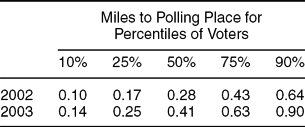
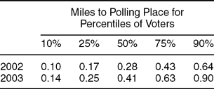
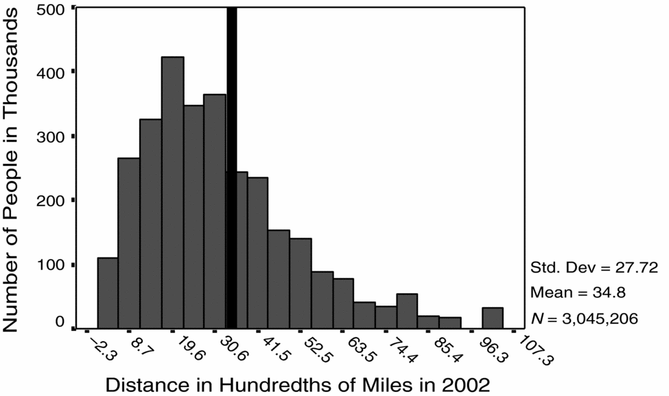
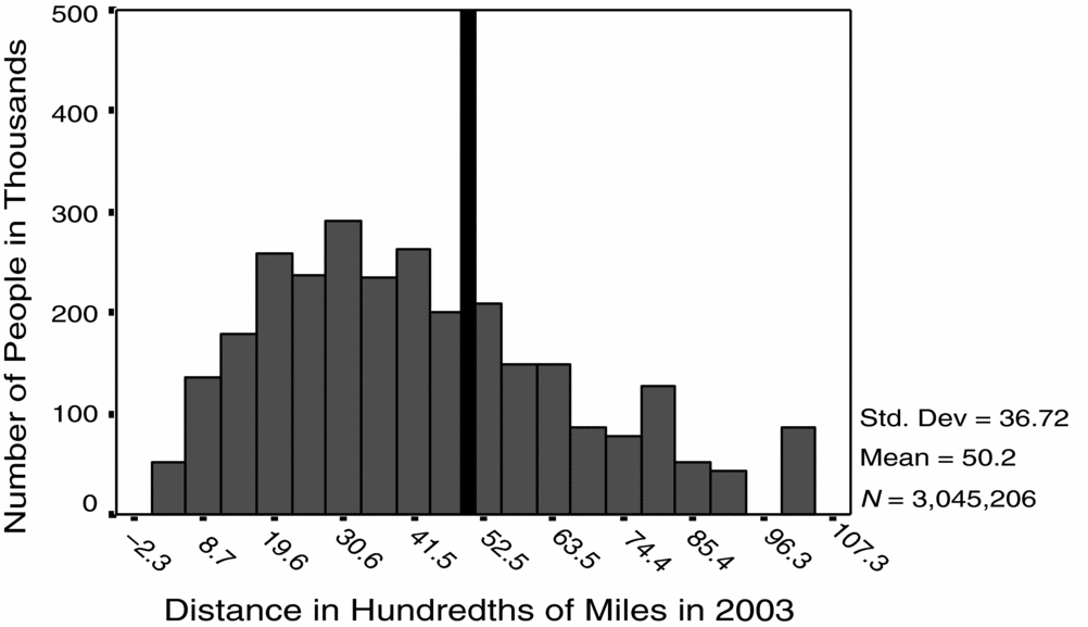
Not surprisingly, the 64% reduction in polling placesFootnote ⁸ in Los Angeles County between 2002 and 2003 increased the average distance that people had to travel to their polling places. Figures 1 and 2 present histograms for the distance that people traveled to their polling places in 2002 and 2003 among the 3,045,206 for whom we have geocoded addresses. Note that there is a clear shift to the right in 2003, with the average distance going from 0.348 miles to 0.502 miles—a mean increase of 0.154 miles, or 44.3%. In addition, the percentiles of the distribution shifted as shown in Table 1, and the median went from 0.28 to 0.41—a change of 0.13 miles, or about a 46% increase. In effect, the 25th percentile of voters in 2003 had to go about the same distance as the 50th percentile in 2002, and the 75th percentile in 2003 had to go about the same distance as the 90th percentile in 2002.

TABLE 1.

Average Distance to Polling Place in 2002 and 2003

N = 3,045,206.

FIGURE 1.

Distance to Polling Place in 2002

FIGURE 2.

Distance to Polling Place in 2003

Were Polling Places Changed Randomly? If polling places were truly changed randomly in 2003, then the 2002 characteristics of the treatment and control groups should be statistically indistinguishable from one another. Specifically, the proportion of registered voters turning out at the polls, voting absentee, and not voting should be the same. Using an estimation technique that takes into account the fact that assignment to treatment or control occurred on the basis of 9,275 registration precincts (voting precincts are pieced together from these smaller registration precincts), we find tiny differences in turnout in 2002 on the order of one tenth to four tenths of a percentage point, and only one of the measures for turnout differences (for absentee voting) is statistically significant at even the 0.05 level.Footnote ⁹ Although these turnout differences are extremely small, they are large enough compared to the size of our ultimate results (which are on the order of one to three percentage points) to suggest that it might be worth correcting for them.

Moreover, there were other differences as well. Consider distance to the polling place in 2002. Those who had their polling place changed in 2003 had to go an average distance of 0.354 miles in 2002, whereas those who did not have their polling place changed had to go only 0.320 miles—a difference of 0.034 miles, which is highly statistically significant, although substantively rather small—about 60 yards. Even though it seems unlikely that initial differences in distance to the polling place are confounding our results, one of our theoretical goals is to learn about the impact of changes in polling place distance on voting, and based on our theoretical model (see Appendix B), this impact might depend on people's past experience with distance to their polling place. Consequently, there is a theoretical argument for controlling for initial (2002) polling place distance.

Another important determinant of voting is age, and we have a reasonable year of birth for about 91.4% of the voters on the file. We find very small preexisting differences between the two groups (treatment and control) by age, but there are about 0.73% more people older than 60 years in the group that did not have its polling place changed.

The Assignment Process. These results demonstrate that the consolidation process was very nearly but not perfectly random. So what principles were used for the assignment of polling places? In the worst-case scenario, a highly partisan Registrar of Voters might change polling locations for precincts with large concentrations of partisans of one particular party, but this seems unlikely in California with its progressive tradition of choosing registrars based on their efficiency and effectiveness, not their partisan identification. It seems much more likely that a Registrar of Voters would change polling places to minimize the reduction in turnout that might be expected from such a change.Footnote ¹⁰ To do this, the registrar would need some theory about what affects voting turnout and some relevant data on the precincts. The voter registration file would provide the most useful data, and the theories would presumably be fairly simple—such as believing that past voting behavior predicts future voting behavior, travel distance matters, and age affects voting behavior. This simplifies the modeling process because it suggests that we probably have at hand most of the information that was used by the registrar in changing polling places.

The registrar might consolidate precincts with greater fractions of absentee voters because changing the polling place of absentee voters has little to no impact on their turnout.Footnote ¹¹ The registrar might be less likely to consolidate precincts with more elderly voters, especially if they had large numbers of polling place voters. The registrar might be more likely to consolidate those precincts with fewer people than those with more people because fewer voters would be discomfited by changing their location. Finally, the decision to change a polling place might take into account 2002 distance to the polling place for the voters in a precinct. The registrar might try to reorganize polling places that are on average far away from voters in such a way as to minimize increases in distance. This presumably requires changing more of these polling places. These measures would tend to reduce public complaints about the process, something all service agencies seek to minimize, if not for the pleasure of performing their functions well, then merely due to self-interest.

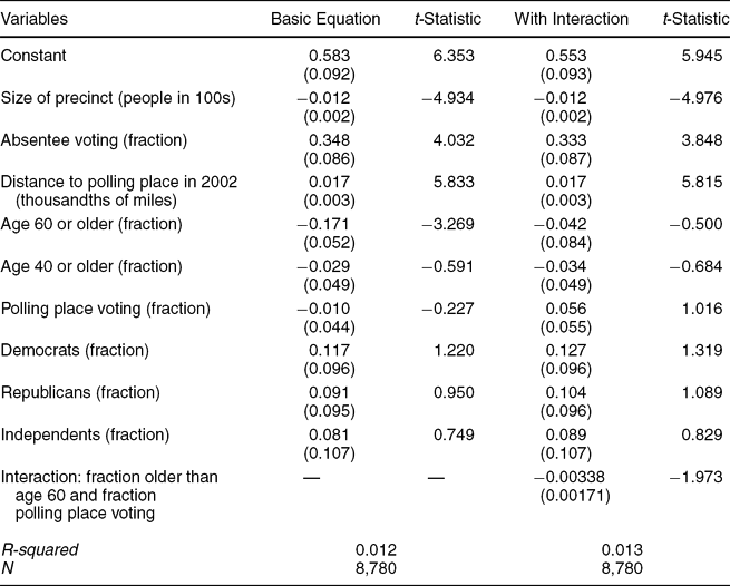
Following the classic works by Heckman (Reference Heckman1979) and Achen (Reference Achen1986), the registrar's assignment (or selection) process is modeled by regressing a binary variable for “treatment” or “control” on the covariates believed to be important for the selection process. Because the decision was made by registration precincts, we use these as the unit of analysis. Hence, those variables related to individual characteristics or distance to the polling place are averages for those in the registration precinct.Footnote ¹² To simplify the process of interpreting the regression, we present results from a linear regression (or a linear probability model without a Goldberger correction), although a logistic or probit regression yields exactly the same pattern.

Table 2 presents the results for two regressions of the treatment variable on the four factors that we believed would be important for assignment and some others that we believed would not be. First, the number of people in the registration precinct matters. Those precincts with more people are less likely to have their polling place changed. Thus, a relatively large registration precinct of 500 people (at the 75th percentile in size) is about 5% less likely to have its polling place changed than a small registration precinct of 100 people (at the 25th percentile). Second, a registration precinct with a relatively high level of absentee voting at 12% (at the 75th percentile) is about 2% more likely to have its polling place changed than a registration precinct with only 6% absentee (at the 25th percentile). Third, a registration precinct in which its voters have to go one quarter mile more to get to their polling place has a 4% greater chance of having its polling place changed. Fourth, a registration precinct that goes from 14% older than 60 years (the 25th percentile) to 24% older than 60 years (the 75th percentile) decreases its chances of having its polling place changed by almost 2%. However, the fraction of people ages 40 to 59 years; the fraction of polling place voters; and the fraction of Democrats, Republicans, or Independents do not affect the selection probability. The second column of regression coefficients adds another fact—it is not the percent of those older than 60 years that matters so much as its interaction with the percent who vote at the polling place.

TABLE 2.

Selection Regression for Assignment of Registration Precincts

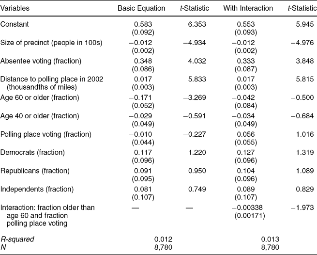
Despite these findings, perhaps the most important feature of this regression is that it explains very little of the selection process—the R squared is only 0.012, meaning that only about 1.2% of the variance is explained. If the variables included in the regression are, in fact, the only ones that affected the assignment of polling places, then this small R squared indicates that the assignment was nearly random. Nevertheless, the regression suggests that some strategies were used to mitigate the adverse impacts of changed polling places so we should seek an approach that will allow us to correct for this modest but still possibly significant nonrandom assignment of precincts to control or treatment status.

STATISTICAL MATCHING RESULTS

We correct for nonrandom assignment using statistical matching (Imbens Reference Imbens2004; Morgan and Harding Reference Morgan and Harding2006; Rosenbaum Reference Rosenbaum2002). Matching deals with the fundamental problem of causal inference, the fact that we can only observe each unit in either the treated or control condition, but not both, by taking each observed unit and matching it with one or more other similar observed units that received the opposite treatment. Thus, for a unit that received the treatment, we find a unit with similar characteristics that did not receive the treatment. We then use this unit as the imputed control for the treated unit. The trick, of course, is to match on the right characteristics, and this must be done to satisfy what is called the “conditional independence assumption” or the “unconfoundedness” assumption (Holland Reference Holland1986; Neyman Reference Neyman, Dabrowska and Speed1923; Rubin Reference Rubin1974). In our case, the obvious matching variables are those that are significant in our selection equation. The success of the matching can be evaluated by how well other variables that might be considered important are balanced in the matched data. That is, the extent to which we have similar distributions of these variables in the treatment and control cases.

Matching Variables. What should we choose as our matching variables? Should we match on all four significant factors (2002 turnout, age, size of precinct, and distance to polling place in 2002) in our selection equation? Matching is only necessary for those variables that might be correlated with 2003 turnout. There are very strong reasons for expecting 2002 turnout behavior (Gerber, Green, and Shachar Reference Gerber, Green and Shachar2003) and age (Miller and Shanks Reference Miller and Shanks1996, chapter 3) to affect turnout so we match on it. The size of a precinct is another matter. A direct relationship between the number of registered voters in a precinct in which someone resides and those factors that have a causal impact on individual turnout seems very unlikely, so we do not match on size of precinct.Footnote ¹³ It is not immediately obvious that 2002 distance to the polling place might affect 2003 turnout; however, in simple bivariate regressions, for each one tenth of a mile increase in distance to the polling place in 2002, polling place voting in 2002 decreased by about 0.27% and absentee voting in 2002 increased by about 0.25%. These results strongly suggest that 2002 distance to the polling place might have an impact on voting in 2003. Hence, even though there was very good initial balance in 2002 distance to the polling place, we nevertheless matched on this distance because it was statistically significant in our selection equation.

There are also other reasons for matching on 2002 distance to the polling place. Among those whose polling places were changed, the correlation between the change in polling place distance between 2002 and 2003 (presumably a measure of the strength of the “treatment”) and a person's polling place distance in 2002 is −0.293, even though the correlation between having your polling place changed in 2003 and your polling place distance in 2002 is much smaller at 0.050. That is, whether your polling place was changed in 2003 did not have much to do with how far you had to go to your polling place in 2002, but once the decision was made to change your polling place, the change in distance was strongly (negatively) related to your 2002 polling place distance. It appears as if efforts were made to reduce the distance to polling places in 2003 for those who had appreciable distances to go in 2002.Footnote ¹⁴

Consequently, another reason to match on 2002 distances to polling places is that even though the treatment and control groups were initially balanced with respect to this distance, the putative treatment strengths (i.e., the changes in distance to the polling place between 2002 and 2003) differed by this distance. If we want to determine the impact of different treatment strengths, then we must match on 2002 distance to the polling place. Moreover, there is still another reason for considering 2002 distance to polling place. Perhaps distance to polling place in 2002 interacts with the treatment to make it more or less efficacious. Thus, even if distance to polling place in 2002 were unrelated to turnout in 2003, failing to control for it would lead to a missed opportunity—we would not learn whether there is an interaction between this variable and the effects of the treatment.Footnote ¹⁵

To facilitate matching cases with respect to people's turnout behavior in 2002, their age, and their distance to the polling place in 2002, we put each variable into categories. Past turnout is in three categories (voted at polling place, voted absentee, or did not vote). We combined some age groups (starting with those 61 years or older) to get 53 relatively equal-size categories with an average size of 52,486.Footnote ¹⁶ We created 74 categories for distance to the polling place in 2002, with the number of cases in each category ranging from 12,743 to 66,800. In most cases, an exact match required that the matched observation have a distance within plus or minus 0.01 miles.Footnote ¹⁷ There were 11,766 potential matching categories (3 × 53 × 74), and there were 2,781,895 observations with data on all three variables. All but 14 of these categories had both treatment and control observations, which reduced the number of observations by 133 to 2,781,762 observations. In the results reported here, we matched using a modification of Sekhon's “matching” package for R (Mebane and Sekhon Reference Mebane and Sekhon1998; Sekhon n.d). To generate average treatment effects, observations were paired with all exact matches across “experimental” conditions to produce 513,934,138 matched pairs. The modified program produced standard errors, which took into account the fact that “randomization” was across registration precincts and not individuals.

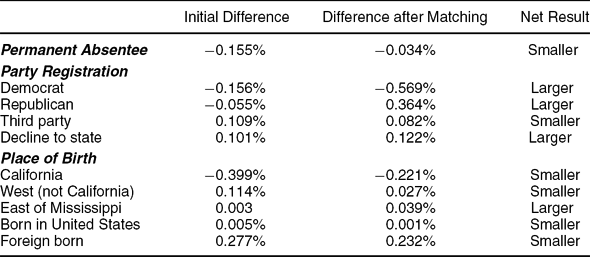
Matching Balance. Before presenting the results, it is useful to consider the degree to which the data are “balanced” on other important variables that might be associated with turnout. The matching ensures that the data are balanced with respect to turnout in 2002, age, and distance to polling place in 2002, but does it also create balance on other variables? We consider three variables that were reasonably complete on the voting files: permanent absentee status, party registration, and place of birth. About 4.4% of the sample had chosen to use absentee ballots “permanently,” and 71.5% of them actually voted absentee in 2002, whereas 10.2% of them voted at their polling place. About 52% registered as Democrats, 28% as Republicans, 16% as “decline to state,” and 5% with other parties. We coded birthplaces into five categories: California (41%), East of the Mississippi River (19%), West of the Mississippi River but not California (10%), foreign born (29%), and United States born (1.2%).

Table 3 presents the balance results. We present both initial differences (treatment minus control) in percentages and the final differences after matching. The initial differences in party registration show that there was no (successful) effort to change polling places so as to affect the partisans of one party more than another. There was a tiny bit more of both Democrats and Republicans in the control than in the treatment group, but the net difference was 0.101%, or only about 1,800 voters. Of these only, about two thirds had their polling place changed, and at most, only about 2% did not vote—for a puny impact of about 24 voters lost for the Democrats or a minuscule 0.001% of total partisan voters.

TABLE 3.

Changes in Balance Due to Matching (Treatment Minus Control)

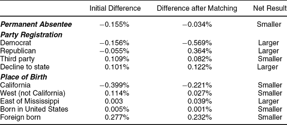
For the rest of the results, it does not make a great deal of sense to present t-statistics because the large sample ensures that most of these differences are statistically significant. Rather, we focus on their size. Of the 10 differences, 6 of them are smaller after matching, 1 is about the same (for “decline to state”), and 3 are bigger (for “born in the East,” Democrat, and Republican). The two largest differences in absolute value are for Democrats (0.57%) and Republicans (−0.36%), but most are much smaller. The partisan difference might be considered a problem, but what seems to matter for turnout is major party membership versus “decline to state” or third-party membership. Those registered with the two major parties turned out at rates of 65.5% in 2002 in Los Angeles (Republicans) and 59.3% (Democrats), whereas those not registered with the major parties turned out at 47.2% (decline to state) and 46.3% (third parties)—so partisans of the major parties voted at rates that were about 15 percentage points higher than others. Thus, the important figure is the net reduction in partisans in the treatment group due to the imbalance. This figure is about 0.20%, which is the population-weighted difference of the weighted average of −0.569 and 0.364 and the weighted average of 0.082 and 0.122. Thus, we would expect that the treatment group would have lower turnout of about 0.15 * 0.20% = 0.03%, which is only about one thirtieth of the smallest effect sizes of about 1.00% that we find.

Matching Results. Table 4 presents the results for the three 2003 turnout variables after matching on turnout in 2002, distance to polling place in 2002, and age. The first column reports the raw results without matching. The second column reports results from matching. The decline of 3.03% in polling place voting is similar to the unadjusted results, but nonvoting appears to be much higher at 1.85% and absentee voting much lower at 1.18%.Footnote ¹⁸ These results most likely reflect the mitigating efforts taken by the Registrar of Voters. The matching results for nonvoting can be thought of as what would have occurred had the registrar not exerted any efforts to mitigate the impact of changing polling places, and the raw results can be considered the smaller decline in nonvoting that actually occurred. The relatively small difference in nonvoting between the unadjusted and matching results—only 0.379 percentage points—suggests the difficulty of overcoming the problems of consolidating precincts. The third and fourth columns present two estimates of t statistics. The third column presents the t statistics computed by ignoring the fact that blocs of voters in registration precincts were assigned to the “treatment” or “control” condition en masse. The fourth column presents t statistics computed by making an adjustment to the matching estimator to simulate the HLM method used previously in this article. These t statistics are somewhat smaller in absolute value than those in the third column, but they are still exceptionally large.Footnote ¹⁹

TABLE 4.

Outcome Estimates: Unadjusted and Matched

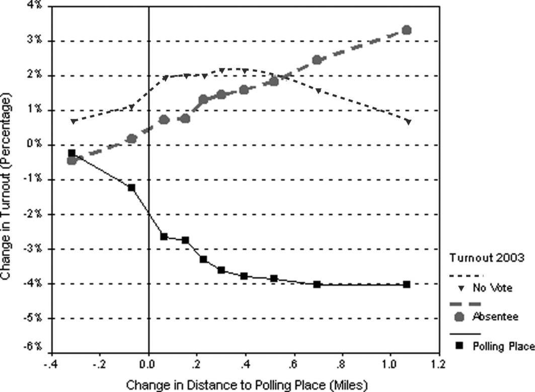
Impact of Changes in Distance to Polling Place. We can use matching methods to disentangle search and transportation effects by plotting the difference in turnout between those who had their polling place moved and those who did not by the various amounts of change in distance to the polling place between 2002 and 2003. Figure 3 presents polling place turnout, absentee turnout, and nonvoting estimated over a range of possible changes in distance to the polling place. The data for Figure 3 were obtained by sorting the treatment group into 10 approximately equal-size groups (ranging from 99,753 to 267,793 people), depending on the change in their distance to their polling place between 2002 and 2003. Each group was assigned the median value of the change in polling place distance for those in the group (thus yielding values of −0.3181, −0.0714, 0.0624, 0.1552, 0.2253, 0.3034, 0.3959, 0.5175, 0.6974, and 1.0644 miles). We can think of these as different “doses” of the change in distance to polling place treatment. For each dose level, we match the treatment and control groups by 2002 turnout, 2002 distance to the polling place, and age. Within each dose level, we compared turnout for those in the treatment group who got that dose (for a given set of matching characteristics) with all those in the control group with those matching characteristics. These estimates of the effect for each dose are then added up across the matching groups to obtain the average treatment effect for the dose. The standard errors for the points on these lines are approximately 0.18% so that a 95% confidence interval would be the estimates plus or minus approximately 0.36%. Note that the veracity of the estimates depends on the assumption that the doses are essentially randomly assigned conditional on the matching characteristics. This assumption seems more likely to be true because we matched on initial distance to the polling place in 2002 to deal with the fact that the amount of change possible is obviously correlated with the “room for change” given the initial distance to the polling place.

FIGURE 3.

Search and Transportation Effects

As we would expect, voting at the polling place (the solid line) decreases with an increasing value for the change in distance to the polling place. Moreover, when the change in distance is zero, we can estimate the pure search effect of about −1.8%, and the slope of the line, about −0.50% per one tenth of a mile for the part of the curve between −0.40 and 0.40 miles and almost zero thereafter, indicates the transportation effect. Part of this reduction in turnout was alleviated by an increase in absentee voting (the dashed line), with the pure information effect of 0.50% and the transportation effect of about 0.25% throughout the range. Thus, just by having a polling place changed, polling place voting decreases by 1.8%, and 0.5% is replaced with absentee voting for a net decrease in voting of 1.3% (see the dotted “no vote” line). For each one tenth of a mile increase in distance up to 0.4 of a mile, polling place voting decreases by 0.50%, and about half of this (0.25%) is supplanted by absentee voting for a net reduction of 0.25% per one tenth of a mile up to 0.40 of a mile. Beyond four tenths of a mile, increased absentee voting actually decreases the amount of nonvoting to perhaps 1%. Figure 3 shows that both search and transportation effects matter.

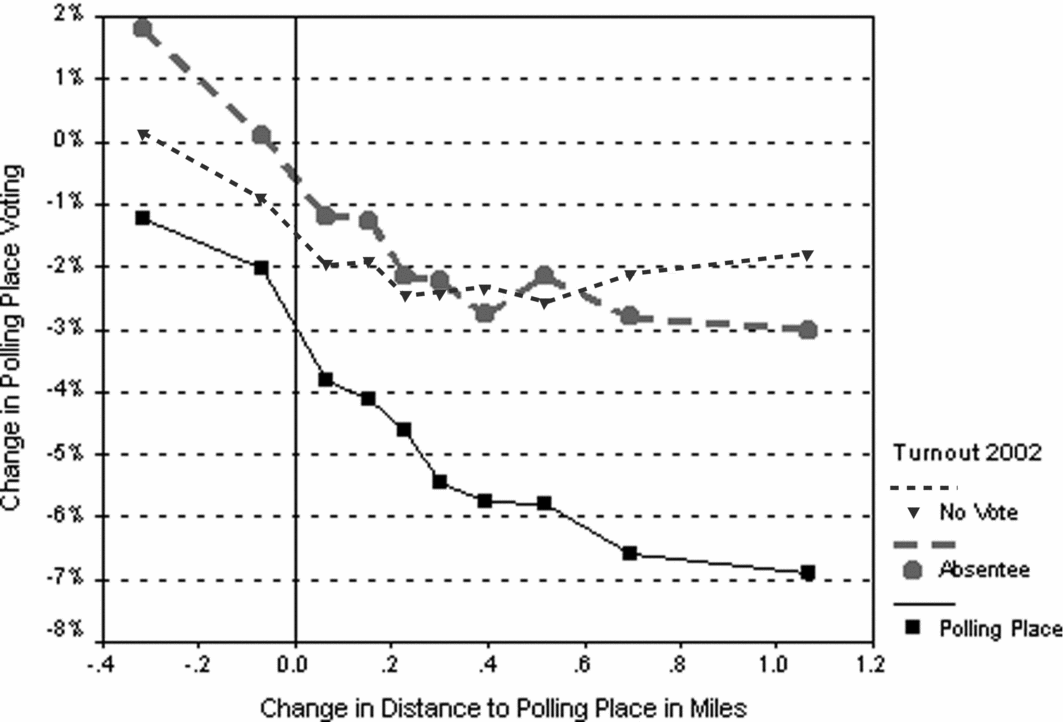
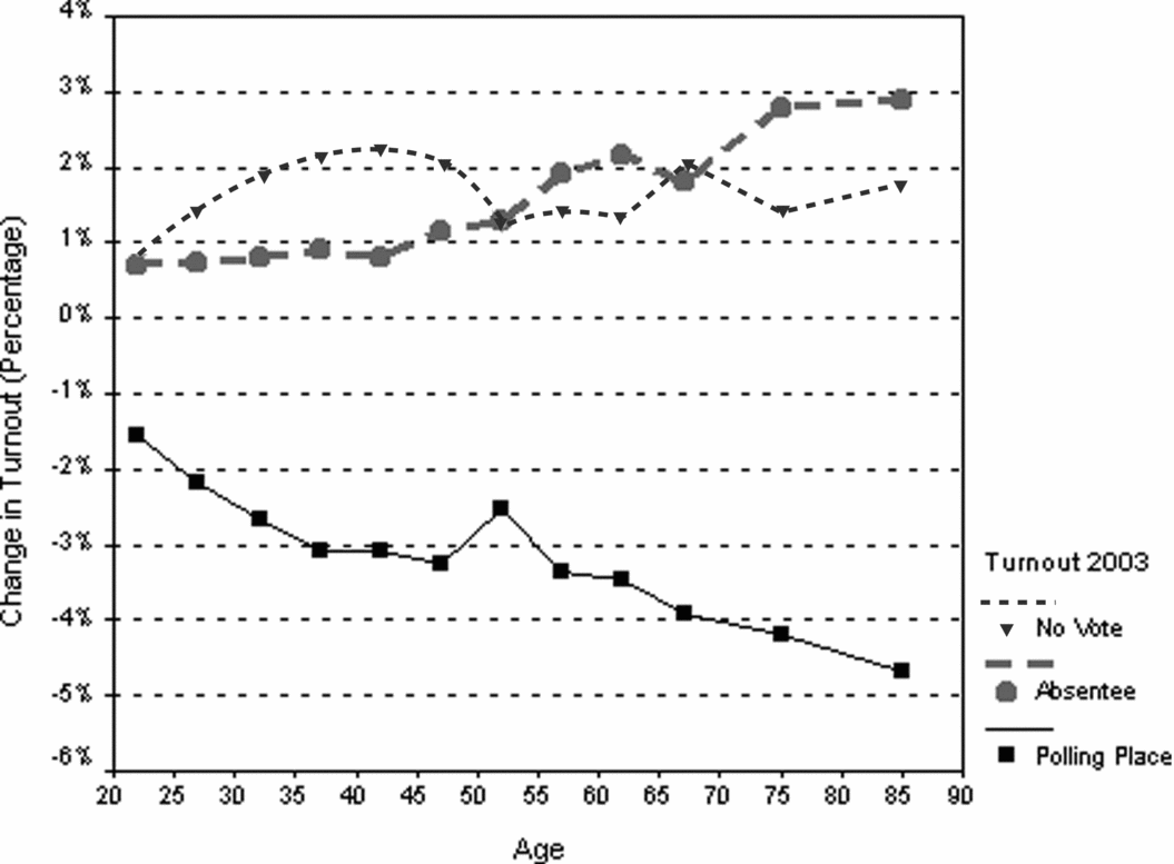
It also seems likely that the impact of changing polling places in 2003 varies by turnout behavior in 2002, a voter's age, and distance to the polling place in 2002. We consider each of these in turn. Figure 4 shows the impact on polling place voting in 2003 by type of turnout in 2002. The biggest declines in polling place turnout in 2003 are for those who voted at their polling place in 2002 (see the solid line). There is also a substantial impact on absentee voters (see the dashed line), and, as we might expect, very little impact on those who did not vote in 2002. Moving on to the impacts of age, Figure 5 shows that older voters reduce their polling place voting much more than younger voters (see the solid line), but they also substitute absentee voting (the dashed line) at a much higher rate. The net result is similar rates of increased nonvoting (the dotted line) across all age groups.Footnote ²⁰

FIGURE 4.

Change in Polling Place Voting in 2003 by Change in Polling Place Distance by Turnout in 2002

FIGURE 5.

Change in Turnout in 2003 by Age

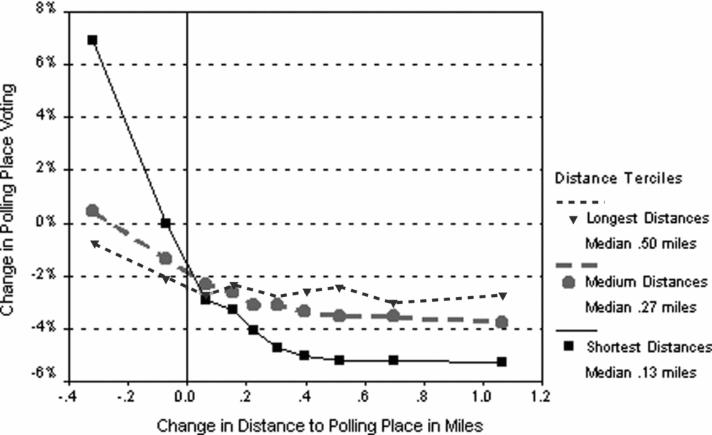
Finally, consider how initial distance to the polling place in 2002 affects the relationship between turnout and the change in polling place distance between 2002 and 2003. Figure 6 plots polling place turnout by change in distance to polling place for three different initial distances to the polling place in 2002. The solid line is for initial distances of zero to 0.2 of a mile (about 33% of the sample with a median of 0.13 mile), the dashed line is for distances of 0.21 to 0.37 miles (about 35% of the sample with a median of 0.27 mile), and the dotted line is for distances of 0.38 to several miles (about 33% of the sample with a median of 0.50). There is a clear impact with the greatest effects (i.e., the steepest lines) for the shortest initial distances in 2002.

FIGURE 6.

Change in Polling Place Voting in 2003 by Change in Polling Place Distance in 2003 by 2002 Distance to Polling Place in Terciles

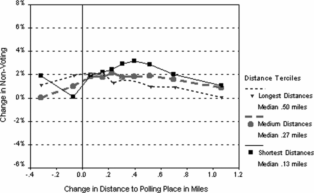
Common sense suggests that nonvoting should also be affected by changes in distance to the polling place. It seems reasonable that people who voted at their polling place in the past and who find absentee voting onerous will simply decide not to vote when confronted with a polling place that is much farther away in 2003. Yet, Figure 3 suggests that there is, at best, only a slight relationship between nonvoting and distance to the polling place, and Figure 7 shows that there is even less evidence for an impact of an increase on distance to the polling place on nonvoting after controlling for initial (2002) distance to the polling place. There appears to be no relationship between nonvoting and change in distance to the polling place regardless of the initial distance. Statistical estimates in Appendix B confirm this result.

FIGURE 7.

Change in Non-Voting in 2003 by Change in Polling Place Distance in 2003 by 2002 Distance to Polling Place in Terciles

Summary of Results. People appear to make decisions in a two-step, “boundedly rational” (Conlisk Reference Conlisk1996) process. They initially decide whether to vote based on just the increased search costs imposed by changed polling places. Then, once they have decided to vote, they decide whether to vote at the polling place or absentee by also considering changed distances (see Appendix B for more discussion of this process.)

These results demonstrate the importance of convenience, habituation, and learning for voting. Changes in polling places and increased distances to polling places change turnout behavior due to increased inconvenience. Because they are most discomfited by changes, older voters and voters used to voting at their polling places reduce their polling place voting the most when their polling place is changed. But those people who are habituated to going long distances to their polling place are less affected by increased distances to polling places, and older people (whom we can presume have learned about the voting system) substitute absentee voting for polling place voting.

These results lead us back to the question with which we began: how does distance matter? Certainly, a change in polling place distance matters because our analysis passes the tests for a reliable causal inference: a change of polling places occurred for some people in Los Angeles (i.e., there was a manipulation of the putative cause); we had a real control group; we did our best to control for confounders; and we found significant effects. But what does it mean, for example, that the size of this change is conditioned on polling place distance in 2002? What does polling place distance in 2002 actually measure? Does it stand for some unobserved heterogeneity that is not captured by our matching variables? What could cause this heterogeneity? Is it correct to say that some people are generally more used to long trips than others so that they are less affected by changes in their polling place location? Or is something else going on? These are questions for future research.

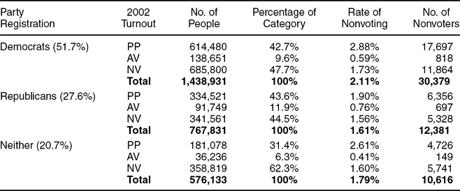
Partisan Impacts. Increasing costs certainly affect turnout, but do they have partisan implications as well? In Table 5, we estimate the increase in the nonvoting rate from the changing of polling places separately by party registration (Democratic, Republican, and Neither) and polling place in 2002. The rates are estimated after matching on age and 2002 distance to the polling place. We find that the increase in nonvoting rates for Democrats is higher than for Republicans for those who voted at the polling place (PP) in 2002 (2.88% to 1.90%) and for those who did not vote (NV) in 2002 (1.73% and 1.56%). These two groups account for 90.4% of the Democrats and 88.1% of the Republicans. Hence, even though the increase in nonvoting rate is slightly higher for Republicans who voted absentee in 2002 than for Democrats who voted in absentee in 2002 (0.76% compared to 0.59%), the overall increase in nonvoting rate is higher among the Democrats (2.11%) than among the Republicans (1.61%).

TABLE 5.

Estimation of Increase in Nonvoters Due to Changes in Polling Place by Party Registration and 2002 Vote

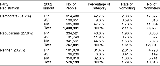
We can convert these nonvoting rates into the number of voters who did not turn out. The sixth (and last) column of each of the three party registration categories estimates the number of nonvoters by applying the rate of nonvoting (in the fifth column) to the number of voters in that group (the third column) to get the number of nonvoters. This gives 30,379 for the Democrats and 12,381 for the Republicans, for a difference of 17,998. This difference is actually too high because it assumes that the changing of voting places affected everybody when, in fact, it only affects about two thirds of the population; thus, a reasonable estimate of the ceiling of potential Democratic votes lost is 12,000, which assumes that voters reliably vote for the party in which they are registered.Footnote ²¹

This can be broken into two pieces. Because Los Angeles has more Democratic registration than Republican, a constant reduction in turnout across the two party groups of 1.94% (the weighted average of 2.11% and 1.61%) affects more Democrats than Republicans—about 8,700 more. This reduction does not affect the relative ratio of Democrats to Republicans within Los Angeles County, but it does mean that fewer Democrats voted in Los Angeles County than if there had been no changes in polling places. If in California only Los Angeles disrupted its voters in this way, then Democrats would be less represented than if no disruptions had taken place. Second, because Democrats reduce their voting by 2.11% compared to Republicans, who reduce their voting by only 1.61%, the net loss to Democrats is another 3,300 votes. This changes the partisan margin by about 0.22%. This is a very small figure, but about one in two hundred contested House elections have a margin this size.Footnote ²² Hence, changing polling place locations could affect an election, even when the registrar was trying mightily not to manipulate polling places in a partisan manner. Moreover, substantial manipulation might be possible if there were intent to do so by changing polling places only in those places that leaned one way.

CONCLUSION

Although the 2003 changes in polling places is not a perfect natural experiment, it is about as close as we come with observational data. Consequently, it provides us with a strong inference that the changes in Los Angeles County reduced turnout by a substantial 1.85% in the precincts where the polling location was changed. We also find that voting at the polling place decreases even more, by 3.03%, but that an absentee voting increase of 1.18% makes up for some of this reduction. In addition, we find that the substitution of absentee voting for a reduction in polling place voting is greatest among people of middle age and older, whereas younger people are more inclined to simply not vote at all.

Change in polling place location had the two effects we expected: a transportation effect resulting from the change in distance to the polling place and a search effect resulting from the costs of finding and going to a new polling place. About 60% of the 3.03% reduction in turnout at the polling place is due to the search effect (of about 1.80%), and the impact of the search effect is about two and one-half times larger than the transportation effect for the average person who experienced an increased distance to the polling place of about one sixth of a mile. The two effects were roughly equal for someone who had an increased distance to the polling place of about a mile. The overall reduction in not voting of about 1.85% is almost entirely due to the search effect (about 1.4%) because the decision not to vote appears to be essentially unaffected by the distance to the polling place. People make a decision about whether to vote based on the increased search costs from having their polling place moved, and if they decide to vote, they choose absentee or polling place voting based on both search and travel costs. This result implies that for those advocating larger, more economical precincts, if absentee ballots are as easy to come by as in California's “no excuse needed” system, then it seems that the increased travel costs will not seriously deter voting, although switching to a new system may impose substantial search costs that will at least temporarily reduce overall turnout. Finally, partisan effects are small enough that they can probably be ignored when polling places are essentially changed randomly, as in Los Angeles, but they are large enough that they could be used by an unscrupulous politician or registrar to manipulate an election.

APPENDIX A: MATCHING AND CLEANING OF DATA SETS

The data acquired for this article came from the Los Angeles County Registrar-Recorder/County Clerk. The voter data were obtained routinely; the polling place data less so. Individual-level voter data include the voter's name, registration precinct, residential address, mailing address, phone, party registration, sex, birthdate, birthplace, date of registration, date of last transaction, permanent absentee voter status, and turnout records (in-person voting, absentee voting, or abstention), along with several fields of identifying information and other miscellaneous data. Some of these data are incomplete. For example, dates and places of birth are missing in many cases, and sex is missing more often than not, although it can sometimes be inferred from the title field (Mr., Mrs., Miss). Still other pieces of data are obviously incorrect, such as an improbably large cohort of people born in 1900, as well as even “older” people born in the eighteenth and nineteenth centuries. We made a decision to code any birthdate prior to the year 1901 as missing. However, the critical data of precinct and turnout are always present.

Typically, the registrar maintains official records of past polling places in hard copy only. These records include polling place precincts, addresses, and descriptions (residence, business, church, school, etc.). Although data from 2003 turned out to be available electronically via a stroke of luck, data from 2002 had to be scanned in using optical character recognition software, and then reviewed line by line for correctness. We are grateful for the assistance of several colleagues at UC DATA and the Survey Research Center in executing this technically challenging and labor-intensive task, including Iris Hui, Ilona Einowski, Jon Stiles, Eva Seto, Lyn Civitello, Amy Kimball, Ricardo Gutierrez, Virginia Nee, and Alexander Theodoridis. We are also grateful to Conor M. Dowling and Cynthia M. Van Maanen at Binghamton University.

We then had to match each voter to their polling place for both 2002 and 2003. This was a challenge because the precincts reported for the voters were at a different level of aggregation than those reported for the polling place. Voters were associated with their registration precincts. Polling places were associated with their polling place precinct, which is composed of one or more (often many more) registration precincts. We needed to acquire “crosswalk” data to merge the two files so that each voter could be associated with a polling place precinct and its corresponding address. We obtained these data from both the Los Angeles County Registrar itself and from Karin McDonald of the Statewide Database at the Institute of Governmental Studies; we are grateful to both.

Having created complete files for 2002 and 2003, the final step was to match voters from the two years and look at voting behavior changes between 2002 and 2003, contingent on whether one's polling place was moved. We used the unique identifier Voter ID to match voters from both years; approximately 3% were not matched, probably due to normal churning (residential moving, mortality, etc.) in the electorate.

APPENDIX B: THEORY

Our model considers how the costs and benefits of voting are related to polling place, absentee, and nonvoting. The (utility) costs of voting at the polling place are represented by c^p (these costs consist of the sum of search and transportation costs) and the costs of voting absentee by c^a. The benefits of voting are represented by b. Footnote ²³ Then the utility U_i^p that person i gets from polling place voting p will be the net benefits b_i − c_i^p for voting at the polling place. The utility U_i^a for voting absentee will be the net benefits b_i − c_i^a for voting absentee, and the utility U_iⁿ for not voting will be 0.Footnote ²⁴ The person will maximize his or her welfare by voting at the polling place (p_i = 1) if the net benefit of voting at the polls is greater than zero (b_i − c_i^p > 0) and the net benefit of voting at the polls exceeds the net benefits of absentee voting (b_i − c_i^p > b_i − c_i^a). The person will vote absentee if the net benefits of absentee voting are positive (b_i − c_i^a > 0) and the net benefits of absentee voting are greater than the net benefits of voting at the polls (b_i − c_i^a > b_i − c_i^p). Finally, the person will not vote if the (zero) net benefits of not voting are greater than the net benefits of voting at the polls (0 > b_i − c_i^p) and the net benefits of voting absentee (0 > b_i − c_i^a).

If we think of b_i, c_i^p, and c_i^a as realizations of random variables b, c^p, and c^a with a trivariate probability distribution that describes the voting population, then the proportion of people voting at the polls is equal to the following, where we have used capital letters to represent proportions:

(1)

$\begin{eqnarray} P = {\rm Prob}(p = 1) &=& {\rm Prob}\!\left(U_i ^p>U_i ^a \,{\rm and}\,U_i ^p>U_i ^n\right)\nonumber \\ & =& {\rm Prob}(b - c^p>b - c^a \,{\rm and}\,b - c^p>0) \nonumber\\ &=& {\rm Prob}(c^a>c^p \,{\rm and}\,b>c^p). \end{eqnarray}$

We get similar results for the proportion of people voting absentee:

(2)

$\begin{eqnarray} A = {\rm Prob}(a = 1) & = & {\rm Prob}\!\left(U_i ^a>U_i ^p \,{\rm and}\,U_i ^a>U_i ^n \right)\nonumber \\ &=& {\rm Prob}(b - c^a>b - c^p \,{\rm and}\,b - c^a>0)\nonumber\\ & = & {\rm Prob}(c^p>c^a \,{\rm and}\,b>c^a). \end{eqnarray}$

For the proportion of people not voting:

(3)

$\begin{eqnarray} N = {\rm Prob}(n = 1) & = & {\rm Prob}\!\left(U_i ^n>U_i ^p \,{\rm and}\,U_i ^n>U_i ^a \right)\nonumber \\ & = & {\rm Prob}(0>b - c^p \,{\rm and}\,0>b - c^a)\nonumber\\ & =& {\rm Prob}(c^p>b\,{\rm and}\,c^a>b). \end{eqnarray}$

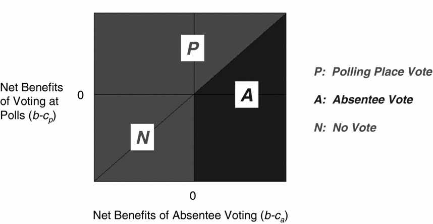
Figure B1 shows the formulas where we plot net benefits from polling place voting (b − c^p) versus net benefits from absentee voting (b − c^a). Each voter will be located somewhere in this space, depending on his or her values of b, c^p, and c^a. If a third dimension were added to this picture, then it could represent the density of each kind of voter. The diagonal on Figure B1 represents the place where net benefits from polling place voting equals the net benefits from absentee voting. The zero line on each axis represents the place where net benefits are zero. The nonvoters, indicated by N on the picture, are in the lower left-hand quadrant where net benefits are negative for both polling place and absentee voting (where 0 > b − c^p and 0 > b − c^a). The polling place voters, P, are above the diagonal (b − c^p > b − c^a) where the net benefits of polling place voting exceeds the net benefits of absentee voting, and they are above the zero net benefits line for polling place voting (b − c^p > 0). The absentee voters are below the diagonal (b − c^a > b − c^p) and to the right of zero net benefits for absentee voting (b − c^p > 0). The proportion in each of the three groups depends on the density of voters in each area. In the 2002 Los Angeles County governor's race, 55.1% of those registered did not vote, about 35.8% voted at the polling place, and 9.1% voted absentee, indicating that there were many voters in all three groups.

FIGURE B1.

Voter Decision Making

Now, consider what happens with precinct consolidation (and changes in polling places for some people) through the grouping of contiguous precincts. Assume that all precincts are grouped and that the additional cost of voting at the polling place due to grouping, c^g, is positive for everybody because of additional search and transportation costs. For voters, the cost of voting at the polling place increases from c^p to c^p + c^g. Then the proportions change to the following:

(4)

$\begin{eqnarray} P^* &=& {\rm Prob}(c^a>c^p + c^g \,{\rm and}\,b>c^p + c^g). \nonumber \\ A^* &=& {\rm Prob}(c^p + c^g>c^a \,{\rm and}\,b>c^a).\\ N^* &=& {\rm Prob}(c^p + c^g>b\,{\rm and}\,c^a>b). \nonumber \end{eqnarray}$

The first formula indicates that (as long as there are people at the margin for whom the change makes a difference) polling place voting will unequivocally decrease because c^g is greater than zero, and because there will be fewer people for whom the benefits of voting exceed the costs of polling place voting and for whom the costs of absentee voting are greater than the costs of polling place voting.

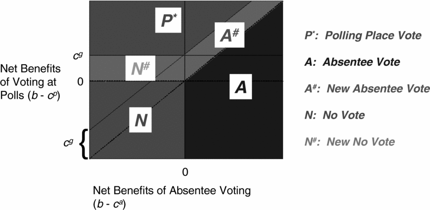
Figure B2 represents these changes by making shifts in two lines and by assuming that c^g is constant across all voters. First, the diagonal line in Figure B1 shifts upward by the amount c^g because the net benefits of polling place voting have decreased by that amount. Consequently, the net benefits of polling place voting will now only exceed or equal the net benefits of absentee voting for those people for whom their net benefits of polling place voting used to be c^g units or bigger than the net benefits of absentee voting. Second, the horizontal “zero” line shifts upward by c^g because the net benefits of polling place voting are now greater than zero only for those people for whom the benefits used to be at least c^g units bigger than zero. The resulting picture has two areas where voters move away from polling place voting. A^# designates people who turn to absentee voting. N^# designates people who no longer vote. Those who move into absentee voting will be people who always believed that the benefits of voting outweighed the costs of absentee voting but who formerly found it cheaper to vote at the polling place than through absentee ballots and now find it better to vote absentee because of the added cost, c^g, to polling place voting. Those who move into nonvoting will be those who never voted absentee (and will not now) because they calculate the costs of absentee voting to be greater than the benefits of voting, but they voted in the past because they found the benefits of voting at the polls to be greater than the costs of voting there. With the additional costs of voting at the polls, and with their long-standing belief that absentee voting costs more than the benefits of voting, they decide not to vote at all. The relative size of each group will depend on the size of c^g and the density of voters in these areas.

FIGURE B2.

Voter Decision Making with Shift in Cost of Polling Place Voting

Using Figures B1 and B2, we can write the proportions of each kind of voter (P*, A*, and N*) in the final situation in terms of the proportions in the original one and those who change their behavior:

(5)

$\begin{eqnarray} P^* = P - N^\# - A^\# \nonumber \\ A^* = A + A^\# \\ N^* = N + N^\# \nonumber \end{eqnarray}$

We can also write turnout as:

(6)

$\begin{equation} V^* = P^* + A^* = P + A - N^\# = V - N^\#\end{equation}$

This formula shows that the change in turnout (V* − V) will be the negative of the change in nonvoting (−N^#), and turnout will decrease less than polling place voting because some people will move away from polling place voting into absentee voting.Footnote ²⁵

These formulas can be used to show how changes in P, A, or N are related to changes in costs. Assume that c^g = δc^p, that is, c^g is a small change δc^p in the cost of polling place voting. Define the changes δP = P* − P, δA = A* − A, and δN = N* − N. We focus on changes in polling place voting. Consider the definition of the derivative (δP/δc^p ≡ P′), where P′ is the derivative of P(c^a, c^p, b) with respect to c^p evaluated at the point where the derivative is taken. Then after rearrangement, we write:

(7)

$\begin{equation} \udelta P = P^* - P = P'\udelta c^p.\end{equation}$

Consequently, observed changes in polling place voting (P* − P) are proportional to changes in costs δc^p with P′ as the “constant” of proportionality. The derivative P′ will be negative (because increases in c^p lead to decreases in polling place voting as shown previously). If we are considering a set of various changes in costs (i.e., different “experiments”) so that δc^p varies, then we can plot δP versus δc^p to determine the ceteris paribus impacts of costs as long as P′ is constant. If each “experiment” deals with a group of voters with a similar trivariate distribution of costs of absentee voting, benefits of voting, and costs of polling place voting (before any treatment), then P′ will be constant across experiments and meaningful comparisons can be made.

Consider how this applies to the changes in search and transportation costs that were made in Los Angeles. Assume that search (s) and transportation (t) costs enter linearly into the polling place cost function so that c^p = s + t. Further assume that transportation costs can be represented by a nonlinear function of the distance (d) to the polling place, t = d ^γ, where γ is positive so that transportation costs increase with distance.Footnote ²⁶ Then:

(8)

$\begin{equation} c^p = s + d^{\ugamma}\end{equation}$

At zero distance, s measures the search cost, which is assumed to be constant. If γ is less than one, then marginal costs diminish with increased distance. A change in costs can occur with a change in s or a change in d.

The impact of a change in s alone or d alone can be measured by P* − P as long as the changes are randomly assigned so that P represents the polling place voting of the “control” group and P* represents the polling place voting of the “treatment” group that gets the change. This might, however, give an incomplete picture of the impact of changes in d because the impact will vary significantly with the baseline value of d if the parameter γ is less than one, especially if it is less than about three-fourths. We can show this directly. For a change in d, we can write Equation (7) as:

(9)

$\begin{equation} \udelta P = P^* - P = P'(\udelta c^p/\udelta d)\udelta d.\end{equation}$

In this formula, P′ is as before (but evaluated at the current value of c^p) and the derivative (δc^p/δd) is:

(10)

$\begin{equation} (\udelta c^p/\udelta d) = \ugamma \,d^{\ugamma - 1}\end{equation}$

Consequently, we have that:

(11)

$\begin{equation} \udelta P = P^* - P = (\ugamma \,d^{\ugamma - 1})P'\udelta d.\end{equation}$

If γ is less than one, then the quantity in parentheses is much bigger for smaller distances than for larger ones (i.e., its size is inversely related to distance) so that the slope of a plot of δP versus δd will be much more negatively sloped (because of the sign of P′) for smaller distances than for bigger ones (assuming that the value of P′ stays about the same as these distances vary).Footnote ²⁷ Thus, a change in distance to one's polling place will matter much more for those who initially travel short distances to their polling place than those who travel long distances. As a result, although an experimental approach will give the correct “average effect,” it will miss the important variation in the impact of distance on nonvoting, which depends on the initial distance to the polls. Furthermore, in a nonexperimental situation, if the change in distance to the polls is correlated with the initial distance to the polls, then there could be bias in the estimates of the impact of changes in distance. This discussion implies that we should control initial distance to polling place in our analysis as well as other factors, even if initial distance to the polls is fairly well balanced initially between the experimental and treatment groups.

We can use this theory to get an equation for estimating the relationship between changes in polling place voting and changes in distance to the polling place. From Equation (8), we have the following when both search costs and distance to polling place changes:

(12)

$\begin{equation} \udelta c^p = \udelta s + \ugamma \,d^{\ugamma - 1} \,\udelta d\end{equation}$

Using this equation and Equation (7), we can write that:

(13)

$\begin{equation} \udelta P = P'\udelta s + P'\ugamma \,d^{\ugamma - 1} \udelta d.\end{equation}$

We might further assume that δs is some constant amount plus some amount that varies with observed characteristics such as age and unobserved characteristics ϵ:

(14)

$\begin{equation} \udelta s = \ualpha + \ubeta ({\rm Age}) + \uvarepsilon.\end{equation}$

Then we can write:

(15)

$\begin{equation} \udelta P = P'\ualpha + P'\ubeta (Age) + P'\ugamma \,d^{\ugamma - 1} \,\udelta d + \uvarepsilon.\end{equation}$

This equation can be estimated using nonlinear least squares. If Age is measured from voting age (so that a person who is 18 in 2002 has age zero), then the parameters can be interpreted as follows: P′α is the baseline search cost (in terms of decreased polling place voting) for a person of zero political age (i.e., 18) whose polling place is changed, but for whom the distance to his or her polling place does not change (δd = 0); P′β is the impact of aging one year; and P′γd ^γ−1 is the impact of a unit change in distance, which clearly depends on initial distance in 2002 (d) according to the parameter γ.Footnote ²⁸ If the exponent γ is less than one, then marginal costs diminish with increased distance.

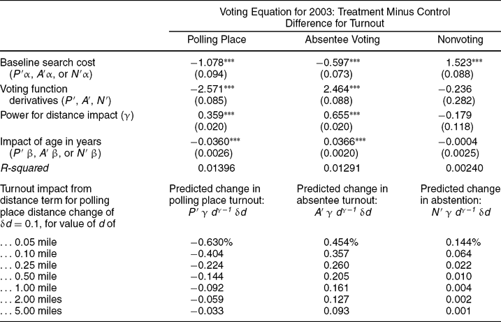
Table B1 presents estimates for the various parameters in nonlinear least squares fits to Equation (15) for the three outcomes of percentage changes in polling place voting, absentee voting, and nonvoting. Table B1 also presents some estimates of impacts for a one-tenth mile change in polling place distance, depending on various 2002 distances to the polling place. This provides a simple way to interpret terms such as (P′γd ^γ−1δd).

TABLE B1.

Summary of Impacts of Changing Polling Place Locations for Entire Sample

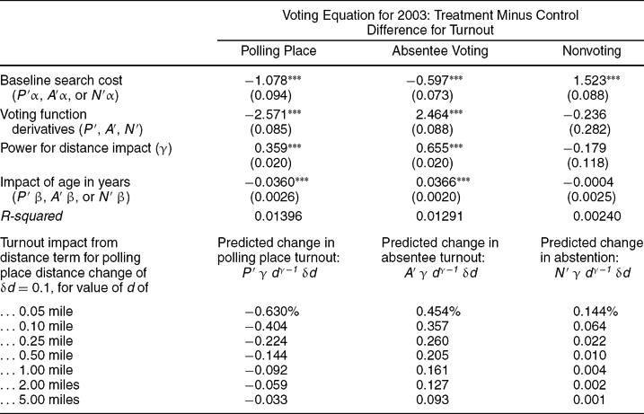
Dependent variables are measured in percentages, distances are measured in miles, and age is measured in years. *** Indicates coefficient is significant at .001 level.

It is important to understand what these estimates are and are not. If our conditional independence assumption holds, then our matching on age, distance to polling place in 2002, and voting status in 2002 amounts to stratifying our sample and then randomly assigning polling places within each strata. Consequently, we can determine the variations in the effects of the treatment across the different strata. However, these results should be interpreted very carefully. A negative coefficient for age, for example, means that changing polling places causes more nonvoting among older people than among younger people. It does not necessarily mean that a manipulation of age alone would decrease voting.

Table B1 provides some interesting results. Consider polling place voting. There was a one percentage point reduction in polling place voting simply due to search costs for a voter who was 18 in 2002. In addition, there was a substantial reduction in polling place voting due to age—about 0.036% for every year of age (or 0.36% for every 10 years of age) so that the average 47 year old voter had another 1% reduction due to search costs. The results for distance indicate that a one tenth of a mile increase in distance to the polling place in 2003 led to between a 0.63% to 0.03% reduction in polling place voting with the bigger effects for those who were used to their polling place being located nearby. (The γ parameter is clearly statistically different from zero and statistically less than one so that we would expect these distance effects.)

For absentee voting, there is a somewhat surprising negative value of −0.597% for baseline search costs, which indicates that 18-year-old voters in 2002 who had their polling place changed but who did not have the distance to their polling place changed actually reduced their absentee voting. In fact, a more careful treatment of age suggests that this unlikely result does not occur. If we use dummy variables for 10-year age periods, then we find that there is, as the age coefficient in Table B1 suggests, an increase in absentee voting with age, and among those in the lowest age bracket, there is essentially no increase in absentee voting due to a change in polling place. Thus, the negative value for baseline search costs is essentially due to a (slight) nonlinearity in the impact of age. In fact, the coefficient of 0.366% for age shows that aging 16 years from 18 to 34 brings search costs to zero. It is also worth noting that the decrease in polling place voting due to age in the first column is almost exactly balanced by the increase in absentee balloting due to age.

Changes in polling place distance operate in roughly opposite directions by decreasing polling place voting and increasing absentee voting. The values for the derivative of the voting functions are about equal and opposite, but the value for the power (γ) of the distance term differs so that the curves have different shapes. The chart at the bottom of Table B1 shows that for one tenth of a mile change in distance, the reduction in polling place voting is much steeper with initial distance to the polling place than is the increase in absentee voting.

Finally, consider nonvoting. There is a large baseline effect of 1.523%, and there is no increase (or decrease) in nonvoting because of age. The most interesting result is that changes in distance have no statistically significant impacts on nonvoting. (Neither γ nor the value of the derivative of the nonvoting function is statistically significant.) This result is surprising given the mathematical model, which implies that the search cost and the related distance cost should be proportionate for all three turnout equations. This suggests to us that people are making decisions in a two-step, “boundedly rational” (Conlisk Reference Conlisk1996) process. First, they decide whether to vote based on just the increased search costs imposed by changed polling places. Second, once they have decided to vote, they decide whether to vote at the polling place or absentee by also considering changed distances).

The discovery that distance costs have no statistically significant effects on nonvoting suggests that we should modify the model presented in Equation (4), where all costs of changing polling places c^g (composed of search and distance costs, c^g = s + d^γ) were added to the voter's decision calculus for nonvoting as well as for absentee and polling place voting. Instead, we add search costs to the equation for voting or nonvoting (because specific transportation costs are hard to compute). Then the decision between absentee and polling place takes place in a second stage, conditional on the first, which takes into account both search and transportation costs:

(16)

$\begin{eqnarray} N^* & = &{\rm Prob}(c^p + s>b\,{\rm and}\,c^a>b). \nonumber\\ A^* & =& {\rm Prob}(c^p + c^g>c^a |{\rm Vote}){\rm Prob}({\rm Vote})\nonumber\\ & =& {\rm Prob}(c^p + c^g>c^a |{\rm Vote})\,(1 - N^*) \\ P^* &=& {\rm Prob}(c^a>c^p + c^g |{\rm Vote}){\rm Prob}({\rm Vote})\nonumber\\ & =& {\rm Prob}(c^a>c^p + c^g |{\rm Vote})\,(1 - N^*).\nonumber \end{eqnarray}$

With this amendment to our theory, the change δN = N* − N cannot depend on the change in distance, so we expect that distance ought not matter for nonvoting. Also note that this means that some people will vote in this model for whom both b < c^a and b < c^p + s + d^γ (but for whom b > c^p + s) so that they would not have voted if they had taken the transportation costs d^γ into account.

APPENDIX C: HIERARCHICAL LINEAR MODELS

Because registrants (the unit of observation) are nested within precincts and precincts are the object of the consolidation (which leads to the experimental treatment of changes in polling places for some people), using ordinary least squares (OLS) to calculate standard errors systematically and substantially overstates the precision of the estimate. More appropriate estimates of these t-statistics can be obtained by using hierarchical linear models (HLMs) (Raudenbush and Bryk Reference Raudenbush and Bryk2002), which consider nested data such as voters inside registration precincts as part of the estimation method.

An OLS method estimates the impact of changing polling places on a dependent variable such as polling place voting by regressing an individual i’s polling place voting (P_i = 1 if voting at polling place, zero otherwise) on a dummy variable G_i for whether the polling place was changed by grouping together precincts (G_i = 1 for change, zero otherwise):

(1)

$\begin{equation} P_i = \ubeta _0 + \ubeta _1 G_i + \uvarepsilon _i\end{equation}$

The HLM estimation equation takes both individual registrants (i) and registration precincts (j) into account by having both a “first-level” equation for individuals and a “second-level” equation for registration precincts. In the first-level equation, individuals are also identified by their registration precinct, and the regression coefficient is assumed to vary by registration precinct (hence, the subscript j on both P and β):

(2)

$\begin{equation} P_{ij} = \ubeta _{0j} + \uvarepsilon _{ij}\end{equation}$

In the second-level equation, the regression coefficient (in this simple model, only the intercept β_0j) is assumed to vary from registration precinct to registration precinct based on the registration precinct's treatment status:

(3)

$\begin{equation} \ubeta _{0j} = \ugamma _{00} + \ugamma _{01} G_j + u_{0j}\end{equation}$

This leads to this equation by substituting Equation (3) into Equation (2):

(4)

$\begin{equation} P_{ij} = \ugamma _{00} + \ugamma _{01} G_j + u_{0j} + \uvarepsilon _{ij}\end{equation}$

Comparing Equations (1) and (4), we see that the inclusion of an error term u _0j accounts for the fact that the treatment effect might vary from one registration precinct to another.

Footnotes

Dependent variables are measured in percentages, distances are measured in miles, and age is measured in years. *** Indicates coefficient is significant at .001 level.

¹ Consolidation was possible because the ballot for the recall election consisted of only four statewide questions, the two-part recall question and two initiatives. The first recall question was whether the sitting governor should be recalled, and the second was who, from a long list of candidates, should replace him. The only ballot difference across areas was the need to shuffle the order of candidates in each of 80 Assembly districts. Consequently, precinct consolidation was both feasible and a reasonable response to budgetary strictures.

² This number is estimated from Figure 1a of Mulligan and Hunter (Reference Mulligan and Hunter2003), which is a histogram of the absolute percentage margin (absolute elected margin divided by the sum of Democratic and Republican votes). In Figure 1a, about 5% of elections have a 2% margin. A rough interpolation in Figure 1a suggests the figure in the text.

³ Lowering the costs of voting through easier registration, such as the 1993 National Voter Registration Act (commonly known as “Motor Voter”), or through absentee voting has a significant impact on turnout (Highton Reference Highton1997, Reference Highton2004; Knack Reference Knack1995; Knack and White Reference Knack and White2000; Rosenstone and Hansen Reference Rosenstone and Hansen1993; Rosenstone and Wolfinger Reference Rosenstone and Wolfinger1978; Squire, Wolfinger, and Glass Reference Squire, Wolfinger and Glass1987; Stein Reference Stein1998; Timpone Reference Timpone1998; Wolfinger and Rosenstone Reference Wolfinger and Rosenstone1980). These methods presumably decrease transportation and search costs associated with voting, which are considered in this article.

⁴ There are two kinds of search costs. One is the increased informational costs associated with finding the new polling place which we suspect are the major kind of costs. The other is that the new polling place will sometimes be in a different neighborhood than the old one, and this neighborhood may differ from it in many respects. On average, it seems just as likely that the new neighborhood will be better (more safe, easier to get around, more pleasant to be in, etc.) rather than worse than the old one, but uncertain and risk-averse voters will weigh the costs more heavily than the benefits. Hence, on average, there will be increased risk aversion costs due to the uncertainty surrounding any search.

⁵ Of the 4,172,149 people on our consolidated file, 289,300 were new registrants in 2003 who were not on the file in 2002, and 530,229 others dropped off between 2002 and 2003. After excluding these people, 3,352,620 remained who were registered in both years. We excluded 168,073 more people who had moved between 2002 and 2003 based on their addresses in our file. This left 3,184,547 people who were registered at the same address for both years. Of these, 42,024 did not have a legitimate vote disposition on the 2002 vote question and, based on their date of registration in the file, registered after the date of the 2002 election. This left us with our target population of 3,142,523 who were registered for both elections at the same address.

⁶ Of these in our target population, 5,630 did not have a legitimate vote disposition on the 2003 vote question and 25,826 people were in voting precincts for which we did not have any information about their polling place location in either 2002 or 2003.

⁷ Some birth years are recorded as in the 1700s or 1800s; these are obviously erroneous. Although there might be a small cohort of people aged 102 years or older in our file, we decided to exclude everyone with a birth year of 1900 and prior. An additional justification for this choice was that there were a large number of people—an order of magnitude larger than 1899 or 1901—with a recorded birth year of 1900, suggesting that 1900 was used as a default listing at some point.

⁸ Virtually all the changes in polling places resulted from the countywide poll consolidation; however, a small number of polling places change every election due merely to routine turnover in polling place availability, or a current location may be found unsuitable or another preferable for reasons of accessibility (especially for the disabled), centrality, facilities, or cost. The consolidation stemming from the recall led to a much greater number of people with changed polling places than usual, and those people were spread comprehensively and more or less randomly throughout the entire county. As an additional bonus, there was a mere 11-month time span between major elections, which reduced typical turnover on the voter rolls and probably enhanced voter recall of the 2002 polling place.

⁹ The estimation method is hierarchical linear modeling (HLM) (Raudenbush and Bryk Reference Raudenbush and Bryk2002), which takes into account the fact that groups of voters defined by registration precincts—a subgrouping of voting precincts—were assigned to either the treatment or control group. This method assigns the appropriate standard errors to variables that measure characteristics on the individual level or the precinct level. See Appendix C for details.

¹⁰ California notably has one of the most comprehensive voter information dispersal systems in the United States. They routinely send voter information booklets to all registrant households with their polling place included on the back cover and with an absentee ballot application enclosed. In addition, recognizing that changing polling places was likely to confuse registrants, the Registrar of Voters sent additional postcards to any household whose poll had been moved. The registrar also issued a number of press releases reporting on the large number of changes in polling places and encouraging concerned citizens to consider voting absentee given the expectation of extraordinary turnout. These measures probably reduced the costs associated with learning about changed polling places, but they surely did not eliminate them entirely, as our results illustrate. In fact, the implication is that in a polity with a less assiduous registrar or more lax voter information laws, the increase in the costs of voting would be even higher and the turnout falloff from changing polling places even greater.

¹¹ Becausee absentee voters can drop off their ballots at polling places, there might be a slight impact.

¹² Almost all (95% of them with 95% of the people in them) registration precincts are entirely composed of people who either did not have their polling place changed or did have their polling place changed, but it was possible for individuals to be moved from one registration precinct to another between 2002 and 2003. Consequently, even though all members of a registration precinct are assigned the same polling place location, it is possible for a registration precinct for which almost everyone had their polling place changed to still have some people for which their polling place was not changed. The reverse is also possible. To accommodate these mixed precincts, we dichotomize the variable for the percentage of people who changed their polling place at one half.

¹³ Although it seems unlikely that there is a direct relationship because the number of people in a precinct is typically indiscernible to voters, we do not dismiss the possibility that the number of voters in a precinct might proxy some characteristics of the area that might affect turnout such as population density or enduring neighborhood associations in long-established communities (Putnam Reference Putnam2000). However, we obtained very similar results to the ones reported here when we added matches for geographic location (using ZIP codes), a good proxy for density and many other contextual characteristics.

¹⁴ The average change in distance between 2002 and 2003 can be computed for a 7-point 2002 polling place distance scale. Among those whose polling places were changed, those in category one (one tenth of a mile from the polling place in 2002) had their distance to their polling place increased by almost half a mile (0.4788). These distances decrease category by category until they actually become negative for the last category: 0.3647, 0.2805, 0.2070, 0.1383, 0.0676, −0.0915. Thus, those people who had the longest distances to go to their polling place in 2002 and who had their polling place changed in 2003 had their average distance decreased by about one tenth of a mile.

¹⁵ In medicine, for example, if some genetic characteristic has nothing to do with getting a disease, but it interacts with some medicine for curing the disease, then failing to consider this genetic characteristic in a medical trial will ultimately lead to mistakes in treatment regimens. Doctors will not know, for example, that for people with genetic characteristic “X” the medicine has no impact, whereas it is efficacious for people with genetic characteristic “Y”.

¹⁶ The grouped categories are 18–20, 61–62, 63–64, 65–66, 67–68, 69–70, 71–73, 74–76, 77–79, 80–83, 84–89, and 90–100. All people older than 100 years were excluded from the file. The number of people in the categories ranged from 37,664 (those in the 74–76 category) to 66,421 (46 year olds).

¹⁷ The first 60 categories are each one hundredth of a mile. From 0.6 to 0.7 of a mile, there are five equal categories of two hundredths of a mile. From 0.7 to 0.9 of a mile, there are five equal categories of four hundredths of a mile. The final four categories are (0.9–1.0), (1.0–1.2), (1.2–1.6), and (1.6–80).

¹⁸ We also did this analysis with party as an added matching variable (with “decline to state” combined with “third party” to produce three categories: Democrat, Republican, All Other). As expected given the small differences in the balance results, the point estimates were almost identical: 3.039% for polling place voting, 1.847% for nonvoting, and 1.192% for absentee voting—differences of at most 0.013%—about one hundredth of a percent. We get similar results when matching by ZIP code, age, distance to polling place in 2002, and turnout in 2002.

¹⁹ Calculating these t statistics required reprogramming Sekhon's matching program to estimate standard errors within and between registration precincts in much the same way as the HLM algorithm accounts for both kinds of error. Our thanks go to Alex Theodoridis for the programming and to Jasjeet Sekhon for advice. In making our modifications to Sekhon's program, we consulted Abadie et al. (Reference Abadie, Drukker, Herr and Imbens2001) and Abadie and Imbens (Reference Abadie and Imbens2006).

²⁰ This figure was constructed by aggregating age categories to (18–24), (25–29), (30–34), (35–39), (40–44), (45–49), (50–54), (55–59), (60–64), (65–69), (70–79), and (80–99). The standard errors for the turnout measures are approximately 0.25% so that a 95% confidence interval would be ±0.50%. Thus, the lines for polling place and absentee voting are statistically indistinguishable from monotonically decreasing and increasing ones, respectively. And the line for nonvoting is indistinguishable from a flat line.

²¹ This is the most conservative assumption, and we do know that party identification is strongly related to voting. Moreover, our concern here is with what might have occurred in a typical election that would have been much more partisan than the California Recall.

²² As noted previously, this number is estimated from Figure 1a of Mulligan and Hunter (Reference Mulligan and Hunter2003).

²³ We could assume that the benefits differed for polling place and absentee voting, but this simply creates an identification problem because benefits and costs always appear together as benefits minus costs. Thus, if the benefits of voting are greater for polling place voting than for absentee voting (e.g., because people get benefits from seeing friends at the polling place), then we can simply absorb these additional benefits into the costs of polling place voting (e.g., by saying that the costs of voting at the polling place are net of the benefits of seeing friends there). This might have the effect of making costs negative, but that poses no fundamental problem. We also assume that benefits are net of the decision costs of making up your mind for whom to vote.

²⁴ Thus, the voter's decision problem is to maximize the expression [(1 − n) * b − (1 − n) * a * ca − (1 − n) * p * cp] by choosing p, a, or n.

²⁵ It is easy to see that this discussion can be generalized to the more typical case where c^g is a random variable, representing different changes in costs for different people, although the results are somewhat more complicated if c^g is negative for some people.

²⁶ It might be believed that we should write t = βd ^γ, where β is a parameter; however, because the units for costs are arbitrary, we might as well set β = 1.

²⁷ This assumption seems reasonable because the functions N, A, and P are similar to probit or logit voting functions that are being evaluated at “intermediate” values (far away from the asymptotes) so that the functions are essentially linear within that range—with constant derivatives. But see the next footnote (28) for another approach.

²⁸ If we make an assumption about the functional form of the choice function, then we can get an equation that does not require the assumption that P' is approximately constant. For example, if we assume a multinomial logit form, then P = exp(b − c^p)/[exp(b − c^p) + exp(b − c^a) + 1], A = exp(b − c^a)/[exp(b − c^p) + exp(b − c^a) + 1], and N = 1 [exp(b − c^p) + exp(b − c^a) + 1]. If we assume that P*, A*, and N* are the same except that the c^p term is now c^p + δc^p, then we can show after some extensive algebra that δP = P* − P = [exp(−δc^p) − 1] P (1 − P)/{1 + [exp(−δc^p) − 1] P} (and similarly for δA and δN). If we further assume that exp(−δc^p) ~ 1 − δc^p, then we get δP = −δc^pP(1 − P)/[1 − δc^p P]. We also get δA = δc^pPA/[1 − δc^pP], and δN = δc^pPN/[1 − δc^pP]. These, as they should, add to zero. We have estimated them directly by using sample quantities (from the control group) for P, A, and N, and we get similar, but more difficult to directly interpret, results to those presented in Table B1.

References

REFERENCES

Abadie, A., Drukker, D., Herr, J.L., and Imbens, G.. 2001. “Implementing Matching Estimators for Average Treatment Effects in Stata.” Stata Journal 1: 1–18.Google Scholar

Abadie, A., and Imbens, G.. 2006. “Large Sample Properties of Matching Estimators for Average Treatment Effects.” Econometrica 74 (1): 235–67.CrossRef Google Scholar

Achen, Christopher. 1986. The Statistical Analysis of Quasi-experiments. Berkeley: University of California Press.CrossRef Google Scholar

Aldrich, John H. 1993. “Rational Choice and Turnout.” American Journal of Political Science 37 (1): 246–78.CrossRef Google Scholar

Blais, Andre. 2000. To Vote or Note to Vote. Pittsburgh: University of Pittsburgh Press.CrossRef Google Scholar

Conlisk, John. 1996. “Why Bounded Rationality?” Journal of Economic Literature 34 (June): 669–700.Google Scholar

Downs, Anthony. 1957. An Economic Theory of Democracy. New York: Harper and Row.Google Scholar

Dunne, Stephanie, Reed, W. Robert, and Wilbanks, James. 1997. “Endogenizing the Median Voter: Public Choice Goes to School.” Public Choice 93: 99–118.CrossRef Google Scholar

Dyck, Joshua J., and Gimpel, James G.. 2005. “Distance, Turnout, and the Convenience of Voting.” Social Science Quarterly 86: 531–48.CrossRef Google Scholar

Fedderson, Timothy J. 2004. “Rational Choice Theory and the Paradox of Not Voting.” American Economic Perspective 18 (1): 99–128.CrossRef Google Scholar

Fedderson, Timothy J., and Pesendorfer, Wolfgang. 1996. “The Swing Voter's Curse.” American Economic Review 86 (3): 408–24.Google Scholar

Fedderson, Timothy J., and Pesendorfer, Wolfgang. 1999. “Abstention in Elections with Asymmetric Information and Diverse Preferences.” American Political Science Review 93 (2): 381–98.CrossRef Google Scholar

Fedderson, Timothy J., and Sandroni, Alvaro. 2006. “A Theory of Participation in Elections.” American Economic Review 96 (4): 1271–82.CrossRef Google Scholar

Gerber, Alan, Green, Donald, and Shachar, Ron. 2003. “Voting May be Habit-forming: Evidence from a Randomized Field Experiment.” American Journal of Political Science 47: 540–50.CrossRef Google Scholar

Gimpel, James G., Dyck, Joshua J., and Shaw, Daron R.. 2006. “Location, Knowledge, and Time Pressures in the Spatial Structure of Convenience Voting.” Electoral Studies 25 (1): 35–58.CrossRef Google Scholar

Gimpel, James G., and Schuknecht, Jason E.. 2003. “Political Participation and the Accessibility of the Ballot Box.” Political Geography 22: 471–88.CrossRef Google Scholar

Goodin, R.E., and Roberts, K.W.S.. 1975. “The Ethical Voter.” American Political Science Review 69 (3): 926–28.CrossRef Google Scholar

Green, Donald P., and Shapiro, Ian. 1994. Pathologies of Rational Choice Theory: A Critique of Applications in Political Science. New Haven, CT: Yale University Press.Google Scholar

Haspel, Moshe, and Knotts, H. Gibbs. 2005. “Location, Location, Location: Precinct Placement and the Costs of Voting.” Journal of Politics 67 (2): 560–73.CrossRef Google Scholar

Heckman, James J. 1979. “Sample Selection Bias as a Specification Error.” Econometrica 47: 147–61.CrossRef Google Scholar

Highton, Benjamin. 1997. “Easy Registration and Voter Turnout.” Journal of Politics 59 (2): 565–75.CrossRef Google Scholar

Highton, Benjamin. 2004. “Voter Registration and Turnout in the United States.” Perspectives on Politics 2 (3): 507–15.CrossRef Google Scholar

Holland, Paul. 1986. “Statistics and Causal Inference.” Journal of the American Statistical Association 81 (396): 945–60.CrossRef Google Scholar

Imbens, Guido. 2004. “Nonparametric Estimation of Average Treatment Effects under Exogeneity: A Review.” Review of Economics and Statistics 86 (1): 4–29.CrossRef Google Scholar

Knack, Stephen. 1995. “Does ‘Motor Voter’ Work? Evidence from State-level Data.” Journal of Politics 57 (3): 796–811.CrossRef Google Scholar

Knack, Stephen, and White, James. 2000. “Election-day Registration and Turnout Inequality.” Political Behavior 22 (1): 29–44.CrossRef Google Scholar

Leighley, Jan, and Nagler, Jonathan. 1992. “Individual and Systemic Influences on Turnout: Who Votes? 1984.” Journal of Politics 54 (3): 718–40.CrossRef Google Scholar

McNulty, John E., Dowling, Conor M., and Ariotti, Margaret H. (Molly). 2009. “Driving Saints to Sin: How Increasing the Difficulty of Voting Dissuades Even the Most Motivated Voters.” Political Analysis 17 (4): 377–99.CrossRef Google Scholar

MebaneWalter R., Jr. Walter R., Jr., and Sekhon, Jasjeet S.. 1998. “Genetic Optimization Using Derivatives: Theory and Application to Nonlinear Models.” Political Analysis 7: 189–213.Google Scholar

Miller, Warren E., and Shanks, J. Merrill. 1996. The New American Voter. Cambridge, MA: Harvard University Press.Google Scholar

Morgan, Stephen L., and Harding, David J.. 2006. “Matching Estimators of Causal Effects: Prospects and Pitfalls in Theory and Practice.” Sociological Methods and Research 35 (1): 3–60.CrossRef Google Scholar

Mulligan, Casey B., and Hunter, Charles G.. 2003. “The Empirical Frequency of a Pivotal Vote.” Public Choice 116: 31–54.CrossRef Google Scholar

Neyman, Jerzey. 1923. “On the Application of Probability Theory to Agricultural Experiments: Essay on Principles, Section 9.” Edited and translated by Dabrowska, D.M. and Speed, T.P.. Statistical Science 5 (4): 465–72.Google Scholar

Niemi, Richard G. 1976. “Costs of Voting and Nonvoting.” Public Choice 27: 115–19.CrossRef Google Scholar

Palfrey, Thomas R., and Rosenthal, Howard. 1995. “Voter Participation and Strategic Uncertainty.” American Political Science Review 79 (1): 62–78.CrossRef Google Scholar

Putnam, Robert D. 2000. Bowling Alone: The Collapse and Revival of American Community. New York: Simon and Schuster.Google Scholar

Raudenbush, Steve W., and Bryk, Anthony S.. 2002. Hierarchical Linear Models: Applications and Data Analysis Method. 2nd ed. Thousand Oaks, CA: Sage.Google Scholar

Riker, William H., and Ordeshook, Peter C.. 1973. An Introduction to Positive Political Theory. Englewood Cliffs, NJ: Prentice Hall.Google Scholar

Rosenbaum, Paul. 2002. Observational Studies. 2nd ed. New York: Springer-Verlag.CrossRef Google Scholar

Rosenstone, Steven J., and Hansen, John Mark. 1993. Mobilization, Participation and Democracy in America. New York: Macmillan.Google Scholar

Rosenstone, Steven J., and Wolfinger, Raymond. 1978. “The Effect of Voter Registration Laws on Voter Turnout.” American Political Science Review 72 (1): 22–45.CrossRef Google Scholar

Rubin, Daniel. 1974. “Estimating Causal Effects of Treatments in Randomized and Non-randomized Studies.” Journal of Educational Psychology 66: 688–701.CrossRef Google Scholar

Sanders, Elizabeth. 1980. “On the Costs, Utilities and Simple Joys of Voting.” Journal of Politics 42 (3): 854–63.CrossRef Google Scholar

Sekhon, Jasjeet S. N.d. “Multivariate and Propensity Score Matching Software with Automated Balance Optimization: The Matching Package for R.” Journal of Statistical Software. Forthcoming.Google Scholar

Squire, Peverill, Wolfinger, Robert, and Glass, David P.. 1987. “Residential Mobility and Voter Turnout.” American Political Science Review 81 (1): 45–66.CrossRef Google Scholar

Stein, Robert M. 1998. “Early Voting.” Public Opinion Quarterly 62 (1): 57–59.CrossRef Google Scholar

Timpone, R.J. 1998. “Structure, Behavior, and Voter Turnout in the United States.” American Political Science Review 92 (1): 145–58.CrossRef Google Scholar

Uhlaner, Carole J. 1989. “Rational Turnout: The Neglected Role of Groups.” American Journal of Political Science 33 (2): 390–422.CrossRef Google Scholar