










1. Introduction
The atmosphere and oceans present strong stable density stratification over significant portions of their height and depth. These systems are also affected by the Earth’s rotation, although it has a much smaller influence than the stratification. In terms of the flow dynamics, as highlighted by Riley & Lelong (Reference Riley and Lelong2000), ‘when turbulence is generated in the presence of stable density stratification, it often occurs locally and without a continuous source of energy’ as a result of local Kelvin–Helmholtz (KH) instability or breaking of internal gravity waves (IGWs). The study of decaying stratified turbulence is therefore of most interest. Comparatively few previous studies of decaying stratified turbulence exist, in terms of both experiments (Fincham, Maxworthy & Spedding Reference Fincham, Maxworthy and Spedding1996; Praud, Fincham & Sommeria Reference Praud, Fincham and Sommeria2005) and numerical simulations (Riley & de Bruyn Kops Reference Riley and de Bruyn Kops2003; Bartello & Tobias Reference Bartello and Tobias2013). On the other hand, forced stratified turbulence has received considerable attention, particularly in the case of numerical studies where the achievement of statistical stationarity is desirable (see e.g. Smith & Waleffe Reference Smith and Waleffe2002; Laval, McWilliams & Dubrulle Reference Laval, McWilliams and Dubrulle2003; Waite & Bartello Reference Waite and Bartello2004; Lindborg Reference Lindborg2006; Brethouwer et al.
Reference Brethouwer, Billant, Lindborg and Chomaz2007; Waite Reference Waite2011; Almalkie & de Bruyn Kops Reference Almalkie and de Bruyn Kops2012; Augier, Billant & Chomaz Reference Augier, Billant and Chomaz2015). Most of the recent numerical studies of forced stratified turbulence have employed purely horizontal forcing to avoid direct excitation of IGWs, and force modes with
 $k_{z}=0$
to avoid selecting a vertical scale, two conditions that are hardly met in nature (neither KH instability nor IGW breaking leads to this kind of forcing). Moreover, the forcing directly excites a certain horizontal scale, which will therefore not be dynamically selected.
The strongly stratified turbulence theory was developed by a number of researchers in the first decade of this century. The first step was the work of Billant & Chomaz (Reference Billant and Chomaz2001), who postulated that the vertical length scale of the turbulence should be
 $\ell _{v}=u_{h}/N$
and found a new set of reduced order equations. In this paper, the vertical spectrum of horizontal kinetic energy is predicted to be
 $E_{h}(k_{v})\sim N^{2}k_{v}^{-3}$
; this form of the vertical spectrum had classically been found by Dewan & Good (Reference Dewan and Good1986), who interpreted it as being due to saturation of internal gravity waves. In the following years, Lindborg (Reference Lindborg2006) made the hypothesis that horizontal kinetic energy and potential energy are approximately equipartitioned and used
 ${\it\epsilon}_{k}\sim {\it\epsilon}_{p}\sim u_{h}^{3}/\ell _{h}$
(
 ${\it\epsilon}_{k}$
is the viscous dissipation while
 ${\it\epsilon}_{p}$
is the dissipation due to diffusion of buoyancy) in his analysis to find that the horizontal spectrum of horizontal kinetic energy should scale as
 $E_{h}(k_{h})\sim {\it\epsilon}_{k}^{2/3}k_{h}^{-5/3}$
and the horizontal spectrum of potential energy as
 $E_{p}(k_{h})\sim ({\it\epsilon}_{p}/{\it\epsilon}_{k}^{1/3})k_{h}^{-5/3}$
. Atmospheric spectra were explained using the strongly stratified turbulence theory by Riley & Lindborg (Reference Riley and Lindborg2008). The strongly stratified turbulence regime is subject to the conditions
 $Fr_{h}=u_{h}/(N\ell _{h})\ll 1$
and
 $\mathscr{R}=Re\,Fr_{h}^{2}\gg 1$
(
 $Re=u_{h}\ell _{h}/{\it\nu}$
is the Reynolds number based on horizontal scales). The latter condition is equivalent to the buoyancy Reynolds number condition,
 $Re_{b}={\it\epsilon}_{k}/({\it\nu}N^{2})\gg 1$
, as discussed by Brethouwer et al. (Reference Brethouwer, Billant, Lindborg and Chomaz2007).
At this point it is necessary to consider the recent literature behind the condition
 $\mathscr{R}=Re\,Fr_{h}^{2}\gg 1$
and the difference between
 $\mathscr{R}$
and the buoyancy Reynolds number
 $Re_{b}={\it\epsilon}_{k}/({\it\nu}N^{2})$
. The importance of the buoyancy Reynolds number in geophysical turbulence and in stratified mixing layers was emphasized by Smyth & Moum (Reference Smyth and Moum2000). Taking a more theoretical standpoint, Billant & Chomaz (Reference Billant and Chomaz2001) considered the importance of diffusive effects on strongly stratified turbulence and identified the vertical diffusion component as a major contributor to viscous effects, but only if the condition
 $\mathscr{R}\gg 1$
is not met. Following this paper, an important contribution was made by Riley & de Bruyn Kops (Reference Riley and de Bruyn Kops2003), who identified the local gradient Richardson number
 $Ri_{g}$
as an important non-dimensional parameter in stratified turbulence. In particular they found that the local Richardson number has to be small in some areas of the flow in order for turbulence to develop, with the formation of KH instabilities. In their article Riley & de Bruyn Kops (Reference Riley and de Bruyn Kops2003) also suggested that
 $Ri_{g}\sim 1/\mathscr{R}$
describes well their simulations and a wider range of stratified turbulence problems. The route to the development of strongly stratified turbulence starting from Taylor–Green vortices was further pursued by Hebert & de Bruyn Kops (Reference Hebert and de Bruyn Kops2006), who confirmed that, in the horizontal plane of maximum vertical shear,
 $Ri_{g}\approx 1/\mathscr{R}$
. They also found that, in this horizontal plane,
 $\mathscr{R}\sim Re_{b}$
, leading to
 $Ri_{g}\sim {\it\nu}N^{2}/{\it\epsilon}_{k}$
. Moreover, the buoyancy Reynolds number
 $Re_{b}$
has more recently emerged (see Brethouwer et al.
Reference Brethouwer, Billant, Lindborg and Chomaz2007; Almalkie & de Bruyn Kops Reference Almalkie and de Bruyn Kops2012; Bartello & Tobias Reference Bartello and Tobias2013) as another measure of the relative importance of viscous effects in strongly stratified turbulence. Again the condition
 $Re_{b}\gg 1$
is necessary for strongly stratified turbulence without viscous effects. However, the two non-dimensional parameters
 $\mathscr{R}$
and
 $Re_{b}$
are only equivalent when the dissipation scaling
 ${\it\epsilon}_{k}\sim u_{h}^{3}/\ell _{h}$
holds.
This brings us back to the main focus of the paper, the conditions
 ${\it\epsilon}_{k}\sim u_{h}^{3}/\ell _{h}$
and
 ${\it\epsilon}_{p}\sim u_{h}^{3}/\ell _{h}$
on which much of the strongly stratified turbulence theory resides (see Lindborg Reference Lindborg2006). These conditions stem from the evolution equation of total energy in purely decaying stratified turbulence,
 $\text{d}E_{tot}/\text{d}t=-{\it\epsilon}$
where
 ${\it\epsilon}={\it\epsilon}_{k}+{\it\epsilon}_{p}$
and
 $E_{tot}=E_{k}+E_{p}$
,
 $E_{k}$
is the kinetic energy and
 $E_{p}$
the potential energy, and all quantities are volume averages. If, by virtue of the strong anisotropy in the velocity components and length scales of stratified turbulence, we set
 $E_{k}\sim u_{h}^{2}$
and choose a typical time scale for energy cascade to be
 ${\it\tau}\sim \ell _{h}/u_{h}$
, the dissipation scaling is recovered after invoking equipartition,
 $E_{k}\sim E_{p}$
, and using the convective time scale
 ${\it\tau}$
also for the dissipation of buoyancy and potential energy. This dissipation scaling has been used by many authors (see Lindborg Reference Lindborg2006; Brethouwer et al.
Reference Brethouwer, Billant, Lindborg and Chomaz2007; Riley & Lindborg Reference Riley and Lindborg2008) to estimate the horizontal length scale as
 $\ell _{h}\sim u_{h}^{3}/{\it\epsilon}$
. The only evidence of this scaling holding in decaying stratified turbulence comes from Hebert & de Bruyn Kops (Reference Hebert and de Bruyn Kops2006), but this study is limited to a horizontal plane where very large vertical shear is present and does not consider the entire simulation domain. The equivalent form
 ${\it\epsilon}\sim u^{3}/\ell$
is well established in homogeneous, isotropic turbulence, with extensive experimental and numerical evidence (Yeung & Zhou Reference Yeung and Zhou1997; Davidson Reference Davidson2004). The dissipation scaling
 ${\it\epsilon}\sim u_{h}^{3}/\ell _{h}$
was predicted to be valid also at low
 $\mathscr{R}$
by Godoy-Diana, Chomaz & Billant (Reference Godoy-Diana, Chomaz and Billant2004) and Brethouwer et al. (Reference Brethouwer, Billant, Lindborg and Chomaz2007), a fact that is sometimes overshadowed in the literature on strongly stratified turbulence.
Concerning spectra in the horizontal direction, Bartello & Tobias (Reference Bartello and Tobias2013) found that the spectra are independent of stratification and of buoyancy Reynolds number only if
 $Re_{b}>10$
. They then found a
 $k_{h}^{-5/3}$
-scaling of the horizontal spectra for their most stratified case satisfying this condition on
 $Re_{b}$
. It is important to note that their definition of buoyancy Reynolds number is
 $Re\,(\ell _{v}/\ell _{h})^{2}$
, which is different to the above definition based on
 ${\it\epsilon}_{k}$
.
The aim of this paper is to understand the applicability of the four predictions of the strongly stratified turbulence theory:
 $Fr_{v}\sim 1$
,
 ${\it\epsilon}\sim u_{h}^{3}/\ell _{h}$
, horizontal spectra scaling as
 $E_{h}(k_{h})\sim {\it\epsilon}_{k}^{2/3}k_{h}^{-5/3}$
and
 $E_{p}(k_{h})\sim ({\it\epsilon}_{p}/{\it\epsilon}_{k}^{1/3})k_{h}^{-5/3}$
and vertical spectra scaling as
 $E_{h}(k_{v})\sim N^{2}k_{v}^{-3}$
. Our first step is to consider the full vorticity equation and provide a scaling analysis in the limit of high
 $\mathscr{R}$
, as presented in § 2. We then continue with presenting direct numerical simulations (DNS) of stratified turbulence, starting with the numerical methodology and description of runs in § 3. The main results are presented in § 4, where we consider the validity of
 $Fr_{v}\sim 1$
in our runs, the dissipation scaling for
 ${\it\epsilon}_{k}$
and
 ${\it\epsilon}_{p}$
and the horizontal spectra of horizontal kinetic energy and potential energy. This section ends with a look at the vertical spectra of the stratified turbulent flows that have been simulated. A discussion section follows in § 5 in which the anisotropy of the r.m.s. velocity components is considered at high
 $\mathscr{R}$
, and finally concluding remarks are given in § 6.
2. Scaling analysis of the vorticity equation in the limit of high
 $\mathscr{R}$

We start by presenting a scaling analysis of the vorticity equation. This has the advantage of not requiring any assumption regarding the scaling of the pressure term, as this term is eliminated when we take the curl of the momentum equation. In this analysis we assume from the outset that
 $\ell _{v}\ll \ell _{h}$
so that layers are present in the flow, whereas Billant & Chomaz (Reference Billant and Chomaz2001) took the aspect ratio
 ${\it\alpha}=\ell _{v}/\ell _{h}$
as a free parameter and took
 $Fr_{h}\ll 1$
(a condition we do not require a priori).
As mentioned above, our starting point is the vorticity equation that is obtained by taking the curl of the Boussinesq momentum equation. We divide the vorticity equation into two equations, one valid for the horizontal component of vorticity
 ${\bf\omega}_{h}={\it\omega}_{x}\boldsymbol{e}_{x}+{\it\omega}_{y}\boldsymbol{e}_{y}$
, and the other valid for the vertical component of vorticity
 ${\it\omega}_{z}$
:
 $$\begin{eqnarray}\displaystyle & \displaystyle \frac{\partial {\bf\omega}_{h}}{\partial t}+\boldsymbol{u}\boldsymbol{\cdot }\boldsymbol{{\rm\nabla}}{\bf\omega}_{h}={\bf\omega}\boldsymbol{\cdot }\boldsymbol{{\rm\nabla}}\boldsymbol{u}_{h}-\boldsymbol{e}_{z}\times \boldsymbol{{\rm\nabla}}b+{\it\nu}{\rm\nabla}^{2}{\bf\omega}_{h} & \displaystyle\end{eqnarray}$$
 $$\begin{eqnarray}\displaystyle & \displaystyle \frac{\partial {\it\omega}_{z}}{\partial t}+\boldsymbol{u}\boldsymbol{\cdot }\boldsymbol{{\rm\nabla}}{\it\omega}_{z}={\bf\omega}\boldsymbol{\cdot }\boldsymbol{{\rm\nabla}}u_{z}+{\it\nu}{\rm\nabla}^{2}{\it\omega}_{z} & \displaystyle\end{eqnarray}$$
 $$\begin{eqnarray}\displaystyle & \displaystyle \boldsymbol{{\rm\nabla}}_{h}\boldsymbol{\cdot }\boldsymbol{u}_{h}+\frac{\partial u_{z}}{\partial z}=0 & \displaystyle\end{eqnarray}$$
 $$\begin{eqnarray}\displaystyle & \displaystyle \frac{\partial b}{\partial t}+\boldsymbol{u}\boldsymbol{\cdot }\boldsymbol{{\rm\nabla}}b=-N^{2}u_{z} & \displaystyle\end{eqnarray}$$
 $\boldsymbol{u}$
is the velocity,
 ${\bf\omega}=\boldsymbol{{\rm\nabla}}\times \boldsymbol{u}$
the vorticity,
 $b=-{\it\rho}^{\prime }g/{\it\rho}_{0}$
the buoyancy (with
 $\boldsymbol{g}=-g\boldsymbol{e}_{z}$
being the gravitational acceleration),
 ${\it\nu}$
the kinematic viscosity and
 $N=\sqrt{-(g/{\it\rho}_{0})\,\text{d}\bar{{\it\rho}}/\text{d}z}$
the Brunt–Väisälä frequency that quantifies the density stratification. The total density is thus
 ${\it\rho}={\it\rho}_{0}+\bar{{\it\rho}}+{\it\rho}^{\prime }$
, the first term being a reference density, the second being the linear background density profile and the third being the perturbation density from the linear profile. We have added mass conservation and the buoyancy equation without diffusive effects to this set as they are necessary for the analysis.
We note in passing that the vertical vorticity equation simplifies to the advection equation
 $\text{D}{\it\omega}_{z}/\text{D}t=0$
if we neglect viscous effects and take the vortex stretching to be small compared to horizontal advection of
 ${\it\omega}_{z}$
. This in turn is the form of the potential vorticity (PV) conservation equation for the linear PV component if we neglect viscous and diffusive effects (Riley & Lelong Reference Riley and Lelong2000).
We now focus on the integral scale contributions to (2.1)–(2.4), and make the main assumption of the scaling and set
 $\ell _{v}\ll \ell _{h}$
; this assumption is based on the observation in laboratory experiments, numerical simulations and indeed in the atmosphere that turbulence in a stratified fluid brings about the formation of pancake eddies or layers with vertical scales much smaller than their horizontal scales. Now, from the continuity equation we see that
 $u_{v}\sim u_{h}\ell _{v}/\ell _{h}$
. Therefore the scaling for the horizontal vorticity is
 ${\it\omega}_{h}\sim u_{h}/\ell _{v}+u_{v}/\ell _{h}\sim u_{h}/\ell _{v}[1+(\ell _{v}/\ell _{h})^{2}]\approx u_{h}/\ell _{v}$
. The scaling for the vertical vorticity is
 ${\it\omega}_{z}\sim u_{h}/\ell _{h}$
. We take time to scale as a horizontal advective time scale,
 $t\sim \ell _{h}/u_{h}$
, which amounts to filtering out any internal gravity waves (unless their time scale is very low and of the order of
 $\ell _{h}/u_{h}$
). Finally, the scaling for the buoyancy
 $b$
is taken as
 $b\sim N^{2}\ell _{v}$
; this follows directly from (2.4) using continuity,
 $u_{v}/\ell _{v}\sim u_{h}/\ell _{h}$
.
We now focus on the horizontal vorticity equation and provide scalings for every term in the equation:
 $$\begin{eqnarray}\displaystyle \text{Advection:} & \;\; & \displaystyle \boldsymbol{u}\boldsymbol{\cdot }\boldsymbol{{\rm\nabla}}{\bf\omega}_{h}\sim u_{h}\frac{u_{h}}{\ell _{h}\ell _{v}}+u_{v}\frac{u_{h}}{\ell _{v}^{2}}=\frac{u_{h}^{2}}{\ell _{h}\ell _{v}}\end{eqnarray}$$
 $$\begin{eqnarray}\displaystyle \text{Vortex stretching:} & \;\; & \displaystyle {\bf\omega}\boldsymbol{\cdot }\boldsymbol{{\rm\nabla}}\boldsymbol{u}_{h}\sim \frac{u_{h}}{\ell _{v}}\frac{u_{h}}{\ell _{h}}+\frac{u_{h}}{\ell _{h}}\frac{u_{h}}{\ell _{v}}=\frac{u_{h}^{2}}{\ell _{h}\ell _{v}}\end{eqnarray}$$
 $$\begin{eqnarray}\displaystyle \text{Buoyancy term:} & \;\; & \displaystyle \boldsymbol{{\rm\nabla}}b\times \boldsymbol{e}_{z}\sim \frac{N^{2}\ell _{v}}{\ell _{h}}\end{eqnarray}$$
 $$\begin{eqnarray}\displaystyle \text{Viscous diffusion:} & \;\; & \displaystyle {\it\nu}{\rm\nabla}^{2}{\bf\omega}_{h}\sim {\it\nu}\left(\frac{u_{h}}{\ell _{h}^{2}\ell _{v}}+\frac{u_{h}}{\ell _{v}^{3}}\right)=\frac{{\it\nu}u_{h}}{\ell _{v}^{3}}\left[1+\left(\frac{\ell _{v}}{\ell _{h}}\right)^{2}\right]\approx \frac{{\it\nu}u_{h}}{\ell _{v}^{3}}.\quad\end{eqnarray}$$
 $$\begin{eqnarray}\frac{\text{advection}}{\text{viscous diffusion}}\sim \frac{u_{h}^{2}/\ell _{h}\ell _{v}}{{\it\nu}u_{h}/\ell _{v}^{3}}=\frac{u_{h}\ell _{v}^{2}}{{\it\nu}\ell _{h}}\gg 1.\end{eqnarray}$$
Finally, because we are interested in the dynamics strongly influenced by stratification, we equate the buoyancy term with the advection term. This leads to
 $$\begin{eqnarray}\frac{N^{2}\ell _{v}}{\ell _{h}}\sim \frac{u_{h}^{2}}{\ell _{h}\ell _{v}}\end{eqnarray}$$
from which
 $$\begin{eqnarray}Fr_{v}=\frac{u_{h}}{N\ell _{v}}\sim 1.\end{eqnarray}$$
We have thus recovered the
 $Fr_{v}=O(1)$
scaling proposed by many authors (Billant & Chomaz Reference Billant and Chomaz2001; Lindborg Reference Lindborg2006; Brethouwer et al.
Reference Brethouwer, Billant, Lindborg and Chomaz2007). It follows from this result that
 $Fr_{h}=u_{h}/N\ell _{h}\sim \ell _{v}/\ell _{h}\ll 1$
using our assumption of layered flow. So indeed the horizontal Froude number has to be low for the scalings to hold. If we further substitute the vertical scale obtained in this way,
 $\ell _{v}\sim u_{h}/N$
, into the expression of (2.9) we have
 $$\begin{eqnarray}\frac{\text{advection}}{\text{viscous diffusion}}\sim \frac{u_{h}(u_{h}/N)^{2}}{{\it\nu}\ell _{h}}=\frac{u_{h}\ell _{h}}{{\it\nu}}\left(\frac{u_{h}}{N\ell _{h}}\right)^{2}=Re\,Fr_{h}^{2}=\mathscr{R}.\end{eqnarray}$$
Evidently we require
 $\mathscr{R}=Re\,Fr_{h}^{2}\gg 1$
to ensure that the viscous terms may be neglected.
3. Numerical methodology
We now discuss DNS of decaying stratified turbulence. The numerical methodology we employ consists in solving the Boussinesq set of equations directly for a linearly stratified fluid. The Boussinesq set of equations can be written as
 $$\begin{eqnarray}\displaystyle & \displaystyle \boldsymbol{{\rm\nabla}}\boldsymbol{\cdot }\boldsymbol{u}=0, & \displaystyle\end{eqnarray}$$
 $$\begin{eqnarray}\displaystyle & \displaystyle \frac{\partial \boldsymbol{u}}{\partial t}+\boldsymbol{u}\boldsymbol{\cdot }\boldsymbol{{\rm\nabla}}\boldsymbol{u}=-\frac{1}{{\it\rho}_{0}}\boldsymbol{{\rm\nabla}}p+b\,\boldsymbol{e}_{z}+{\it\nu}{\rm\nabla}^{2}\boldsymbol{u}, & \displaystyle\end{eqnarray}$$
 $$\begin{eqnarray}\displaystyle & \displaystyle \frac{\partial b}{\partial t}+\boldsymbol{u}\boldsymbol{\cdot }\boldsymbol{{\rm\nabla}}b=-N^{2}u_{z}+\mathscr{D}{\rm\nabla}^{2}b, & \displaystyle\end{eqnarray}$$
 $p$
is the perturbation pressure from the hydrostatic pressure distribution,
 $\mathscr{D}$
is the buoyancy diffusivity and the remaining symbols have already been defined. Equations (3.1)–(3.3) are solved using a pseudo-spectral method based on Rogallo’s algorithm (Rogallo Reference Rogallo1981). Time advancement is carried out using a second-order Runge–Kutta predictor–corrector integration scheme, while the viscous and diffusive terms are integrated exactly by using suitable integrating factors. De-aliasing of the nonlinear terms is performed using a combination of truncation and phase shifting. The simulations are performed in rectangular domains with
 $L_{x}=L_{y}>L_{z}$
, with vertical to horizontal length ratios of
 $1/6$
, with the exception of one run at higher resolution where the box aspect ratio is
 $1/4$
. The resolution of the simulations is chosen so that the grid spacing is isotropic, i.e.
 ${\rm\Delta}x={\rm\Delta}y={\rm\Delta}z$
.
We would like to capture dynamics associated with both potential vorticity and internal gravity waves. Previous decaying simulations with Taylor–Green vortices (see Riley & de Bruyn Kops Reference Riley and de Bruyn Kops2003) were skewed towards vortical motions. However, internal gravity waves have been found to be important in creating organized structures as shown recently by Maffioli et al. (Reference Maffioli, Davidson, Dalziel and Swaminathan2014) for localized patches of turbulence. The runs are therefore initialized with isotropic random-phase velocity fields satisfying
 $$\begin{eqnarray}E(k)=U_{2}\;k^{4}\exp (-k^{2}/k_{p}^{2}),\end{eqnarray}$$
where
 $E(k)=\langle \hat{\boldsymbol{u}}^{\ast }\boldsymbol{\cdot }\hat{\boldsymbol{u}}\rangle /2$
is the 3D energy spectrum and the
 $\langle \cdots \rangle$
averaging is over spherical shells at radius
 $k$
. For all runs we take
 $U_{2}=0.22$
and
 $k_{p}=5$
, giving a narrow spectrum peaking at
 $\sqrt{2}k_{p}\approx 7$
. We choose the viscosity, and hence the initial Reynolds number, in order to ensure that our fields are well resolved. We use the condition
 $k_{max}{\it\eta}>1$
(
 $k_{max}$
is the maximum resolved wavenumber after truncation of the highest modes and
 ${\it\eta}=({\it\nu}^{3}/{\it\epsilon}_{k})^{1/4}$
is the Kolmogorov length scale) as the criterion for good resolution of the dissipation scales (as delineated by Eswaran & Pope (Reference Eswaran and Pope1988) and de Bruyn Kops & Riley (Reference de Bruyn Kops and Riley1998)), and this condition is met at all times throughout the evolution of the turbulent field. This is a severe requirement considering that
 ${\it\eta}$
, after an initial drop as more small-scale turbulence is generated, grows steadily throughout a decaying run. Some trial-and-error was required to obtain the desired value for
 ${\it\nu}$
as the minimum in
 ${\it\eta}$
was not known a priori. A typical plot of
 $k_{max}{\it\eta}$
throughout run R80F0.2 (see table 1) is given in figure 1; by the end of the run
 $k_{max}{\it\eta}=2.9$
.
Evolution of
 $k_{max}{\it\eta}$
in time for run R80F0.2.

DNS runs including horizontal and vertical resolutions and parameters at the peak in kinetic energy dissipation (denoted by the subscript ss, standing for ‘small scales’). The runs are denoted by their values of
 $\mathscr{R}_{ss}$
and
 $Fr_{h,ss}$
. The initial eddy turnover time is
 ${\it\tau}_{0}=\ell _{0}/u_{0}$
.

The various runs are listed in table 1 together with non-dimensional parameters at the peak in kinetic energy dissipation when small scales have formed. From this moment onwards the simulation approaches ‘real’ decaying stratified turbulence and hence values for the important parameters are given here and not at the start of the simulation. The horizontal Froude number for all cases is
 $Fr_{h,ss}=O(1)$
so that initially stratification is not dominant but it will become so as the turbulence decays further. This is the situation that is thought to occur in the atmosphere and oceans with vigorous turbulent outbursts that then decay until
 $Fr_{h}\ll 1$
, and stratification dominates as discussed by Riley & Lelong (Reference Riley and Lelong2000). In order to obtain
 $Fr_{h,ss}=O(1)$
the initial Froude number was also of order one, which justifies the use of isotropic initial conditions. We use a single grid resolution for the initial four runs – denoted R1.8kF1.8, R330F0.6, R80F0.2 and R26F0.1 following their ‘stratified Reynolds number’ and horizontal Froude number when small scales have formed. A higher resolution run is also performed, R49F0.1. All runs have
 $\mathscr{R}_{ss}\gg 1$
and, importantly,
 $\mathscr{R}>10$
; this is the condition to have strongly stratified turbulence, together of course with
 $Fr_{h}\ll 1$
, which will be attained as turbulence decays. Also the buoyancy Reynolds number is high when small scales have formed, and all runs have
 $Re_{b,ss}\gg 1$
except run R26F0.1, where
 $Re_{b,ss}=4.2$
. All cases are run up to when
 $\mathscr{R}$
is of order one. Hence we cover the entire evolution of strongly stratified turbulence. The only exception is the high-resolution run R49F0.1, which was run for a smaller amount of physical time, reaching a final
 $\mathscr{R}_{end}=6.3$
.
The buoyancy field is initialized with
 $b=0$
everywhere. This results in high-frequency internal gravity waves with
 ${\it\varpi}=N$
being generated at
 $t=0$
that affect the
 $u_{z}$
and
 $b$
fields as the buoyancy field reacts to having large vertical velocities initially. The horizontal length scale
 $\ell _{h}$
presented in what follows is an integral length scale obtained from the transverse velocity correlations:
 $$\begin{eqnarray}\displaystyle & \displaystyle \ell _{x}=\frac{1}{\langle u_{y}^{2}\rangle }\int _{0}^{r_{0}}\langle u_{y}(\boldsymbol{x})u_{y}(\boldsymbol{x}+r\boldsymbol{e}_{x})\rangle \,\text{d}r, & \displaystyle\end{eqnarray}$$
 $$\begin{eqnarray}\displaystyle & \displaystyle \ell _{y}=\frac{1}{\langle u_{x}^{2}\rangle }\int _{0}^{r_{0}}\langle u_{x}(\boldsymbol{x})u_{x}(\boldsymbol{x}+r\boldsymbol{e}_{y})\rangle \,\text{d}r, & \displaystyle\end{eqnarray}$$
 $$\begin{eqnarray}\displaystyle & \displaystyle \ell _{h}={\textstyle \frac{1}{2}}(\ell _{x}+\ell _{y}), & \displaystyle\end{eqnarray}$$
 $r_{0}$
is the horizontal separation at which the velocity correlation first becomes equal to zero and
 $\langle \cdots \rangle$
now represents a volume average throughout the computational domain. The vertical length scale
 $\ell _{v}$
is obtained in a similar fashion using the transverse correlations of horizontal velocity:
 $$\begin{eqnarray}\displaystyle & \displaystyle \ell _{z}^{(x)}=\frac{1}{\langle u_{x}^{2}\rangle }\int _{0}^{r_{0}}\langle u_{x}(\boldsymbol{x})u_{x}(\boldsymbol{x}+r\boldsymbol{e}_{z})\rangle \,\text{d}r, & \displaystyle\end{eqnarray}$$
 $$\begin{eqnarray}\displaystyle & \displaystyle \ell _{z}^{(y)}=\frac{1}{\langle u_{y}^{2}\rangle }\int _{0}^{r_{0}}\langle u_{y}(\boldsymbol{x})u_{y}(\boldsymbol{x}+r\boldsymbol{e}_{z})\rangle \,\text{d}r, & \displaystyle\end{eqnarray}$$
 $$\begin{eqnarray}\displaystyle & \displaystyle \ell _{v}={\textstyle \frac{1}{2}}(\ell _{z}^{(x)}+\ell _{z}^{(y)}). & \displaystyle\end{eqnarray}$$
The spectra presented throughout the paper are one-dimensional spectra found by summation over ‘planar shells’:
 $$\begin{eqnarray}\displaystyle & \displaystyle E_{h}^{(x)}(k_{h})=\mathop{\sum }_{\substack{ |k_{x}|=k_{h} \\ k_{y} \\ k_{z}}}\frac{1}{2}(\hat{u} _{x}\hat{u} _{x}^{\ast }+\hat{u} _{y}\hat{u} _{y}^{\ast }), & \displaystyle\end{eqnarray}$$
 $$\begin{eqnarray}\displaystyle & \displaystyle E_{h}^{(y)}(k_{h})=\mathop{\sum }_{\substack{ k_{x} \\ |k_{y}|=k_{h} \\ k_{z}}}\frac{1}{2}(\hat{u} _{x}\hat{u} _{x}^{\ast }+\hat{u} _{y}\hat{u} _{y}^{\ast }), & \displaystyle\end{eqnarray}$$
 $$\begin{eqnarray}\displaystyle & \displaystyle E_{h}(k_{h})={\textstyle \frac{1}{2}}(E_{h}^{(x)}(k_{h})+E_{h}^{(y)}(k_{h})), & \displaystyle\end{eqnarray}$$
 $$\begin{eqnarray}\displaystyle & \displaystyle E_{h}(k_{v})=\mathop{\sum }_{\substack{ k_{x} \\ k_{y} \\ |k_{z}|=k_{v}}}\frac{1}{2}(\hat{u} _{x}\hat{u} _{x}^{\ast }+\hat{u} _{y}\hat{u} _{y}^{\ast }), & \displaystyle\end{eqnarray}$$
 $\ast$
denotes complex conjugation. In these definitions we use only horizontal velocity components because most of the strongly stratified theory has been developed considering only horizontal velocities and taking
 $E_{k}\sim u_{h}^{2}$
as done by Lindborg (Reference Lindborg2006). The potential energy spectra are computed in an analogous fashion by summation of
 $\hat{b}^{\ast }\hat{b}/(2N^{2})$
.
4. Results
4.1. Visualization of flow field and emergence of strongly stratified turbulence
The turbulence simulations were initialized with isotropic velocity fields and zero density perturbations. When the stratification is abruptly switched on at
 $t=0$
the turbulence takes some time to adjust to the vertical restoring force caused by the linear background density profile. The global effect is that
 $\langle u_{z}^{2}\rangle$
slowly drops while buoyancy
 $\langle b^{2}\rangle$
is generated. As is evident from figure 2, this process takes the form both of high-frequency exchanges of kinetic and potential energy (the oscillations on
 $E_{p}$
and
 $\langle u_{z}^{2}\rangle /2$
correspond to
 ${\it\varpi}=N$
internal gravity waves as observed by Maffioli et al. (Reference Maffioli, Davidson, Dalziel and Swaminathan2014) in their simulations of a turbulent cloud with stratification) and of a slower nonlinear process on a time scale similar to the initial turnover time
 ${\it\tau}_{0}$
.
Evolution of box-integrated kinetic energy components and potential energy for case R26F0.1. The horizontal velocity
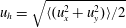 $u_{h}=\sqrt{\langle (u_{x}^{2}+u_{y}^{2})\rangle /2}$
so that
 $u_{h}^{2}$
is the total horizontal kinetic energy and
 $\langle u_{z}^{2}\rangle /2$
is the vertical kinetic energy. The potential energy in our runs is given by
 $E_{p}=\langle b^{2}\rangle /2N^{2}$
.

Visualizations of the buoyancy field in vertical slices corresponding to the central
 $x$
–
 $z$
plane for run R26F0.1 at three different times: (a)
 $t=4.4{\it\tau}_{0}$
(close to the peak in dissipation), (b)
 $t=10{\it\tau}_{0}$
, (c)
 $t=23{\it\tau}_{0}$
. Negative buoyancy goes from dark blue to light blue with a transition in the greys to positive buoyancy going from orange to yellow.

Horizontal slices of the buoyancy field (central
 $x$
–
 $y$
plane) for run R26F0.1 at three different times: (a)
 $t=4.4{\it\tau}_{0}$
, (b)
 $t=10{\it\tau}_{0}$
, (c)
 $t=23{\it\tau}_{0}$
.

Visualizations of
 $b$
in a vertical slice (central
 $x$
–
 $z$
plane) at
 $t=23{\it\tau}_{0}$
for four DNS runs considered: (a) R1.8kF1.8, (b) R330F0.6, (c) R80F0.2, (d) R26F0.1.

The effect of the stratification on the turbulence structure is apparent if we turn to visualizations of vertical and horizontal slices through the parallelepiped-shaped domains (see figures 3 and 4). At the peak in dissipation the buoyancy field is highly turbulent and approximately isotropic (see figure 3
a), but as time progresses and the turbulence dies down,
 $Fr_{h}$
drops and we see the emergence of flattened structures from
 $t=10{\it\tau}_{0}$
onward, while the flow visualized in the horizontal slice in figure 4(b) remains approximately isotropic. At a late time,
 $t=23{\it\tau}_{0}$
, we have reached
 $\mathscr{R}=O(1)$
, and in addition to the continued layering of the turbulence we have clearly a transition to a more viscously dominated flow, with diffuse structures and reduced
 $b$
-gradients (see figures 3
c and 4
c).
Moving on to a comparison of the four low-resolution runs initialized with different Froude numbers at the same non-dimensional time, we see from figure 5 that the layering is more apparent as
 $Fr_{h,ss}$
is lowered (the instantaneous
 $Fr_{h}$
in the four images is decreasing from figure 5(a) to (d)). In addition, we have the interesting feature that the high-
 $Fr_{h,ss}$
runs (R1.8kF1.8 and R330F0.6) still appear vigorously turbulent at this stage, while the low-
 $Fr_{h,ss}$
cases (R80F0.2 and R26F0.1) appear to be in a viscous regime. This observation can be explained if we consider the value of
 $\mathscr{R}$
at this time for the different runs:
 $\mathscr{R}=8.9$
for case R1.8kF1.8,
 $\mathscr{R}=6.3$
for case R330F0.6,
 $\mathscr{R}=3.1$
for case R80F0.2 and
 $\mathscr{R}=1.6$
for case R26F0.1. Hence runs R1.8kF1.8 and R330F0.6 still marginally satisfy
 $\mathscr{R}\gg 1$
at this time and still constitute strongly stratified turbulence, while runs R80F0.2 and R26F0.1 have
 $\mathscr{R}\sim 1$
and they are in a transition phase between the highly turbulent and the viscous regimes of stratified turbulence.
Having obtained a visual appreciation of the stratified turbulence under investigation, we now characterize it quantitatively, looking in particular at the energy dissipation rate, at correlation length scales and at energy spectra.
4.2. Vertical Froude number
One of the main results of our scaling analysis in § 2 is the recovery of the vertical scale relation
 $\ell _{v}\sim u_{h}/N$
as found in the original scaling analysis of the momentum equation by Billant & Chomaz (Reference Billant and Chomaz2001). Of course, this result holds only for high buoyancy Reynolds numbers, or for high values of the parameter
 $\mathscr{R}=ReFr_{h}^{2}$
. However, our runs were intentionally stopped when
 $\mathscr{R}$
falls to order unity, allowing us to check whether
 $\ell _{v}$
scales as the buoyancy scale. When
 $\mathscr{R}=O(1)$
we expect there to be a transition from the scaling
 $\ell _{v}\sim u_{h}/N$
to a viscous scaling. This means that, if we plot
 $Fr_{v}$
as a function of time, we expect it to reach a constant value while
 $\mathscr{R}\gg 1$
. Considering our visualizations in figure 5, the stratified turbulence in our DNS runs appears to change character and be less vigorous at values of
 $\mathscr{R}<6.3$
. We therefore substitute the condition
 $\mathscr{R}>7$
for the more stringent (but not quantifiable) condition
 $\mathscr{R}\gg 1$
, and plot the vertical Froude number as a function of time only for times at which this condition is met. This is done in figure 6 and it is clear that
 $Fr_{v}=\text{const}$
for all runs and the asymptotic value is similar in all cases, at
 $Fr_{v}=0.34{-}0.37$
. We also show the full evolution of
 $Fr_{v}$
(inset panel in figure 6); this shows a slow variation of
 $Fr_{v}$
at late times (especially true for the low-
 $Fr_{0}$
case F0.16) as the stratified turbulence is more affected by vertical viscous diffusion. This is accordance with a transition at
 $\mathscr{R}=O(1)$
between strongly stratified turbulence and a viscously dominated regime.
Evolution of vertical Froude number at times for which
 $\mathscr{R}>7$
for DNS runs. Full
 $Fr_{v}$
evolution is given in the inset.

(a) Total energy dissipation
 ${\it\epsilon}={\it\epsilon}_{k}+{\it\epsilon}_{p}$
normalized by
 $u_{h}^{3}/\ell _{h}$
as a function of time for four runs at different initial
 $Fr$
. The vertical black segment indicates, for each run, the bound between times at which
 $\mathscr{R}>7$
and later times at which
 $\mathscr{R}<7$
.(b) The viscous dissipation and diffusive dissipation normalized analogously for run R49F0.1 with the same bound indicated on the plot.

All in all, the simulations provide convincing evidence that, after an initial transition from random-phase velocity fields to fully developed stratified turbulence, the vertical Froude number is of order one. This is one of the central claims of the strongly stratified turbulence theory and, to our knowledge, it had not been verified in the context of freely decaying simulations.
4.3. Dissipation scaling
It has been suggested by numerous authors that in stratified turbulence both the viscous dissipation
 ${\it\epsilon}_{k}$
and the diffusive dissipation
 ${\it\epsilon}_{p}=(\mathscr{D}/N^{2})(\partial b/\partial x_{i})(\partial b/\partial x_{i})$
scale with horizontal length and velocity scales:
 $$\begin{eqnarray}{\it\epsilon}_{k}=A_{k}\frac{u_{h}^{3}}{\ell _{h}},\quad A_{k}=\text{const};\quad {\it\epsilon}_{p}=A_{p}\frac{u_{h}^{3}}{\ell _{h}},\quad A_{p}=\text{const}.\end{eqnarray}$$
Both constants
 $A_{k}$
and
 $A_{p}$
are expected to be finite and of order one.
In figure 7(a) we show the total energy dissipation rate
 ${\it\epsilon}={\it\epsilon}_{k}+{\it\epsilon}_{p}$
averaged throughout the simulation domain and normalized by
 $u_{h}^{3}/\ell _{h}$
as a function of time for the four runs at the lower resolution. According to the relations (4.1) the quantity
 ${\it\epsilon}\ell _{h}/u_{h}^{3}$
should reach a constant value of order one. We see that this is indeed the case at late times; however, both
 $\mathscr{R}$
and the buoyancy Reynolds number are close to 1 at these times and therefore we expect viscosity to be playing a role here. To clarify further that our four lower resolution simulations are not in the strongly stratified turbulence regime when the curves flatten out, we apply the same bound used in the previous section to test
 $Fr_{v}\sim 1$
. The portions of the four curves presenting a close-to-constant non-dimensional dissipation are all clearly beyond the bound
 $\mathscr{R}=7$
(which corresponds to a buoyancy Reynolds number
 $Re_{b}\approx 2$
).
To understand this apparently contradictory result, we consider the opposite limit to the one treated in the above scaling analysis in § 2, namely the limit of strong viscous dissipation
 $\mathscr{R}\ll 1$
. In this limit, experiments on stratified turbulence (Fincham et al.
Reference Fincham, Maxworthy and Spedding1996) show that vertical diffusion dominates the viscous dissipation and that the flow is still highly anisotropic and composed of pancake structures with
 $\ell _{v}\ll \ell _{h}$
. Given that this flow regime is dominated by the action of viscosity in the vertical direction, we take the vertical length scale to obey a viscous diffusion process
 $\ell _{v}\sim \sqrt{{\it\nu}t}$
, similarly to Godoy-Diana et al. (Reference Godoy-Diana, Chomaz and Billant2004). We also make the assumption that the total dissipation is well described by
 ${\it\epsilon}\sim u_{h}^{3}/\ell _{h}$
, which is what has to be later verified in the scalings. Hence the sum of kinetic and potential energy obeys the evolution equation
 $\text{d}E_{tot}/\text{d}t=-Au_{h}^{3}/\ell _{h}$
. Now, invoking equipartition,
 $E_{k}\sim E_{p}$
, with
 $E_{k}\sim u_{h}^{2}$
and
 $E_{p}\sim b^{2}/N^{2}$
, we arrive at the evolution equation for the horizontal kinetic energy
 $$\begin{eqnarray}\frac{\text{d}u_{h}^{2}}{\text{d}t}=-A_{k}\frac{u_{h}^{3}}{\ell _{h}},\quad u_{h}^{2}\sim t^{-n},\end{eqnarray}$$
where the power-law behaviour is expected as the flow is still turbulent, despite being in the viscous regime. Hence we have
 $$\begin{eqnarray}-n\frac{u_{h}^{2}}{t}=-A_{k}\frac{u_{h}^{3}}{\ell _{h}}\end{eqnarray}$$
from which
 $u_{h}/\ell _{h}=n/(A_{k}t)$
, giving a time scale for this turbulent flow as
 $t=n\ell _{h}/(A_{k}u_{h})\sim \ell _{h}/u_{h}$
(the usual eddy turnover time). Substituting this into our diffusion length
 $\ell _{v}$
we have
 $\ell _{v}\sim \sqrt{{\it\nu}\ell _{h}/u_{h}}=\ell _{h}/\sqrt{Re}$
, a scaling for
 $\ell _{v}$
first proposed by Godoy-Diana et al. (Reference Godoy-Diana, Chomaz and Billant2004) to describe the viscous regime of stratified turbulence. The final step is then to let
 ${\it\epsilon}_{k}\approx {\it\nu}(\partial \boldsymbol{u}_{h}/\partial z)^{2}\sim {\it\nu}u_{h}^{2}/\ell _{v}^{2}\sim u_{h}^{3}/\ell _{h}$
and we have recovered the dissipation scaling for the viscous dissipation. Considering that we are interested in the case
 $Pr={\it\nu}/\mathscr{D}=1$
, which is the case in the DNS runs, the same analysis clearly also leads to
 ${\it\epsilon}_{p}\sim u_{h}^{3}/\ell _{h}$
and therefore the total dissipation
 ${\it\epsilon}$
presents the same scaling. In conclusion we can say with some confidence that this rederivation and figure 7(a) further strengthen the scaling proposed for the viscous regime (see Godoy-Diana et al.
Reference Godoy-Diana, Chomaz and Billant2004; Brethouwer et al.
Reference Brethouwer, Billant, Lindborg and Chomaz2007).
We now consider the high-resolution run R49F0.1. In figure 7(b) the full evolution of this run is presented. It is relatively clear that after an initial transient associated with the stratified turbulence becoming fully developed, the curve flattens out at around
 $t/{\it\tau}_{0}=11.5$
. Again, the boundary demarcating the region in which
 $\mathscr{R}>7$
from the later times at which
 $\mathscr{R}<7$
is given, and it occurs close to the end of the simulation. There is a period of about
 $3{\it\tau}_{0}$
ahead of this boundary during which both
 ${\it\epsilon}_{k}$
and
 ${\it\epsilon}_{p}$
scale with horizontal quantities alone and, when normalized, reach a constant plateau. Despite the fact that the dissipation scaling is presented earlier than the low-resolution runs, at this time we are already in the transition between the strongly stratified regime and the viscous regime. At
 $t/{\it\tau}_{0}=11.5$
,
 $\mathscr{R}=10$
but the buoyancy Reynolds number
 $Re_{b}=2.1$
, as can be seen in figure 8 showing the concurrent evolution of
 $\mathscr{R}$
and
 $Re_{b}$
for runs R80F0.2 and R49F0.1. This value of
 $Re_{b}$
is too low, as can be seen more clearly when calculating the ratio of dissipation due to vertical gradients of horizontal velocity to the total dissipation,
 ${\it\epsilon}_{k,hv}/{\it\epsilon}_{k}=0.69$
at this time. The turbulent motion is starting to be dominated by vertical shear and we are approaching the viscous regime. So we have been unable to verify the dissipation scaling in the strongly stratified regime. Our partial result does, however, support the claim that the dissipation scaling
 ${\it\epsilon}\sim u_{h}^{3}/\ell _{h}$
is a robust result, holding across the various regimes of stratified turbulence.
Comparison of
 $\mathscr{R}$
and buoyancy Reynolds number for two low-
 $Fr_{h,ss}$
runs, R80F0.2 and R49F0.1. The full evolution in time is shown.

4.4. Horizontal spectra of horizontal kinetic energy
According to Lindborg (Reference Lindborg2006) the horizontal spectrum of horizontal kinetic energy (which is very similar to the spectrum of full kinetic energy, given that the vertical component of velocity is small) should scale as
 $E_{h}(k_{h})\sim {\it\epsilon}_{k}^{2/3}\,k_{h}^{-5/3}$
for strongly stratified turbulence. Let us now see if this is the case for our decaying runs. Figure 9 shows one-dimensional horizontal spectra of horizontal kinetic energy compensated by multiplication by
 ${\it\epsilon}_{k}^{-2/3}k_{h}^{5/3}$
for the four DNS runs. These compensated spectra should present a plateau at a constant value of
 $\tilde{E}_{h}(k_{h})={\it\epsilon}_{k}^{-2/3}k_{h}^{5/3}E_{h}(k_{h})$
over the stratified inertial range if the Lindborg scaling applies. We have chosen to plot the spectra using a linear axis for the
 $y$
-axis as often log–log plots show apparent plateaus where there is still significant variation in the compensated spectra. We can see that the compensated spectra present about half a decade of constancy for runs F1.3, F0.6 and F0.3, starting from a wavenumber
 $k_{h}\approx 10$
. We have chosen the time instants in figure 9 as they present the clearest stratified inertial range and these times correspond to
 $\mathscr{R}\approx 15$
for the three runs with a clear plateau. This is in line with previous knowledge (Bartello & Tobias Reference Bartello and Tobias2013) that
 $Re\,(\ell _{v}/\ell _{h})^{2}=10$
appears to be the lower bound for the strongly stratified horizontal spectra to be observed. In our DNS simulations this condition actually would translate to
 $Re\,Fr_{h}^{2}/Fr_{v}^{2}\approx 8Re\,Fr_{h}^{2}=8\mathscr{R}>10$
or
 $\mathscr{R}>1.3$
using the value
 $Fr_{v}=0.35$
reached by all our runs. We find in our runs that
 $\mathscr{R}\approx 15$
is needed for the stratified inertial range to be observed. The extent of the stratified inertial range should be from the horizontal integral scale to the Ozmidov scale, and this range is determined solely by the Froude number since
 $k_{oz}/k_{\ell _{h}}\sim Fr_{h}^{-3/2}$
(Lindborg Reference Lindborg2006). Hence the lower the Froude number the more wavenumbers the inertial range covers, and this is consistent with our results with run F0.3 presenting the longest inertial range.
Compensated horizontal spectra of horizontal kinetic energy,
 $\tilde{E}_{h}(k_{h})={\it\epsilon}_{k}^{-2/3}k_{h}^{5/3}E_{h}(k_{h})$
. (a) Run R18.kF1.8 at
 $t=20.4{\it\tau}_{0}$
(
 $\mathscr{R}=14.6,\;Fr_{h}=0.16$
), (b) run R330F0.6 at
 $t=12.3{\it\tau}_{0}$
(
 $\mathscr{R}=15.9,\;Fr_{h}=0.12$
), (c) run R80F0.2 at
 $t=8.8{\it\tau}_{0}$
(
 $\mathscr{R}=15.6,\;Fr_{h}=0.096$
), (d) run R26F0.1 at
 $t=5.4{\it\tau}_{0}$
(
 $\mathscr{R}=20,\;Fr_{h}=0.11$
). (e) Run R49F0.1 at
 $t=5.6{\it\tau}_{0}$
(
 $\mathscr{R}=29.7,\;Fr_{h}=0.11$
).

There is a limit, however, to how low we can push the Froude numbers in a decaying context, as exemplified by run R26F0.1 where no stratified inertial range is visible. We interpret this as the effect of the vertical dissipation of large-scale horizontal motions, which becomes important at
 $\mathscr{R}=O(10)$
. Clearly, since
 $\mathscr{R}=Re\,Fr_{h}^{2}$
, this occurs at earlier times for runs that start from low
 $Fr_{ss}$
. Now, the stratified cascade with its inertial range inevitably sets in after the dissipation peak and formation of smallest scales. As a result it appears that, for the case R26F0.1, there is not enough time for the spectrum to become fully developed before vertical diffusion dominates. To add some numerical evidence to this argument, all runs present a peak in dissipation at
 $t=4.4{\it\tau}_{0}$
and we have
 $\mathscr{R}=15$
at a later time highly dependent on
 $Fr_{h,ss}$
. For the case R26F0.1 this time is
 $t=6.6{\it\tau}_{0}$
(for the other runs the times are given approximately in figure 9), and hence two initial eddy turnover times are not sufficient for the stratified cascade to fully develop. On the other hand run R80F0.2 has about 4.5 turnover times before diffusion starts becoming important so that an inertial range can be established.
The bottom plot in figure 9 corresponds to run R49F0.1 at an early time. At this instant, there is no plateau observable on the horizontal spectrum of horizontal kinetic energy, but rather a dip at
 $k_{h}\approx 20$
and a bump at
 $k_{h}\approx 80$
, similarly to what was observed by Augier et al. (Reference Augier, Billant and Chomaz2015).
Horizontal spectra of horizontal kinetic energy compensated such that
 $\tilde{E}_{h}(k_{h})={\it\epsilon}_{k}^{-2/3}k_{h}^{5/3}E_{h}(k_{h})$
for (a) R330F0.6 from
 $t=11{\it\tau}_{0}$
up to
 $t=13.6{\it\tau}_{0}$
(horizontal line corresponds to
 $\tilde{E}_{h}=0.44$
), (b) R80F0.2 from
 $t=7.4{\it\tau}_{0}$
up to
 $t=9.6{\it\tau}_{0}$
(horizontal line corresponds to
 $\tilde{E}_{h}=0.43$
).

The compensated spectra in figure 9 are for a given time instant. It is interesting to observe the evolution of the spectra in time to check whether the scaling with the kinetic energy dissipation is correct. Results for the one-dimensional horizontal spectra of horizontal kinetic energy over a range of times are presented in figure 10 for cases R330F0.6 and R80F0.2. It is clear that the curves collapse well over two to three integral time scales, showing that the dependence on the kinetic energy dissipation is met in our simulations. Moreover, the constant describing the compensated horizontal spectra is
 $C_{1}=0.44\pm 0.02$
for the four runs excluding run R26F0.1. For times beyond the ones considered in figure 10 the spectra are viscously dominated without much of an inertial range, highlighting that the buoyancy Reynolds number is low at late times.
It is important to note that
 $k_{h}^{-5/3}$
horizontal spectra are presented well before the dissipation scaling
 ${\it\epsilon}\sim u_{h}^{3}/\ell _{h}$
is shown, meaning that the result for the spectra is applicable to the regime of strongly stratified turbulence. For instance, the high-resolution run has
 ${\it\epsilon}_{k,hv}/{\it\epsilon}_{k}=0.419$
at the time at which the spectra are shown, which is not too far from the isotropic value of
 ${\it\epsilon}_{k,hv}/{\it\epsilon}_{k}=4/15=0.267$
. The
 $-5/3$
form of the horizontal kinetic energy spectra is a statement that the dissipation scaling holds on a scale-by-scale basis, or
 $v_{h}^{3}/s_{h}\sim {\it\epsilon}_{k}$
where
 $v_{h}$
and
 $s_{h}$
are local scales in the cascade. It is therefore surprising that this scaling holds in the inertial range in our DNS runs but, at the same times, not at the integral scales, which are feeding the downscale cascade of energy in the horizontal. At high enough
 $\mathscr{R}$
and buoyancy Reynolds number it is expected that both results will be recovered, but in our simulations the horizontal-transfer-to-dissipation balance is found scale-by-scale but not in a volume-averaged sense.
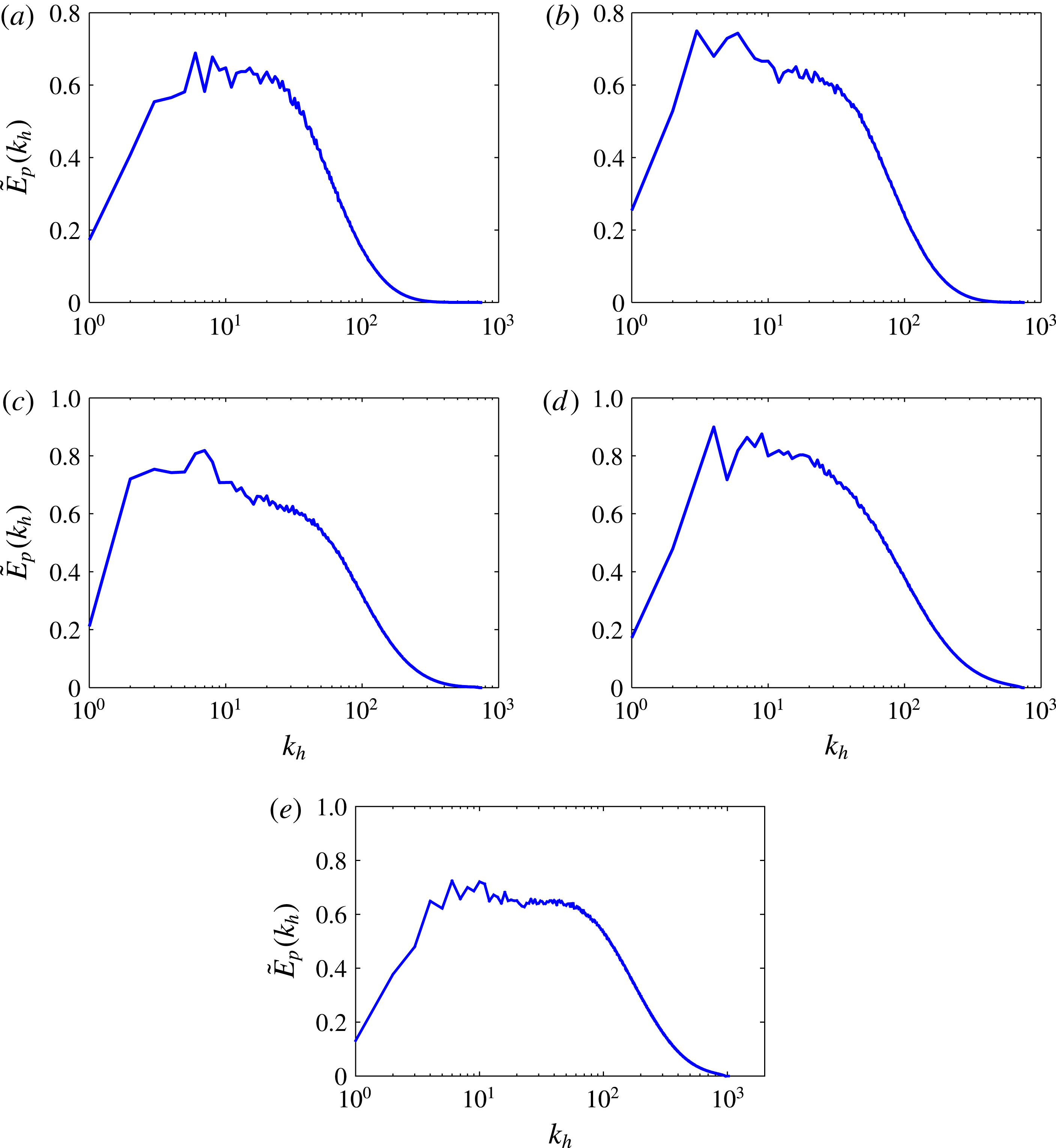
Compensated horizontal spectra of potential energy,
 $\tilde{E}_{p}(k_{h})={\it\epsilon}_{p}^{-1}{\it\epsilon}_{k}^{1/3}k_{h}^{5/3}E_{p}(k_{h})$
. The runs and corresponding times are the same as those given in figure 9.
4.5. Horizontal spectra of potential energy
The horizontal spectra of potential energy predict that
 $E_{p}(k_{h})\sim {\it\epsilon}_{p}{\it\epsilon}_{k}^{-1/3}k_{h}^{-5/3}$
, which is found from cascade arguments (analogous to those that lead to the form for the horizontal spectrum of horizontal kinetic energy) and on insisting that the time scale of the buoyancy fluctuations is the same as the convective time scale. It follows from this that the form of the horizontal spectrum is a Corrsin–Obukhov spectrum, which governs passive scalar advection. Figure 11 shows five compensated horizontal spectra of potential energy, one for every run at the same times as for the horizontal kinetic energy spectra in figure 9. Except for the high-resolution run R49F0.1 presenting a clear inertial range behaviour, the results are less convincing than the kinetic energy spectra. Nonetheless the spectra present a limited inertial range as shown more clearly by the time evolution of the potential energy spectra for runs F0.6 and F0.3 in figure 12. The constant appears to be
 $C_{2}=0.61\pm 0.03$
across the runs, except for case R26F0.1 where, as for the kinetic energy spectra, there is no clear plateau.
Compensated horizontal 1-D spectra of potential energy with
 $\tilde{E}_{p}(k_{h})={\it\epsilon}_{p}^{-1}{\it\epsilon}_{k}^{1/3}k_{h}^{5/3}E_{p}(k_{h})$
for (a) F0.6 from
 $t=11{\it\tau}_{0}$
up to
 $t=13.1{\it\tau}_{0}$
(horizontal line corresponds to
 $\tilde{E}_{p}=0.61$
), (b) F0.3 from
 $t=7.4{\it\tau}_{0}$
up to
 $t=8.8{\it\tau}_{0}$
(horizontal line corresponds to
 $\tilde{E}_{p}=0.62$
).

4.6. Horizontal energy flux spectra
We have calculated the horizontal energy flux spectra
 ${\it\Pi}_{k}(k_{h})$
and
 ${\it\Pi}_{p}(k_{h})$
by summing the transfer spectra over cylinders of radius
 $k_{h}$
in Fourier space; here
 $k_{h}$
is a two-dimensional wavenumber,
 $k_{h}=\sqrt{k_{x}^{2}+k_{y}^{2}}$
. For more details on the definition of kinetic energy and potential energy transfer spectra the reader is referred to Augier, Chomaz & Billant (Reference Augier, Chomaz and Billant2012). The horizontal energy flux spectra highlight the energy transfers in the horizontal direction at a certain wavenumber
 $k_{h}$
. If
 ${\it\Pi}_{k}(k_{h})>0$
then there is downscale transfer of kinetic energy to higher wavenumbers than
 $k_{h}$
, and if
 ${\it\Pi}_{k}(k_{h})<0$
there is an upscale transfer at this wavenumber. Moreover, a region of constant
 ${\it\Pi}_{k}$
or
 ${\it\Pi}_{p}$
defines an inertial range (see Lindborg Reference Lindborg2006). In figure 13 we show
 ${\it\Pi}_{k}$
and
 ${\it\Pi}_{p}$
together with the corresponding 2-D horizontal spectra for runs R80F0.2 and R49F0.1. The times at which the energy flux spectra are shown are towards the end of the period over which the 1-D spectra present a collapse over time (see figure 10). The energy spectra are compensated to show a
 $k_{h}^{-5/3}$
-range, which is very limited in run R80F0.2 and slightly more pronounced in the high-resolution run R49F0.1. In all cases the energy flux spectra are constant over a narrow range, which correlates well with the
 $k_{h}^{-5/3}$
-region in the 2-D spectra (except for
 ${\it\Pi}_{k}$
in run R80F0.2, which is flat starting from wavenumbers
 $k_{h}<10$
, where there is clearly no
 $k_{h}^{-5/3}$
-region). In both runs, the region
 ${\it\Pi}_{p}=\text{const.}$
extends to higher wavenumbers than the region
 ${\it\Pi}_{k}=\text{const}$
. The ranges are narrow due to the limited dynamic range in the runs, but the fact that
 ${\it\Pi}_{k}$
and
 ${\it\Pi}_{p}$
present a region of constancy provides confirmation that we indeed have an inertial range in the horizontal direction. The kinetic and potential energy fluxes are negative at small wavenumbers, showing that there is a small upscale transfer at large scales. However, in both the runs under consideration, the transfer of kinetic energy to the shear modes
 $k_{h}=0$
is negligible at the times shown, and it is actually downscale for run R80F0.2 from this mode. At other times, there is a transfer of kinetic energy towards the
 $k_{h}=0$
mode but this mode never dominated the dynamics in our simulations.
As is apparent from figure 13 we have
 ${\it\Pi}_{k}<{\it\epsilon}_{k}$
and
 ${\it\Pi}_{p}<{\it\epsilon}_{p}$
in the inertial range. If we form total transfers
 ${\it\Pi}={\it\Pi}_{k}+{\it\Pi}_{p}$
then the ratio of the total transfer to the total dissipation is
 ${\it\Pi}/{\it\epsilon}\approx 0.53$
in the inertial range for both runs under consideration. Hence only about half of the dissipation rate can be attributed to downscale transfer of energy in the horizontal in our decaying stratified turbulence. This means that the remaining half of the dissipation rate must be accounted for by energy transfers in the vertical direction or by dissipation acting at scales of the order
 $k_{h}\approx 30$
or lower, presumably due to vertical shear at these horizontal scales. The cascade of energy in the horizontal has therefore been confirmed in our DNS of stratified turbulence but perhaps it should be put into perspective that it accounts for only roughly half of the total energy dissipation in the flow. Further simulations with a greater dynamic range are needed to confirm this statement.
Energy flux spectrum in the horizontal direction together with the corresponding horizontal 2-D spectrum (compensated): (a) horizontal kinetic energy spectrum
 $\tilde{E}_{h}(k_{h})={\it\epsilon}^{-2/3}k_{h}^{5/3}E_{h}(k_{h})$
and kinetic energy flux spectrum for run R80F0.2, (b) potential energy spectrum
 $\tilde{E}_{p}={\it\epsilon}_{p}^{-1}{\it\epsilon}_{k}^{1/3}k_{h}^{5/3}E_{p}(k_{h})$
and potential energy flux spectrum for run R80F0.2 (both (a) and (b) are at
 $t/{\it\tau}_{0}=9.3$
), (c) horizontal kinetic energy spectrum and horizontal kinetic energy flux spectrum for run R49F0.1, (d) potential energy spectrum and potential energy flux spectrum for run R49F0.1 (both (c) and (d) are at
 $t/{\it\tau}_{0}=7.5$
). The horizontal wavenumber is incremented by 0.5 to show the transfers to the shear modes with
 $k_{h}=0$
.

4.7. Vertical energy spectra
Vertical spectra of horizontal kinetic and potential energy are predicted to scale as
 $E_{h}(k_{v})\sim E_{p}(k_{v})\sim N^{2}k_{v}^{-3}$
according to the strongly stratified turbulence theory. This particular form for
 $E_{h}(k_{v})$
means that the vertical Froude number is of order unity on a scale-by-scale basis. It is important to test whether the vertical spectra in our decaying runs obey this scaling or not. In figure 14(a), vertical spectra of horizontal kinetic energy for all four cases at specific times are presented, the spectra having been compensated so that a horizontal plateau would show accordance with the scaling above. There is no evidence of such a plateau in any of the DNS runs, the spectra being considerably shallower than
 $k_{v}^{-3}$
before the rapid viscous decay at high wavenumbers. Similar vertical spectra were found by Bartello & Tobias in their decaying simulations (S. M. Tobias 2014, personal communication).
It should be pointed out that the range of vertical wavenumbers at which the
 $k_{v}^{-3}$
-spectrum is predicted is narrow, the scales ranging from the buoyancy scale
 $u_{h}/N$
to the Ozmidov scale
 $\ell _{oz}=\sqrt{{\it\epsilon}_{k}/N^{3}}$
, which scales like
 $Fr_{h}^{-1/2}$
(see Lindborg Reference Lindborg2006). Given the moderately low Froude number in our runs, which is
 $Fr_{h}=O(0.1)$
during the time when
 $\mathscr{R}=O(10)$
, the results for vertical spectra are not so surprising. Limited support has been provided to date for such steep vertical spectra: Augier et al. (Reference Augier, Chomaz and Billant2012) have found
 $k_{v}^{-3}$
-vertical spectra in their simulations of transient evolution of the zigzag instability while Almalkie & de Bruyn Kops (Reference Almalkie and de Bruyn Kops2012) have found this scaling in only one of their high-resolution forced runs of stratified turbulence.
The vertical spectra in our DNS runs at intermediate to late times are actually rather similar to their horizontal equivalents, as shown in figure 14(b) for both kinetic and potential energy. The vertical and horizontal spectra present closely matching trends at varying wavenumber, meaning that the vertical spectra are closer to
 $k_{v}^{-5/3}$
than
 $k_{v}^{-3}$
over the stratified inertial range. Beyond a transition wavenumber that corresponds to the Ozmidov scale
 $\ell _{oz}$
it is expected that there is a return to an isotropic Kolmogorov spectrum of the form
 $E_{h}(k_{v})\sim {\it\epsilon}_{k}^{2/3}k_{v}^{-5/3}$
(see Brethouwer et al.
Reference Brethouwer, Billant, Lindborg and Chomaz2007; Augier et al.
Reference Augier, Chomaz and Billant2012). Our shallow vertical spectra may be the result of an early transition to isotropic conditions due to the moderately low
 $Fr_{h}$
. We will discuss this point further in the discussion that follows in § 5.
(a) Compensated vertical spectra of horizontal kinetic energy,
 $\tilde{E}_{h}(k_{v})=N^{-2}k_{v}^{3}E_{h}(k_{v})$
. (b) Horizontal and vertical 1-D spectra of horizontal kinetic energy (main plot) and potential energy (inset) for the case R1.8kF1.8 at
 $t=27.2{\it\tau}_{0}$
.

5. Discussion
The fact that the vertical spectra do not present an
 $N^{2}k_{v}^{-3}$
-dependency has an important implication: the vertical Froude number is not of order unity on a scale-by-scale basis in our simulations. We will now see that this is actually not so surprising if we consider that our scaling argument from which we found
 $Fr_{v}\sim 1$
implies that
 $Fr_{h}\ll 1$
. Let us consider scale-by-scale Froude numbers
 $Fr_{s_{h}}=v_{h}/Ns_{h}$
and
 $Fr_{s_{v}}=v_{h}/Ns_{v}$
, where
 $v_{h}$
,
 $s_{h}={\rm\pi}/k_{h}$
and
 $s_{v}={\rm\pi}/k_{v}$
are local scales in the cascade. The reason for using a factor of
 ${\rm\pi}$
and not
 $2{\rm\pi}$
when relating a scale to its corresponding wavenumber is that
 $s_{h}$
and
 $s_{v}$
are scales and not wavelengths, i.e. a region of correlated positive buoyancy such as a yellow structure in figure 3 presents scales
 $s_{h}$
and
 $s_{v}$
while if we consider also an adjacent blue structure we will have a wavelength. We found some evidence from our horizontal spectra that at intermediate scales in the inertial range we should have
 ${\it\epsilon}\sim v_{h}^{3}/s_{h}$
. This leads to
 $$\begin{eqnarray}Fr_{s_{h}}=\frac{v_{h}}{Ns_{h}}\sim \frac{({\it\epsilon}s_{h})^{1/3}}{Ns_{h}}=\frac{{\it\epsilon}^{1/3}k_{h}^{2/3}}{{\rm\pi}^{2/3}N}\end{eqnarray}$$
so it is clear that
 $Fr_{s_{h}}$
steadily grows from its integral scale value
 $Fr_{h}$
as we move to smaller scales. Run F0.3 presents the clearest inertial range of
 $E_{h}(k_{h})$
– see figure 9 – but on substituting the values of dissipation at this time in (5.1), we see that
 $Fr_{s_{h}}>Fr_{v}$
for
 $k_{h}>80$
. This value compares well with the wavenumber at the end of the stratified inertial range, estimated to be
 $k_{h}=50$
, as can be seen in figures 9 and 10. However, this value of
 $k_{h}$
is only about 10 vertical wavenumbers after the peak in
 $E_{h}(k_{v})$
so it appears that the condition
 $Fr_{s_{h}}\ll 1$
is not well satisfied for most of the vertical scales and
 $Fr_{s_{v}}$
can therefore not be of order unity for these scales. The typical argument reads that the horizontal Froude number becomes unity at the Ozmidov scale with
 $k_{oz}={\rm\pi}\sqrt{N^{3}/{\it\epsilon}_{k}}\approx 470$
for run F0.3 at
 $t=8.8{\it\tau}_{0}$
(the time of figure 9). But, by using the value of
 $Fr_{v}$
from our simulations, the estimate for the transition wavenumber is greatly reduced (the use of the total dissipation also reduces this value, but by a much smaller amount), making it practically impossible to observe a vertical inertial range as predicted by the strongly stratified turbulence theory.
In the future, greater computer capabilities will allow
 $Fr_{h}$
to be pushed much lower, while keeping
 $\mathscr{R}>O(10)$
, thus allowing
 $Fr_{s_{h}}$
to be small over a large range of scales. The scaling analysis of § 2 should therefore be valid over these scales, for which
 $Fr_{s_{v}}\sim 1$
as a result. It follows that the level of anisotropy decreases as we go down the cascade:
 $$\begin{eqnarray}\frac{v_{z}}{v_{h}}\sim \frac{s_{v}}{s_{h}}=\frac{Fr_{s_{h}}}{Fr_{s_{v}}}\sim Fr_{s_{h}}\sim \frac{{\it\epsilon}^{1/3}k_{h}^{2/3}}{N},\end{eqnarray}$$
where
 $v_{z}$
is a local vertical velocity scale and we have used continuity in the first step. Therefore the distribution of vertical kinetic energy across horizontal scales is given by
 $$\begin{eqnarray}v_{z}^{2}\sim \left(\frac{{\it\epsilon}^{1/3}k_{h}^{2/3}}{N}\right)^{2}\left(\frac{{\it\epsilon}}{k_{h}}\right)^{2/3}\sim \frac{{\it\epsilon}^{4/3}k_{h}^{2/3}}{N^{2}},\end{eqnarray}$$
which grows as we move to smaller and smaller scales up to a transition wavenumber that is of the order of
 $k_{oz}$
. This means that, as discussed previously by Davidson (Reference Davidson2013) and Riley & Lindborg (Reference Riley, Lindborg, Davidson, Kaneda and Sreenivasan2013), the vertical velocity fluctuations peak at the Ozmidov scale,
 $\ell _{oz}$
, rather than at the integral scale
 $\ell _{h}$
. From (5.3) we therefore have
 $\langle u_{z}^{2}\rangle \sim v_{z}^{2}(k_{h}=k_{oz})\sim {\it\epsilon}/N$
, from which the following result is obtained:
 $$\begin{eqnarray}\frac{\langle u_{z}^{2}\rangle }{u_{h}^{2}}\sim \frac{{\it\epsilon}/N}{u_{h}^{2}}\sim \frac{u_{h}}{N\ell _{h}}=Fr_{h}\end{eqnarray}$$
rather than
 $\langle u_{z}^{2}\rangle =Fr_{h}^{2}\;u_{h}^{2}$
, the naive deduction obtained by applying continuity without realizing that vertical velocity is a small-scale quantity in stratified turbulence.
We have attempted to test equation (5.4) in our simulations. However, large oscillations with frequency equal to twice the Brunt–Väisälä frequency on the
 $\langle u_{z}^{2}\rangle$
-curve appear to cause a mismatch between
 $\langle u_{z}^{2}\rangle /u_{h}^{2}$
and
 $Fr_{h}$
. This can be observed in figure 15. By removing the mode
 $k_{z}=0$
from the vertical 1-D spectra of
 $u_{z}^{2}$
, one isolates the dynamics that is independent of this
 $k_{z}=0$
wavenumber, at which the oscillations are expected according to the IGW dispersion relation. The summation of the 1-D spectra of
 $u_{z}^{2}$
from the first non-zero vertical wavenumber to the largest vertical wavenumber is presented together with the evolution of
 $Fr_{h}$
in time in figure 15. The match of functional forms is good for both low-
 $Fr_{h,ss}$
runs considered: run R80F0.2 and the high-resolution run R49F0.1.
Evolution of the non-dimensionalized vertical velocity variance and the horizontal Froude number in (a) run R80F0.2, (b) run R49F0.1. The solid grey curve (cyan online) corresponding to
 $\langle u_{z}^{2}\rangle |^{k_{z}\neq 0}/u_{h}^{2}$
represents the variance of
 $u_{z}$
(non-dimensionalized by
 $u_{h}^{2}$
), with the removal of the contributions to the variance of the wavenumber
 $k_{z}=0$
. The solid dark curve (red online) corresponds to the horizontal Froude number. The dashed curve (green online) with the large and periodic oscillations is the variance of
 $u_{z}^{2}$
non-dimensionalized by
 $u_{h}^{2}$
considering all vertical wavenumbers.

Another observation that we may add to support this relation is that visualizations of
 $u_{z}$
appear to be isotropic as seen in figure 16, at variance with the other fields,
 $u_{x}$
,
 $u_{y}$
and
 $b$
, which invariably present the characteristic layering of stratified turbulence (see figures 3–5). This is suggestive of
 $u_{z}$
being a smaller scale quantity, as at small scales we have a return to isotropy. It is hoped that further simulations of stratified turbulence at lower
 $Fr_{h}$
will confirm these preliminary findings.
Visualization of the
 $u_{z}$
field in run R80F0.2 at
 $t/{\it\tau}_{0}=10$
, corresponding to
 $Fr_{h}=0.09$
and
 $\mathscr{R}=13.3$
.

6. Conclusions
We have presented results from a scaling analysis and DNS of stratified turbulence starting from a high value of
 $\mathscr{R}$
and a Froude number of order one. The alternative scaling analysis based upon the vorticity equations leads simply and directly to the well-known scaling result for the vertical length scale of the turbulence as
 $\ell _{v}=u_{h}/N$
. In doing so it highlights the importance of horizontal vorticity in stratified turbulence, and in particular of vertical shearing of horizontal velocity at large scales (which can be interpreted physically as pancake vortices sliding one on top of the other). The DNS results are in line with the scaling prediction on the vertical scale at high
 $\mathscr{R}$
and show the first signs of a transition to a viscous scaling at
 $\mathscr{R}=O(1)$
.
A frequent assumption in the literature on stratified turbulence is
 ${\it\epsilon}_{k}\sim u_{h}^{3}/\ell _{h}$
and
 ${\it\epsilon}_{p}\sim u_{h}^{3}/\ell _{h}$
, which can be useful when interpreting the results of forced simulations. The results of our runs have shown its validity, yet only for the transition regime between the strongly stratified turbulence and the viscous regimes. This result does suggest that the dissipation scaling is robust, holding across the regimes of stratified turbulence. The horizontal spectra are largely in line with the Lindborg forms over a limited inertial range. The presence of an inertial range is confirmed by the energy flux spectra
 ${\it\Pi}_{k}$
and
 ${\it\Pi}_{p}$
being approximately constant over a narrow
 $k_{h}$
-range. The
 $k_{h}^{-5/3}$
-spectra are observed from early times so that we are still in a state close to strongly stratified turbulence. The reason why the spectra present
 $k_{h}^{-5/3}$
-ranges at times when the dissipation does not show
 ${\it\epsilon}\sim u_{h}^{3}/\ell _{h}$
is not understood, and is a point that deserves further attention. The constants
 $C_{1}$
and
 $C_{2}$
for the horizontal kinetic and potential energy spectra are different in our runs, while previous results had them as being very close with
 $C_{1}=C_{2}\approx 0.5$
as found by Lindborg (Reference Lindborg2006) and Lindborg & Brethouwer (Reference Lindborg and Brethouwer2007). More importantly, the vertical spectra
 $E_{h}(k_{v})$
and
 $E_{p}(k_{v})$
are very far from
 $k_{v}^{-3}$
and are closer to
 $k_{v}^{-5/3}$
over a range of wavenumbers. This result is thought to be due to the insufficiently low horizontal Froude numbers in the cases under consideration. It is possible that by pushing horizontal Froude numbers down to very low values
 $Fr_{h}=O(10^{-3})$
the form
 $N^{2}k_{v}^{-3}$
for the vertical spectra will be recovered and the scaling
 $Fr_{v}\sim 1$
will be found to hold over a range of scales. The computational requirements for such a run are very high, but they could lead to the resolution of an important open issue in stratified turbulence.
Acknowledgement
The authors would like to thank Professor P. K. Yeung of Georgia Tech for valuable discussions and for providing the pseudo-spectral code used for the simulations.



