“To arrive at some understanding of what is going on is hard enough,” says Abraham Kaplan, “without having also to meet the demand that we anticipate what will happen next” (1964, 351). Despite Kaplan's warning, attempts at forecasting American elections by political scientists have grown in recent years. Foreshadowing election results is not just a casual interest for political scientists. It both sparks interest in the work of our discipline, and serves as a pedagogical tool. We admit that many challenges present themselves when we attempt to predict complicated social phenomena; but if we, instead, limit our research to description and explanation, the danger is that repeated analysis of the same datasets will track patterns again and again that do not exist in the reality outside our samples. One guard against this is to take theories about politics and employ them to predict future events. In this spirit, this paper utilizes well-known patterns of congressional elections to predict those of the 2006 Senate.
Over the last 30 years, forecasting presidential elections has become something of a cottage industry among political scientists. Notable early examples include the work of Sigelman (1979) and Rosenstone (1983). More recently, the October 2004 issue of PS was devoted to forecasting that year's upcoming presidential election. In that issue, PS published seven forecasting models by well-known scholars. The median estimate of these forecasts was fairly close to the actual election outcome: about 2.5% off, in fact (Campbell 2005).Forecasting models published in PS and elsewhere for the 2000 election were less successful at predicting election outcomes, although this failure may be explained as the result of a lack of access to essential data (Bartels and Zaller 2001).
Attempts at forecasting elections for the U.S. House of Representatives have been fairly common, although House elections have not received quite as much attention as presidential elections. An early example of House election forecasting was made by Tufte (1975), who utilized presidential approval and change in per capita income to predict the number of seats that would change hands in an election. Recent examples of models predicting the 2002 midterm House elections were showcased on the American Political Science Association's Elections, Public Opinion and Voting Behavior section web site.1
One of the most notable of these models was published by Lewis-Beck and Tien (reported in Bardwell and Lewis-Beck 2004). Using presidential approval numbers, income growth, and a dummy variable indicating a midterm election year, Lewis-Beck and Tien predicted an eight-seat gain by the Democrats in 2004. The outcome was a Republican gain of six seats. Well-known forecasters have made their predictions for the 2006 elections using similar models (Abramowitz 2006).Fewer forecasting attempts have been made to predict U.S. Senate elections (Bardwell and Lewis-Beck 2004). Senate forecasting models have typically utilized information about the strength of the economy, presidential approval, and seat exposure. An early attempt at explaining Senate elections was made by Hibbing and Alford (1982), although they did not make out-of-sample forecasts. Abramowitz and Segal (1986) made predictions about the outcome of the 1986 election, although their predictions were contingent on the value of presidential approval and the change in real disposable income that occurred after publication of their article. In 2002, to forecast the Senate election that year, Lewis-Beck and Tien updated the 1986 Abramowitz-Segal model. Lewis-Beck and Tien's (2002) prediction turned out to have been five seats off the actual change of seats (Lewis-Beck and Tien's 2002 model is reported in Bardwell and Lewis-Beck 2004). Abramowitz (2006) has also made predictions for the U.S. Senate for the 2006 elections, predicting a 2.2 seat gain for the Democrats.
Political scientists' models contrast with the more district-oriented approach used by other experts in predicting congressional elections. Others typically use district- or state-level information to forecast election results. Sometimes these predictions are aided by district-level polls of varying quality. Examples are the predictions published in Congressional Quarterly for all House and Senate elections.
In contrast, political scientists typically use what we refer to as the aggregate approach to forecasting elections. Scholars using the aggregate approach examine past elections. They compare the number of seats that change party hands to various measures of a national partisan tide. A national partisan tide is represented by such factors as the health of the economy, presidential approval, the quality of candidates running for each party, or stated intentions of the voters (Jacobson 2004; Abramowitz 2002). Scholars using this approach estimate the magnitude of these relationships and take the current values of the independent variables to predict future elections (Abramowitz and Segal 1986; Abramowitz 2002).
The aggregate method and the district-oriented method each has its strengths and its weaknesses, but combining the two methods, as we have done in this paper, takes advantage of the strengths of both.
The strength of the district-level approach is that it recognizes the importance of district-level factors in influencing election outcomes. The weakness is that it may not accurately assess the size of a national partisan tide. The strength of the aggregate approach is that it is better at assessing such a tide. Its weakness is that it does not assess how such a national partisan tide may interact with district-level factors. For example, if there is a large national partisan tide, its impact on how many seats change hands is contingent on the number of “swing districts”—districts won by only a few percentage points. Similarly, the impact of “quality” challengers running for each party is contingent on where such candidates are running. They may be running in very competitive districts, or they may be running in only marginally competitive districts. Combining both approaches by using a panel model, that is, a model that combines many different time series into one pooled dataset, overcomes both of these problems. Both national and district conditions, as well as how those conditions combine to influence election outcomes may be examined.
Another potential problem with using the “aggregate approach” for Senate elections is the staggered nature of senators' terms. Only one of the three classes of senators is up for election in any election year. This makes assessing the impact of national level forces potentially problematic. An aggregate model does not take into account which two-thirds of the states are having Senate elections in the forecast year. Which states' Senate seats are up for election can have a major impact on national election outcomes due to the varied strength of the parties from state to state. Grofman, Brunell, and Koetzle (1998) take this problem into account when using the aggregate approach to explain Senate elections. A simpler solution is to move to the pooled approach utilized here.
A related, although smaller, problem for the aggregate approach is that the number of Senate seats up for election varies slightly from year to year. There are a couple of reasons for this variation. Occasionally, elections for vacant seats from either or both of the two other classes occur. And during every third senatorial election year, 34 states, not 33, hold elections for senator. This may sound trivial, but when the average change in seats held by Democrats in a Senate election since 1960 is 3.32, and the median is 2.5, it is not. A “pooled approach” does not present these problems.
The rest of this article explains this modeling strategy and its predictions, made June 30, 2006, for the 2006 midterm Senate elections.
Methodology
The dependent variable of this analysis is the percent of the two-party vote that goes to Democrats. These data are from Congressional Quarterly's (CQ's) Voting and Elections Collection.2
This database was accessed through the Grinnell College library web site at www.lib.grinnell.edu/db.php, accessed May 2005.
The partisan composition of states is measured in two ways, both following Highton (2000). The first is to average the two-party vote for Democrats from the two most recent Senate elections in the state (Past Senate Vote). The second is to average the results from the two most recent presidential elections in the state, after altering them in the following way: the percent of the Democratic presidential two-party vote in the nation as a whole in a particular election is subtracted from the Democratic share of the two-party vote in each state (Past Presidential Vote). This is done so that national partisan tides favoring a certain party in a presidential election are subtracted from presidential vote returns. (For a full explanation, see Highton [2000]). These variables are also from CQ's Voting and Elections Collection, cited above.
Three attributes of Senate candidates are included in the model: whether candidates are incumbents; the voting record of incumbents; and the prior office-holding experience of non-incumbents. The variable “Incumbent” has a score of “−1” if the Republican candidate is an incumbent, and “1” if the Democratic candidate is an incumbent. Unelected incumbents and past incumbents are given scores of “0.” A vast literature supports the notion that incumbents get a much larger share of the vote than non-incumbents. (See Jacobson [2004] for citations charting this phenomenon.) The coefficient calculated for this variable can be interpreted to mean the increase (assuming a positive coefficient) in the percent of the vote a party's candidate will receive if the candidate is an incumbent, compared to the percent of the vote a candidate who is not an incumbent receives.
The voting records of incumbents are captured by the variable “Roll-Call Conservatism.” This variable is Keith Poole's well known NOMINATE score, which varies from “−1” to “1”, with higher scores representing more conservative voting records.3
These data were obtained at http://voteview.com/dwnomin.htm, accessed June 25, 2006. This variable was added to the model at a reviewer's request.
The previous office holding experience of non-incumbents is measured by a variable labeled “Previous Office Holding.” This indicator, similar to one created by Squire (1989), gives points on the basis of the value of previous offices held for electoral success. State legislators are given scores of “1,” statewide officers (excluding governors) are given scores of “2,” members of the U.S. House are given scores between “3” and “4” depending on the size of the state they are from (more on this in a moment), and governors are given scores of “5.” Candidates who have not held such offices are given scores of “0.” It is plausible that former U.S. House members will get a bigger boost in the vote from their previous offices if they come from small states with only one congressional district. In these cases, all citizens of these states have already been small states' candidates' constituents. We presume that the voters' memories of those relationships would help the name recognition of candidates in these small states more than it would help the name recognition of candidates in larger states. In contrast, a candidate from a large state like California would have represented just a small fraction of that state's population before the election. Accordingly, the proportion of the state that a former House member represents is added to the score of “3.” Therefore, a former House member from a large state has a score close to “3” while a member from a state with only one district has a score of “4.”
We also found that many former office holders had left their previous offices some time before the election they now contested. Preliminary tests indicated that a candidate's service in a previous office, that is, an office not held immediately prior to the election, contained about two-thirds of the value of an office held right before the election. Accordingly, offices that were not held immediately prior to the election were only given two-thirds of the points of those offices held just before the election. Republican candidates had their scores multiplied by “−1.” In the case of two non-incumbents facing off, their scores were added together.
The information used to construct the candidate attribute variables were taken from Moore et al. (2001), supplemented with numerous sources for years after 2000, from the biographies of all past members of Congress on the U.S. Congress's web site,4
This web site can be found at http://bioguide.congress.gov/biosearch/biosearch.asp, accessed March 2006.
Four aspects of national partisan tides were measured. The first was respondents' expressed vote intentions recorded by the Gallup poll conducted closest to June 23 of even-numbered years (Democratic Vote Intention).5
These data are from www.gallup.com and were accessed on June 29, 2006.
The second national partisan tide factor examined here is presidential approval (Presidential Approval)6
These data are from www.gallup.com and were accessed in late March of 2006 and June 29.
The third national partisan tide variable is the relative advantage to each party the performance of the economy brings. The general idea is that voters will reward or punish the incumbent party on the basis of how well the economy is doing. In the case of congressional elections, if the economy is doing poorly, voters will punish the party of the president in congressional elections. If the economy is doing well, candidates who share the president's party will be rewarded.
The literature published over the last 30 years on the relationship between the economy and election outcomes is extensive. Early on, Tufte (1975) posited that both presidential and U.S. House elections would be influenced by change in real disposable income per capita and presidential approval rates. Hibbs (1982) and Kramer (1971) also pioneered work in this field. Almost every election forecasting model used a variable measuring the strength of the economy.
It has been widely asserted that the best indicator of the economy when assessing its impact on election outcomes was change in real per capita income (Bartels and Zaller 2001). This has been an effective bottom-line measure of the health of the economy. Unemployment, inflation, and pay at work all influence this indicator. In 2001, Bartels and Zaller argued that this indicator is not published early enough to be used for election forecasting. Today, this is not the case. Monthly per capita disposable income figures are available about a month after the fact. Accordingly, in this paper the strength of the economy was measured as the percent change in per capita real disposable income between May of the year preceding the election year, and May of the election year (Change in Real Disposable Income).7
These data come from the Bureau of Economic Analysis web site, in the Department of Commerce. Table 2.6 at www.bea.gov/bea/dn/nipaweb/selecttable.asp?selected=n, and were accessed April 9, 2006, supplemented by data collected June 30, 2006 at www.bea.gov/bea/dn/home/personalincome.htm.
That the party of the president often loses seats in midterm elections for the Senate, and especially the House, is well documented (Jacobson 2004). The fourth national partisan tide variable captures the tendency of the party of the president to lose votes in a midterm election (Midterm Penalty). This variable is coded “−1” for midterm elections in which a Democrat is in office, “1” for midterm elections in which a Republican is in office, and a “0” for presidential election years.
All regularly scheduled Senate elections between 1972 and 2004 were examined in this analyses, with two exceptions. Senate elections in 1988 were not included, for reasons explained above. Also, Louisiana elections were not captured here because of the unique runoff system adopted by that state in 1978. All told, we compiled a total of 522 elections for this analysis.
Findings
The results of the model predicting the percent of the two-party vote going to Democrats are displayed in Table 1. All the variables in the model perform as expected. All but one attains statistical significance at the .01 level, and that one attains the .05 level (noted below) of significance. Overall, the model explains a large portion of the variation in the dependent variable, with an R-squared of .62, although a substantial portion of the variance is still left unexplained. More important for our purposes, the standard error of the estimate is 9.67, which indicates that our estimates will be within 19.0% of the actual election outcome 95% of the time. If the election outcomes we are forecasting come close to 50%, this will mean high levels of uncertainty for the outcome of those elections. It should be noted that no variable in the model displayed problematic levels of multicollinearity.
Determinants of Democratic Share of the Two-Party Vote in Senate Elections

The findings indicate that past voting history strongly affects present election outcomes. “Past Senate Vote” indicates that for every 1% increase in Democratic voting for Senate in the past, there is a .2% increase in Democratic voting in the present. The coefficient associated with “Past Presidential Vote” is more strongly related to present Senate voting. For every 1% of Democratic voting in past presidential elections there are .6% more votes for Democrats in the next Senate race. If the partisanship of a state changes in a Democratic direction, measured by its presidential voting patterns, this results in more votes for Democratic Senate candidates.
Not surprisingly, incumbents do better in Senate elections than other candidates. Being an incumbent (“Incumbent”) is associated with about 14.5% more votes for a party's candidate. The size of the coefficient associated with “Incumbent” is larger than other studies have estimated. (We will comment on that in a moment.) “Roll-Call Conservatism” also has a large impact on the vote, and is statistically significant. The average Democrat in this decade had a score of −.39, while the most conservative Democrat had a score of −.06. Moving from the average to this more moderate position is associated with 4.0% more of the vote, a substantial difference. Similarly, the average Republican from the 2000s had a score of .36, while the most liberal Republican had a score of −.07. A more moderate Republican with this score would get 5.2% more of the vote than the average Republican, again, a substantial impact.
The large coefficient associated with “Incumbent” is explained in large part by the inclusion of “Roll-Call Conservatism.” All incumbents have a score on this variable. Those who have a score of “0” on “Roll-Call Conservatism,” and who are therefore fairly moderate, get a substantial share of the vote. The average Democratic incumbent has a score of −.29, while the average Republican incumbent has a score of .26. This indicates that the boost from incumbency for the average Democrat will only be about 11.0%, while it will be 11.4% for the average Republican. This is much more in line with previous estimates of senator's incumbency advantage (Highton 2000, 496).
Previous office holding helps candidates obtain more votes. The coefficient on “Previous Office Holding” indicates that for every additional level of office held, candidates get about 2% more of the vote. This indicates that a candidate who was a state legislator immediately before the election gets about 2% more of the vote than a candidate who has no electoral experience. Elected statewide officials get about 4% more of the vote, a U.S. House member from a large state gets about 6% more, a U.S. House member from a one district state gets about 8% more, and a former governor gets about 10% more than a candidate with no electoral experience.
Variables measuring the national partisan tide also behave much as expected. The coefficient associated with “Democratic Vote Intention” indicates that for every 1% more of respondents who say they will vote for a Democratic House member, Democratic senators get .19% more of the vote. “Presidential Approval” is also related to the vote, but has a smaller impact than “Democratic Vote Intention” (.07). “Presidential Approval” is the lone variable that only attains the .05 level of statistical significance, in contrast to the .01 level. “Change in Real Disposable Income” is also related to how well Democrats do in a statistically significant sense (.01). Its coefficient indicates that for every 1% increase in real disposable income there is under a Republican president, there is a .41 increase in the vote for Republican candidates. The same bonus goes to Democratic candidates under a Democratic president, of course. The coefficient for “Midterm Penalty” indicates that even after taking into account the other national-level variables and the quality of the parties' candidates, the party of the White House is predicted to lose 3.8% of the vote in midterm years.
Senate Forecast
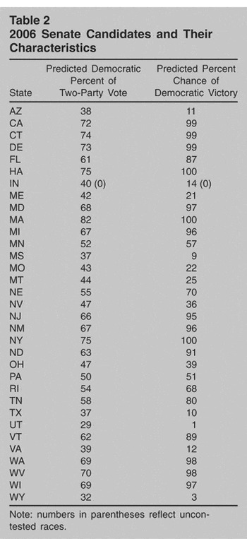
The coefficients associated with the independent variables yielded predicted percentages of the major-party vote that the Democrats should obtain in the 2006 elections. (See column 1 of Table 2.) Barring candidates dropping out, by June 30, 2006, we could code candidates in many Senate contests with certainty. Here is what we found.
2006 Senate Candidates and Their Characteristics

Thirteen states had already held their primaries, making 26 of 66 candidates known. Also, assuming that incumbents would win their primaries, another 16 of the 40 remaining candidates were accounted for. Many states' filing deadlines had passed by June 30. And, there were several instances in which all the contenders shared the same characteristics. There were other instances in which primaries were uncontested. This accounted for 10 of the 24 remaining candidates. Counting Bernie Sanders (I-VT) as a Democrat brought the number of uncertain candidates down to 13. Six of the 13 races had all current candidates running with the same characteristics. As long as new candidates do not decide to contest the primary, the codings for these candidates are known.
This leaves seven out of 66 candidates where uncertainty about candidate characteristics was more problematic than the other cases. In four out of those seven cases, the top two contenders had the same office-holding experience. This meant that the coding would be correct if either of the two candidates won their primaries. Even in these last seven cases there was rarely any real question about who would win the primary. For purposes of coding, candidates for each party were picked based on who would maximize that party's chances at the polls. News accounts we reviewed usually identified the very same candidates as the probable winners of their primaries.
Using the standard error of the estimate, we compute the probability that the Democrat will win each election. (See column 2 of Table 2). In all, Table 2 indicates that in 16 of 33 states there is less than a 90% chance that one party will win the Senate seat. This reflects the fairly competitive nature of Senate elections, as compared to those for the House. The most competitive Senate races for 2006 are those in Pennsylvania (51% chance of a Democratic win), Minnesota (57%), Ohio (39%), Nevada (36%), and Rhode Island (68%). These have been prominently featured in the news as “key races.” The predictions of the model for specific races compares well with the predictions of popular commentators in the media. The top nine states identified by the model as most likely to switch party control include the top eight that Chris Cillizza of the Washington Post's “The Fix” column so identifies in a list of 10.8
See http://blog.washingtonpost.com/thefix/2006/05/the_friday_line_static_senate.html, predictions made on May 12, 2006, accessed July 1, 2006.
CQ classifies Senate races into seven different categories. “Safe Democratic,” “Democratic Favored,” “Leans Democratic,” and “No Clear Favorite,” with three more categories for the Republican side.9
www.cqpolitics.com/risk_rating_senate.html accessed July 1, 2006.
The sixth largest outlier worthy of mention is the case of the Senate race in Pennsylvania, where incumbent Rick Santorum is widely heralded as likely to lose to Democratic challenger Bob Casey. CQ defines this race as “leans Democratic.” Our model gives Santorum a 49% chance of victory. It could be that Santorum's reputation for being a conservative in Pennsylvania is not adequately captured by his roll-call voting record. His involvement in the Terri Schiavo case or his support of President Bush's unpopular Social Security proposals may play especially poorly in Pennsylvania. Challenger Bob Casey's moderate anti-abortion stance may obtain more votes for him in the face of Santorum's more extreme stance on that issue. Another explanation is that the current polls showcased in the popular press are not a good indication of how the election four months from this writing will turn out. Such polls are fraught with problems as forecasting devices (see Green and Gerber 2006, for a listing of some of these). Election night will help resolve this discrepancy.
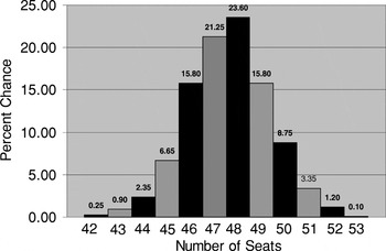
Especially important is assessing the probability that the Democrats will take control of the Senate. The Democrats must win 24 out of 33 races for Senate control. Using the standard error of the estimate from the predicted models, random numbers were generated to simulate 2000 national election outcomes. When added together, these outcomes result in a probability distribution of potential outcomes for the Senate. The probabilities for how many seats the Democrats will have as a result of the 2006 elections are displayed in Figure 1.10
Since Indiana has no Democratic candidate, this election is modeled as a certain Republican victory.

Predicted Percent Chances for Numbers of Democratic Seats
This narrow 95% confidence interval constitutes evidence that the pooled approach utilized here performs better than what we have termed “the aggregate approach.” The 95% confidence interval our model yields is six seats wide. Every other Senate forecasting model we know of yields much larger confidence intervals. For example, the 95% confidence interval that a recent Senate forecasting model yields is around 11 seats wide (Bardwell and Lewis-Beck 2004, 822).11
The standard error of the estimate they report for their model is 2.84. Extending this two standard deviations in either direction means multiplying this number by “4.”
These forecasts also hint at a possible drawback of state by state analyses, such as those used by CQ. In fact, the classic weakness of such state by state analyses, that the state by state calculus does not fully recognize the extent of a nationwide shift, may be playing itself out here. CQ submits that only one state will change hands: Pennsylvania. The only election CQ describes as being too close to call is the 2006 Senate election in Minnesota. This means CQ is predicting a zero- or one-seat change for the 2006 Senate election. Our analysis indicates that at the median prediction, the Democrats will pick up three seats, a much different prediction.
Conclusion
This article presents a new method of predicting Senate elections. In making our predictions, we utilized information about the partisan composition of states, the characteristics of candidates, and whether national conditions favor one party. Estimates from the paper indicate that the 2006 midterm Senate elections will yield a variety of highly competitive races. This finding comports well with that group of Senate races that the media has been emphasizing about the time of this writing. Overall, our model predicts that there is a very slim chance that the Democrats will take control of the Senate: 4.7%.
It should be noted that while our forecast predicts that the Democrats have little chance of taking control of the Senate in 2006, it indicates that they will be in good position for both the 2008 and 2010 elections. In 2008, Republicans must defend 21 seats, while Democrats must defend only 12. If Democrats win just under half of these races, and the forecasts of our model are correct, they will have 52 seats after 2008, a slim majority. The 2010 Senate elections see the Republicans defending 19 seats, the Democrats 15.
Author Bios
Carl Klarner is assistant professor of political science at Indiana State University. He holds a Ph.D. from Texas A&M University. His research interests include campaigns and elections, state politics, and welfare policy, especially as these three subjects pertain to political inequality and reform.
Stan Buchanan teaches and runs the public administration program in the department of political science at Indiana State University, Terre Haute.