1 Introduction
In the frame of the kinetic theory of plasmas, the Vlasov–Poisson system of equations can efficiently solve only some aspects of a huge set of problems. Therefore, it is worth using other approaches to study the dynamics of charged particles and waves in plasmas, which can be considered as alternatives to the quasi-linear theory of the weak turbulence (e.g. Elskens & Escande Reference Elskens and Escande2003; Volokitin & Krafft Reference Volokitin and Krafft2012, Reference Volokitin, Krafft and Zank2016a ,Reference Volokitin and Krafft b ). For example, some are starting from the Vlasov–Poisson system as, for example, the derivation of self-consistent equations of a wave–particle system for studying the nonlinear stage of the interaction of an electron beam with an electrostatic wave in a non-magnetized plasma (Onishchenko et al. Reference Onishchenko, Linetskii, Matsiborko, Shapiro and Shevchenko1970; O’Neil, Winfrey & Malmberg Reference O’Neil, Winfrey and Malmberg1971). Such equations, which were shown to derive from a Hamiltonian (Mynick & Kaufman Reference Mynick and Kaufman1978; Tennyson, Meiss & Morrison Reference Tennyson, Meiss and Morrison1994), have also been obtained within the framework of classical mechanics (Elskens & Escande Reference Elskens and Escande2003).
Further, the generalization of such model to magnetized plasmas, three-dimensional geometry and electromagnetic waves was performed by the authors, who derived the wave–particle and wave–wave Hamiltonians and the corresponding self-consistent systems of equations (Krafft & Volokitin Reference Krafft and Volokitin2004; Volokitin & Krafft Reference Volokitin and Krafft2004; Zaslavsky, Krafft & Volokitin Reference Zaslavsky, Krafft and Volokitin2006; Zaslavsky et al. Reference Zaslavsky, Krafft, Gorbunov and Volokitin2008; Krafft & Volokitin Reference Krafft and Volokitin2010; Volokitin & Krafft Reference Volokitin and Krafft2012; Krafft & Volokitin Reference Krafft and Volokitin2013). The efficiency and the validity of these theoretical models have been proved for different physical situations by comparing the results they provide with experimental observations as well as with numerical simulations based on other methods (e.g. Volokitin, Krafft & Matthieussent Reference Volokitin, Krafft and Matthieussent1997; Krafft, Volokitin & Zaslavsky Reference Krafft, Volokitin and Zaslavsky2005; Krafft & Volokitin Reference Krafft and Volokitin2006; Zaslavsky, Krafft & Volokitin Reference Zaslavsky, Krafft and Volokitin2007; Krafft & Volokitin Reference Krafft and Volokitin2010, Reference Krafft and Volokitin2013). More recently, the authors applied the developed approach to build a model of Langmuir turbulence generated by particle fluxes in inhomogeneous plasmas with random density fluctuations (e.g. Krafft, Volokitin & Krasnoselskikh Reference Krafft, Volokitin and Krasnoselskikh2013; Volokitin et al. Reference Volokitin, Krasnoselskikh, Krafft, Kuznetsov and Zank2013; Krafft et al. Reference Krafft, Volokitin, Krasnoselskikh and Dudok de Wit2014; Krafft, Volokitin & Krasnoselskikh Reference Krafft, Volokitin and Krasnoselskikh2015; Krafft & Volokitin Reference Krafft, Volokitin and Zank2016a ,Reference Krafft and Volokitin b ; Volokitin & Krafft Reference Volokitin and Krafft2016b ). The associated numerical simulations allowed us to describe phenomena predicted by analytical works (e.g. Ryutov Reference Ryutov1970) or observed by several satellites in the heliosphere (e.g. Gurnett & Anderson Reference Gurnett and Anderson1976; Lin et al. Reference Lin, Potter, Gurnett and Scarf1981; Ergun et al. Reference Ergun, Larson, Lin, McFadden, Carlson, Anderson, Muschietti, McCarthy, Parks and Reme1998; Kellogg et al. Reference Kellogg, Goetz, Monson, Bale and Reiner2009; Hess, Malaspina & Ergun Reference Hess, Malaspina and Ergun2011), in particular, by the STEREO and WIND spacecraft (Bougeret et al. Reference Bougeret, Goetz, GoldsteinKaiser, Bale, Kellogg, Maksimovic, Monge, Monson, Astier and Davy2008). More recently, they have been verified by Particle-In-Cell simulations (Thurgood & Tsiklauri Reference Thurgood and Tsiklauri2016).
In the numerical point of view, the use of such methods provides several advantages compared to the kinetic Vlasov–Poisson approach. Indeed, in some of the above cited papers, the authors split the particle velocity distribution into two populations, i.e. the ambient plasma (non-resonant bulk) which supports the wave dispersion and is described by a Vlasovian approach, and the so-called resonant particles which interact with the waves and whose density is much smaller than that of the background plasma. The dynamics of each of these particles is calculated by solving the Newton equations whereas the bulk is represented in the wave fields’ evolution equations by a dielectric constant. Note that such an approach preserves the granular character of the plasma and allows us to avoid the smoothing of the particle velocity distribution and its derivative – as performed in the Vlasov codes – and thus the corresponding loss of information, notably in what concerns the microscopic dynamics. Another important advantage is the possibility to model more easily plasma inhomogeneities. On the other hand, compared to Particle-In-Cell (PIC) codes, the number of particles used in the simulations can be drastically reduced (e.g. compare with Thurgood & Tsiklauri Reference Thurgood and Tsiklauri2016), so that long-time computations in three-dimensional (3-D) magnetized plasmas can be carried out. Moreover, as the system equations have a Hamiltonian form, symplectic integrators give the possibility to use larger time steps and to accelerate strongly the calculations (e.g. Cary & Doxas Reference Cary and Doxas1993).
The paper aims to present recent simulations based on a model developed using the above-mentioned approach and describing the Langmuir turbulence generated by electron beams in inhomogeneous plasmas as the solar wind, where random density fluctuations with average levels up to several per cent of the background plasma density have been detected (Celnikier et al.
Reference Celnikier, Harvey, Jegou, Moricet and Kemp1983). Langmuir waves can be excited via the bump-on-tail instability by beams accelerated in the low corona during solar flares and propagating in the interplanetary plasma. The influence of the randomly fluctuating density inhomogeneities on the wave–particle and wave–wave processes at work has crucial consequences in what concerns the emission of the wave packets, the relaxation of the beam, the generation of fluxes of accelerated particles, the level and the nature of the turbulence and the accompanying nonlinear effects, such as wave decay for example. The long-wavelength density irregularities or the monotonic density gradients inherent to the solar wind plasma can modify significantly the development of such processes, due to the appearance of additional and competing phenomena such as reflection, refraction and scattering (transformation) effects of waves on the density irregularities. Moreover, some studies have stated that density inhomogeneities of the background plasma can be the cause of particle acceleration due to scattering effects (Ryutov Reference Ryutov1970; Kontar & Pecseli Reference Kontar and Pecseli2002; Krafft et al.
Reference Krafft, Volokitin and Krasnoselskikh2013). Indeed, these lead to the transfer of energy from waves of larger wavenumbers
 $k$
to smaller ones, due to the random violations of the resonance conditions between waves and particles. Then the beam can eventually reabsorb part of the energy carried by the waves of larger phase velocities, which leads to the acceleration of electrons with velocities larger than the initial average beam velocity
 $v_{b}$
.
In a previous paper (Krafft & Volokitin Reference Krafft and Volokitin2016b
), the authors have shown how the scattering and the decay processes act together to accelerate beam particles during two successive stages. Indeed, wave transformation on the density fluctuations leads to the appearance of a population of accelerated electrons whose typical velocities lie roughly between
 $v_{b}$
and
 $2v_{b}$
, forming a beam tail that is significantly more dense and energetic, in the considered range of velocities, than the Maxwellian or kappa non-thermal tails of the background plasma velocity distribution. Second, resonant decay of Langmuir waves
 ${\mathcal{L}}$
through the channel
 ${\mathcal{L}}\rightarrow {\mathcal{L}}^{\prime }+{\mathcal{S}}^{\prime }$
produces backscattered Langmuir waves
 ${\mathcal{L}}^{\prime }$
and ion sound waves
 ${\mathcal{S}}^{\prime }$
; if the daughter waves
 ${\mathcal{L}}^{\prime }$
carry enough energy, they can encounter a second decay cascade (SDC) according to
 ${\mathcal{L}}^{\prime }\rightarrow {\mathcal{L}}^{\prime \prime }+{\mathcal{S}}^{\prime \prime }$
, as well as further cascades, until these processes become prohibited by kinematic effects. Then, if the Langmuir waves
 ${\mathcal{L}}^{\prime \prime }$
provided by the second decay cascades have phase velocities
 $v_{\unicode[STIX]{x1D711}}$
lying within the velocity region
 $v_{b}<v_{\unicode[STIX]{x1D711}}\lesssim (2-3)v_{b}$
, they can release part of their energy through Landau damping to this already accelerated electron population and in this way amplify its acceleration, this stage occurring after the saturation of the scattering (transformation) processes.
The aim of the present paper is to understand the influence of the density fluctuations of the background plasma on the dynamics of the Langmuir turbulence generated by electron beams. In particular, one of the aims is to quantify the amount of energy and density carried by the accelerated electron population as a function of the main parameters of the beam as well as of the average level
 $\unicode[STIX]{x0394}n=(\langle (\unicode[STIX]{x1D6FF}n/n_{0})^{2}\rangle )^{1/2}$
of the density fluctuations
 $\unicode[STIX]{x1D6FF}n$
normalized by the average plasma density
 $n_{0}$
. Moreover, the main features of the asymptotic velocity distribution of the beam electrons are studied as a function of these parameters and, in particular, the accelerated tail and the decelerating front and plateau. The results obtained provide relevant results on the mechanism of energy reabsorption by the beam when radiating Langmuir turbulence in solar wind plasmas. Indeed, numerical simulations are performed for parameters typical for solar type III beams and plasmas near 1 AU (e.g. Ergun et al.
Reference Ergun, Larson, Lin, McFadden, Carlson, Anderson, Muschietti, McCarthy, Parks and Reme1998); in the corresponding solar wind regions, the density fluctuations can influence crucially the dynamics and the radiation efficiency of the electron beams generating Langmuir turbulence.
2 Theoretical modelling
The interaction of Langmuir waves with an electron beam in inhomogeneous solar wind plasmas can be studied in 1-D geometry as most of the observed Langmuir wave fields are polarized along the magnetic field lines (Ergun et al.
Reference Ergun, Malaspina, Cairns, Goldman, Newman, Robinson, Eriksson, Bougeret, Briand and Bale2008). As already mentioned in the Introduction, the background plasma of density
 $n_{0}$
is described through the dielectric constant using linear theory whereas only the resonant beam, of density
 $n_{b}\ll n_{0}$
, interacts with the Langmuir fields; it is described by individual particles following the Newton equations (e.g. O’Neil et al.
Reference O’Neil, Winfrey and Malmberg1971; Volokitin & Krafft Reference Volokitin and Krafft2004; Zaslavsky et al.
Reference Zaslavsky, Krafft and Volokitin2006). Moreover the model is based on the Zakharov’s equations (Zakharov Reference Zakharov1972) in which a source term describing the electron beam is introduced; ponderomotive force effects are included even if the density fluctuations considered are existing at the initial state and are not the result of strong turbulence effects. This system can be described by the Hamiltonian
 ${\mathcal{H}}$
when the Landau damping effects can be neglected (Krafft et al.
Reference Krafft, Volokitin and Krasnoselskikh2013)
 $$\begin{eqnarray}\displaystyle {\mathcal{H}} & = & \displaystyle \int _{L}\text{d}z\left(\frac{\unicode[STIX]{x1D70C}}{2}\frac{\left|E\right|^{2}}{8\unicode[STIX]{x03C0}}+\frac{3\unicode[STIX]{x1D706}_{D}^{2}}{16\unicode[STIX]{x03C0}}\left|\frac{\unicode[STIX]{x2202}E}{\unicode[STIX]{x2202}z}\right|^{2}+\frac{n_{0}m_{i}}{2}\left[c_{s}^{2}\unicode[STIX]{x1D70C}^{2}+\left(\frac{\unicode[STIX]{x2202}\unicode[STIX]{x1D6F7}}{\unicode[STIX]{x2202}z}\right)^{2}\right]\right)\nonumber\\ \displaystyle & & \displaystyle +\,\mathop{\sum }_{p}\left(\frac{P_{p}^{2}}{2m_{e}}-e\text{Re}\mathop{\sum }_{k}\frac{\text{i}E_{k}}{k}\text{e}^{-\text{i}\unicode[STIX]{x1D714}_{p}t+\text{i}kz_{p}}\right),\end{eqnarray}$$
where the integral corresponds to the Hamiltonian of the Zakharov equations without any source term, whereas the discrete sum includes the contributions of the kinetic energy of the resonant particles
 $p$
and their energy of interaction with the waves. The electric field is
 $\text{Re}(E\left(z,t\right)\text{e}^{-\text{i}\unicode[STIX]{x1D714}_{p}t})$
, where
 $E\left(z,t\right)=\sum _{k}E_{k}(t)\text{e}^{\text{i}kz}$
is the slowly varying field envelope,
 $\left|\unicode[STIX]{x2202}E/\unicode[STIX]{x2202}t\right|\ll \unicode[STIX]{x1D714}_{p}\left|E\right|$
;
 $E_{k}$
is the Fourier component of
 $E;$
 $z$
is the space coordinate and
 $k$
is the wave vector;
 $\unicode[STIX]{x1D714}_{p}$
and
 $\unicode[STIX]{x1D706}_{D}$
are the electron plasma frequency and Debye length;
 $\unicode[STIX]{x1D714}_{k}=\unicode[STIX]{x1D714}_{p}(1+3k^{2}\unicode[STIX]{x1D706}_{D}^{2}/2)\simeq \unicode[STIX]{x1D714}_{p}$
is the Langmuir wave frequency;
 $\unicode[STIX]{x1D70C}=\unicode[STIX]{x1D6FF}n/n_{0}$
is the normalized ion density perturbation;
 $u$
is the velocity of the ionic population and
 $\unicode[STIX]{x1D6F7}$
is the corresponding hydrodynamic flux potential,
 $u=\unicode[STIX]{x2202}\unicode[STIX]{x1D6F7}/\unicode[STIX]{x2202}z$
;
 $c_{s}$
is the ion acoustic velocity;
 $T_{e}$
and
 $T_{i}$
are the electron and ion temperatures, with
 $T_{e}/T_{i}\gtrsim 3$
;
 $v_{p}$
,
 $z_{p}$
and
 $P_{p}=m_{e}v_{p}$
are the velocity, the position and the generalized momentum of the electron
 $p$
, respectively;
 $L$
is the size of the system and
 $N=Ln_{b}$
is the number of beam particles;
 $-e<0$
is the electron charge;
 $m_{e}$
and
 $m_{i}$
are the electron and ion masses.
The three couples of variables
 $(E/\sqrt{8\unicode[STIX]{x03C0}\unicode[STIX]{x1D714}_{p}},E^{\ast }/\sqrt{8\unicode[STIX]{x03C0}\unicode[STIX]{x1D714}_{p}})$
,
 $(\unicode[STIX]{x1D70C},-n_{0}m_{i}\unicode[STIX]{x1D6F7})~$
and
 $(z_{p},P_{p})$
are the canonical variables of the Hamiltonian
 ${\mathcal{H}}$
, so that the following Hamilton equations
 $$\begin{eqnarray}\displaystyle & & \displaystyle \displaystyle \frac{1}{8\unicode[STIX]{x03C0}\unicode[STIX]{x1D714}_{p}}\frac{\unicode[STIX]{x2202}E}{\unicode[STIX]{x2202}t}=-\text{i}\frac{\unicode[STIX]{x1D6FF}{\mathcal{H}}}{\unicode[STIX]{x1D6FF}E^{\ast }},\quad n_{0}m_{i}\frac{\unicode[STIX]{x2202}\unicode[STIX]{x1D6F7}}{\unicode[STIX]{x2202}t}=-\frac{\unicode[STIX]{x1D6FF}{\mathcal{H}}}{\unicode[STIX]{x1D6FF}\unicode[STIX]{x1D70C}},\end{eqnarray}$$
 $$\begin{eqnarray}\displaystyle & & \displaystyle \displaystyle v_{p}=\frac{\text{d}z_{p}}{\text{d}t}=\frac{\unicode[STIX]{x2202}{\mathcal{H}}}{\unicode[STIX]{x2202}P_{p}},\quad \frac{\text{d}P_{p}}{\text{d}t}=-\frac{\unicode[STIX]{x2202}{\mathcal{H}}}{\unicode[STIX]{x2202}z_{p}},\end{eqnarray}$$
where
 $\unicode[STIX]{x1D6FF}$
is the functional derivative, provide the complete set of the (non-normalized) model’s equations, that is
 $$\begin{eqnarray}\displaystyle & \displaystyle m_{e}\frac{\text{d}v_{p}}{\text{d}t}=-e\text{Re}\mathop{\sum }_{k}E_{k}\text{e}^{\text{i}kz_{p}-\text{i}\unicode[STIX]{x1D714}_{k}t}, & \displaystyle\end{eqnarray}$$
 $$\begin{eqnarray}\displaystyle & \displaystyle \text{i}\frac{\unicode[STIX]{x2202}E}{\unicode[STIX]{x2202}t}+\frac{3\unicode[STIX]{x1D706}_{D}^{2}}{2}\unicode[STIX]{x1D714}_{p}\frac{\unicode[STIX]{x2202}^{2}E}{\unicode[STIX]{x2202}z^{2}}-\frac{\unicode[STIX]{x1D714}_{p}\unicode[STIX]{x1D70C}}{2}E=4\unicode[STIX]{x03C0}\text{i}en_{b}\mathop{\sum }_{k}\frac{\unicode[STIX]{x1D714}_{p}}{k}J_{k}\text{e}^{\text{i}kz}, & \displaystyle\end{eqnarray}$$
 $$\begin{eqnarray}\displaystyle & \displaystyle \frac{\unicode[STIX]{x2202}^{2}\unicode[STIX]{x1D70C}}{\unicode[STIX]{x2202}t^{2}}-c_{s}^{2}\frac{\unicode[STIX]{x2202}^{2}\unicode[STIX]{x1D70C}}{\unicode[STIX]{x2202}z^{2}}=\frac{\unicode[STIX]{x2202}^{2}}{\unicode[STIX]{x2202}z^{2}}\frac{\left|E\right|^{2}}{16\unicode[STIX]{x03C0}m_{i}n_{0}}, & \displaystyle\end{eqnarray}$$
 $$\begin{eqnarray}\displaystyle & \displaystyle \frac{\unicode[STIX]{x2202}u}{\unicode[STIX]{x2202}z}=-\frac{\unicode[STIX]{x2202}\unicode[STIX]{x1D70C}}{\unicode[STIX]{x2202}t}, & \displaystyle\end{eqnarray}$$
where
 $$\begin{eqnarray}J_{k}=\frac{1}{N}\mathop{\sum }_{p}\text{e}^{\text{i}\unicode[STIX]{x1D714}_{k}t-ikz_{p}}.\end{eqnarray}$$
In the Fourier space, equations (2.5)–(2.7) can be written as
 $$\begin{eqnarray}\displaystyle & \displaystyle \text{i}\left(\frac{\unicode[STIX]{x2202}}{\unicode[STIX]{x2202}t}-\unicode[STIX]{x1D6FE}_{k}^{\left(e\right)}\right)E_{k}=\frac{3}{2}\unicode[STIX]{x1D714}_{p}k^{2}\unicode[STIX]{x1D706}_{D}^{2}E_{k}+\frac{\unicode[STIX]{x1D714}_{p}}{2}\left(\unicode[STIX]{x1D70C}E\right)_{k}+\text{i}\frac{4\unicode[STIX]{x03C0}e\unicode[STIX]{x1D714}_{p}n_{b}}{k}J_{k}, & \displaystyle\end{eqnarray}$$
 $$\begin{eqnarray}\displaystyle & \displaystyle \frac{\unicode[STIX]{x2202}u_{k}}{\unicode[STIX]{x2202}t}-2\unicode[STIX]{x1D6FE}_{k}^{\left(i\right)}u_{k}=-\text{i}kc_{s}\left(\unicode[STIX]{x1D70C}_{k}+\frac{\left(\left|E\right|^{2}\right)_{k}}{16\unicode[STIX]{x03C0}m_{i}n_{0}c_{s}^{2}}\right), & \displaystyle\end{eqnarray}$$
 $$\begin{eqnarray}\displaystyle & \displaystyle \frac{\unicode[STIX]{x2202}\unicode[STIX]{x1D70C}_{k}}{\unicode[STIX]{x2202}t}=-\text{i}kc_{s}u_{k}, & \displaystyle\end{eqnarray}$$
where we added afterwards the damping factors
 $\unicode[STIX]{x1D6FE}_{k}^{\left(e\right)}$
and
 $\unicode[STIX]{x1D6FE}_{k}^{\left(i\right)}$
in order to take into account damping effects on the electrons and the ions, respectively;
 $u_{k}$
and
 $\unicode[STIX]{x1D70C}_{k}$
are the Fourier components of
 $u$
and
 $\unicode[STIX]{x1D70C}$
, respectively. Indeed, even if in the present description the background (bulk) plasma is not modelled using individual particles, non-thermal tails of its velocity distribution can play a role as they lie in the velocity range where wave–particle interaction processes take place. The numerical solution of (2.8–2.10) is performed according to the scheme described in the appendix of Krafft et al. (Reference Krafft, Volokitin and Krasnoselskikh2013).
Waves and particles are distributed initially in a periodic simulation box of size
 $L=10\,000-30\,000\unicode[STIX]{x1D706}_{D}$
. The beam velocity distribution is modelled by a Maxwellian function and the resonant electrons are distributed uniformly in space. Even if the resonant electrons travel several times along the periodic simulation box during simulations performed over long time periods, one can consider that at each of their passage they interact with Langmuir waves with new spectra and phases, as the time scale for a significant variation of the Langmuir turbulence is shorter than the time of travel of electrons through the box. Initially, 1024–2048 plasma waves of random phases and small amplitudes are distributed in the Fourier space, with wave vectors
 $-k_{max}<k<k_{max}$
, where
 $k_{max}\unicode[STIX]{x1D706}_{D}\simeq 0.2{-}0.3$
. The space and time resolutions ensuring the trustworthiness of the physical results obtained are, depending on the simulations, approximately
 $2{-}10\unicode[STIX]{x1D706}_{D}$
and
 $0.01{-}0.02\unicode[STIX]{x1D714}_{p}^{-1}$
, respectively.
Numerical simulations are carried out for parameters typical for solar type III beams and plasmas near 1 AU (e.g. Ergun et al.
Reference Ergun, Larson, Lin, McFadden, Carlson, Anderson, Muschietti, McCarthy, Parks and Reme1998); the beam drift and thermal velocities
 $v_{b}$
and
 $\unicode[STIX]{x0394}v_{b}$
satisfy
 $10\lesssim v_{b}/v_{T}\lesssim 50$
and
 $0.05\lesssim \unicode[STIX]{x0394}v_{b}/v_{b}\lesssim 0.1$
, where
 $v_{T}$
is the electron thermal velocity of the background plasma. The beam density
 $n_{b}$
is much smaller than the plasma density
 $n_{0}\simeq 5\times 10^{6}$
m
 $^{-3}$
, i.e.
 $5\times 10^{-6}\lesssim n_{b}/n_{0}\lesssim 5\times 10^{-5}$
. The ambient plasma temperature and the electron Debye length are around
 $T_{e}\simeq 10$
–20 eV and
 $\unicode[STIX]{x1D706}_{D}\sim 15$
m. Below
 $\unicode[STIX]{x1D714}_{p}t$
,
 $v/v_{T}$
and
 $E_{k}/\sqrt{4\unicode[STIX]{x03C0}n_{0}T_{e}}$
are the normalized values of time, velocity and spectral electric field.
Initially, the profiles of the plasma density fluctuations
 $\unicode[STIX]{x1D6FF}n/n_{0}$
are set with characteristic spatial scales
 $\unicode[STIX]{x1D706}_{n}\simeq 300$
–
 $2000\unicode[STIX]{x1D706}_{D}$
much larger than the typical Langmuir wavelengths, and with average levels
 $\unicode[STIX]{x0394}n=(\langle (\unicode[STIX]{x1D6FF}n/n_{0})^{2}\rangle )^{1/2}$
varying approximately from
 $0.001$
to
 $0.04$
, in order to describe realistic solar wind conditions. These long-wavelength fluctuations’ profiles are evolving self-consistently with the waves and the beam during the simulations. The existence of a threshold
 $\unicode[STIX]{x0394}n_{s}=\unicode[STIX]{x1D6FC}(v_{T}/v_{b})^{2}$
(
 $\unicode[STIX]{x1D6FC}\simeq 2-3$
) was stated in previous works (e.g. Krafft et al.
Reference Krafft, Volokitin and Krasnoselskikh2013); when
 $\unicode[STIX]{x0394}n\ll \unicode[STIX]{x1D6FC}\left(v_{T}/v_{b}\right)^{2}$
, the system evolves as in a quasi-homogeneous plasma and, when
 $\unicode[STIX]{x0394}n\gtrsim \unicode[STIX]{x1D6FC}\left(v_{T}/v_{b}\right)^{2}$
, the presence of plasma density fluctuations impacts significantly on the Langmuir turbulence and its interactions with the beam.
3 Numerical simulations: beam acceleration by Langmuir turbulence
The dynamics of the system is governed by the beam instability, which gives rise to Langmuir wave emission, and by various nonlinear effects, among which wave transformation on inhomogeneities and resonant wave–wave coupling are most important. During the beam relaxation stage, its velocity distribution
 $f(v)$
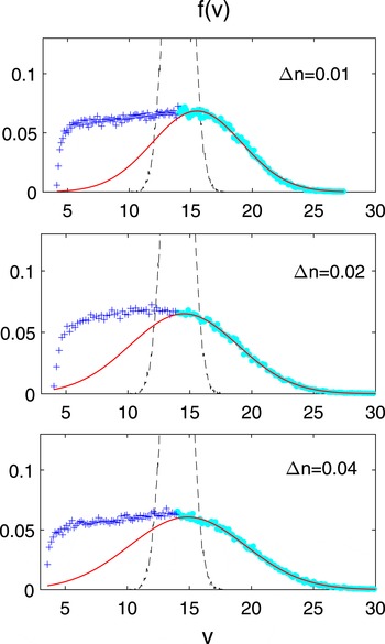
widens toward lower as well as higher velocities, forming both a tail of accelerated electrons and a decelerating plateau. Figure 1 shows
 $f(v)$
for different
 $\unicode[STIX]{x0394}n\gtrsim \unicode[STIX]{x0394}n_{s}$
, i.e.
 $\unicode[STIX]{x0394}n=0.01$
,
 $0.02$
, and
 $0.04$
, at
 $\unicode[STIX]{x1D714}_{p}t=0$
and asymptotic times around
 $\unicode[STIX]{x1D714}_{p}t\simeq 150\,000$
. One observes that the asymptotic distributions of the accelerated beam tail can be interpolated by Gaussian functions centred near
 $v\simeq v_{b}$
, with thermal velocities
 $\unicode[STIX]{x0394}v_{b}+\unicode[STIX]{x0394}V$
weakly depending on
 $\unicode[STIX]{x0394}n$
;
 $\unicode[STIX]{x0394}V>0$
is the increase of thermal velocity with respect to the initial beam distribution. Note that the fits are obtained using least squares’ methods with
 $R$
-square values
 $R_{sq}\gtrsim 99.5\,\%$
. In these examples, the acceleration of particles is almost strictly due to the transformation of Langmuir waves on the randomly varying density fluctuations, during which energy transfer from larger to smaller
 $k$
takes place, allowing the reabsorption of wave energy by the beam tail, i.e. by particles with velocities
 $v>v_{b}$
. Indeed, when inhomogeneities are present, the successive decay cascades are less effective at producing Langmuir waves with significant intensities (Krafft et al.
Reference Krafft, Volokitin and Krasnoselskikh2015), compared to the case of homogeneous plasmas.
Velocity distribution
 $f(v)$
of the beam for
 $\unicode[STIX]{x0394}n=0.01$
,
 $0.02$
and
 $0.04$
, at
 $\unicode[STIX]{x1D714}_{p}t=0$
(black dashed lines) and
 $\unicode[STIX]{x1D714}_{p}t\simeq 150\,000$
(blue crosses and cyan points). Points provided by the simulations (crosses and points) have been fitted by Gaussian distributions (red solid lines), taking into account only the velocities
 $v$
larger than the initial beam velocity
 $v_{b}$
. The points excluded from the fits and forming the decelerating plateau are represented by blue crosses. Velocities are normalized by the electron thermal velocity
 $v_{T}$
.

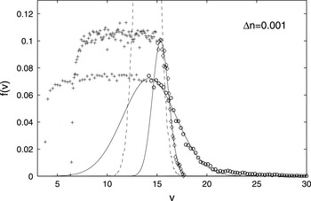
If one examines
 $f(v)$
for a quasi-homogeneous plasma with
 $\unicode[STIX]{x0394}n=0.001\ll \unicode[STIX]{x0394}n_{s}$
at three different times in figure 2 (at
 $t=0$
, at the time
 $\unicode[STIX]{x1D714}_{p}t=47\,500$
when the wave transformation processes on inhomogeneities have reached saturation and at
 $\unicode[STIX]{x1D714}_{p}t\simeq 170\,000$
, when the SDC process is already at work), one can see that particle acceleration due to wave transformation effects is very weak (as
 $\unicode[STIX]{x0394}n$
is very weak). However, another acceleration process takes place, due to Langmuir waves produced by the second cascade of the decay of the beam-driven Langmuir waves, which is more effective in quasi-homogeneous plasmas than in inhomogeneous ones. Interpolating
 $f(v)$
with Gaussians is however difficult in this case, and fits with
 $R_{sq}\gtrsim 99.5\,\%$
can be performed only with Gaussians centred at
 $v\simeq v_{b}+\unicode[STIX]{x0394}v_{b}$
(otherwise, when centred at
 $v\simeq v_{b}$
, sigmoidal functions exhibit better fits). Moreover, one can see some deviations from the Gaussian behaviour in the beam tail distribution at
 $\unicode[STIX]{x1D714}_{p}t\simeq 170\,000$
(e.g. around the normalized velocity
 $v\simeq 22$
), as the tail is more dense than a Gaussian one and resembles more a kappa-type tail. Indeed, in this case, the SDC process is not fully saturated, which should be the most important reason for the non-Gaussian character of the tail; at this stage, the energy spectrum of the Langmuir waves coming from the second decay cascade is significantly varying in the velocity range considered, due to local resonant energy exchanges between the waves and the tail particles.
Velocity distribution
 $f(v)$
of the beam for a quasi-homogeneous plasma with
 $\unicode[STIX]{x0394}n=0.001$
, at (i)
 $\unicode[STIX]{x1D714}_{p}t=0$
(dashed line), (ii)
 $\unicode[STIX]{x1D714}_{p}t=47\,500$
(crosses and diamonds) and (iii)
 $\unicode[STIX]{x1D714}_{p}t\simeq 170\,000$
(crosses and circles). Points provided by the simulations have been fitted by Gaussian distributions (solid lines) for the beam accelerated tail, taking into account only velocities
 $v$
larger than the initial beam velocity
 $v_{b}$
. The points excluded from these fits and representing the decelerated plateau are labelled by crosses. Velocities are normalized by the electron thermal velocity
 $v_{T}$
.

The Gaussian character of the beam tails at well-established wave saturation is connected to the fact that, in this velocity region
 $v>v_{b}$
, the velocity diffusion coefficients
 $D(v)$
of particles have been shown to be quasi-constant at saturation times (Volokitin & Krafft Reference Volokitin, Krafft and Zank2016a
,Reference Volokitin and Krafft
b
). Note that the quasi-linear theory of weak turbulence in homogeneous plasmas predicts such behaviour in the range of velocity where waves do not exchange a significant amount of energy with particles. Moreover, when the processes of wave transformation on inhomogeneities and of second decay cascade have reached a full saturation (i.e. when energy exchanges between waves and particles become very weak at asymptotic times), the coefficients
 $D(v)$
can become quasi-constant at
 $v>v_{b}$
even if the plasma is not homogeneous. However, when one of these processes is not fully saturated (as in figure 2 at
 $\unicode[STIX]{x1D714}_{p}t\simeq 170\,000$
for the second decay cascade), the beam accelerated tail deviates locally from a Gaussian shape.
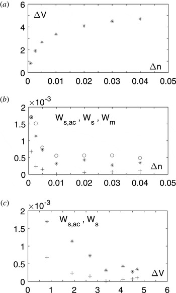
(a) Thermal velocity
 $\unicode[STIX]{x0394}V$
gained by the accelerated tail of the beam with respect to the initial beam distribution, as a function of
 $\unicode[STIX]{x0394}n$
. (b) Variation of the maximum of Langmuir wave energy density
 $W_{m}$
(circles), the saturated energy densities of all the Langmuir waves,
 $W_{s}$
(stars), and of the Langmuir waves with phase velocities
 $v_{\unicode[STIX]{x1D711}}>v_{ac}$
,
 $W_{s,ac}$
(crosses), as a function of
 $\unicode[STIX]{x0394}n$
. (c) Variation of
 $W_{s}$
(stars) and
 $W_{s,ac}$
(crosses) with
 $\unicode[STIX]{x0394}V$
. The density threshold is
 $\unicode[STIX]{x0394}n_{s}\simeq 0.01$
. All the variables are normalized.

The increase of thermal velocity
 $\unicode[STIX]{x0394}V$
is shown as a function of
 $\unicode[STIX]{x0394}n$
in figure 3(a), when both acceleration processes are taken indistinctly into account. For each
 $\unicode[STIX]{x0394}n$
,
 $\unicode[STIX]{x0394}V$
is calculated at a time when wave saturation is reached. The error bars of
 $\unicode[STIX]{x0394}V$
are not indicated on the figure as their maximal size corresponds approximately to that of the markers. These errors result mainly from the fact that, at asymptotic times, the central velocities of the fitted Gaussians can be shifted from
 $v_{b}$
to
 $v_{b}\pm \unicode[STIX]{x1D6FC}v_{b}$
, with
 $\unicode[STIX]{x1D6FC}\simeq 0.01{-}0.05$
depending on
 $\unicode[STIX]{x0394}n$
. The figure reveals that
 $\unicode[STIX]{x0394}V\simeq \unicode[STIX]{x0394}v_{b}$
for small values of
 $\unicode[STIX]{x0394}n$
(e.g.
 $\unicode[STIX]{x0394}n\simeq 0.001$
), and that
 $\unicode[STIX]{x0394}V$
increases with
 $\unicode[STIX]{x0394}n$
, reaching
 $\unicode[STIX]{x0394}V\simeq 4\unicode[STIX]{x0394}v_{b}$
when
 $\unicode[STIX]{x0394}n=0.04$
. For
 $\unicode[STIX]{x0394}n\lesssim \unicode[STIX]{x0394}n_{s}$
(here
 $\unicode[STIX]{x0394}n_{s}\simeq 0.01$
), the heating of
 $f(\text{v})$
is mainly due to the second decay cascade and for
 $\unicode[STIX]{x0394}n\gtrsim \unicode[STIX]{x0394}n_{s}$
, to the wave transformation effects on the inhomogeneities.
We can expect that
 $\unicode[STIX]{x0394}V$
should not increase significantly for
 $\unicode[STIX]{x0394}n\gtrsim 0.04$
due to the following reasons: (i) Langmuir wave decay becomes very rare for
 $\unicode[STIX]{x0394}n\gtrsim 0.04$
(e.g. Krafft et al.
Reference Krafft, Volokitin and Krasnoselskikh2015), so that the probability for the SDC process to occur in such a case is very small; (ii) a large part of the Langmuir energy emitted by the beam is absorbed by waves of negative
 $k$
due to reflection effects on large density humps, so that the transfer of energy to smaller positive
 $k$
as a result of transformation effects on the density inhomogeneities should not noticeably increase; (iii) as
 $\unicode[STIX]{x0394}n=0.04\gtrsim \unicode[STIX]{x0394}n_{s}$
for beams with
 $v_{b}/v_{T}\gtrsim 8$
, increasing
 $\unicode[STIX]{x0394}n$
above
 $0.04$
for such beams would not significantly modify the level of saturation of the Langmuir energy emitted (e.g. Krafft & Volokitin Reference Krafft and Volokitin2013), so that the available energy should be roughly the same for any
 $\unicode[STIX]{x0394}n\gtrsim 0.04$
and, consequently, the energy actually absorbed by the tail electrons should not grow.
When looking at the waves’ behaviour, one observes in figure 3(b) that the maximum of Langmuir wave energy density
 $W_{m}$
, the saturated energy densities of all the Langmuir waves and of those with phase velocities
 $v_{\unicode[STIX]{x1D711}}$
lying in the acceleration region
 $v_{ac}=v_{b}+\unicode[STIX]{x0394}v_{b}\lesssim v\lesssim (2-3)v_{b}$
,
 $W_{s}$
and
 $W_{s,ac}=W_{s}(v_{\unicode[STIX]{x1D711}}>v_{ac})$
respectively, decrease when
 $\unicode[STIX]{x0394}n$
increases. Here the saturated wave levels are measured at asymptotic times. For
 $\unicode[STIX]{x0394}n\gtrsim \unicode[STIX]{x0394}n_{s}$
, the level of all the energy densities depends weakly on
 $\unicode[STIX]{x0394}n$
. Note that
 $W_{s,ac}$
is noticeably lower than
 $W_{s}$
: when
 $\unicode[STIX]{x0394}n\lesssim \unicode[STIX]{x0394}n_{s}$
, it is due to the fact that no significant amount of energy is transferred to the waves with
 $v_{\unicode[STIX]{x1D711}}>v_{ac}$
as wave transformation effects are weak (even if
 $\unicode[STIX]{x0394}V$
has a noticeable value due to the SDC process) and, when
 $\unicode[STIX]{x0394}n\gtrsim \unicode[STIX]{x0394}n_{s}$
, it results from the fact that, at the asymptotic times considered, the Langmuir waves with
 $v_{\unicode[STIX]{x1D711}}>v_{ac}$
have lost part of their energy gained due to transformation processes and have released it through damping to the particles with
 $v\gtrsim v_{ac}$
. One can observe that
 $W_{s,ac}$
and
 $W_{s}$
decrease when
 $\unicode[STIX]{x0394}V$
increases (figure 3
c); indeed, for very low saturation levels (i.e. for large
 $\unicode[STIX]{x0394}n$
), the energy carried by the waves has been partly absorbed by the particles which are accelerated.
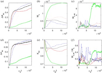
Time variation of different characteristics of the population of accelerated particles, for
 $\unicode[STIX]{x0394}n=0.001$
(thick green lines),
 $0.005$
(dotted red lines),
 $0.02$
(thin black lines) and
 $0.04$
(dashed blue lines): (a) kinetic energy
 $\unicode[STIX]{x0394}K_{ac}$
gained by the accelerated electrons, (d) density
 $\unicode[STIX]{x0394}n_{ac}$
gained by the accelerated electrons, (b) Langmuir wave energy density
 $W_{L}$
, (e) kinetic energy
 $K_{tot}$
carried by the beam, (c) fraction
 $W_{L,ac}$
of the energy density
 $W_{L}$
carried by the Langmuir waves with
 $v_{\unicode[STIX]{x1D711}}>v_{ac}$
, (f) ratio
 $W_{L,ac}/W_{L}$
. All variables are normalized.

Let us now determine the kinetic energy
 $\unicode[STIX]{x0394}K_{ac}$
and the density
 $\unicode[STIX]{x0394}n_{ac}$
gained by the population of accelerated particles as a function of time, for different values of
 $\unicode[STIX]{x0394}n$
. Figure 4 shows the time variation of the total normalized beam kinetic energy
 $K_{tot}=K_{tot}(t)/K_{0}$
(
 $K_{0}$
is the initial beam kinetic energy), the normalized gains
 $\unicode[STIX]{x0394}K_{ac}=(K_{ac}(v>v_{ac},t)\!-K_{ac}(v>v_{ac},t=0))/K_{0}$
and
 $\unicode[STIX]{x0394}n_{ac}=(n_{ac}(v>v_{ac},t)\!-n_{ac}(v>v_{ac},t=0))$
 $/n_{b}$
, the normalized Langmuir wave energy density
 $W_{L}$
, its fraction
 $W_{L,ac}=W_{L}(v_{\unicode[STIX]{x1D711}}>v_{ac})$
carried by the Langmuir waves with
 $v_{\unicode[STIX]{x1D711}}>v_{ac}=v_{b}+\unicode[STIX]{x0394}v_{b}$
and the ratio
 $W_{L,ac}/W_{L}$
. For sake of readability, we show here only the time variations for
 $\unicode[STIX]{x0394}n=0.001$
,
 $0.005$
,
 $0.02$
and
 $0.04$
. Note that the reader can refer to previous works of the authors (e.g. Krafft et al.
Reference Krafft, Volokitin and Krasnoselskikh2015; Krafft & Volokitin Reference Krafft, Volokitin and Zank2016a
,Reference Krafft and Volokitin
b
) to observe the procession of the
 ${\mathcal{L}}$
waves to smaller
 $k$
via the two mechanisms at work, as described below.
First, one can observe the growth of
 $W_{L}$
, which is accompanied by the decrease of
 $K_{tot}$
; wave emission is more effective when
 $\unicode[STIX]{x0394}n$
is low and becomes strongly reduced when
 $\unicode[STIX]{x0394}n$
grows. For
 $\unicode[STIX]{x0394}n=0.04$
(respectively
 $\unicode[STIX]{x0394}n=0.001$
), the beam has lost only 5 % (respectively 30 %) of its initial energy. Significant wave energy growth and accompanying loss of beam energy occurs mainly for
 $\unicode[STIX]{x1D714}_{p}t\lesssim 50\,000$
, whereas the saturation stages begin near
 $\unicode[STIX]{x1D714}_{p}t\sim 50\,000$
. During this time range, and for
 $\unicode[STIX]{x0394}n>0.001$
, the transfer of energy from the beam-driven Langmuir waves
 ${\mathcal{L}}$
to Langmuir modes of smaller
 $k$
takes place, due to the wave transformation effects, leading to a strong increase of
 $\unicode[STIX]{x0394}n_{ac}$
and
 $\unicode[STIX]{x0394}K_{ac}$
. Then
 $\unicode[STIX]{x0394}K_{ac}/K_{0}$
and
 $\unicode[STIX]{x0394}n_{ac}/n_{b}$
begin to saturate but continue to slowly increase. This is due
 $~$
to the fact that the transformation effects are not totally achieved, even if they weaken with respect to time increase. For example, for
 $\unicode[STIX]{x0394}n=0.04$
(blue curves)
 $W_{L,ac}$
decreases slowly during a long range of time (approximately during
 $100\,000\unicode[STIX]{x1D714}_{p}^{-1}$
, beginning from
 $\unicode[STIX]{x1D714}_{p}t\simeq 50\,000$
); meanwhile
 $W_{L,ac}/W_{L}~$
reaches its maximum around
 $0.65$
during the stage when
 $W_{L}$
is growing (
 $\unicode[STIX]{x1D714}_{p}t\lesssim 50\,000$
) and continues to exhibit peaks at large times, which can reach up to
 $0.4$
(figure 4
f). On the other hand, for
 $\unicode[STIX]{x0394}n=0.001$
, the small growth of
 $\unicode[STIX]{x0394}n_{ac}$
and
 $\unicode[STIX]{x0394}K_{ac}$
is almost entirely due to the appearance of the SDC process, which starts to be effective near
 $\unicode[STIX]{x1D714}_{p}t\sim 50\,000$
.
Let us now discuss the time variations of
 $W_{L,ac}$
and
 $W_{L,ac}/W_{L}$
for the cases when
 $\unicode[STIX]{x0394}n<0.04$
, i.e.
 $\unicode[STIX]{x0394}n=0.001$
,
 $0.005$
and
 $0.02$
. For
 $\unicode[STIX]{x1D714}_{p}t\gtrsim 50\,000$
both
 $W_{L,ac}$
and
 $W_{L,ac}/W_{L}$
are growing, reaching an average value which decreases slowly during a late range of time, as shown for
 $\unicode[STIX]{x0394}n=0.001$
(green curves). This is due to the appearance of Langmuir waves
 ${\mathcal{L}}^{\prime \prime }$
coming from the second decay cascade, which have phase velocities
 $v_{\unicode[STIX]{x1D711}}\gtrsim v_{ac}$
; those contribute strongly to the enhancement of the density
 $\unicode[STIX]{x0394}n_{ac}$
and the kinetic energy
 $\unicode[STIX]{x0394}K_{ac}$
of the electron population already accelerated due to transformation effects. For
 $\unicode[STIX]{x0394}n=0.02$
(black curves), two phenomena take place at
 $\unicode[STIX]{x1D714}_{p}t\gtrsim 50\,000$
, i.e. the wave transformation effects (however weaker than for
 $\unicode[STIX]{x1D714}_{p}t\lesssim 50\,000$
) and the SDC process, occurring only at
 $\unicode[STIX]{x1D714}_{p}t\gtrsim 50\,000$
. As shown in the figure 4
f, more
 $\unicode[STIX]{x0394}n$
is large (resp. small) and more the fraction
 $W_{L,ac}/W_{L}$
of wave energy provided by the transformation (resp. the SDC) processes to waves with
 $v_{\unicode[STIX]{x1D711}}\gtrsim v_{ac}$
is large.
So the behaviour of the curves at small
 $\unicode[STIX]{x0394}n$
is very different from the other ones: for
 $\unicode[STIX]{x0394}n\ll \unicode[STIX]{x0394}n_{s}\sim 0.01$
, the beam loses a large portion of its kinetic energy which produces eventually a high level of Langmuir turbulence (see e.g. the green curves). When
 $\unicode[STIX]{x0394}n\gtrsim \unicode[STIX]{x0394}n_{s}$
, the efficiency of Langmuir wave emission is significantly reduced due to the violation of the resonance conditions between waves and particles and to the reabsorption of the waves’ energy by the beam; at large
 $\unicode[STIX]{x0394}n$
, the beam has lost eventually only a small portion of its energy (i.e. 5 % for
 $\unicode[STIX]{x0394}n=0.04$
), explaining its possible propagation over very long distances.
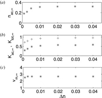
Variation with
 $\unicode[STIX]{x0394}n$
of different characteristics of the population of accelerated particles, at asymptotic time. (a) Density
 $n_{ac,\infty }$
normalized by the beam density; (b) kinetic energy
 $K_{ac,\infty }$
normalized by the initial beam energy (stars), with the total normalized kinetic energy of the beam
 $K_{tot,\infty }$
(crosses); (c) maximum velocity
 $v_{m,\infty }$
reached by the accelerated particles, in units of
 $v_{b}$
.

Figure 5 shows the variation with
 $\unicode[STIX]{x0394}n$
of
 $n_{ac,\infty }=n_{ac}(v>v_{ac},t=\infty )/n_{b}$
,
 $K_{ac,\infty }=K_{ac}(v>v_{ac},t=\infty )/K_{0}$
,
 $K_{tot,\infty }=K_{tot}(t=\infty )/K_{0}$
and of the maximum velocity
 $v_{m,\infty }=v_{max}(t=\infty )/v_{b}$
of the beam tail’s particles. One can see that
 $n_{ac,\infty }$
and
 $K_{ac,\infty }$
increase with
 $\unicode[STIX]{x0394}n$
, showing two ranges of
 $\unicode[STIX]{x0394}n$
with different behaviours. For
 $\unicode[STIX]{x0394}n\lesssim \unicode[STIX]{x0394}n_{s}\sim 0.01$
,
 $n_{ac,\infty }$
and
 $K_{ac,\infty }$
are strongly dependent on
 $\unicode[STIX]{x0394}n$
, exhibiting quasi-linear dependences
 $n_{ac,\infty }\propto \unicode[STIX]{x0394}n$
and
 $K_{ac,\infty }\propto \unicode[STIX]{x0394}n$
. This is no more true when
 $\unicode[STIX]{x0394}n\gtrsim \unicode[STIX]{x0394}n_{s}$
, for which
 $n_{ac,\infty },K_{ac,\infty }\simeq \text{cst}$
. The maxima reached are
 $n_{ac,\infty }\simeq 0.3$
and
 $K_{ac,\infty }\simeq 0.6$
, showing that the density and the kinetic energy of the accelerated particles can eventually reach large fractions of the initial beam density and energy. The variation of
 $K_{tot,\infty }$
with
 $\unicode[STIX]{x0394}n$
shows that for small values as
 $\unicode[STIX]{x0394}n\simeq 0.001$
, the beam loses 30 % of its energy while for
 $\unicode[STIX]{x0394}n\simeq 0.04$
it loses only 5 % of it, the transformation processes preventing the beam from releasing energy and causing the decrease of the turbulence level that it generates. The beam is decelerating but, due to the formation of a tail of accelerated particles which can reabsorb part of the energy it loses, the net energy lost (i.e. radiated into wave energy) is very small when inhomogeneities are present. Through such reabsorption the beam can conserve its kinetic energy during a much more long time when propagating in plasmas with random density fluctuations than in homogeneous plasmas. Finally, the variation of
 $v_{m,\infty }$
reveals that the accelerated tail can extend up to almost three times the initial beam velocity, and that this value is not strongly depending on
 $\unicode[STIX]{x0394}n$
.
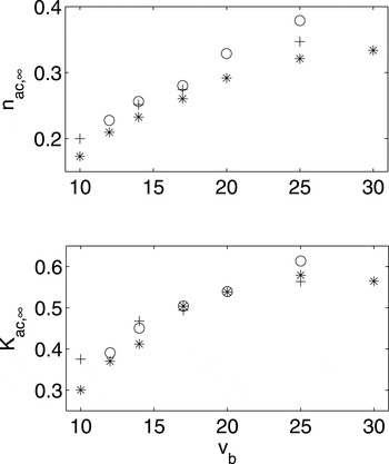
Variation of
 $n_{ac,\infty }$
and
 $K_{ac,\infty }$
with the normalized initial beam velocity
 $v_{b}$
, for
 $\unicode[STIX]{x0394}n=0.01$
(circles),
 $0.02$
(stars) and
 $0.03$
(crosses).

Figure 6 shows the variation of
 $n_{ac,\infty }$
and
 $K_{ac,\infty }$
as a function of the initial beam velocity
 $v_{b}$
(normalized by
 $v_{T}$
), between
 $v_{b}=10$
and
 $v_{b}=30$
; note that this range is typical for the beams actually existing in the solar wind regions of the foreshock and the type III solar bursts’ sources near 1 AU. In the whole, the density and the kinetic energy of the accelerated population increase with
 $v_{b}$
, more strongly within the range
 $10\lesssim v_{b}\lesssim 20$
than the range
 $20\lesssim v_{b}\lesssim 30$
in what concerns the energy. The values of
 $n_{ac,\infty }$
and
 $K_{ac,\infty }$
vary only slightly (of the order of 15 %) when
 $\unicode[STIX]{x0394}n$
grows from
 $0.01$
to
 $0.03$
. Thus, for a given inhomogeneous plasma, a beam with a larger velocity presents a more dense and energetic population of accelerated particles than a beam of smaller velocity; the ratio can reach up to a factor two when
 $v_{b}$
varies from
 $10$
to
 $30$
. When the beam is moderately energetic (
 $10\lesssim v_{b}\lesssim 20$
),
 $\unicode[STIX]{x0394}n$
does not strongly impact on
 $n_{ac,\infty }$
and
 $K_{ac,\infty }$
, if
 $\unicode[STIX]{x0394}n\gtrsim \unicode[STIX]{x0394}n_{s}$
.
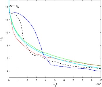
Time variation of the decelerating front velocity
 $u_{f}$
of the beam velocity distribution, for
 $\unicode[STIX]{x0394}n=0.001$
(solid green curve),
 $0.005$
(dotted red curve),
 $0.02$
(dashed black curve) and
 $0.04$
(dotted-dashed blue curve). The theoretical prediction provided by the quasi-linear theory of weak turbulence is shown by a solid cyan line.

Finally, it is worth determining the variation with
 $\unicode[STIX]{x0394}n$
of the decelerating front velocity
 $u_{f}$
of
 $f(\text{v})$
. Figure 7 shows
 $u_{f}(t)$
(normalized by
 $v_{T}$
) for
 $\unicode[STIX]{x0394}n=0.001$
,
 $0.005$
,
 $0.02$
and
 $0.04$
, together with its theoretical prediction provided by the quasi-linear theory (QLT) of weak turbulence in homogeneous plasmas (Vedenov, Velikhov & Sagdeev Reference Vedenov, Velikhov and Sagdeev1961). As expected, for a quasi-homogeneous plasma
 $\left(\unicode[STIX]{x0394}n=0.001\right)$
, the variation of
 $u_{f}(t)$
is in agreement with the QLT (compare the cyan and the green curves). The behaviour of
 $u_{f}(t)$
becomes strongly modified within the time range
 $\unicode[STIX]{x1D714}_{p}t\lesssim 20\,000$
for
 $\unicode[STIX]{x0394}n=0.02$
and
 $\unicode[STIX]{x1D714}_{p}t\lesssim 40\,000$
for
 $\unicode[STIX]{x0394}n=0.04$
; more larger is
 $\unicode[STIX]{x0394}n$
, more larger
 $u_{f}$
and more slower its time variation. So, if
 $\unicode[STIX]{x0394}n>\unicode[STIX]{x0394}n_{s}$
, the front deceleration is decreased in the range of time when wave transformation processes occur and lead to particle acceleration. A change of behaviour of
 $u_{f}(t)$
occurs at the time corresponding to the saturation of the growth of the density and the kinetic energy carried by the accelerated electrons (approximately
 $\unicode[STIX]{x1D714}_{p}t\simeq 30\,000$
for
 $\unicode[STIX]{x0394}n=0.02$
and
 $\unicode[STIX]{x1D714}_{p}t\simeq 40\,000$
for
 $\unicode[STIX]{x0394}n=0.04$
); further (
 $\unicode[STIX]{x1D714}_{p}t\gtrsim 40\,000$
), all the front velocities follow roughly the QLT variation (cyan curve), even if
 $u_{f}$
is noticeably smaller when the plasma is inhomogeneous. This can be explained by the fact that at asymptotic times, the exchanges of energy between waves and particles become very small as well as weakly dependent on
 $\unicode[STIX]{x0394}n$
(see also the above figures).
4 Conclusion
The paper studies the influence of the background plasma density fluctuations on the dynamics of the Langmuir turbulence generated by electron beams, for parameters typical for solar type III beams and plasmas near 1 AU. A self-consistent Hamiltonian model based on the Zakharov and the Newton equations is used, which presents several advantages compared to the Vlasov approach.
In a quasi-homogeneous plasma, i.e. for
 $\unicode[STIX]{x0394}n\ll \unicode[STIX]{x0394}n_{s}$
, the beam loses a large portion of its kinetic energy (up to half, depending on the beam parameters), generating a high level of Langmuir turbulence. Beam particles can be accelerated, but due to the second cascade of the wave decay process only, the wave transformation effects being very weak as
 $\unicode[STIX]{x0394}n\ll \unicode[STIX]{x0394}n_{s}$
. At asymptotic times, the accelerated electron population can carry up to 30 % of the initial beam energy, due to the transfer of energy from the beam-driven Langmuir waves to Langmuir waves coming from the second decay cascade, which have phase velocities larger than the beam initial velocity; thus, it can eventually reabsorb an appreciable part of the energy lost by the beam.
When the plasma is inhomogeneous, i.e.
 $\unicode[STIX]{x0394}n\gtrsim \unicode[STIX]{x0394}n_{s}$
, the efficiency of Langmuir wave emission is significantly reduced due to the presence of density fluctuations and to the reabsorption of wave energy by the beam. The beam releases only a small portion of its energy (i.e. 5 % for
 $\unicode[STIX]{x0394}n=0.04$
), which explains its ability to propagate over very long distances in the plasma. The tail of accelerated electrons can carry up to 60 % of the initial beam energy as a result of wave transformation effects and of second decay cascade processes; it can reabsorb Langmuir energy due to resonant wave–particle interactions and thus prevent the decelerating beam from losing energy. As a consequence the beam can conserve a large part of its initial kinetic energy during a much longer time when propagating in plasmas with random density fluctuations than in homogeneous plasmas.
The net gains and losses of energy of the beam and the waves have been calculated as a function of the average level of plasma density fluctuations and the beam drift velocity. The mechanism of energy reabsorption by beams radiating Langmuir turbulence in solar wind plasmas has been shown to produce efficient electron acceleration. Moreover the results obtained should shed light on the dynamics and the radiation efficiency of particle fluxes and beams originating from various sources and propagating in space plasmas involving randomly fluctuating density or magnetic inhomogeneities, provided that they emit wave turbulence through resonant wave–particle interactions. The process of reabsorption allows beams to radiate moderate levels of wave turbulence over large distances and to transport energy far from their emission sources. These two circumstances should be taken into account for the interpretation of space and astrophysical observations.
Acknowledgements
The authors acknowledge the Institut du Développement et des Ressources en Informatique Scientifique (IDRIS, Orsay, France) for the computational ressources. This work was granted access to the HPC resources of IDRIS under the allocation 2013- i2013057017 made by GENCI. This work has been done within the LABEX Plas@par project, and received financial state aid managed by the Agence Nationale de la Recherche, as part of the programme ‘Investissements d’avenir’ under the reference ANR-11-IDEX-0004-02. C.K. acknowledges the ‘Programme National Soleil Terre’ (PNST) of the Centre National d’Etudes Spatiales (CNES, France).