1 Introduction
Hydraulic fractures (HF) are tensile (mode I) fractures propagating in a material under pre-existing compressive stress driven by fluid injection. The propagation of these fluid-driven fractures in an impermeable material are governed by the interplay between elastic deformation, lubrication fluid flow within fracture and the creation of new surfaces. Notably, the competition between the dissipation associated with viscous flow and that associated with fracturing the material governs how the fracture propagates: either in the viscosity dominated or toughness dominated regime. The transition between these two regimes is now well understood. Reference solutions do exist for simple fracture geometries (Detournay Reference Detournay2016) and laboratory experiments do compare well with theoretical predictions (Lecampion et al. Reference Lecampion, Desroches, Jeffrey and Bunger2017; Xing et al. Reference Xing, Yoshioka, Adachi, El-Fayoumi and Bunger2017).
However, in some circumstances, the basic assumption of a laminar viscous flow inside the propagating fracture is clearly challenged. This is notably the case during slickwater fracturing treatments that aim to stimulate the production of gas wells in low permeability reservoirs. In such a type of fracturing operation, water is injected at a very high rate in order to compensate for the low viscosity of water and to obtain sufficient fracture width for proppant placement. High injection rate of a low viscosity fluid leads to a Reynolds number up to
 $10^{5}$
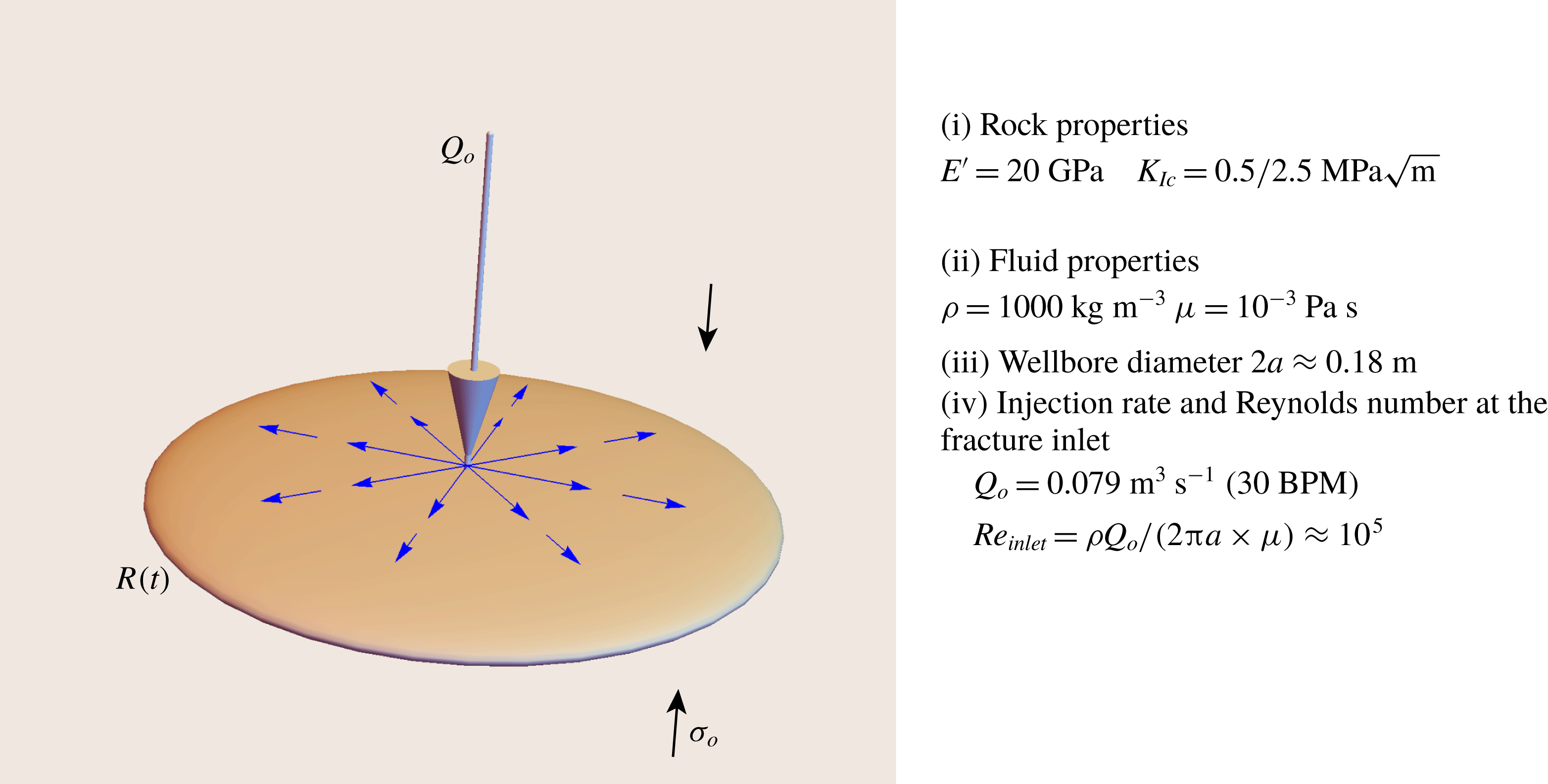
at the fracture inlet for a radial fracture geometry (see figure 1), clearly above the laminar–turbulent transition for parallel plate type flow.
Sketch of a radial hydraulic fracture (radius
 $R(t)$
, width
 $w(r,t)$
and net pressure
 $p(r,t)=p_{f}(r,\,t)-\unicode[STIX]{x1D70E}_{o}$
) propagating in an elastic impermeable medium (left). Example of material properties and injection parameters for a slickwater treatment resulting in large Reynolds number at the fracture inlet. The chosen injection rate is an upper bound (twice as large as the typical value of
 $Q_{o}=15$
barrels per minute (BPM)).

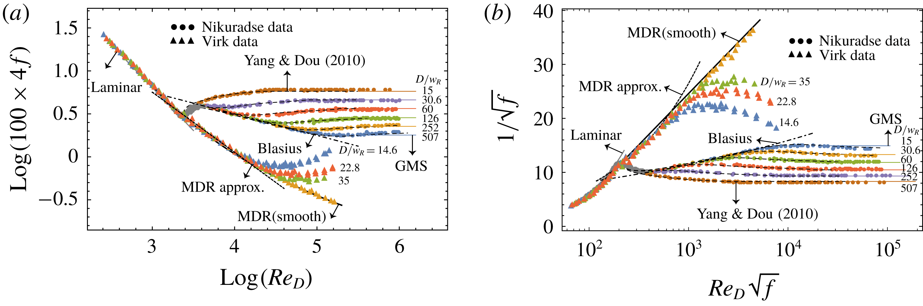
The influence of turbulent flow on hydraulic fracture propagation has been investigated in the context of magmatic dykes (Emerman, Turcotte & Spence Reference Emerman, Turcotte and Spence1986; Lister & Kerr Reference Lister and Kerr1991), glacier drainage (Tsai & Rice Reference Tsai and Rice2010, Reference Tsai and Rice2012) as well as industrial hydraulic fracturing (Perkins & Kern Reference Perkins and Kern1961). Fracture growth solutions under turbulent conditions have been obtained recently for simple geometries (plane strain, radial, blade-like fractures: see Zia & Lecampion (Reference Zia and Lecampion2017), Zolfaghari, Meyer & Bunger (Reference Zolfaghari, Meyer and Bunger2017), Zolfaghari & Bunger (Reference Zolfaghari and Bunger2018a ,Reference Zolfaghari and Bunger b ), Zolfaghari, Dontsov & Bunger (Reference Zolfaghari, Dontsov and Bunger2018)). The influence of turbulence was also studied early on with respect to gas-driven fracture propagation (Nilson Reference Nilson1981) where it was noted that the flow will transition from turbulent to laminar condition inside the fracture as one moves closer to the fracture tip. The structure of the near-tip behaviour of a propagating hydraulic fracture accounting for the laminar–turbulent transition was quantitatively investigated recently (Dontsov Reference Dontsov2016a ), providing a rationale for the quantification of the near-tip laminar region. All these contributions have used the large body of literature on turbulent flow of water in pipes and rectangular duct/parallel plates to account for the laminar–turbulent flow transition via the evolution of the friction factor with Reynolds number and fracture relative roughness (see figure 2).
Unfortunately, the energy required to pump plain water at a high rate from the surface down the wellbore to the target perforated zone for fracturing (kilometres away) leads to prohibitive costs (e.g. large number of pumping trucks). This is even more true as it is typical to try to propagate several hydraulic fractures at once, therefore multiplying the surface injection rate accordingly. In order to be able to perform such injections down the wellbore at a realistic economical cost, heavy weight drag reducing agents must be added to water resulting in a fracturing fluid coined slickwater. The addition to water of heavy molecular weight polymers, albeit in a small amount, is well known to drastically modify the transition to turbulence and to significantly lower down the associated friction factor (Toms Reference Toms1948; Virk et al. Reference Virk, Merrill, Mickley, Smith and Mollo-Christensen1967). The long polymer chain reduces the formation of eddies, allowing for a reduction of up to 90 % in the energy required for a pumping operation. The effect of drag reduction agent on turbulence is well characterised in pipe flow. We refer to the classical review of Virk (Reference Virk1975) and the recent one of White & Mungal (Reference White and Mungal2008) for more details. An important point is that the impact on turbulent flow actually saturates at rather small concentration of the polymer additive, leading to a so-called maximum drag reduction (MDR) asymptote in the turbulent regime, as can be seen on figure 2.
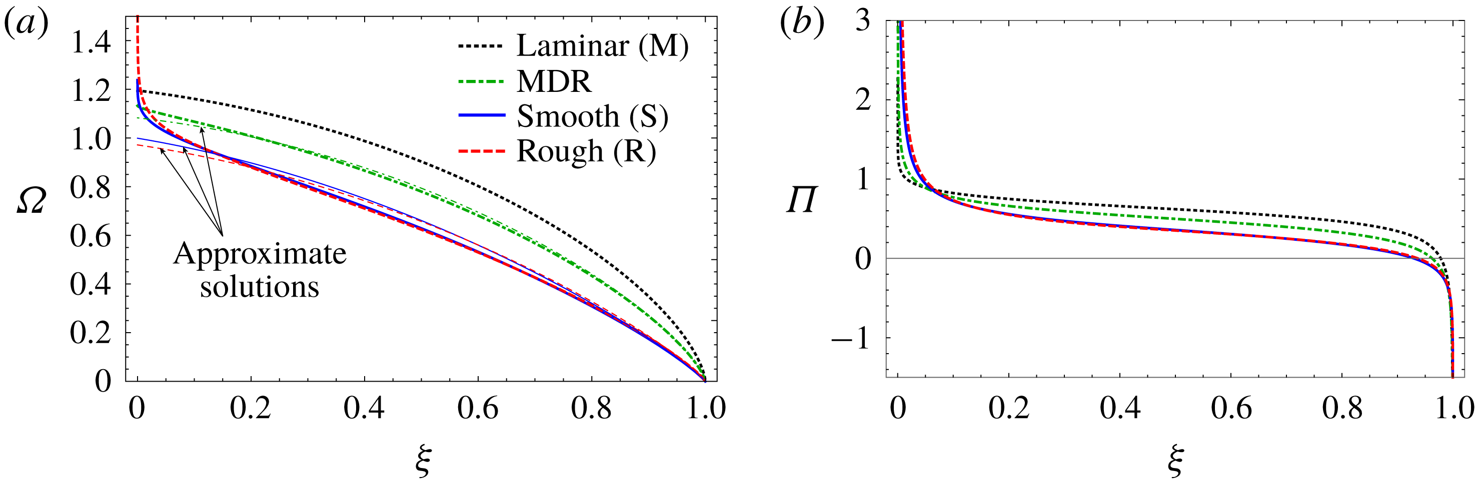
(a) Evolution of the friction factor
 $f$
in a circular pipe as a function of the Reynolds number
 $Re_{D_{eq}}=\unicode[STIX]{x1D70C}\overline{v}D/\unicode[STIX]{x1D707}$
and relative roughness
 $2k_{R}/D$
, where
 $k_{R}$
is the characteristic roughness scale (and
 $D/2$
the pipe radius). The experimental data of Nikuradse (Reference Nikuradse1950) for pipes of different roughness are plotted together with the expressions for the laminar friction
 $f=16/Re_{D_{eq}}$
valid for
 $Re_{D_{eq}}<2300$
, the smooth turbulent Blasius friction
 $4f=0.316Re^{-1/4}$
(dash-dotted black line) and the turbulent rough Glaucker–Manning–Strickler
 $4f=0.143(2k_{R}/D)^{1/3}$
(solid dashed line). The predictions of the model of Yang & Dou (Reference Yang and Dou2010) are also plotted as thin dashed lines. Experimental data of Virk (Reference Virk1971, Reference Virk1975) at maximum drag reduction are also plotted, together with the MDR asymptote (full solid lines) and the approximation given by (2.14). (b) The same data are also shown in a Prandtl–Kármán diagram (the variation of
 $1/\sqrt{f}$
against
 $Re_{D_{eq}}\sqrt{f}$
).

The main goal of this contribution is to investigate how the use of drag reduction agents combined with a large injection rate impacts hydraulic fracture propagation. We focus on both the finite radial (penny-shaped) fracture geometry and the near-tip/semi-infinite hydraulic fracture problem. The radial geometry is notably relevant for the early time of growth of a hydraulic fracture from a horizontal well before the fracture reaches the bounding layers (Lecampion & Desroches Reference Lecampion and Desroches2015). The near-tip problem on the other hand encapsulates all the nonlinearities of hydraulic fracturing (Garagash & Detournay Reference Garagash and Detournay2000; Garagash, Detournay & Adachi Reference Garagash, Detournay and Adachi2011). Its multiscale structure notably quantifies the energy dissipated in different processes, both in the injected fluid and in the solid (Garagash Reference Garagash and Borodich2009). Although, we focus most of our discussion on the use of drag reducing agents, we also discuss the case of plain water (without additives) in order to highlight similarities and differences.
A number of limiting solutions will be obtained based on the recognition that all limiting turbulent flow regimes can actually be re-expressed in a generalised form of the Poiseuille lubrication law similar to the one for power-law fluids. This important point was first noted by Tsai & Rice (Reference Tsai and Rice2010) for the case of rough turbulent flow and is, as we shall see, actually valid for all limiting flow regimes for plain water (rough, smooth turbulent) as well as slickwater (at maximum drag reduction). This thus allows us to adapt the method of solutions initially developed for such coupled hydraulic fracture problems: notably the one of Savitski & Detournay (Reference Savitski and Detournay2002) for the case of a radial hydraulic fracture propagating in the viscosity dominated regime under the assumption of laminar flow.
2 Radial hydraulic fracture: problem formulation
The main assumptions of our penny-shaped hydraulic fracture model are similar to previous contributions: (i) the material is assumed to be homogeneous elastic and isotropic, (ii) the fracture propagation is assumed to be quasi-static and is assumed to obey the well-established concepts of linear elastic fracture mechanics, (iii) the fluid is injected at a constant rate from a point source at the fracture centre, (iv) the material is assumed to be impermeable and (v) the fluid front is assumed to coincide with the fracture tip (which is the case for sufficiently deep fractures, see Garagash & Detournay (Reference Garagash and Detournay2000) for more discussion).
2.1 Governing equations
For such a planar axisymmetric pure opening mode fracture of radius
 $R(t)$
, quasi-static elasticity reduces to the following boundary integral equation between the fracture aperture
 $w(r,t)$
and the distribution of net loading
 $p(r,t)$
(Sneddon & Lowengrub Reference Sneddon and Lowengrub1969; Cleary & Wong Reference Cleary and Wong1985):
 $$\begin{eqnarray}\displaystyle w(r,t)=\frac{8R(t)}{\unicode[STIX]{x03C0}E^{\prime }}\int _{0}^{1}G(r/R(t),\unicode[STIX]{x1D709})p(\unicode[STIX]{x1D709}R(t),t)\,\text{d}\unicode[STIX]{x1D709}, & & \displaystyle\end{eqnarray}$$
where
 $E^{\prime }=E/(1-\unicode[STIX]{x1D708}^{2})$
is the plane-strain Young’s modulus, and
 $p(r,t)=p_{f}(r,t)-\unicode[STIX]{x1D70E}_{o}$
is the net pressure loading on the fracture faces, i.e. the fluid pressure in excess of the in situ compressive stress
 $\unicode[STIX]{x1D70E}_{o}$
normal to the fracture plane. The elastic kernel
 $G$
is recalled in appendix A for completeness. For such a penny-shaped fracture, the stress intensity factor can be expressed using the following weight function integral (Rice Reference Rice1972)
 $$\begin{eqnarray}\displaystyle K_{I}=\frac{2}{\sqrt{\unicode[STIX]{x03C0}R}}\int _{0}^{R}\frac{p(r,t)}{\sqrt{R^{2}-r^{2}}}r\,\text{d}r. & & \displaystyle\end{eqnarray}$$
The quasi-static fracture propagation condition stipulates that the mode I stress intensity factor
 $K_{I}$
is always equal to the material fracture toughness
 $K_{Ic}$
. In other words,
 $K_{I}=K_{Ic}$
in (2.2).
This penny-shaped fracture is driven by a point injection of a fluid at its centre. Under the assumption of an impermeable rock, for an incompressible fluid, the width-averaged fluid mass conservation in the fracture reduces to the following continuity equation in axisymmetry for
 $r\in [0,R(t)]$
:
 $$\begin{eqnarray}\displaystyle \frac{\unicode[STIX]{x2202}w}{\unicode[STIX]{x2202}t}+\frac{1}{r}\frac{\unicode[STIX]{x2202}}{\unicode[STIX]{x2202}r}(rwv)=0, & & \displaystyle\end{eqnarray}$$
where
 $v$
denotes the width-averaged radial fluid velocity and
 $q=wv$
is the corresponding fluid flux. The point-source injection condition at the fracture centre (neglecting the wellbore radius
 $a$
compared to the fracture size) is given by
 $$\begin{eqnarray}\displaystyle \lim _{r\rightarrow 0}2\unicode[STIX]{x03C0}r\,w(r,t)v(r,t)=Q_{o}. & & \displaystyle\end{eqnarray}$$
Correspondingly, at the fracture tip, the flow rate
 $q=wv$
as well as the fracture opening are zero (Detournay & Peirce Reference Detournay and Peirce2014),
 $$\begin{eqnarray}\displaystyle q(R(t),t)=0,\quad w(R(t),t)=0. & & \displaystyle\end{eqnarray}$$
The width-averaged fluid momentum equation for such a parallel plate axisymmetric flow is given by
 $$\begin{eqnarray}\displaystyle \unicode[STIX]{x1D70C}\left(\frac{\unicode[STIX]{x2202}v}{\unicode[STIX]{x2202}t}+v\frac{\unicode[STIX]{x2202}v}{\unicode[STIX]{x2202}r}\right)=-\frac{\unicode[STIX]{x2202}p_{f}}{\unicode[STIX]{x2202}r}-\frac{2}{w}\unicode[STIX]{x1D70F}_{w}, & & \displaystyle\end{eqnarray}$$
where
 $\unicode[STIX]{x1D70C}$
is the fluid density and
 $\unicode[STIX]{x1D70F}_{w}$
is the average wall shear stress typically expressed as
 $$\begin{eqnarray}\displaystyle \unicode[STIX]{x1D70F}_{w}=f\left(Re,\frac{k_{R}}{w}\right)\times \frac{\unicode[STIX]{x1D70C}v|v|}{2}. & & \displaystyle\end{eqnarray}$$
The fluid velocity has to be understood as a local time average in the presence of turbulence. The averaged wall shear stress is a function of the Fanning friction factor
 $f$
which depends on the local Reynolds number
 $Re$
, the relative roughness of the flow geometry
 $k_{R}/w$
and the shape of the cross-section perpendicular to the flow direction. In our case, it is natural to define the Reynolds number as
 $$\begin{eqnarray}\displaystyle Re=\frac{\unicode[STIX]{x1D70C}wv}{\unicode[STIX]{x1D707}}. & & \displaystyle\end{eqnarray}$$
It is important to note that the Reynolds number at a given point varies inside the fracture as both the fracture width and fluid velocity vary in space and time. The Reynolds number (2.8) notably decreases from the fracture inlet to the fracture tip as the fracture width
 $w$
tends to zero near the tip. As a result, a laminar region is always expected to be present near the tip, albeit reducing to a boundary layer. For flow in a thin channel/fracture, it can be shown that the inertial terms on the left-hand side of the balance of momentum (2.6) scale as
 $R_{e}\times w/R$
(e.g. Szeri Reference Szeri2010) which remains typically small for a fracture as
 $w/R\ll 1$
. For a liquid, inertial terms are thus negligible compared to the viscous terms on the right-hand side (more precisely, they only play a role at extremely early times, see Garagash (Reference Garagash2006) and Zia & Lecampion (Reference Zia and Lecampion2017) for more discussion). In the following, we neglect inertial terms, such that the width-averaged balance of momentum reduces to the following relation between pressure gradient, fluid velocity and friction factor:
 $$\begin{eqnarray}\displaystyle v\times |v|=-\frac{w}{\unicode[STIX]{x1D70C}\times f\left(Re,{\displaystyle \frac{k_{R}}{w}}\right)}\frac{\unicode[STIX]{x2202}p_{f}}{\unicode[STIX]{x2202}r}. & & \displaystyle\end{eqnarray}$$
2.2 Friction factor with and without drag reducing additives
The evolution of the friction factor as a function of the Reynolds number and relative roughness
 $f(Re,k_{R}/w)$
is well known for circular pipes (see figure 2). A large number of phenomenological relations for the evolution of the friction factor have been proposed. All these phenomenological expressions are based on steady-state experimental data of pressure drop as a function of velocity. They are thus valid only when the time–space average of inertial terms is indeed negligible.
The transition to turbulence as well as the effect of pipe roughness on the wall shear stress can be clearly seen on Moody and Prandtl–Kármán type plot (figure 2). The effect of the addition of heavy molecular weight polymers has also been extensively studied due to its drastic effect on turbulence (see figure 2). The long polymer chain induces viscoelasticity, reducing turbulence significantly (see Virk (Reference Virk1975) and White & Mungal (Reference White and Mungal2008) and references therein). The effect saturates at relatively low polymer concentration: a maximum drag reduction asymptote (MDR) emerges in turbulent flow. Such a maximum drag reduction is therefore always obtained at a reasonable cost in industrial hydraulic fracturing operations.
2.2.1 Friction in fractures
In order to apply the phenomenological relations originally derived for pipe flow to the parallel plate type flow, Jones (Reference Jones1976) suggests obtaining the characteristic dimension
 $D_{eq}$
used to determine the Reynolds number for parallel plate flow by matching the laminar friction (which is given analytically by Poiseuille law for a parallel plate flow) with the expression for a circular pipe in the laminar flow regime
 $f_{laminar}=16\,Re_{D_{eq}}^{-1}$
. This ensures that the proper friction is recovered in the laminar regime for a parallel plate flow. The predictions of friction in the turbulent regime using
 $Re_{D_{eq}}$
in the expressions of friction for a circular pipe agrees very well with experimental data for rectangular ducts of different aspect ratios (Jones Reference Jones1976). In the case of parallel plate type flow, in the laminar regime, the mean velocity is given by Poiseuille law (see e.g. Lamb Reference Lamb1932)
 $v=-(w^{2}/12\unicode[STIX]{x1D707})(\unicode[STIX]{x2202}p/\unicode[STIX]{x2202}r)$
. Writing
 $f_{laminar}=16\times Re_{D_{eq}}^{-1}=16\unicode[STIX]{x1D707}/(\unicode[STIX]{x1D70C}D_{eq}v)$
in the laminar regime, the laminar equivalent pipe diameter is simply obtained by comparing (2.9) with the previous equation as
 $D_{eq}=(4/3)w$
. We therefore use
 $D_{eq}$
in the definition of the Reynolds number entering the expressions for the friction factor for circular pipes. In other words, following Jones (Reference Jones1976), we use the following definition for the equivalent laminar pipe Reynolds number
 $Re_{D_{eq}}$
:
 $$\begin{eqnarray}\displaystyle Re_{D_{eq}}={\textstyle \frac{4}{3}}Re, & & \displaystyle\end{eqnarray}$$
where
 $Re$
corresponds to the Reynolds number (2.8) defined with the mean fracture width as the characteristic flow dimension. Such a choice allows us to directly use the different friction models derived for circular pipe while ensuring that we recover the proper expression in the laminar flow regime. As can be seen in figure 2, the transition to turbulent flow starts around
 $Re_{D}\approx 2200$
in a pipe, which gives for parallel plate flow a critical number
 ${\mathcal{R}}_{c}\approx 2200\times 3/4\approx 1650$
– a value only slightly lower than the one obtained experimentally for a plane Poiseuille flow in a rectangular duct (Jones Reference Jones1976).
Note that we can also rewrite the lubrication law (2.9), following Dontsov (Reference Dontsov2016a )
 $$\begin{eqnarray}\displaystyle v=-\frac{w^{2}}{12\unicode[STIX]{x1D707}\times \tilde{f}\left(Re_{D_{eq}},{\displaystyle \frac{k_{R}}{w}}\right)}\frac{\unicode[STIX]{x2202}p_{f}}{\unicode[STIX]{x2202}r}, & & \displaystyle\end{eqnarray}$$
where
 $\tilde{f}(Re_{D_{eq}},k_{R}/w)=f((4/3)Re,k_{R}/w)/f_{laminar}$
.
2.2.2 Limiting turbulent regimes
The friction factor
 $f$
depends on both the local value of the Reynolds number and relative roughness of the fracture, as depicted in figure 2. Although empirical models exist to somehow capture the complete evolution of
 $f$
, it is interesting to focus on limiting regimes for friction: laminar, turbulent rough, turbulent smooth etc. Explicit expressions for the friction factor exist in these different limiting turbulent regimes, and can be subsequently used to derive limiting solutions for hydraulic fracture growth.
Turbulent rough regime
At very large Reynolds numbers (
 $Re\gg 10^{5}$
), friction for plain water is solely governed by the relative roughness
 $k_{R}/w$
, where
 $k_{R}$
is the roughness scale. In that rough turbulent limiting regime, the friction factor evolves according to the Gauckler–Manning–Strickler scaling (Tsai & Rice Reference Tsai and Rice2010; Zia & Lecampion Reference Zia and Lecampion2017)
 $$\begin{eqnarray}\displaystyle f=f_{R}\times \left(\frac{k_{R}}{w}\right)^{\unicode[STIX]{x1D6FC}_{R}},\quad \unicode[STIX]{x1D6FC}_{R}=1/3,\quad f_{R}=2^{1/3}\times 0.143/4, & & \displaystyle\end{eqnarray}$$
where the factor
 $f_{R}$
allows for a perfect match with the experimental data (Nikuradse Reference Nikuradse1950).
Turbulent smooth regime
The turbulent regime for plain water in smooth pipes (where roughness is negligible) is well captured by the Blasius (Reference Blasius1913) scaling (see figure 2)
 $$\begin{eqnarray}\displaystyle f=f_{B}Re_{D_{eq}}^{-n_{B}},\quad n_{B}=1/4,\quad f_{B}=0.316/4, & & \displaystyle\end{eqnarray}$$
which is an empirical formula with a response similar to the Prandtl–Kármán theoretical predictions for smooth pipes.
Turbulent maximum drag reduction asymptote
As already mentioned, the addition of a friction reducer drastically changes the turbulent behaviour (Virk Reference Virk1975). When friction reducers are added in a sufficient concentration, the maximum drag reduction asymptote is reached. In that so-called MDR limit, the turbulent flow – even in a rough pipe, as can be seen from figure 2 – can be well captured by the following expression for Reynolds number in the range
 $[10^{3}{-}3\times 10^{4}]$
 $$\begin{eqnarray}\displaystyle f=f_{mdr}Re_{D_{eq}}^{-n_{mdr}},\quad n_{mdr}\approx 7/10,\quad f_{mdr}\approx 1.78. & & \displaystyle\end{eqnarray}$$
We will use this expression for simplicity in the following. It is interesting to point out that the last two regimes have a similar power-law relation between the friction factor and the Reynolds number, i.e.
 $f=f_{o}Re^{-n}$
.
2.2.3 Generalised Poiseuille law for limiting regimes
Combining the definition for the equivalent Reynolds number (2.10) and the relation between the width-averaged velocity and pressure gradient (2.9), it is possible to rewrite the general equation (2.9) for any limiting flow regime previously discussed as
 $$\begin{eqnarray}\displaystyle v\times |v|^{m-1}=-\frac{w^{n+1}}{c}\frac{\unicode[STIX]{x2202}p}{\unicode[STIX]{x2202}r}, & & \displaystyle\end{eqnarray}$$
where both the exponents
 $m$
and
 $n$
as well as the constant
 $c$
depend on the limiting flow regimes. For the laminar case, we simply have
 $c=12\unicode[STIX]{x1D707}$
,
 $m=1$
and
 $n=1$
. In the limiting turbulent flow regimes, these parameters take the following values:
(i) Turbulent rough – Gauckler–Manning–Strickler scaling
 $f=f_{R}\times (k_{R}/w)^{1/3}$
(2.12): (2.16a-c )$$\begin{eqnarray}\displaystyle c=f_{R}k_{R}^{1/3}\unicode[STIX]{x1D70C},\quad n=1/3,\quad m=2. & & \displaystyle\end{eqnarray}$$
(ii) Turbulent regimes where
$f=f_{o}Re^{-n}$
: (2.17a-c )$$\begin{eqnarray}\displaystyle c=\underbrace{(4/3)^{-n}f_{o}}_{f_{o}^{\prime }}\unicode[STIX]{x1D707}^{n}\unicode[STIX]{x1D70C}^{1-n},\quad m=2-n,\quad f_{o}^{\prime }=(4/3)^{-n}f_{o}. & & \displaystyle\end{eqnarray}$$


The case of a smooth turbulent regime (Blasius scaling) as well as the case of the maximum drag reduction asymptote both fall under this form where
 $f=f_{o}Re^{-n}$
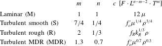
. Table 1 summarises the parameters of these three turbulent regimes in the generalised lubrication equation (2.15).
Generalised lubrication parameters of the different flow regimes. We use the notation
 $f_{o}^{\prime }=(4/3)^{-n}f_{o}$
for short;
 $f_{o}\approx 1.78$
for the MDR approximation, and
 $f_{o}\approx 0.316/4$
for turbulent smooth.

We therefore can use the general form of the averaged velocity/pressure gradient relation (2.15) to solve for the different limiting flow regimes in a similar way. Moreover, as first noted by Tsai & Rice (Reference Tsai and Rice2010) for the turbulent rough case, this general lubrication relation (2.15) is actually exactly similar in its mathematical form to the Poiseuille law for a power-law rheology (with
 $m=n$
) for which
 $c$
and
 $n$
are the power-law consistency and fluid index respectively. One can therefore take advantage of the solution of hydraulic fracture problems obtained for a power-law rheology: notably, the zero toughness near-tip solution derived by Desroches et al. (Reference Desroches, Detournay, Lenoach, Papanastasiou, Pearson, Thiercelin and Cheng1994), as well as its extension to power-law fluid (Madyarova & Detournay Reference Madyarova and Detournay2004) for a penny-shaped hydraulic fracture propagating in a zero toughness medium, originally derived for a Newtonian fluid and laminar flow (Savitski & Detournay Reference Savitski and Detournay2002). We shall see that few adaptations are necessary to extend this zero toughness power-law laminar solution to the turbulent limiting regimes.
2.3 Inlet behaviour
The constant point-source injection (2.4) directly results in a
 $1/r$
singularity for the Reynolds number
 $Re=\unicode[STIX]{x1D70C}wv/\unicode[STIX]{x1D707}$
as it can be rewritten as
 $\lim _{r\rightarrow 0}2\unicode[STIX]{x03C0}rRe=\unicode[STIX]{x1D70C}Q_{o}/\unicode[STIX]{x1D707}$
. Obviously, in practice, injection always occurs from a finite wellbore (of radius
 $a$
) such that the inlet Reynolds number is limited to
 $Re_{max}=\unicode[STIX]{x1D70C}Q_{o}/(2\unicode[STIX]{x03C0}a\times \unicode[STIX]{x1D707})$
(see figure 1). Note that this also is the case for numerical evaluation, when using a finite grid to model the growth of a planar three-dimensional hydraulic fracture (Dontsov & Peirce Reference Dontsov and Peirce2017). Nevertheless, for simplicity we neglect the finiteness of the wellbore compared to the fracture radius in what follows. Combining the constant point-source injection boundary condition (2.4) with the generalised lubrication law (2.15), and recognising that the fracture width should be finite at the fracture inlet
 $r=0$
, we obtain the following inlet behaviour for the pressure gradient:
 $$\begin{eqnarray}\displaystyle \lim _{r\rightarrow 0}\frac{\unicode[STIX]{x2202}p}{\unicode[STIX]{x2202}r}\propto -\frac{1}{r^{m}}. & & \displaystyle\end{eqnarray}$$
The net pressure is thus singular at the inlet:
 $p\sim r^{1-m}$
. The singularity (associated with the point-source nature of the injection) is different for turbulent flow regimes compared to the laminar case (
 $m=1$
) where the pressure is log singular for a Newtonian fluid (Savitski & Detournay Reference Savitski and Detournay2002). Note that it is also different from a power-law fluid with fluid index
 $n$
under laminar conditions, where the pressure is not singular at the inlet as
 $p\sim r^{1-n}$
(
 $0<n<1$
).
Before further developing the solution of a finite radial hydraulic fracture, we now turn to examine the near-tip fracture behaviour.
3 The steadily propagating semi-infinite hydraulic fracture
The near-tip behaviour of a propagating hydraulic fracture is known to govern the growth of a finite hydraulic fracture (Lister Reference Lister1990; Garagash Reference Garagash and Borodich2009; Detournay Reference Detournay2016). The near-tip region is where most of the energy dissipation is localised (in the fluid and solid). It can be shown that this near-tip behaviour corresponds to the problem of a semi-infinite hydraulic fracture propagating at a constant velocity. The solution of such a quasi-steady-state problem can be obtained by combining elastic deformation, lubrication flow and the linear elastic fracture mechanics propagation condition. The complete solution for an impermeable medium and a Newtonian rheology can be found in Garagash & Detournay (Reference Garagash and Detournay2000) (see Garagash et al. (Reference Garagash, Detournay and Adachi2011) for the permeable/large confining stress case), while for a power-law fluid the asymptote for the case of negligible fracture toughness has been obtained in Desroches et al. (Reference Desroches, Detournay, Lenoach, Papanastasiou, Pearson, Thiercelin and Cheng1994) (see also Dontsov & Kresse (Reference Dontsov and Kresse2018) for the solution accounting for finite toughness). Dontsov (Reference Dontsov2016a ) has investigated the turbulent–laminar flow transition but without accounting for the effect of drag reducing agents. We briefly review here such a semi-infinite hydraulic fracture problem in limiting cases and obtain the complete solution for the maximum drag reduction case, where the turbulent flow regime can be approximated by the power-law relations (2.15)–(2.17).
After a change of coordinates
 $\hat{x}=V\,t-x$
, where
 $V$
is the velocity of the steadily propagating semi-infinite fracture and
 $\hat{x}$
the distance from the moving fracture tip, the generalised lubrication equation (2.11) reduces to (Desroches et al.
Reference Desroches, Detournay, Lenoach, Papanastasiou, Pearson, Thiercelin and Cheng1994)
 $$\begin{eqnarray}\displaystyle V^{m}=\frac{w^{n+1}}{12\unicode[STIX]{x1D707}\tilde{f}\left(Re,{\displaystyle \frac{k_{R}}{w}}\right)}\frac{\text{d}p}{\text{d}\hat{x}}, & & \displaystyle\end{eqnarray}$$
with
 $\tilde{f}=f/f_{laminar}$
. We will also use the notation
 $\unicode[STIX]{x1D707}^{\prime }=12\unicode[STIX]{x1D707}$
for short. For a mode I planar tensile semi-infinite fracture, the elastic relation between net pressure
 $p$
and fracture opening
 $w$
reduces to
 $$\begin{eqnarray}\displaystyle p(\hat{x})=\frac{E^{\prime }}{4\unicode[STIX]{x03C0}}\int _{0}^{\infty }\frac{\unicode[STIX]{x2202}w(s)}{\unicode[STIX]{x2202}s}\frac{\text{d}s}{\hat{x}-s}, & & \displaystyle\end{eqnarray}$$
a relation that can actually be obtained by a limiting process near the crack front of a finite fracture (see Garagash & Detournay Reference Garagash and Detournay2000). Under the assumption of linear elastic fracture mechanics, the opening near the tip of such a steadily propagating fracture must follow the classical toughness asymptote
 $$\begin{eqnarray}\displaystyle w(\hat{x})=\frac{K^{\prime }}{E^{\prime }}\hat{x}^{1/2}+O(\hat{x}^{3/2}),\quad \hat{x}\ll 1, & & \displaystyle\end{eqnarray}$$
with the short notation
 $K^{\prime }=\sqrt{32/\unicode[STIX]{x03C0}}K_{Ic}$
.
3.1 Laminar Newtonian case
For a Newtonian fluid under laminar conditions (
 $\tilde{f}=1$
), the solution (see Garagash et al.
Reference Garagash, Detournay and Adachi2011) evolves from the linear elastic fracture mechanics asymptote (subscript
 $k$
) near the tip to a viscous asymptote in the far field (subscript
 $m$
),
 $$\begin{eqnarray}\displaystyle w_{k}=\ell _{k}^{1/2}\hat{x}^{1/2},\quad p_{k}=0,\quad \ell _{k}=\left(\frac{K^{\prime }}{E^{\prime }}\right)^{2},\quad \hat{x}\ll 1, & & \displaystyle\end{eqnarray}$$
 $$\begin{eqnarray}\displaystyle w_{m}=\unicode[STIX]{x1D6FD}_{o}\ell _{m}^{1/3}\hat{x}^{2/3},\quad p_{m}=E^{\prime }\unicode[STIX]{x1D6FF}_{o}\frac{\ell _{m}^{1/3}}{\hat{x}^{1/3}},\quad \ell _{m}=V\frac{\unicode[STIX]{x1D707}^{\prime }}{E^{\prime }},\quad \hat{x}\gg 1, & & \displaystyle\end{eqnarray}$$
with
 $\unicode[STIX]{x1D6FD}_{o}=2^{1/3}\times 3^{5/6},\unicode[STIX]{x1D6FF}_{o}=(2\unicode[STIX]{x1D6FD}_{o}/12)\cot (\unicode[STIX]{x03C0}(2/3))$
. The viscous asymptote can be obtained by combining lubrication and elasticity assuming zero toughness – see e.g. Desroches et al. (Reference Desroches, Detournay, Lenoach, Papanastasiou, Pearson, Thiercelin and Cheng1994). A transition length scale
 $\ell _{mk}=K^{\prime 6}/(E^{\prime 4}V^{2}\unicode[STIX]{x1D707}^{\prime 2})$
can be defined as the location where these two width asymptotes intersect, i.e.
 $\ell _{k}^{1/2}\ell _{mk}^{1/2}=\ell _{m}^{1/3}\ell _{mk}^{2/3}$
(Garagash et al.
Reference Garagash, Detournay and Adachi2011).
As discussed in Dontsov & Peirce (Reference Dontsov and Peirce2015), the complete solution for fracture width spanning the transition between the toughness and viscosity asymptotes can be well approximated (within a few per cent) as,
 $$\begin{eqnarray}\displaystyle \frac{w(\unicode[STIX]{x1D709}=\hat{x}/\ell _{mk})}{w_{mk}}=\unicode[STIX]{x1D709}^{1/2}\times (1+{\unicode[STIX]{x1D6FD}_{o}}^{3}\unicode[STIX]{x1D709}^{1/2})^{1/3},\quad w_{mk}=\frac{K^{\prime 4}}{E^{\prime 3}V\unicode[STIX]{x1D707}^{\prime }},\quad \ell _{mk}=\frac{K^{\prime 6}}{E^{\prime 4}V^{2}\unicode[STIX]{x1D707}^{\prime 2}},\quad \qquad & & \displaystyle\end{eqnarray}$$
where
 $w_{mk}$
and
 $\ell _{mk}$
are the characteristic width and length scales in the
 $mk$
edge scaling, spanning the transition between the near field
 $k$
and far-field
 $m$
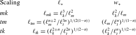
asymptote (see also table 2 for a summary of all different transition scales).
Characteristic scales in the different possible edge scalings – note that
 $p_{\ast }=E^{\prime }w_{\ast }/\ell _{\ast }$
and
 $Re_{\ast }=\unicode[STIX]{x1D70C}w_{\ast }V/\unicode[STIX]{x1D707}$
.

3.2 Turbulent asymptote
The previous laminar solution is valid up to the abscissa
 $\hat{x}_{t}$
where the Reynolds number
 $Re=\unicode[STIX]{x1D70C}wV/\unicode[STIX]{x1D707}$
reaches the critical value for the onset of turbulent flow. Another asymptote – that we shall denote as the turbulent asymptote (subscript
 $t$
) – can be obtained assuming that the turbulent flow is strictly in one of the limiting regimes previously discussed (Blasius, Gauckler–Manning–Strickler or maximum drag reduction case). The power-law-like lubrication relation (2.15) reads, in the moving tip coordinate system,
 $$\begin{eqnarray}\displaystyle V^{m}=\frac{w^{n+1}}{c}\frac{\text{d}p}{\text{d}\hat{x}}, & & \displaystyle\end{eqnarray}$$
such that the semi-infinite hydraulic fracture asymptote in the far field for large
 $\hat{x}$
/large
 $Re$
(where the effect of fracture toughness can be neglected) follows the zero toughness asymptote for a power-law fluid obtained by Desroches et al. (Reference Desroches, Detournay, Lenoach, Papanastasiou, Pearson, Thiercelin and Cheng1994), as pointed out by Tsai & Rice (Reference Tsai and Rice2010),
 $$\begin{eqnarray}\displaystyle w_{t}=\unicode[STIX]{x1D6FD}_{n}\ell _{t}^{n/(n+2)}\hat{x}^{2/(n+2)},\quad p_{t}=-\unicode[STIX]{x1D6FF}_{n}E^{\prime }\left(\frac{\ell _{t}}{\hat{x}}\right)^{n/(n+2)},\quad \ell _{t}=\left(\frac{cV^{m}}{E^{\prime }}\right)^{1/n}, & & \displaystyle\end{eqnarray}$$
with the prefactors (see Desroches et al. Reference Desroches, Detournay, Lenoach, Papanastasiou, Pearson, Thiercelin and Cheng1994)
 $$\begin{eqnarray}\displaystyle \unicode[STIX]{x1D6FD}_{n}=\left(2\frac{(n+1)^{2}}{n}\tan \left[-\frac{2\unicode[STIX]{x03C0}}{n+2}\right]\right)^{1/(n+2)},\quad \unicode[STIX]{x1D6FF}_{n}=\frac{\unicode[STIX]{x1D6FD}_{n}(n+2)}{2}\cot \left(\frac{2\unicode[STIX]{x03C0}}{n+2}\right).\qquad & & \displaystyle\end{eqnarray}$$
This asymptote is notably valid for any type of limiting flow regime: turbulent rough (Gauckler–Manning–Strickler), turbulent smooth (Blasius) as well as the case with friction reducers at maximum drag reduction). It is worthwhile noting that the turbulent exponent
 $m$
does not enter into the functional form of the width and net pressure asymptote (but in the length scale
 $\ell _{t}$
). Only the exponent
 $n$
appearing in the generalised lubrication relation (2.15) impacts this far-field asymptote.
3.3 Complete solution for
$f\propto Re^{-\unicode[STIX]{x1D6FD}}$
in the turbulent regime for slickwater

It is possible to solve the complete semi-infinite fracture problem numerically for a given evolution of the friction factor
 $f$
– see Dontsov (Reference Dontsov2016a
) for the case of water without friction reducers. Here, focusing chiefly on the case of a friction reducer at maximum drag reduction, a simple piecewise power-law expression for the friction factor above and below a critical Reynolds number approximation appears appropriate (see figure 2)
 $$\begin{eqnarray}\displaystyle f=\left\{\begin{array}{@{}ll@{}}\begin{array}{@{}l@{}}12/Re,\\ f_{o}^{\prime }Re^{-\unicode[STIX]{x1D6FD}},\end{array}\quad & \begin{array}{@{}l@{}}Re<Re_{c},\\ Re>Re_{c},\end{array}\end{array}\right. & & \displaystyle\end{eqnarray}$$
with
 $Re=\unicode[STIX]{x1D70C}wV/\unicode[STIX]{x1D707}$
and
 $Re_{c}$
is chosen to ensure continuity of friction:
 $Re_{c}=(12/f_{o}^{\prime })^{1/(1-\unicode[STIX]{x1D6FD})}$
, i.e.
 $Re_{c}\approx 1132$
for the maximum drag reduction approximation. It is clear that a similar approximation for the case without a friction reducer results in a gross approximation of the transition region, which plays a significant role as discussed in Dontsov (Reference Dontsov2016a
). The method and qualitative evolution however remain the same. Using the scaling for the toughness to viscous asymptote transition in the laminar case (Garagash et al.
Reference Garagash, Detournay and Adachi2011), we scale the coordinate, width and pressure as,
 $$\begin{eqnarray}\displaystyle \unicode[STIX]{x1D709}=\hat{x}/\ell _{mk},\quad \unicode[STIX]{x1D6FA}=w/w_{mk},\quad \unicode[STIX]{x1D6F1}=p/p_{mk}, & & \displaystyle\end{eqnarray}$$
using the characteristic scales corresponding to the laminar
 $mk$
transition previously mentioned (see also table 2)
 $$\begin{eqnarray}\displaystyle \ell _{mk}=\frac{K^{\prime 6}}{E^{\prime 4}V^{2}\unicode[STIX]{x1D707}^{\prime 2}},\quad w_{mk}=\frac{K^{\prime 4}}{E^{\prime 3}V\unicode[STIX]{x1D707}^{\prime }},\quad p_{mk}=\frac{E^{\prime 2}V\unicode[STIX]{x1D707}^{\prime }}{K^{\prime 2}}. & & \displaystyle\end{eqnarray}$$
The Reynolds number reduces to
 $$\begin{eqnarray}\displaystyle Re=\frac{\unicode[STIX]{x1D70C}wV}{\unicode[STIX]{x1D707}}=Re_{mk}\times \unicode[STIX]{x1D6FA},\quad Re_{mk}=12\frac{\unicode[STIX]{x1D70C}K^{\prime 4}}{E^{\prime 3}\unicode[STIX]{x1D707}^{\prime 2}}\left(=\frac{\unicode[STIX]{x1D70C}K^{\prime 4}}{12E^{\prime 3}\unicode[STIX]{x1D707}^{2}}\right). & & \displaystyle\end{eqnarray}$$
Here,
 $Re_{mk}$
is a characteristic Reynolds number which does not depend on the velocity of the fracture but solely on the fluid and solid material properties. The dependence on velocity lies in the transition length scale
 $\ell _{mk}$
. In such a scaling, elasticity, the fracture propagation condition and generalised lubrication flow read
 $$\begin{eqnarray}\displaystyle \hat{\unicode[STIX]{x1D6F1}}=\frac{1}{4\unicode[STIX]{x03C0}}\int _{0}^{\infty }\frac{\unicode[STIX]{x2202}\hat{\unicode[STIX]{x1D6FA}}(\unicode[STIX]{x1D702})}{\unicode[STIX]{x2202}\unicode[STIX]{x1D702}}\frac{\text{d}\unicode[STIX]{x1D702}}{\unicode[STIX]{x1D709}-\unicode[STIX]{x1D702}}, & & \displaystyle\end{eqnarray}$$
 $$\begin{eqnarray}\displaystyle \unicode[STIX]{x1D6FA}=\unicode[STIX]{x1D709}^{1/2},\quad \unicode[STIX]{x1D709}\ll 1, & & \displaystyle\end{eqnarray}$$
 $$\begin{eqnarray}\displaystyle 1=\frac{\hat{\unicode[STIX]{x1D6FA}}}{\tilde{f}(\hat{\unicode[STIX]{x1D6FA}})}\frac{\text{d}\hat{\unicode[STIX]{x1D6F1}}}{\text{d}\unicode[STIX]{x1D709}}, & & \displaystyle\end{eqnarray}$$
with
 $$\begin{eqnarray}\displaystyle \tilde{f}=1,\quad \hat{\unicode[STIX]{x1D6FA}}<Re_{c}/Re_{mk}, & & \displaystyle\end{eqnarray}$$
 $$\begin{eqnarray}\displaystyle \tilde{f}=\frac{f_{o}^{\prime }}{12}\times {Re_{mk}}^{1-n}\hat{\unicode[STIX]{x1D6FA}}^{1-n},\quad \hat{\unicode[STIX]{x1D6FA}}>Re_{c}/Re_{mk}. & & \displaystyle\end{eqnarray}$$
There is therefore a family of solutions parameterised by the dimensionless tip Reynolds number
 $Re_{mk}$
. We solve this system of nonlinear singular integro-differential equations numerically using a Gauss–Chebyshev quadrature mapping the interval
 $[0,\infty [$
to
 $[-1,1[$
and a simple finite difference approximation of the pressure gradient. The discretisation yields a nonlinear system of equations that can then be solved with standard root finding techniques. The method is strictly similar – pending the nonlinearity associated with
 $\tilde{f}(\hat{\unicode[STIX]{x1D6FA}})$
– to the one described in Moukhtari & Lecampion (Reference Moukhtari and Lecampion2018) and Viesca & Garagash (Reference Viesca and Garagash2018) and will not be repeated here.
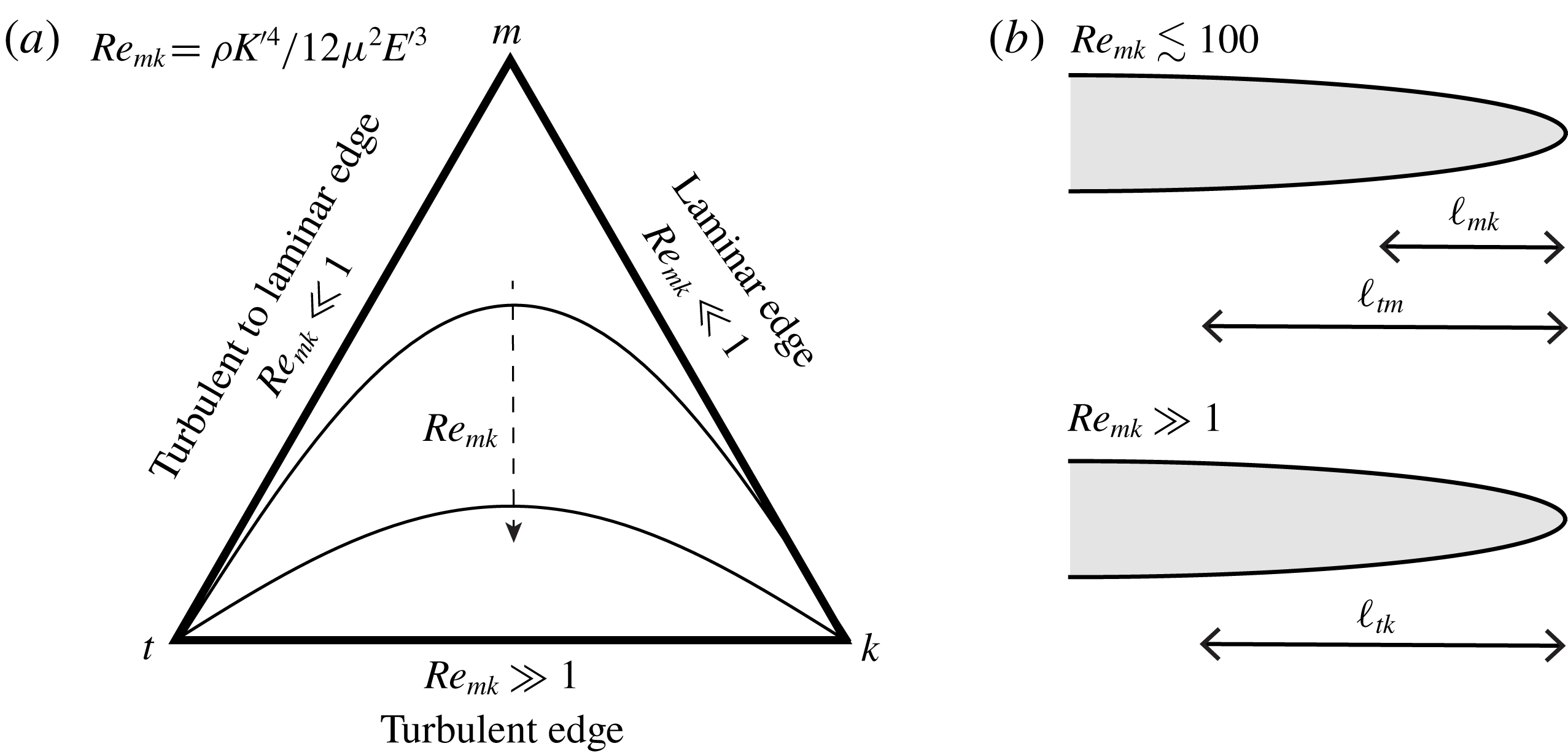
(a) Parametric diagram of the near-tip hydraulic fracture solution structure accounting for the transition to a turbulent flow regime (
 $f\propto Re^{-n}$
) with a few trajectories for different values of the tip Reynolds number
 $Re_{mk}$
; (b) structure of the solution for small and large values of
 $Re_{mk}$
. For order
 $Re_{mk}\lesssim 100$
, the viscous laminar asymptote (
 $m$
) is clearly visible in between the far-field turbulent (
 $t$
) and near-tip linear elastic fracture mechanics asymptote (
 $k$
). For large
 $Re_{mk}$
, the laminar viscous asymptote disappears altogether: the solution transitions directly from
 $t$
to
 $k$
as one moves closer to the tip.

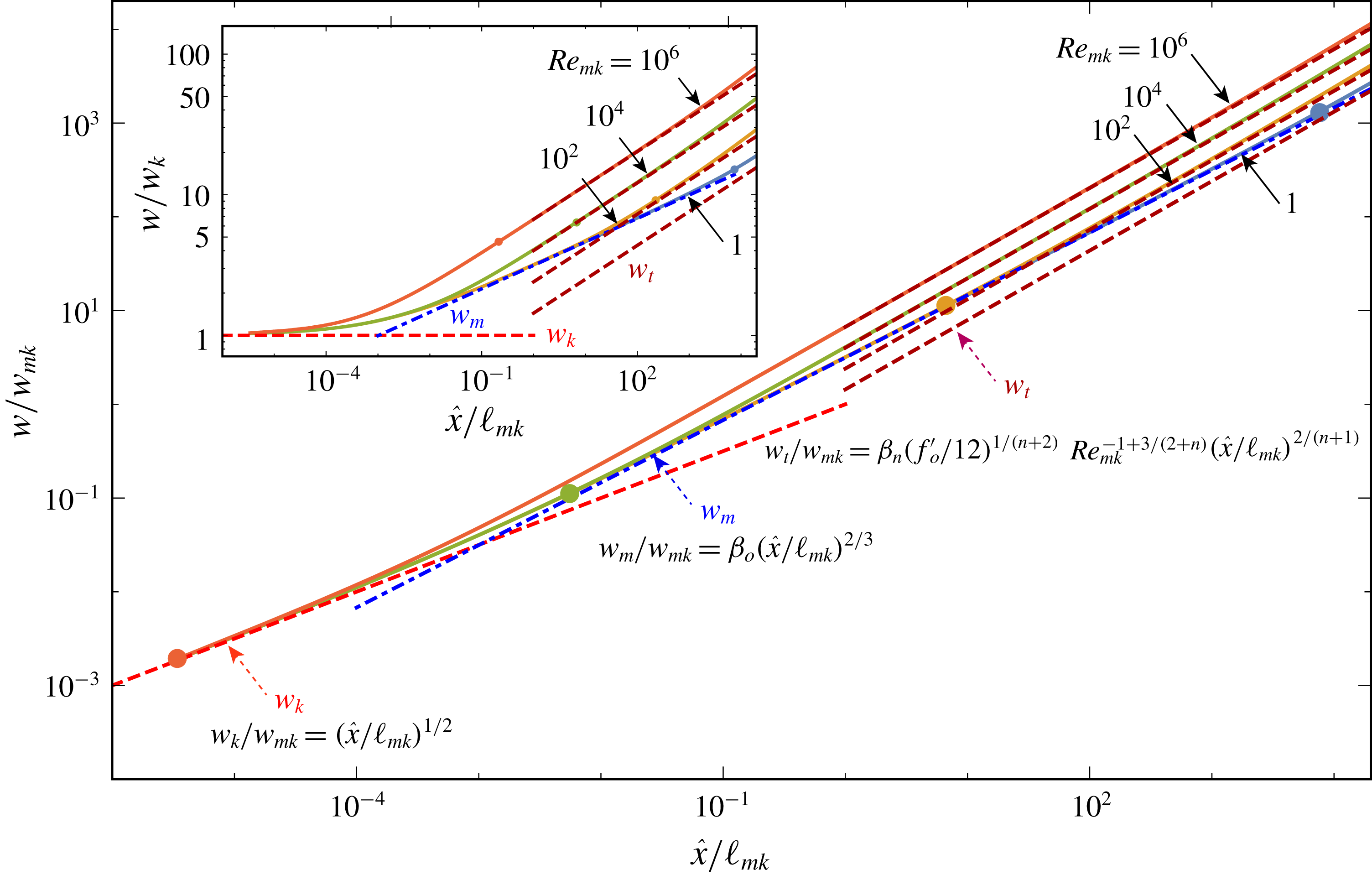
Figure 4 displays the results for different values of the tip Reynolds number
 $Re_{mk}$
. For small values of
 $Re_{mk}$
, the solution evolves from the toughness (
 $k$
) to the laminar viscous (
 $m$
) and ultimately the turbulent flow (
 $t$
) asymptotes as one moves away from the fracture tip. On the other hand, for large
 $Re_{mk}$
(above
 $10^{5}$
), the viscous laminar region disappears and the solution transitions directly from the toughness (
 $k$
) to the turbulent (
 $t$
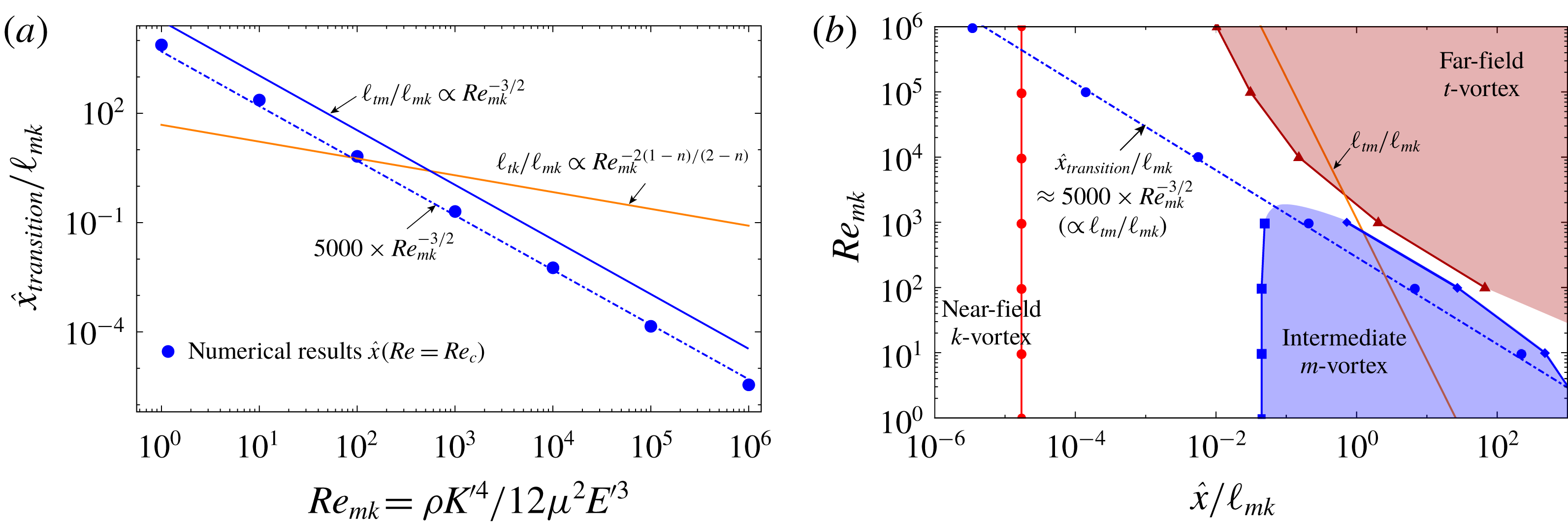
) flow asymptote, with the toughness region also shrinking. This is in line with the fact that for very large Reynolds numbers, the laminar region shrinks, as figure 3 shows. The transition length scale between the different limiting asymptotes can be obtained from arguments similar to the solely laminar case (i.e. equalising the width scales of the two different asymptotes to obtain the transition scale), thus defining different edge scalings (see table 2). From these transition length scales, and our numerical results, it is possible to estimate the distance from the tip
 $\hat{x}_{transition}$
where the flow transitions from laminar to turbulent: intuitively
 $\hat{x}_{transition}$
should scale with the length scale
 $\ell _{tm}$
governing the transition between the turbulent and laminar asymptotic regions. This is indeed the case, as can be seen in figure 5(a), where the location at which the local Reynolds number equals the critical value obtained from our numerical results, is compared with the transition length scale
 $\ell _{tm}$
as a function of the tip characteristic Reynolds number
 $Re_{mk}$
. One sees from figure 5(a) that the extent of the laminar layer is well approximated as
 $$\begin{eqnarray}\displaystyle \hat{x}_{transition}\approx 5000Re_{mk}^{-3/2}\ell _{mk}. & & \displaystyle\end{eqnarray}$$
From figure 5, we also observe that for values of
 $Re_{mk}$
greater than
 ${\sim}10^{3}$
, the turbulent to viscous laminar transition scale
 $\ell _{tm}$
becomes smaller than the turbulent to toughness transition scale
 $\ell _{tk}$
such that the laminar viscous asymptote (
 $m$
) disappears, as observed in the solution for width (figure 4). The domain of validity of the different tip asymptotes can also be well grasped from figure 5(b). It can be well observed that the laminar viscous asymptote disappears for
 $Re_{mk}>10^{3}$
while in the meantime the turbulent asymptotic region moves closer to the tip (and its location scales with
 $\ell _{tk}$
for large
 $Re_{mk}$
). The fact that the extent of the laminar layer (
 $\hat{x}_{transition}$
) scales with
 $\ell _{tm}$
even for large Reynolds numbers is due to the fact that, even though the laminar viscous asymptote is not fully realised, laminar flow still influences the solution in the intermediate region. The transition from the turbulent to the toughness asymptote scales qualitatively with
 $\ell _{tk}$
for large
 $Re_{mk}$
. However
 $\ell _{tk}$
does not physically include the effect of laminar flow (and thus is not the proper scale for the laminar region).
Near-tip solution for a slickwater hydraulic fracture accounting for turbulent flow at maximum drag reduction: numerical results (continuous lines) and
 $t$
,
 $m$
and
 $k$
asymptotes. Width as a function of tip distance (in the
 $mk$
scaling) for different values of the tip Reynolds number (inset: same results but scaled by the toughness near-tip asymptote
 $w_{k}$
). The dots correspond to the boundary of the laminar flow region near the tip.

(a) Evolution of the laminar region in the near-tip region as function of the tip Reynolds number. The laminar–turbulent transition distance
 $\hat{x}_{transition}$
is obtained from the numerical results as the distance (up to the discretisation) where
 $Re=Re_{c}$
(bullet points). The transition length scale
 $\ell _{tm}$
provides a qualitative estimate of the laminar region (continuous blue line), while a better approximation (with the same dependence on
 $Re_{mk}$
) as the numerical results is obtained at
 $5000\times Re_{mk}^{-3/2}$
(dashed-dotted line). (b) Domains of validity of the different asymptotes (
 $m,k,t$
) as a function of normalised distance from the tip
 $\hat{x}/\ell _{mk}$
and
 $Re_{mk}$
. The boundaries of the domains correspond to the locations where the numerical solution is within a
 $5\,\%$
relative difference from the corresponding tip asymptote. The laminar–turbulent transition distance
 $\hat{x}_{transition}/\ell _{mk}$
is also plotted.

Such a simple estimation of the extent of the laminar layer (3.19) as well as the disappearance of the viscous asymptote for
 $Re_{mk}\gtrsim 10^{3}$
are extremely useful in practice to quickly determine the importance of taking into account the turbulent flow behaviour in a numerical simulation of hydraulic fracture growth. It is also worthwhile noting that the entire solution for the
 $tm$
and
 $tk$
edges of this near-tip solution can be very well approximated (up to 1.5 % of maximum relative error) by a simple first-order approximation similar to the one proposed for the laminar
 $mk$
edge by Dontsov & Peirce (Reference Dontsov and Peirce2015). These approximations are listed in appendix B for convenience.
This semi-infinite hydraulic fracture solution provides the near-tip width asymptote of the radial hydraulic fracture by replacing
 $V$
with the current radial fracture velocity
 $\text{d}R/\text{d}t$
(see discussions in Detournay & Peirce (Reference Detournay and Peirce2014), Dontsov & Kresse (Reference Dontsov and Kresse2018) and Lecampion, Bunger & Zhang (Reference Lecampion, Bunger and Zhang2018)).
4 Scalings and structure of the solution for a radial hydraulic fracture
We now return to the propagation of a finite radial hydraulic fracture. Similarly as for the laminar case (Savitski & Detournay Reference Savitski and Detournay2002), we introduce the following scalings for fracture width, net pressure, fracture radius and fluid velocity:
 $$\begin{eqnarray}\displaystyle w(r,t)=\underbrace{\unicode[STIX]{x1D716}(t)L(t)}_{W(t)}\unicode[STIX]{x1D6FA}(\unicode[STIX]{x1D709}),\quad p(r,t)=\unicode[STIX]{x1D716}(t)E^{\prime }\unicode[STIX]{x1D6F1}(\unicode[STIX]{x1D709}),\quad R(t)=L(t)\unicode[STIX]{x1D6FE},\quad v(r,t)=\frac{L(t)}{t}{\mathcal{V}}(\unicode[STIX]{x1D709}), & & \displaystyle \nonumber\\ \displaystyle & & \displaystyle\end{eqnarray}$$
where
 $\unicode[STIX]{x1D716}$
is a small dimensionless number and
 $L$
a characteristic length – both of which are functions of time;
 $\unicode[STIX]{x1D6FE}$
,
 $\unicode[STIX]{x1D6FA}$
,
 $\unicode[STIX]{x1D6F1}$
and
 ${\mathcal{V}}$
denote the dimensionless fracture radius, fracture width, net pressure and fluid velocity that may be a function of a set of dimensionless parameters. We also scale the radial coordinates by the current fracture radius
 $R(t)$
,
 $\unicode[STIX]{x1D709}=r/R(t)$
. The previous scaling recognises the fact that the fracture width is typically much smaller than its length (
 $w/R\propto \unicode[STIX]{x1D716}$
) and that it is of the same order as the ratio between the net pressure loading (fluid pressure minus the normal in situ stress to the fracture plane) and the plane-strain elastic modulus (see Detournay Reference Detournay2004, Reference Detournay2016). In such a scaling and system of coordinates, the set of governing equations (2.1)–(2.11) now takes the following form:
(i) Elasticity (2.1)
(4.2)$$\begin{eqnarray}\displaystyle \unicode[STIX]{x1D6FA}(\unicode[STIX]{x1D709})=\frac{8\unicode[STIX]{x1D6FE}}{\unicode[STIX]{x03C0}}\int _{0}^{1}G(\unicode[STIX]{x1D709},\unicode[STIX]{x1D709}^{\prime })\unicode[STIX]{x1D6F1}(\unicode[STIX]{x1D709}^{\prime })\unicode[STIX]{x1D709}^{\prime }\,\text{d}\unicode[STIX]{x1D709}^{\prime }. & & \displaystyle\end{eqnarray}$$
(ii) Fracture propagation condition in terms of the Bueckner–Rice integral (2.2)
(4.3)where$$\begin{eqnarray}\displaystyle \underbrace{\frac{K^{\prime }}{\unicode[STIX]{x1D716}E^{\prime }L^{1/2}}}_{{\mathcal{G}}_{k}}\frac{\unicode[STIX]{x03C0}}{2^{7/2}}=\unicode[STIX]{x1D6FE}^{1/2}\int _{0}^{1}\frac{\unicode[STIX]{x1D6F1}(\unicode[STIX]{x1D709})}{\sqrt{1-\unicode[STIX]{x1D709}^{2}}}\unicode[STIX]{x1D709}\,\text{d}\unicode[STIX]{x1D709}, & & \displaystyle\end{eqnarray}$$
${\mathcal{G}}_{k}$
is akin to a dimensionless fracture toughness, and
$K^{\prime }=\sqrt{32/\unicode[STIX]{x03C0}}K_{Ic}$
as defined for clarity in Detournay (Reference Detournay2004).(iii) The fluid continuity equation (2.3) in this moving system of coordinates reads
(4.4)where a dot means a time derivative.$$\begin{eqnarray}\displaystyle \dot{\unicode[STIX]{x1D6FA}}+\left(\frac{\dot{\unicode[STIX]{x1D716}}}{\unicode[STIX]{x1D716}}t+\frac{\dot{L}}{L}t\right)\unicode[STIX]{x1D6FA}-\left(\frac{\dot{L}}{L}t+\frac{\dot{\unicode[STIX]{x1D6FE}}}{\unicode[STIX]{x1D6FE}}t\right)\unicode[STIX]{x1D709}\frac{\unicode[STIX]{x2202}\unicode[STIX]{x1D6FA}}{\unicode[STIX]{x2202}\unicode[STIX]{x1D709}}+\frac{1}{\unicode[STIX]{x1D6FE}}\frac{1}{\unicode[STIX]{x1D709}}\frac{\unicode[STIX]{x2202}}{\unicode[STIX]{x2202}\unicode[STIX]{x1D709}}\unicode[STIX]{x1D709}\unicode[STIX]{x1D6FA}{\mathcal{V}}=0, & & \displaystyle\end{eqnarray}$$
(iv) The generalised lubrication relation (2.15)
(4.5)where$$\begin{eqnarray}\displaystyle {\mathcal{V}}^{m}=-\underbrace{\frac{t^{m}\unicode[STIX]{x1D716}^{n+2}E^{\prime }}{L^{m-n}c}}_{{\mathcal{G}}_{f}^{-1}}\frac{\unicode[STIX]{x1D6FA}^{n+1}}{\unicode[STIX]{x1D6FE}}\frac{\unicode[STIX]{x2202}\unicode[STIX]{x1D6F1}}{\unicode[STIX]{x2202}\unicode[STIX]{x1D709}}, & & \displaystyle\end{eqnarray}$$
${\mathcal{G}}_{f}$
is akin to a dimensionless friction/viscosity.(v) The inlet boundary condition (2.4)
(4.6)$$\begin{eqnarray}\displaystyle \lim _{\unicode[STIX]{x1D709}\rightarrow 0}2\unicode[STIX]{x03C0}\unicode[STIX]{x1D6FE}\unicode[STIX]{x1D709}\unicode[STIX]{x1D6FA}{\mathcal{V}}=\underbrace{\frac{Q_{o}t}{\unicode[STIX]{x1D716}L^{3}}}_{{\mathcal{G}}_{q}}. & & \displaystyle\end{eqnarray}$$
(vi) The tip boundary conditions (2.5)
(4.7a,b )$$\begin{eqnarray}\displaystyle \unicode[STIX]{x1D6FA}(1)=0,\quad \unicode[STIX]{x1D6FA}(1){\mathcal{V}}(1)=0. & & \displaystyle\end{eqnarray}$$


We have implicitly focused above on the case where a single limiting flow regime was valid over the whole fracture length, and used the generalised version of the lubrication (2.15) over the whole fracture length. In order to grasp the evolution of the propagation of hydraulic fractures and the transition between limiting flow regimes, it is important to keep in mind that friction (which governs the pressure – velocity relation) is a function of both the Reynolds number (2.10) and the relative roughness
 $k_{R}/w$
. The Reynolds number (2.10), which is spatially varying along the fracture, can be rewritten as
 $$\begin{eqnarray}\displaystyle Re_{D_{eq}}={\textstyle \frac{4}{3}}{\mathcal{R}}\,\unicode[STIX]{x1D6FA}\,{\mathcal{V}}, & & \displaystyle\end{eqnarray}$$
where
 ${\mathcal{R}}$
is the characteristic Reynolds number
 $$\begin{eqnarray}\displaystyle {\mathcal{R}}=\frac{\unicode[STIX]{x1D70C}\unicode[STIX]{x1D716}L^{2}}{\unicode[STIX]{x1D707}\times t}=\frac{\unicode[STIX]{x1D70C}Q_{o}}{\unicode[STIX]{x1D707}L(t)} & & \displaystyle\end{eqnarray}$$
while the relative roughness is simply given as
 $$\begin{eqnarray}\displaystyle k_{R}/w=\frac{k_{R}}{\unicode[STIX]{x1D716}L}\frac{1}{\unicode[STIX]{x1D6FA}}. & & \displaystyle\end{eqnarray}$$
We see that the Reynolds number will be large at early times, and will decay as the fracture radius
 $L(t)$
increases with time. Similarly, relative roughness will dominate at early time/small fracture size. Turbulent flow regimes will therefore dominate for large
 ${\mathcal{R}}$
/small times, and the flow will necessarily transition toward laminar flow at large times. Moreover, we also note that
 $Re_{D_{eq}}$
necessarily goes to zero at the fracture tip due to the boundary conditions (4.7), while relative roughness, of course, dominates at the fracture tip, if the flow is turbulent. As previously discussed in regards to the near-tip solution, a laminar region always exists at the fracture tip, but such a region shrinks as a boundary layer for large Reynolds number (see figure 5).
Under the assumption of a single limiting flow regime over the whole fracture, only three dimensionless groups
 $({\mathcal{G}}_{q},{\mathcal{G}}_{k},{\mathcal{G}}_{m})$
directly appear in the previous system of equations, two of which must be set to unity in order to define the characteristic length scale
 $L$
and fracture width scale
 $W=\unicode[STIX]{x1D716}L$
. We set
 ${\mathcal{G}}_{q}=1$
in the case of an impermeable material, as the injected volume remains always equal to the fracture volume (Detournay Reference Detournay2004), and thus obtain the following expression for
 $\unicode[STIX]{x1D716}$
:
 $$\begin{eqnarray}\displaystyle \unicode[STIX]{x1D716}=\frac{Q_{o}t}{L^{3}}. & & \displaystyle\end{eqnarray}$$
The two remaining dimensionless numbers, namely the dimensionless toughness
 ${\mathcal{G}}_{k}$
and friction/viscosity
 ${\mathcal{G}}_{f}$
can now be expressed as function of a yet unknown characteristic length scale
 $L(t)$
and the problem parameters,
 $$\begin{eqnarray}\displaystyle {\mathcal{G}}_{k}=\frac{K^{\prime }L^{5/2}}{E^{\prime }Q_{o}t},\quad {\mathcal{G}}_{f}=\frac{c\,L^{6+2n+m}}{E^{\prime }Q_{o}^{n+2}t^{2+m+n}}. & & \displaystyle\end{eqnarray}$$
As in the laminar case Savitski & Detournay (Reference Savitski and Detournay2002), two type of scalings can thus be devised depending on which dissipative process dominates: in the creation of new fracture surfaces or in fluid flow.
4.1 Friction/viscous scalings
In the case where the energy dissipated in lubrication flow is larger than the energy spent in the creation of new surfaces, the dominance of the fluid friction dictates setting
 ${\mathcal{G}}_{f}$
to unity. We thus obtain the following estimate of the characteristic fracture length scale
 $L$
for the universal lubrication relation (2.15):
 $$\begin{eqnarray}\displaystyle L_{f}=\left(\frac{E^{\prime }Q_{o}^{n+2}t^{m+n+2}}{c}\right)^{1/(6+m+2n)}, & & \displaystyle\end{eqnarray}$$
where the subscript
 $f$
refers to such a fluid friction/viscous scaling. The dimensionless group
 ${\mathcal{G}}_{k}$
associated with fracture energy can be re-expressed in that scaling as a dimensionless toughness
 $$\begin{eqnarray}\displaystyle {\mathcal{K}}=K^{\prime }\times \left(\frac{t}{E^{\prime ^{(7+2m+4n)/(3m+n-2)}}Q_{o}^{5m/(3m+n-2)-1}c^{5/(3m+n-2)}}\right)^{(3m+n-2)/(2(6+m+2n))}, & & \displaystyle\end{eqnarray}$$
while the characteristic Reynolds number (4.9) in such a scaling is
 $$\begin{eqnarray}\displaystyle {\mathcal{R}}=\frac{\unicode[STIX]{x1D70C}Q_{o}}{\unicode[STIX]{x1D707}L_{f}}=\left(\frac{\unicode[STIX]{x1D70C}}{\unicode[STIX]{x1D707}}\frac{Q_{o}^{(4+m+n)/(2+m+n)}}{t}\left(\frac{c}{E^{\prime }}\right)^{1/(2+m+n)}\right)^{(2+m+n)/(6+m+2n)}. & & \displaystyle\end{eqnarray}$$
It is worthwhile noting that the dimensionless toughness increases with time. It can be expressed via the introduction of a characteristic time scale
 $t_{f\rightarrow k}$
 $$\begin{eqnarray}\displaystyle {\mathcal{K}}=\left(\frac{t}{t_{f\rightarrow k}}\right)^{3m+n-2/(2(6+m+2n))},\quad t_{f\rightarrow k}=\frac{E^{\prime (7+2m+4n)/(3m+n-2)}c^{5/(3m+n-2)}Q_{o}^{(2m+2-n)/(3m+n-2)}}{K^{\prime (2(6+m+2n))/(3m+n-2)}}.\hspace{-5.0pt} & & \displaystyle \nonumber\\ \displaystyle & & \displaystyle\end{eqnarray}$$
Similarly, the characteristic Reynolds number decreases with time, indicating that turbulent flow dominates at early times, and becomes negligible when
 ${\mathcal{R}}<{\mathcal{R}}_{c}$
. This allows us to define a transition time scale for the transition towards the laminar regime
 $t_{t\rightarrow l}$
, such that the characteristic Reynolds number can be written as
 $$\begin{eqnarray}\displaystyle {\mathcal{R}}={\mathcal{R}}_{c}\left(\frac{t}{t_{t\rightarrow l}}\right)^{-((2+m+n)/(6+m+2n))},\quad t_{t\rightarrow l}=\frac{c^{1/(2+m+n)}Q_{o}^{1+(2/(2+m+n))}\unicode[STIX]{x1D70C}^{(6+m+2n)/(2+m+n)}}{E^{\prime 1/(2+m+n)}\unicode[STIX]{x1D707}^{2+(2-m/2+m+n)}{\mathcal{R}}_{c}^{2+(2-m/(2+m+n))}}. & & \displaystyle \nonumber\\ \displaystyle & & \displaystyle\end{eqnarray}$$
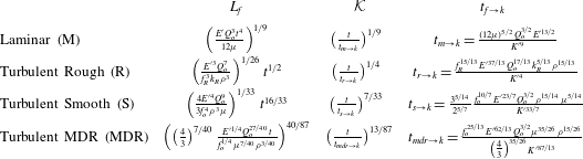
Characteristic length scale
 $L_{f}$
and dimensionless toughness in the different fluid friction dominated scalings. The corresponding width scales as
 $W=\unicode[STIX]{x1D716}L_{f}=Q_{o}t/L_{f}^{2}$
, while the characteristic pressure is
 $P=E^{\prime }Q_{o}t/L_{f}^{3}$
. Note that the complete friction factor depends in the general case on both Reynolds number and relative roughness. The Reynolds number scales with the characteristic value
 ${\mathcal{R}}=\unicode[STIX]{x1D70C}Q_{o}/(\unicode[STIX]{x1D707}\,L_{f}(t))$
, while the relative roughness scales as
 $k_{R}/W$
. For the turbulent smooth and MDR regimes the corresponding expressions for
 $f_{o}$
are listed in (2.13) and (2.14) respectively.

Such a friction scaling is valid for the different flow regimes (different
 $m,n$
and
 $c$
) where the lubrication velocity–pressure gradient relation can be expressed in the general form (2.15). The exact expressions for the turbulent rough, turbulent smooth as well as the maximum drag reduction regimes can be found in table 3. We obviously recover the viscosity scaling in the laminar case. It is interesting to note that the power laws of time for the characteristic length are
 $1/2$
,
 $16/33$
and
 $40/87$
respectively for the rough, smooth and MDR regimes – all very close to
 $1/2$
. As a result, the fracture width, which scales as
 $W=Q_{o}t/L_{f}^{2}$
, will either be constant (rough regimes) or evolves slowly as
 $t^{1/33}$
and
 $t^{7/87}$
.
It is important to keep in mind that these scalings are based on the underlying assumption that the flow regime is the same over the whole fracture length. Changes in the flow regimes will occur within the fracture in relation to the local value of the Reynolds number which depends on the characteristic Reynolds number
 ${\mathcal{R}}$
which scales as
 $1/L_{f}$
, as well as the local dimensionless fracture width and velocity (see (4.8)). Therefore, a transition between flow regimes will necessarily occur within the growing fracture as time progresses and a laminar region, albeit small, always exist near the fracture tip. Nevertheless, at early times, one can build a limiting self-similar solution for the growth of a radial hydraulic fracture for each of the flow regimes: laminar, rough turbulent, smooth turbulent or at maximum drag reduction (in the case with friction reducing additives).
4.2 Toughness scaling
The other limiting scaling corresponds to the case where most of the energy is dissipated in the solid, creating new fracture surfaces. Setting
 ${\mathcal{G}}_{k}=1$
, one recovers the well-known toughness dominated scaling (Savitski & Detournay Reference Savitski and Detournay2002), where the characteristic length scale is independent of the fluid properties
 $$\begin{eqnarray}\displaystyle L_{k}=\left(\frac{E^{\prime }Q_{o}t}{K^{\prime }}\right)^{2/5} & & \displaystyle\end{eqnarray}$$
and the corresponding dimensionless ‘viscosity’
 ${\mathcal{G}}_{f}$
becomes
 $$\begin{eqnarray}\displaystyle {\mathcal{M}}=c\times \left(\frac{Q_{o}^{(2+2m-n)/(3m+n-2)}E^{\prime (7+2m+4n)/(3m+n-2)}}{K^{\prime ((2(6+m+2n))/(2m+n-2))}t}\right)^{5/(3m+n-2)}. & & \displaystyle\end{eqnarray}$$
There is of course a correspondence with the friction/lubrication scalings
 $$\begin{eqnarray}\displaystyle {\mathcal{K}}={\mathcal{M}}^{-5/(2(6+m+2n))},\quad \frac{L_{k}}{L_{f}}={\mathcal{K}}^{-2/5}. & & \displaystyle\end{eqnarray}$$
4.3 Structure of the solution
In the case of solely laminar flow, the hydraulic fracture growth solution evolves from the viscosity dominated regime of propagation at small times to the toughness dominated regime at large times (Savitski & Detournay Reference Savitski and Detournay2002). The time scale of this transition
 $t_{m\rightarrow k}$
is the one appearing in the expression for the dimensionless toughness
 ${\mathcal{K}}$
(see table 3). Such a transition can be physically grasped as the energy spent in creating new surfaces increases as
 $2\unicode[STIX]{x03C0}R\,\text{d}R$
for such an axisymmetric fracture and thus necessarily dominates at large times. In the laminar case, it was shown that the viscosity dominated regime is valid up to
 ${\mathcal{K}}=1$
while the toughness dominated regime starts for dimensionless toughness larger than
 $3.5$
(Savitski & Detournay Reference Savitski and Detournay2002).
When accounting for turbulent regimes, the solution structure is similar at large times, as here again the dimensionless toughness
 ${\mathcal{K}}$
increases with time as
 $\propto t^{\unicode[STIX]{x1D6FC}}$
(with
 $\unicode[STIX]{x1D6FC}>0$
), as can be seen in table 3 for all the different limiting flow regimes. However, other time scales appear associated with the transition between the different flow regimes as functions of the Reynolds number and characteristic roughness. We first discuss the case of plain water without friction reducing additives, where both rough and smooth turbulent regimes can occur.
4.3.1 Water (without friction reducers)
As discussed previously, the characteristic Reynolds number evolves as
 $1/L$
(4.9), such that turbulent regimes will dominate at the early times of fracture growth. Moreover, at early times, fracture roughness is bound to dominate as the fracture width will be small and comparable to the roughness scale. The following picture therefore emerges for the case of plain water without friction reducers. At early times, the propagation will be dominated by the rough turbulent regime. As time progresses, one may transition to the turbulent smooth regime as the fracture widens compared to the roughness scales, then to the laminar viscous dominated regime and ultimately to the toughness dominated regime. However, it may well be possible that the HF growth directly transitions from the turbulent rough to the toughness dominated regime. In order to grasp the transition between the different flow regimes, one can easily determine the time at which the characteristic fracture scale
 $L_{f}$
is equal for both limiting regimes. In doing so, one can define three time scales corresponding respectively to (i) the transition between the rough and smooth turbulent regimes (
 $t_{r\rightarrow s}$
), (ii) the turbulent rough and laminar regimes (
 $t_{r\rightarrow m}$
) and (iii) the turbulent smooth and laminar regimes (
 $t_{s\rightarrow m}$
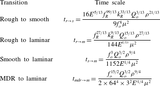
). All these time scales are listed in table 4. The transition time scales from the turbulent to the laminar regime could also have been obtained by arguing that the laminar regime is reached when the characteristic Reynolds number
 ${\mathcal{R}}$
falls below the critical laminar–turbulent transition value
 ${\mathcal{R}}_{c}$
(similar results are obtained up to a constant factor).
Transition time scales between regimes of propagation governed by the different limiting flow regimes.

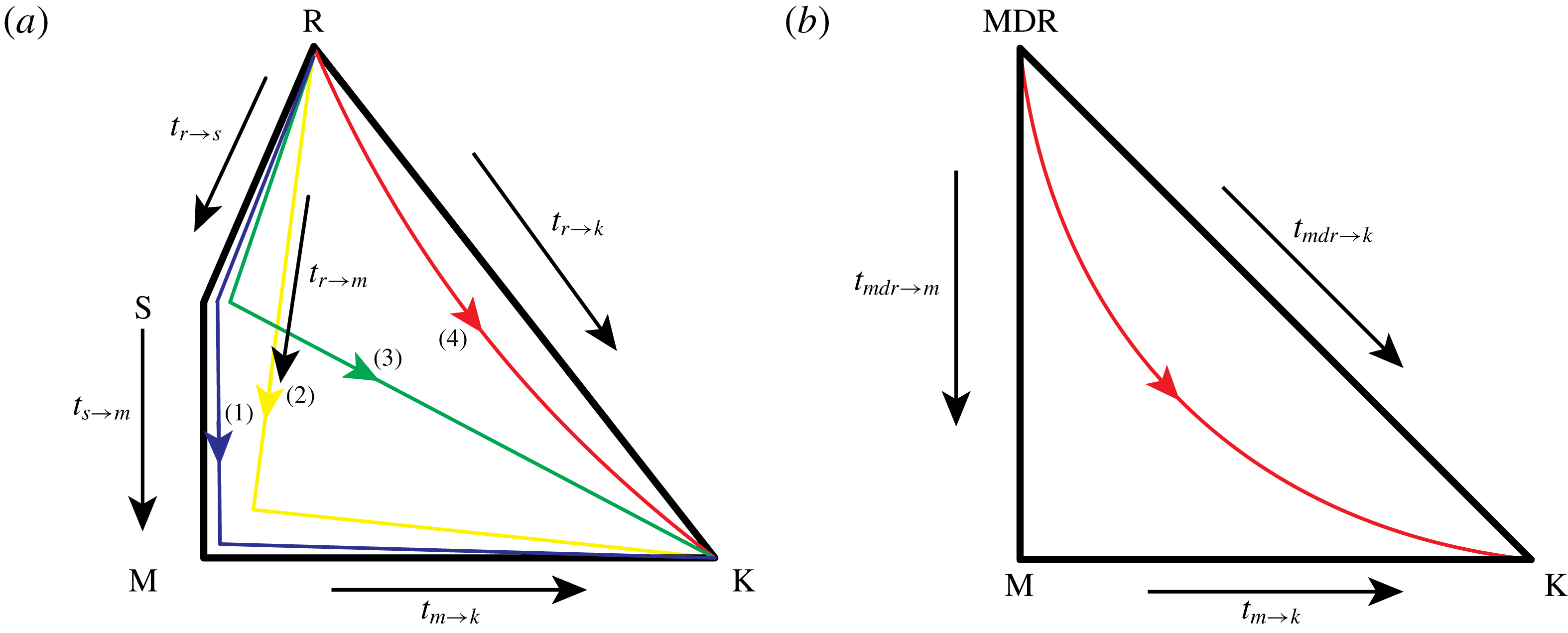
As a result, four different situations may be encountered during the growth of a radial fracture, as depicted in figure 6, depending on the relative value of the transition time scales between flow regimes as well as the transition time scales from a given flow regime to the toughness dominated regime (table 3).
Propagation diagram for a radial hydraulic fracture: water without friction reducers (a) and slickwater with friction reducer at maximum drag reduction (b).

For the sake of illustration, let us consider the following values of the parameters (corresponding to water injected at a very high rate in an ‘average’ sedimentary rock):
 $$\begin{eqnarray}\displaystyle E^{\prime }=20~\text{GPa},\quad Q_{o}=0.079~\text{m}^{3}~\text{s}^{-1},\quad \unicode[STIX]{x1D70C}=1000~\text{kg}~\text{m}^{-3}, & & \displaystyle\end{eqnarray}$$
 $$\begin{eqnarray}\displaystyle \unicode[STIX]{x1D707}=1~\text{cP},\quad K_{Ic}=0.5~\text{MPa}\,\sqrt{\text{m}},\quad k_{R}=500~\unicode[STIX]{x03BC}\text{m}, & & \displaystyle\end{eqnarray}$$
for which we obtain the following transition time scales between the different limiting regimes (all times in seconds):
 $$\begin{eqnarray}\displaystyle \left.\begin{array}{@{}l@{}}t_{r\rightarrow s}=97\,681,\quad t_{r\rightarrow m}=844,\quad t_{s\rightarrow m}=142,\\ t_{r\rightarrow k}=5049,\quad t_{s\rightarrow k}=2975,\quad t_{m\rightarrow k}=47\,245.\end{array}\right\} & & \displaystyle\end{eqnarray}$$
For that particular set of parameters, the propagation will evolve from the roughness turbulent dominated regime, toward the laminar viscous dominated regime to ultimately the toughness dominate regime at large times: along trajectory (2) in figure 6. The smooth turbulent regime will not appear as
 $t_{r\rightarrow s}\gg t_{r\rightarrow m}$
. Moreover the transition to the laminar viscous dominated regime occurs faster than the transition from the rough to the toughness dominated regime
 $t_{r\rightarrow m}\ll t_{r\rightarrow k}$
.
Note that other types of trajectories are possible as functions of the problem parameters. For a larger toughness, a transition directly from the rough turbulent to the toughness regime can occur (trajectory (4) in figure 6), or for a smaller value of the roughness scale
 $k_{R}$
, the smooth turbulent regimes may appear (trajectories (1) and (3) in figure 6). The diagram and limiting trajectories depicted in figure 6 in combination with the different transition time scales allows us to directly quantify the regimes encountered during the growth of a radial hydraulic fracture without doing any numerical simulations.
4.3.2 Slickwater (water with friction reducers)
In the case where friction reducing agents are added in sufficient concentration to water, the turbulent flow is governed by the drag reduction asymptote and roughness appears to have little effect here for Reynolds numbers lower than
 $3\times 10^{4}$
(see figure 2). From the expected ranges of Reynolds number in applications (always lower than
 $10^{5}$
), the situation is therefore simpler than for the previously discussed water case. Beside the transition towards the toughness dominated regime at large times, there exists here only one additional time scale governing the transition from the turbulent/MDR regime toward the laminar viscous dominated one. Similarly, the expression for such a time scale
 $t_{mdr\rightarrow m}$
can be easily obtained by solving for the time at which the characteristic fracture scales in the MDR and laminar regimes are equal – see table 4.
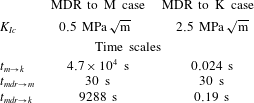
The diagram picturing the possible trajectory from one regime to the next for a radial HF growing with friction reducing additives is depicted in figure 6(b). For the same set of parameters used previously, we obtain in the slickwater case the following transition time scales (time in seconds)
 $$\begin{eqnarray}\displaystyle t_{mdr\rightarrow m}=83,\quad t_{mdr\rightarrow k}=9288,\quad t_{m\rightarrow k}=47\,245. & & \displaystyle\end{eqnarray}$$
For that particular case, the HF quickly transitions to the viscous laminar dominated regime (
 $t_{mdr\rightarrow m}\ll t_{mdr\rightarrow k}$
) and then moves toward the toughness dominated regime at large times. For a larger value of fracture toughness (2.5 instead of 0.5), we obtain the opposite case
 $t_{mdr\rightarrow m}(=30~\text{s})>t_{mdr\rightarrow k}(=30~\text{s})$
such that the HF will move directly from the MDR dominated to the toughness dominated regime.
5 Zero toughness propagation solutions for radial fractures
We now derive semi-analytical solutions for the zero toughness case, assuming that a limiting flow regime (rough, smooth MDR etc.) applies over the whole fracture. Such a family of solutions is valid at early times in the propagation of a turbulent hydraulic fracture when the fracture energy is negligible compared to fluid friction losses.
We follow here the solution procedure devised originally by Savitski & Detournay (Reference Savitski and Detournay2002) for the viscous laminar case. We slightly adapt it to the generalised lubrication equation (2.15). As discussed previously, for the early time/zero toughness case, the dimensionless solution does not depend on any dimensionless parameters – pending the hypothesis of a fully turbulent flow model (rough, smooth, smooth with friction reducer etc.). The solution is therefore self-similar. All the time dependence is encapsulated in the characteristic scales (table 3). Following Savitski & Detournay (Reference Savitski and Detournay2002), we solve for a reduced dimensionless opening – defined as
 $$\begin{eqnarray}\displaystyle \bar{\unicode[STIX]{x1D6FA}}(\unicode[STIX]{x1D709})=\unicode[STIX]{x1D6FA}(\unicode[STIX]{x1D709})/\unicode[STIX]{x1D6FE}, & & \displaystyle\end{eqnarray}$$
which is directly related to the dimensionless net pressure via the dimensionless elasticity equation
 $$\begin{eqnarray}\displaystyle \bar{\unicode[STIX]{x1D6FA}}(\unicode[STIX]{x1D709})=\frac{8}{\unicode[STIX]{x03C0}}\int _{0}^{1}G(\unicode[STIX]{x1D709},\unicode[STIX]{x1D709}^{\prime })\unicode[STIX]{x1D6F1}(\unicode[STIX]{x1D709}^{\prime })\unicode[STIX]{x1D709}^{\prime }\,\text{d}\unicode[STIX]{x1D709}^{\prime }. & & \displaystyle\end{eqnarray}$$
The global volume balance gives the following expression for the dimensionless length
 $\unicode[STIX]{x1D6FE}$
knowing the profile of the dimensionless reduced opening
 $\bar{\unicode[STIX]{x1D6FA}}$
 $$\begin{eqnarray}\displaystyle \unicode[STIX]{x1D6FE}=\left(2\unicode[STIX]{x03C0}\int _{0}^{1}\bar{\unicode[STIX]{x1D6FA}}(\unicode[STIX]{x1D709})\unicode[STIX]{x1D709}\,\text{d}\unicode[STIX]{x1D709}\right)^{-1/3}. & & \displaystyle\end{eqnarray}$$
The propagation condition (2.2) simplifies to the following in the zero toughness case:
 $$\begin{eqnarray}\displaystyle 0=\int _{0}^{1}\frac{\unicode[STIX]{x1D6F1}(\unicode[STIX]{x1D709})}{\sqrt{1-\unicode[STIX]{x1D709}^{2}}}\unicode[STIX]{x1D709}\,\text{d}\unicode[STIX]{x1D709}. & & \displaystyle\end{eqnarray}$$
The continuity equation in the moving coordinate system
 $\unicode[STIX]{x1D709}=r/R$
reduces in the self-similar case to
 $$\begin{eqnarray}\displaystyle \frac{2-m}{6+m+2n}\unicode[STIX]{x1D709}\bar{\unicode[STIX]{x1D6FA}}-\frac{2+m+n}{6+m+2n}\unicode[STIX]{x1D709}^{2}\frac{\text{d}\bar{\unicode[STIX]{x1D6FA}}}{\text{d}\unicode[STIX]{x1D709}}+\frac{1}{\unicode[STIX]{x1D6FE}}\frac{\text{d}}{\text{d}\unicode[STIX]{x1D709}}\unicode[STIX]{x1D709}\bar{\unicode[STIX]{x1D6FA}}{\mathcal{V}}=0, & & \displaystyle\end{eqnarray}$$
where we have used the relations
 $$\begin{eqnarray}\displaystyle \frac{\dot{\unicode[STIX]{x1D716}}}{\unicode[STIX]{x1D716}}t=-\frac{2m+n}{6+m+2n},\quad \frac{\dot{L}}{L}t=\frac{2+m+n}{6+m+2n}, & & \displaystyle\end{eqnarray}$$
which stand for all the previously defined scalings for the different limiting flow regimes. After integration of the continuity equation (5.7) from
 $\unicode[STIX]{x1D709}$
to
 $1$
and accounting for the tip boundary conditions and the generalised lubrication equation, one finally obtains,
 $$\begin{eqnarray}\displaystyle \int _{\unicode[STIX]{x1D709}}^{1}\unicode[STIX]{x1D702}\bar{\unicode[STIX]{x1D6FA}}(\unicode[STIX]{x1D702})\,\text{d}\unicode[STIX]{x1D702}+\frac{2+m+n}{6+m+2n}\unicode[STIX]{x1D709}^{2}\bar{\unicode[STIX]{x1D6FA}}=\unicode[STIX]{x1D6FE}^{n/m-1}\unicode[STIX]{x1D709}\left(-\bar{\unicode[STIX]{x1D6FA}}^{m+n+1}\frac{\text{d}\unicode[STIX]{x1D6F1}}{\text{d}\unicode[STIX]{x1D709}}\right)^{1/m}, & & \displaystyle\end{eqnarray}$$
while the inlet boundary condition is
 $$\begin{eqnarray}\displaystyle \lim _{\unicode[STIX]{x1D709}\rightarrow 0}2\unicode[STIX]{x03C0}\unicode[STIX]{x1D6FE}^{2}\unicode[STIX]{x1D709}\bar{\unicode[STIX]{x1D6FA}}(\unicode[STIX]{x1D709}){\mathcal{V}}(\unicode[STIX]{x1D709})=1. & & \displaystyle\end{eqnarray}$$
5.1 Method of solution
The method of solution is similar to the one described in Savitski & Detournay (Reference Savitski and Detournay2002). It consists in seeking a solution
 ${\mathcal{F}}(\bar{\unicode[STIX]{x1D6FA}},\unicode[STIX]{x1D6F1},\unicode[STIX]{x1D6FE})$
as
 ${\mathcal{F}}={\mathcal{F}}^{\ast }+B{\mathcal{F}}^{\ast \ast }$
, where
 ${\mathcal{F}}^{\ast \ast }$
denotes a particular solution satisfying the inlet behaviour associated with the boundary conditions (see § 2.3), while
 ${\mathcal{F}}^{\ast }$
is a general solution. We write the net pressure and reduced opening profiles as the following series:
 $$\begin{eqnarray}\displaystyle & \displaystyle \unicode[STIX]{x1D6F1}(\unicode[STIX]{x1D709})=\mathop{\sum }_{i=1}^{\infty }A_{i}\unicode[STIX]{x1D6F1}_{i}^{\ast }(\unicode[STIX]{x1D709})+B\unicode[STIX]{x1D6F1}^{\ast \ast }(\unicode[STIX]{x1D709}), & \displaystyle\end{eqnarray}$$
 $$\begin{eqnarray}\displaystyle & \displaystyle \bar{\unicode[STIX]{x1D6FA}}(\unicode[STIX]{x1D709})=\mathop{\sum }_{i=1}^{\infty }C_{i}\bar{\unicode[STIX]{x1D6FA}}_{i}^{\ast }(\unicode[STIX]{x1D709})+B\bar{\unicode[STIX]{x1D6FA}}^{\ast \ast }(\unicode[STIX]{x1D709}), & \displaystyle\end{eqnarray}$$
where
 $A_{i},C_{i}$
and
 $B$
are unknowns coefficients. The general basis functions
 $\unicode[STIX]{x1D6F1}_{i}^{\ast }$
and
 $\bar{\unicode[STIX]{x1D6FA}}_{i}^{\ast }$
are taken to be a pairwise solution of the elasticity equation (5.2) and to also satisfy the zero toughness condition (5.4) as well as the asymptotic behaviour at the fracture tip (3.8) – see Savitski & Detournay (Reference Savitski and Detournay2002) for more details. The particular function
 $\unicode[STIX]{x1D6F1}^{\ast \ast }$
is taken to satisfy the inlet pressure singularity as well as the zero toughness condition, and the function
 $\bar{\unicode[STIX]{x1D6FA}}^{\ast \ast }$
is the corresponding solution of the elastic equation. After the proper choice of general and particular solutions, we will discretise the continuity equation (5.7) at a number of collocation points and solve for the unknown coefficients of the truncated series (5.9)–(5.10).
5.1.1 Particular inlet solution
As discussed in sub-section (2.3), under the assumption of a finite width at the fracture inlet, from the inlet flux boundary conditions, the gradient of net pressure at the inlet behaves as
 $$\begin{eqnarray}\displaystyle \frac{\text{d}\unicode[STIX]{x1D6F1}}{\text{d}\unicode[STIX]{x1D709}}\propto -\frac{1}{\unicode[STIX]{x1D709}^{m}} & & \displaystyle\end{eqnarray}$$
such that after integration, for
 $m\neq 1$
, we obtain the following particular solution for the net pressure which has the proper behaviour for
 $\unicode[STIX]{x1D709}\rightarrow 0$
:
 $$\begin{eqnarray}\displaystyle \unicode[STIX]{x1D6F1}^{\ast \ast }=\frac{1}{m-1}\frac{1}{\unicode[STIX]{x1D709}^{m-1}}-b. & & \displaystyle\end{eqnarray}$$
The constant
 $b$
is determined such that this particular solution satisfies the condition of zero toughness propagation (5.4),
 $$\begin{eqnarray}\displaystyle b=-\frac{\sqrt{\unicode[STIX]{x03C0}}}{4}\frac{\unicode[STIX]{x1D6E4}\left({\displaystyle \frac{1-m}{2}}\right)}{\unicode[STIX]{x1D6E4}(2-m/2)}. & & \displaystyle\end{eqnarray}$$
The fracture width
 $\bar{\unicode[STIX]{x1D6FA}}^{\ast \ast }$
corresponding to the previous particular net pressure profile can be obtained from the elasticity equation (5.2). After integration, one obtains
 $$\begin{eqnarray}\displaystyle \bar{\unicode[STIX]{x1D6FA}}^{\ast \ast }(\unicode[STIX]{x1D709}) & = & \displaystyle \frac{2}{\sqrt{\unicode[STIX]{x03C0}}}\frac{\unicode[STIX]{x1D6E4}\left({\displaystyle \frac{1-m}{2}}\right)}{\unicode[STIX]{x1D6E4}\left({\displaystyle \frac{4-m}{2}}\right)}\left(\sqrt{1-\unicode[STIX]{x1D709}^{2}}-\frac{\sqrt{\unicode[STIX]{x03C0}}}{2}\frac{\unicode[STIX]{x1D6E4}\left({\displaystyle \frac{m-2}{2}}\right)}{\unicode[STIX]{x1D6E4}\left({\displaystyle \frac{m-1}{2}}\right)}\unicode[STIX]{x1D709}^{2-m}\right.\nonumber\\ \displaystyle & & \displaystyle -\,\left.\frac{\text{}_{2}F_{1}\left({\displaystyle \frac{1}{2}},{\displaystyle \frac{m-2}{2}},{\displaystyle \frac{1}{2}},\unicode[STIX]{x1D709}^{2}\right)}{2-m}\right)\quad \text{for }m\neq 2,\end{eqnarray}$$
 $$\begin{eqnarray}\displaystyle \bar{\unicode[STIX]{x1D6FA}}^{\ast \ast }(\unicode[STIX]{x1D709}) & = & \displaystyle -4(\sqrt{1-\unicode[STIX]{x1D709}^{2}}+\log \unicode[STIX]{x1D709}-\log (1+\sqrt{1-\unicode[STIX]{x1D709}^{2}}))\quad \text{for }m=2,\end{eqnarray}$$
where
 $\unicode[STIX]{x1D6E4}$
denotes the Euler gamma and
 $_{2}F_{1}$
the hyper-geometric function. Such particular solutions
 ${\mathcal{F}}^{\ast \ast }(\unicode[STIX]{x1D6F1}^{\ast \ast },\bar{\unicode[STIX]{x1D6FA}}^{\ast \ast })$
satisfy the inlet behaviour of the net pressure, the elasticity equation as well as the zero toughness condition.
The inlet logarithmic singularity for the fracture width obtained for the rough turbulent regimes (
 $m=2$
) violates the original assumption of a finite inlet width. Zolfaghari & Bunger (Reference Zolfaghari and Bunger2018a
) have discussed the use of a more appropriate particular inlet solution for that particular case. In what follows, we nevertheless use the previous functional form in the series for simplicity. This has little impact on the obtained results, as we shall see.
5.1.2 General solution
Following Savitski & Detournay (Reference Savitski and Detournay2002), Madyarova & Detournay (Reference Madyarova and Detournay2004), we choose the following general basis for the net pressure and corresponding opening general solution
 $$\begin{eqnarray}\displaystyle & \displaystyle \unicode[STIX]{x1D6F1}_{i}^{\ast }(\unicode[STIX]{x1D709})=\underbrace{-\frac{(1-\unicode[STIX]{x1D709})^{-n/(2+n)}}{\sqrt{h_{i-1}\left({\displaystyle \frac{4}{2+n}},2\right)}}J_{i-1}\left(\frac{4}{2+n},2,\unicode[STIX]{x1D709}\right)}_{\bar{\unicode[STIX]{x1D6F1}}^{\ast }}+\,\unicode[STIX]{x1D714}_{i}, & \displaystyle\end{eqnarray}$$
 $$\begin{eqnarray}\displaystyle & \displaystyle \bar{\unicode[STIX]{x1D6FA}}_{i}^{\ast }(\unicode[STIX]{x1D709})=\frac{(1-\unicode[STIX]{x1D709})^{2/(2+n)}}{\sqrt{h_{i-1}\left({\displaystyle \frac{2(4+n)}{2+n}},2\right)}}J_{i-1}\left(\frac{2(4+n)}{2+n},2,\unicode[STIX]{x1D709}\right), & \displaystyle\end{eqnarray}$$
where
 $J$
is the Jacobi polynomial of order
 $i$
and
 $h_{i}$
is the norm of the corresponding Jacobi polynomial. Both functions
 $\unicode[STIX]{x1D6F1}^{\ast }{-}\bar{\unicode[STIX]{x1D6FA}}^{\ast }$
provide an orthogonal basis. They satisfy the elasticity equation (5.2) as well as the zero toughness tip asymptotes (3.8), i.e.
 $$\begin{eqnarray}\displaystyle & \displaystyle \bar{\unicode[STIX]{x1D6FA}}_{i}^{\ast }\propto (1-\unicode[STIX]{x1D709})^{2/(2+n)},\quad 1-\unicode[STIX]{x1D709}\ll 1, & \displaystyle\end{eqnarray}$$
 $$\begin{eqnarray}\displaystyle & \displaystyle \unicode[STIX]{x1D6F1}_{i}^{\ast }\propto (1-\unicode[STIX]{x1D709})^{-n/(2+n)},\quad 1-\unicode[STIX]{x1D709}\ll 1. & \displaystyle\end{eqnarray}$$
The constants
 $\unicode[STIX]{x1D714}_{i}$
ensure that the zero toughness condition (5.4) is satisfied and are thus simply obtained as,
 $$\begin{eqnarray}\displaystyle \unicode[STIX]{x1D714}_{i}=-\int _{0}^{1}\frac{\bar{\unicode[STIX]{x1D6F1}}_{i}^{\ast }(\unicode[STIX]{x1D709})}{\sqrt{1-\unicode[STIX]{x1D709}^{2}}}\unicode[STIX]{x1D709}\,\text{d}\unicode[STIX]{x1D709}. & & \displaystyle\end{eqnarray}$$
Truncating the series, using
 $n_{\unicode[STIX]{x1D6F1}}$
terms for the net pressure and
 $n_{\unicode[STIX]{x1D6FA}}=n_{\unicode[STIX]{x1D6F1}}+1$
for the opening, one obtains the following relations between the
 $C$
and
 $A$
coefficients via the elastic relation:
 $$\begin{eqnarray}\displaystyle & \displaystyle C_{i}^{(n_{\unicode[STIX]{x1D6FA}},n_{\unicode[STIX]{x1D6F1}})}=\mathop{\sum }_{j=1}^{n_{\unicode[STIX]{x1D6F1}}}L_{ij}A_{j}^{(n_{\unicode[STIX]{x1D6FA}},n_{\unicode[STIX]{x1D6F1}})}, & \displaystyle\end{eqnarray}$$
 $$\begin{eqnarray}\displaystyle & \displaystyle L_{ij}=\frac{8}{\unicode[STIX]{x03C0}}\int _{0}^{1}\bar{\unicode[STIX]{x1D6FA}}_{i}(\unicode[STIX]{x1D702})\left[\int _{0}^{1}G(\unicode[STIX]{x1D702},\unicode[STIX]{x1D709})\unicode[STIX]{x1D6F1}_{j}^{\ast }(\unicode[STIX]{x1D709})\unicode[STIX]{x1D709}\,\text{d}\unicode[STIX]{x1D709}\right]\unicode[STIX]{x1D702}\,\text{d}\unicode[STIX]{x1D702}. & \displaystyle\end{eqnarray}$$
The coefficients
 $L_{ij}$
can be pre-computed (see Savitski & Detournay (Reference Savitski and Detournay2002) for more details).
5.1.3 Discretised lubrication equation
With the previously discussed general and particular solutions in hand, we collocate the lubrication equation (5.7) at
 $N$
distinct spatial points
 $\unicode[STIX]{x1D709}_{j}$
in the interval
 $[0,1]$
and construct the following error cost function to be minimised in terms of the coefficients
 $\boldsymbol{A}=(A_{1},\ldots ,A_{i},\ldots )$
and
 $B$
:
 $$\begin{eqnarray}\displaystyle \text{Err}(\boldsymbol{A},B)=\mathop{\sum }_{j=1}^{N}\left\Vert \frac{\text{rhs}(\boldsymbol{A},B,\unicode[STIX]{x1D709}_{j})}{\text{lhs}(\boldsymbol{A},B,\unicode[STIX]{x1D709}_{j})}-1\right\Vert ^{2}, & & \displaystyle\end{eqnarray}$$
where the ‘rhs’ and ‘lhs’ stand for the right-hand side and left-hand side of the lubrication equation (5.7). The details of their expressions are listed in appendix C. For a given order of truncation
 $n_{\unicode[STIX]{x1D6F1}}$
, we use the built in NMininize function of Mathematica to minimise this cost function and obtain the corresponding series coefficients.
5.2 Results
The results for the case of the turbulent rough, turbulent smooth and the maximum drag reduction flow regimes are listed in tables 5, 6 and 7 respectively. We report the results for different orders of truncation
 $n_{\unicode[STIX]{x1D6F1}}$
(from 1 to 5) using
 $N=40$
collocation points. We observe a reduction of the error with increasing order of truncation, as expected. It is worthwhile noting that the convergence with increasing truncation order appears slower for the case of the turbulent rough and smooth regimes compared to the MDR case as well as the laminar case reported in Savitski & Detournay (Reference Savitski and Detournay2002). The poor convergence in the case of the rough regime is most likely related to the improper inlet behaviour used here. Our results compare very well (up to 3 digits) with the one obtained in Zolfaghari & Bunger (Reference Zolfaghari and Bunger2018a
) for the rough turbulent regime with a similar solution method.
The dimensionless opening
 $\unicode[STIX]{x1D6FA}(\unicode[STIX]{x1D709})$
and net pressure profiles are displayed in figure 7 for all the different limiting turbulent flow regimes as well as the laminar solution. It is interesting to observe that, pending the singular behaviour at the inlet, the dimensionless solution for the turbulent smooth and rough regimes appear relatively similar. The difference between the different solutions obviously resides mostly in the different characteristic scales listed in table 3 and will vary depending on the exact values of the problem parameters. It is also worth noting that the spatial variation along the fracture of a dimensionless Reynolds number function (Reynolds number scaled by the characteristic value
 ${\mathcal{R}}$
and multiplied by the dimensionless fracture length
 $\unicode[STIX]{x1D6FE}$
) is only weakly dependent on the limiting flow regimes assumed over the entire fracture (figure 8). The inlet behaviour in
 $1/\unicode[STIX]{x1D709}$
dominates over half of the fracture length.
Rough turbulent dominated solution: series coefficients
 $B,A_{i},C_{i}$
, error in the lubrication equation (Err) and dimensionless fracture radius
 $\unicode[STIX]{x1D6FE}$
.

Smooth turbulent dominated solution: series coefficients
 $B,A_{i},C_{i}$
, error in the lubrication equation (Err) and corresponding dimensionless fracture radius
 $\unicode[STIX]{x1D6FE}$
.

Dimensionless fracture opening
 $\unicode[STIX]{x1D6FA}(\unicode[STIX]{x1D709})$
(a) and net pressure
 $\unicode[STIX]{x1D6F1}(\unicode[STIX]{x1D709})$
(b) profiles of the zero toughness solutions in the different flow regimes: fully rough turbulent, smooth turbulent, MDR turbulent. The laminar solution of Savitski & Detournay (Reference Savitski and Detournay2002) is also displayed for comparison (black dotted line) as well as the approximate solutions for fracture width given by (5.26)–(5.28).

MDR turbulent dominated solution: series coefficients
 $B,A_{i},C_{i}$
, error in the lubrication equation (Err) and dimensionless fracture radius
 $\unicode[STIX]{x1D6FE}$
.

Reynolds number function
 $\unicode[STIX]{x1D6FA}{\mathcal{V}}$
scaled by the characteristic value
 ${\mathcal{R}}$
(and multiplied by the dimensionless fracture length for comparisons between the different flow regimes) along the fracture. The inlet behaviour in
 ${\sim}1/\unicode[STIX]{x1D709}$
is clearly visible.

5.3 Approximate solutions
Simple approximate solutions for these limiting zero toughness propagation regimes can also be devised following an approximate approach similar to the one described by Dontsov (Reference Dontsov2016b ) for the laminar case. The underlying idea is to recognise that the near-tip asymptote governs most of the fracture width, such that the fracture width profile of the finite radial hydraulic fracture is approximated as
 $$\begin{eqnarray}\displaystyle w(r)=\left(\frac{R+r}{2R}\right)^{\unicode[STIX]{x1D706}}w_{a}(R-r), & & \displaystyle\end{eqnarray}$$
where
 $w_{a}$
corresponds to the near-tip solution which depends on material parameters and the fracture velocity;
 $\unicode[STIX]{x1D706}$
is a factor to stitch the asymptote solution to a finite fracture profile – we will use
 $\unicode[STIX]{x1D706}=1/2$
in the following for simplicity. Assuming a limiting turbulent propagation regime (turbulent rough, smooth or at maximum drag reduction), the growth of the fracture is self-similar, e.g.
 $R=\unicode[STIX]{x1D6FE}L_{f}(t)$
, while the near-tip asymptote
 $w_{a}$
is given by the turbulent tip asymptote (3.8). The global volume balance then provides a simple equation to solve for the dimensionless fracture length
 $\unicode[STIX]{x1D6FE}$
. In the turbulent lubrication scaling, one obtains (using
 $\text{d}R/\text{d}t=\unicode[STIX]{x1D6FE}\text{d}L_{f}/\text{d}t$
as the fracture velocity in the expression of the tip asymptote (3.8)),
 $$\begin{eqnarray}\displaystyle 2\unicode[STIX]{x03C0}\left(\frac{2+m+n}{6+2m+n}\right)^{m/(2+n)}\unicode[STIX]{x1D6FE}^{(6+m+2n)/(2+n)}\int _{0}^{1}\left(\frac{1+\unicode[STIX]{x1D709}}{2}\right)^{\unicode[STIX]{x1D706}}\times \unicode[STIX]{x1D6FD}_{n}\times (1-\unicode[STIX]{x1D709})^{2/(n+2)}\unicode[STIX]{x1D709}\,\text{d}\unicode[STIX]{x1D709}=1, & & \displaystyle \nonumber\\ \displaystyle & & \displaystyle\end{eqnarray}$$
which can be easily solved for
 $\unicode[STIX]{x1D6FE}$
for a given flow regime (
 $m$
and
 $n$
), and a choice of
 $\unicode[STIX]{x1D706}$
.
Following Dontsov (Reference Dontsov2016b
), using
 $\unicode[STIX]{x1D706}=1/2$
, we obtain the following approximate solutions for the different turbulent flow regimes – expressed here in dimensionless form (see table 3 for the corresponding scaling):
(i) turbulent rough
(5.26a,b )$$\begin{eqnarray}\displaystyle \unicode[STIX]{x1D6FE}\approx 0.8473,\quad \bar{\unicode[STIX]{x1D6FA}}(\unicode[STIX]{x1D709})=\unicode[STIX]{x1D6FA}(\unicode[STIX]{x1D709})/\unicode[STIX]{x1D6FE}\approx 1.1466(1-\unicode[STIX]{x1D709})^{6/7}(1+\unicode[STIX]{x1D709})^{1/2}, & & \displaystyle\end{eqnarray}$$
(ii) turbulent smooth
(5.27a,b )$$\begin{eqnarray}\displaystyle \unicode[STIX]{x1D6FE}\approx 0.8417,\quad \bar{\unicode[STIX]{x1D6FA}}(\unicode[STIX]{x1D709})=\unicode[STIX]{x1D6FA}(\unicode[STIX]{x1D709})/\unicode[STIX]{x1D6FE}\approx 1.1868(1-\unicode[STIX]{x1D709})^{8/9}(1+\unicode[STIX]{x1D709})^{1/2}, & & \displaystyle\end{eqnarray}$$
(iii) turbulent with friction reducers at maximum drag reduction
(5.28a,b )$$\begin{eqnarray}\displaystyle \unicode[STIX]{x1D6FE}\approx 0.7534,\quad \bar{\unicode[STIX]{x1D6FA}}(\unicode[STIX]{x1D709})=\unicode[STIX]{x1D6FA}(\unicode[STIX]{x1D709})/\unicode[STIX]{x1D6FE}\approx 1.4369(1-\unicode[STIX]{x1D709})^{0.7407}(1+\unicode[STIX]{x1D709})^{1/2}. & & \displaystyle\end{eqnarray}$$


One can obtain the corresponding net pressure profiles via the elastic equation. It is interesting to note that the dimensionless lengths obtained are in very good agreement with the more rigorous solution previously obtained with relative differences of
 $1.15$
,
 $1.8$
and 0.6 % for the rough, smooth and MDR cases respectively. However, the width profiles are not as precise as these approximations do not capture the details of the fracture inlet behaviour, as can be observed in figure 7. These approximate solutions nevertheless provide a simple estimate of fracture length and opening that can be easily used in practice.
6 Transition between propagation regimes for slickwater
We now briefly investigate numerically the transition from the turbulent regimes toward the viscous laminar and finally to the toughness regime for a radial hydraulic fracture. The transitions from the rough to smooth and laminar regimes for the case of water have been investigated recently (Dontsov & Peirce Reference Dontsov and Peirce2017; Zolfaghari & Bunger Reference Zolfaghari and Bunger2018a
). We therefore focus here solely on the important practical case of slickwater at maximum drag reduction. We use a fully coupled solver for planar three-dimensional hydraulic fracture growth based on the implicit level set algorithm as described in Peirce & Detournay (Reference Peirce and Detournay2008), Peirce (Reference Peirce2016) and Dontsov & Peirce (Reference Dontsov and Peirce2017). We extend our implementation (Zia, Lecampion & Zhang Reference Zia, Lecampion and Zhang2018; Zia & Lecampion Reference Zia and Lecampion2019) to account for the evolution of the friction factor with the local Reynolds number accounting for the maximum drag reduction asymptote. We use a simple piecewise variation of
 $f$
above and below a critical value of the Reynolds number (see (3.10)) that satisfies the laminar and MDR approximation given by (2.14). The generalised lubrication (2.9) is solved implicitly for fluid velocity – as the friction factor is a function of the local Reynold number. It is important to point out that we also use the near-tip solution accounting for the transition from the MDR turbulent flow asymptote to the toughness one (see § 3) in place of the classical laminar
 $mk$
tip solution in order to evolve the fracture front in the implicit level scheme (see e.g. Peirce (Reference Peirce2016) for details).
We use a square Cartesian mesh with
 $41\times 41$
cells in the results reported here. A re-meshing/coarsening of the solution is performed every time the solution reaches the end of the grid (see Zia & Lecampion (Reference Zia and Lecampion2019) for details). The point-source injection is obviously not precisely reproduced as the fluid is injected in the central cell. As previously discussed in § 2.3, this results in a finite and constant value of the Reynolds number at the four edges of this injection cell
 $Re=\unicode[STIX]{x1D70C}Q_{o}/(\unicode[STIX]{x1D707}\,(4h))$
where
 $h$
is the length of a cell edge.
Our main purpose here is to quantify how the transition time scales estimated from the scaling arguments in § 4 hold, and to quantify these transitions. We perform simulations of radial hydraulic fracture propagation for either the case where the propagation transitions from the MDR to the laminar viscous dominated solution, or when the propagation transitions from the MDR directly to the toughness dominated solution at large times. We perform simulations with the base parameters already listed in (4.21) of § 4.3.2. We only vary the toughness to switch from one case to another. The corresponding time scales are reported in table 8. Figures 9 and 10 display the results for the fracture length and opening profiles at different times for these two simulations.
Numerical solution obtained using a planar three-dimensional fracture simulator for the MDR to viscosity dominated transition test case. Evolution of the fracture radius (a), ratio between the numerical solution and laminar viscous dominated (M) solution (c), fracture width profile along the
 $x$
-axis at different times (b,d). The analytical solutions for the MDR and laminar viscosity dominated solution are also shown for reference.

Transition time scales for the two numerical examples covering the MDR to M (
 $K_{Ic}=0.5~\text{MPa}\,\sqrt{\text{m}}$
) or MDR to K (
 $K_{Ic}=2.5~\text{MPa}\,\sqrt{\text{m}}$
) transition. The values of the parameters are listed in (4.21). Only the toughness differs between the two cases.

In the MDR to viscous dominated transition case, the simulation is performed up to
 $t=10^{6}~\text{s}$
therefore ending when the fracture is propagating in the laminar viscosity dominated regime (
 $t_{mdr\rightarrow m}=30~\text{s}$
for this set of parameters). Obviously such a large injection duration is not encountered in practice but our aim is to illustrate the complete transition from the MDR to the viscous laminar regime. The transition toward the toughness dominated regime would take place at an even later time, as
 $t_{m\rightarrow k}=4.7\times 10^{4}~\text{s}$
for this case (and the transition to full toughness dominated regimes occurs at
 $75\times 10^{3}t_{m\rightarrow k}$
(Savitski & Detournay Reference Savitski and Detournay2002)). We clearly see in figure 9 that the simulator properly follows both the early-time MDR solution obtained in § 5 as well as the laminar viscosity dominated solution of Savitski & Detournay (Reference Savitski and Detournay2002) for time larger than
 $t_{mdr\rightarrow m}$
. Some slight discrepancies in the width profiles associated with the numerical approximation of the point-source injection can be observed near the injection centre. One can clearly see from the ratio between the numerical solution and the fully laminar viscous dominated solution that the effect of turbulence at maximum drag reduction is limited (10 % at most at early time).
Numerical solution obtained using a planar three-dimensional fracture simulator for the MDR to toughness dominated transition test case. Evolution of the fracture radius (a), ratio between the numerical solution and toughness dominated (K) solution (c), fracture width profile along the
 $x$
-axis at different times (b,d). The analytical solutions for the MDR and laminar toughness dominated solution are also shown for reference.

For the MDR to toughness dominated case (when toughness is increased to
 $K_{Ic}=2.5~\text{MPa}\,\sqrt{\text{m}}$
), we clearly see in figure 10 that the solution transitions directly from the MDR to the toughness dominated regimes, as expected. The solution starts to depart from the MDR regime approximately at a time equal to
 $t_{mdr\rightarrow k}$
, and fully reaches the toughness dominated regime at times larger than
 $100\,t_{mdr\rightarrow k}$
. The numerical simulation properly captures this transition and properly lands in good agreement with the toughness dominated solution (Savitski & Detournay Reference Savitski and Detournay2002) – although the width profiles are not yet in complete agreement with the toughness dominated simulation at the end of this simulation. This is due to the large rate and the finite numerical point-source injection which result in a small pressure drop near the fracture centre even at these large times. In this large toughness case, it is interesting to note that the effect of turbulent flow (at MDR) on fracture propagation is more pronounced (approximately 30 % difference at early time).
These numerical simulations confirm that the transition time scales and their ordering properly capture the evolution of slickwater hydraulic fracture growth – see § 4.3.2. For the set of parameters used here (see 4.21), the transition from the MDR turbulent to the laminar viscous regime occurs relatively fast – i.e. in less than 1 min. From the expression of the time scales (tables 3 and 4), larger rates/less viscous and denser fluids – as well as softer rocks – would tend to increase the transition to the viscous laminar regime. For the case of ‘tougher’ rocks, the laminar viscosity dominated regime is by passed altogether and the transition to the full toughness dominated regime takes longer than the characteristic transition time scale (i.e
 $100\,t_{mdr\rightarrow k}$
) – possibly lasting up to few minutes. The different characteristic time scales and the previous end-member simulations allow us to quickly quantify the importance of the MDR dominated regime for a given set of injection and rock parameters.
7 Conclusions
The use of friction reducing additives in water combined with a high injection rate is ubiquitous in industrial hydraulic fracturing – leading to the so-called slickwater fracturing treatments. The addition of these drag reducing agents drastically modifies the behaviour of turbulent flow. Focusing on the radial fracture geometry as well as the near-tip behaviour of a hydraulic fracture, we have quantified the effect of turbulent flow on hydraulic fracture propagation (both with and without the addition of drag reducing agents). We have notably derived zero toughness solutions for a radial hydraulic fracture propagating in an impermeable medium under different turbulent flow regimes: turbulent smooth, rough and at maximum drag reduction. We have used the fact (first noted by Tsai & Rice (Reference Tsai and Rice2010) for the turbulent rough regime) that turbulent lubrication flow can be expressed in a form akin to the lubrication of a power-law fluid under laminar conditions. This allows us to solve for any type of fluid friction factor expression in either the form
 $f\propto Re^{-n}\propto (wv)^{-n}$
or
 $f\propto (k_{R}/w)^{\unicode[STIX]{x1D6FC}}$
. Simple approximations of these zero toughness solutions have also been presented. These solutions should notably prove useful in the benchmarking of hydraulic fracturing numerical simulators accounting for laminar and turbulent flow regimes (as discussed in § 6). The zero toughness limiting flow regime solutions presented here are also applicable in other contexts where the characteristic Reynolds number is truly large, such as in the case of rapid lake drainage at glacier beds (Rice et al.
Reference Rice, Tsai, Fernandes and Platt2015).
More importantly, via dimensional analysis we have shown how the propagation of a radial HF evolves from the early-time turbulent regimes toward the large time laminar regimes. The different transition time scales and their ordering directly provide a quantitative picture of HF propagation for a given set of parameters. Some intermediate regimes may not even be seen in some cases. As an example, the viscous laminar regimes can be bypassed for high rate slickwater type injection in very tough rocks.
As by definition the fracture width (and fluid flux) goes to zero at the fracture tip (
 $\unicode[STIX]{x1D6FA}{\mathcal{V}}\rightarrow 0$
), a laminar boundary layer is always present near the fracture tip. The extent of this laminar region decreases for increasing tip Reynolds number
 $Re_{mk}=\unicode[STIX]{x1D70C}K^{\prime 4}/(12E^{\prime 3}\unicode[STIX]{x1D707}^{2})$
. More precisely, the laminar region scales as
 $5000Re_{mk}^{-3/2}\ell _{mk}$
in the case of slickwater (where
 $\ell _{mk}=K^{\prime 6}/(E^{\prime 4}V^{2}(12\unicode[STIX]{x1D707})^{2})$
is the tip viscous to toughness laminar length scale). We have obtained numerically the evolution of the HF tip behaviour from the near-tip toughness asymptote to the far-field turbulent MDR asymptotes (see also the approximated edges solutions in appendix B). This near-tip solution can be used in finite scale numerical HF simulations in a similar way as in the solely laminar case. The numerical simulations presented in § 6 illustrate how the propagation evolves from the early-time turbulent/zero toughness solution to the late time laminar propagation regimes. The presented simulations confirm the transition time scales obtained from dimensional arguments.
Coming back to industrial applications, in the most extreme cases (for very tough rocks, very large rate of slickwater injection), the MDR turbulent regime may last for at most a few minutes at the beginning of the injection (see figure 10). The effect is minimal for most injection conditions (rate, duration) encountered in practice. Moreover, one must bare in mind that the addition of heavy molecular weight polymer also increases the viscosity of the fracturing fluid. The resulting fluid exhibits a degree of shear thinning (Habibpour & Clark Reference Habibpour and Clark2017) and visco-elasticity (White & Mungal Reference White and Mungal2008; Larson & Desai Reference Larson and Desai2015). The increase of the (low shear rate) viscosity with polymer concentration can be estimated via the Mark–Houwing–Sakurada relation between intrinsic viscosity
 $[\unicode[STIX]{x1D702}]=\lim _{c\rightarrow 0}(\unicode[STIX]{x1D707}-\unicode[STIX]{x1D707}_{o})/\unicode[STIX]{x1D707}_{o}c$
(where
 $\unicode[STIX]{x1D707}_{o}$
is the viscosity of the solvent, and
 $c$
the concentration) and molecular weight:
 $[\unicode[STIX]{x1D702}]=K\,M_{w}^{a}$
(typically expressed in
 $mL/g$
) (Brandrup et al.
Reference Brandrup, Immergut, Grulke, Abe and Bloch1999). Using data for polyacrylamide (Brandrup et al.
Reference Brandrup, Immergut, Grulke, Abe and Bloch1999) and hydrolysed polyacrylamide solutions (popular friction reducing agents) at usual concentrations (ranging between 100 and 1000 ppm (Smith & Montgomery Reference Smith and Montgomery2015)), we estimate an increase of up to 50-fold (at the largest concentration) compared to the base viscosity (in line with measurements reported in Habibpour & Clark Reference Habibpour and Clark2017). Such an increase of the viscosity of the fracturing fluid has two direct consequences: (i) the critical Reynolds number governing the onset of turbulence will actually never be reached for most cases, and (ii) the transition time scales from the MDR to the laminar regimes are significantly shortened (see table 4). On the other hand, high downhole temperatures as well as the potential rupture of the polymer chains due to a large shear rate in the wellbore may lower the fluid viscosity and deteriorate the ability to lower frictional drag under turbulent conditions (Al Hashmi et al.
Reference Al Hashmi, Al Maamari, Al Shabibi, Mansoor, Zaitoun and Al Sharji2013) – a mechanism that requires proper quantification.
Acknowledgement
This work was funded by the Swiss National Science Foundation under grant no. 160577.
Appendix A. Elastic kernel
For completeness, we recall here the expression of the elastic kernel
 $G$
for the expression of the elasticity equation via a single integral equation (2.1) (see Cleary & Wong (Reference Cleary and Wong1985) and Savitski & Detournay (Reference Savitski and Detournay2002) for more details).
 $$\begin{eqnarray}\displaystyle G(\unicode[STIX]{x1D70C},\unicode[STIX]{x1D709})=\left\{\begin{array}{@{}ll@{}}{\displaystyle \frac{1}{\unicode[STIX]{x1D70C}}}F\left(\arcsin \sqrt{{\displaystyle \frac{1-\unicode[STIX]{x1D70C}^{2}}{1-\unicode[STIX]{x1D709}^{2}}}},{\displaystyle \frac{\unicode[STIX]{x1D709}^{2}}{\unicode[STIX]{x1D70C}^{2}}}\right),\quad & \unicode[STIX]{x1D70C}>\unicode[STIX]{x1D709},\\[8.0pt] {\displaystyle \frac{1}{\unicode[STIX]{x1D709}}}F\left(\arcsin \sqrt{{\displaystyle \frac{1-\unicode[STIX]{x1D709}^{2}}{1-\unicode[STIX]{x1D70C}^{2}}}},{\displaystyle \frac{\unicode[STIX]{x1D70C}^{2}}{\unicode[STIX]{x1D709}^{2}}}\right),\quad & \unicode[STIX]{x1D70C}<\unicode[STIX]{x1D709},\end{array}\right. & & \displaystyle\end{eqnarray}$$
where
 $F$
is the incomplete elliptic integral of the first kind.
Appendix B. Semi-infinite hydraulic fracture approximate edge solutions
(i) The
$mk$
edge tip solution is well approximated by stitching the far-field
$2/3$
viscous asymptote with the
$1/2$
near-field asymptote as suggested by Dontsov & Peirce (Reference Dontsov and Peirce2015): (B 1)One can see that we recover$$\begin{eqnarray}\displaystyle \frac{w(\unicode[STIX]{x1D709}=\hat{x}/\ell _{mk})}{w_{mk}}=\unicode[STIX]{x1D709}^{1/2}\times (1+{\unicode[STIX]{x1D6FD}_{o}}^{3}\unicode[STIX]{x1D709}^{1/2})^{1/3}. & & \displaystyle\end{eqnarray}$$
$w/w_{mk}=\unicode[STIX]{x1D709}^{1/2}$
for
$\unicode[STIX]{x1D709}\ll 1$
and
$w/w_{mk}=2^{1/3}\times 3^{5/6}\unicode[STIX]{x1D709}^{2/3}$
for
$\unicode[STIX]{x1D709}\gg 1$
. The error is only of a few per cent in the transition range (see Dontsov & Peirce (Reference Dontsov and Peirce2015) for discussion).(ii) Using a similar argument, we can derive the following approximation for the
$tk$
edge (see figure 3) – for the case of large
$Re_{mk}$
: (B 2)Specifically for the MDR case,$$\begin{eqnarray}\displaystyle \!\frac{w(\unicode[STIX]{x1D709}=\hat{x}/\ell _{mk})}{w_{mk}}=\unicode[STIX]{x1D709}^{1/2}\times \!\left(\!1+\left(\!\unicode[STIX]{x1D6FD}_{n}\left(\!\frac{f_{o}^{\prime }}{12}\!\right)^{1/(n+2)}Re_{mk}^{(1-n)/(n+2)}\!\right)^{n+2}\unicode[STIX]{x1D709}^{1-n/2}\!\right)^{1/(n+2)}. & & \displaystyle \nonumber\\ \displaystyle & & \displaystyle\end{eqnarray}$$
(B 3)One can easily see that we recover the proper asymptote for small and large$$\begin{eqnarray}\displaystyle \frac{w}{w_{mk}}\approx \unicode[STIX]{x1D709}^{1/2}\times (1+2.67745Re_{mk}^{0.3}\unicode[STIX]{x1D709}^{0.65})^{0.37037}. & & \displaystyle\end{eqnarray}$$
$\unicode[STIX]{x1D709}$
. The error is minimal (less than 2 %) in the transition region.(iii) Similarly for the
$tm$
edge – the case of small
$Re_{mk}$
and large
$\unicode[STIX]{x1D709}$
(see figure 3), the transition between the
$m$
and
$t$
asymptotes can be approximated now factoring the viscous asymptote as the near-field one, (B 4)Specifically for the MDR case,$$\begin{eqnarray}\displaystyle \frac{w}{w_{mk}} & = & \displaystyle 2^{1/3}\times 3^{5/6}\unicode[STIX]{x1D709}^{2/3}\nonumber\\ \displaystyle & & \displaystyle \!\times \left(\!1+\!\left(\!\frac{\unicode[STIX]{x1D6FD}_{n}}{2^{1/3}\times 3^{5/6}}\left(\!\frac{f_{o}^{\prime }}{12}\!\right)^{1/(n+2)}Re_{mk}^{(1-n)/(n+2)}\!\right)^{n+2}\unicode[STIX]{x1D709}^{2(1-n)/3}\!\right)^{1/(n+2)}.\nonumber\\ \displaystyle & & \displaystyle\end{eqnarray}$$
(B 5)Here again we recover the proper asymptote for small and large$$\begin{eqnarray}\displaystyle \frac{w}{w_{mk}}\approx 2^{1/3}\times 3^{5/6}\unicode[STIX]{x1D709}^{2/3}\times (1+0.121136Re_{mk}^{0.3}\unicode[STIX]{x1D709}^{0.2})^{0.37037}. & & \displaystyle\end{eqnarray}$$
$\unicode[STIX]{x1D709}$
.


Appendix C. Zero toughness radial hydraulic fracture solution details
We briefly detail here the collocation method used to solve the continuity equation. The method is similar to the one used in Savitski & Detournay (Reference Savitski and Detournay2002) for the zero toughness case for laminar Newtonian fluids. We introduce the following integrals:
 $$\begin{eqnarray}\displaystyle & \displaystyle I_{i}^{\ast }(\unicode[STIX]{x1D709})=\int _{\unicode[STIX]{x1D709}}^{1}\unicode[STIX]{x1D702}\bar{\unicode[STIX]{x1D6FA}}_{i}^{\ast }\,\text{d}\unicode[STIX]{x1D702}, & \displaystyle\end{eqnarray}$$
 $$\begin{eqnarray}\displaystyle & \displaystyle I^{\ast \ast }(\unicode[STIX]{x1D709})=\int _{\unicode[STIX]{x1D709}}^{1}\unicode[STIX]{x1D702}\bar{\unicode[STIX]{x1D6FA}}^{\ast \ast }\,\text{d}\unicode[STIX]{x1D702} & \displaystyle\end{eqnarray}$$
that can be pre-computed for the different general basis function as well as the particular inlet solution. We then obtain the following left- and right-hand side parts of the lubrication equation – after truncation of the series (5.9)–(5.10) to
 $n_{\unicode[STIX]{x1D6F1}}$
and
 $n_{\unicode[STIX]{x1D6FA}}=n_{\unicode[STIX]{x1D6F1}}+1$
for the net pressure and the opening respectively:
 $$\begin{eqnarray}\displaystyle \text{lhs}(\boldsymbol{A},B,\unicode[STIX]{x1D709}_{j}) & = & \displaystyle \mathop{\sum }_{i=1}^{n_{\unicode[STIX]{x1D6FA}}}C_{i}I_{i}^{\ast }(\unicode[STIX]{x1D709}_{j})+B\,I^{\ast \ast }(\unicode[STIX]{x1D709}_{j})\nonumber\\ \displaystyle & & \displaystyle +\,\frac{2+m+n}{6+m+2n}\unicode[STIX]{x1D709}_{j}^{2}\left(\mathop{\sum }_{i=1}^{n_{\unicode[STIX]{x1D6FA}}}C_{i}\bar{\unicode[STIX]{x1D6FA}}_{i}^{\ast }(\unicode[STIX]{x1D709}_{j})+B\,\bar{\unicode[STIX]{x1D6FA}}^{\ast \ast }(\unicode[STIX]{x1D709}_{j})\right),\end{eqnarray}$$
 $$\begin{eqnarray}\displaystyle \text{rhs}(\boldsymbol{A},B,\unicode[STIX]{x1D709}_{j}) & = & \displaystyle \left(2\unicode[STIX]{x03C0}\mathop{\sum }_{i=1}^{n_{\unicode[STIX]{x1D6FA}}}C_{i}I_{i}^{\ast }(1)+2\unicode[STIX]{x03C0}B\,I^{\ast \ast }(1)\right)^{(1/3)-(n/3m)}\times \unicode[STIX]{x1D709}_{j}\nonumber\\ \displaystyle & & \displaystyle \times \left(\left(-\left(\mathop{\sum }_{i=1}^{n_{\unicode[STIX]{x1D6FA}}}C_{i}\bar{\unicode[STIX]{x1D6FA}}_{i}^{\ast }(\unicode[STIX]{x1D709}_{j})+B\,\bar{\unicode[STIX]{x1D6FA}}^{\ast \ast }(\unicode[STIX]{x1D709}_{j})\right)^{m+n+1}\right.\right.\nonumber\\ \displaystyle & & \displaystyle \times \left.\left.\left(\mathop{\sum }_{i=1}^{n_{\unicode[STIX]{x1D6F1}}}A_{i}\frac{\text{d}\unicode[STIX]{x1D6F1}_{i}^{\ast }}{\text{d}\unicode[STIX]{x1D709}}+B\frac{\text{d}\unicode[STIX]{x1D6F1}^{\ast \ast }}{\text{d}\unicode[STIX]{x1D709}}\right)\right)^{1/m}\right).\end{eqnarray}$$
Finally, the coefficients
 $C_{i}$
can be expressed from the
 $A_{i}$
coefficients
 $$\begin{eqnarray}\displaystyle C_{i}=L_{ij}A_{j}, & & \displaystyle\end{eqnarray}$$
with
 $L_{ij}$
defined in (5.22), such that we solve for
 $A_{i}$
coefficients and
 $B$
.