1 Introduction
Spatio-temporal flow structures are often analysed by separately examining either spatial or temporal aspects of the flow. The spatial flow structures can be summarized by using modal decompositions, such as proper orthogonal decomposition (POD) (Berkooz, Holmes & Lumley Reference Berkooz, Holmes and Lumley1993), dynamic mode decomposition (DMD) for nonlinear flows (Holmes, Lumley & Berkooz Reference Holmes, Lumley and Berkooz1998), balancing modes for linear systems (Rowley Reference Rowley2005; Schmidt et al. Reference Schmidt, Towne, Colonius, Cavalieri, Jordan and Brès2017) or spectral analysis of the Koopman operator (Rowley et al. Reference Rowley, Mezić, Bagheri, Schlatter and Henningson2009). Analysis of time histories for oscillatory structures is often done by using Fourier decompositions of the series at a particular subjectively chosen gridpoint in the simulation geometry. Univariate spectral analysis does not, however, give information about frequency–wavenumber coupling between oscillatory structures in spatially inhomogeneous flow. For this, one must use a higher-dimensional technique that is agnostic to the choice of spatial location, and incorporates directional spatial information.
Frequency–wavenumber spectral analysis (Hayashi Reference Hayashi1979; von Storch & Zwiers Reference von Storch and Zwiers1999; Cressie & Wikle Reference Cressie and Wikle2011) originated in the atmospheric physics literature and can be used to partition waves into standing and travelling variety, the major advantage of which is the extraction of velocities of the travelling waves. The multitaper method for two-dimensional spectrum analysis (Thomson Reference Thomson1982) has been described by Hanssen (Reference Hanssen1997), the problem of simultaneously strictly limiting the spatial duration, concentrating the spectral mass of signals both in Cartesian space and on the sphere has been described by Slepian (Reference Slepian1964), and the application to geophysical problems has been presented by Simons & Wang (Reference Simons and Wang2011), Kirby (Reference Kirby2014). Although multidimensional optimally concentrated two-dimensional (2-D) Cartesian tapers have been suggested for spectrum analysis, this is the first practical implementation of such a scheme. Here we show that multitaper frequency–wavenumber spectra have improved statistical properties over frequency–wavenumber periodograms. Further, they provide a natural method for computing confidence intervals by using a bootstrapping technique (Thomson & Chave Reference Thomson, Chave and Haykin1991) to study the uncertainty of point estimates.
We apply two-dimensional multitaper frequency–wavenumber analysis to the quantitative comparison of flow structures in two different scenarios for a classic benchmark problem, separating flows into standing and travelling wave type. Vinuesa et al. (Reference Vinuesa, Schlatter, Malm, Mavriplis and Henningson2015) used direct numerical simulation (DNS) to study the flow around a wall-mounted square cylinder with turbulent and laminar inflow. The effect of inflow conditions was assessed by considering two different cases with matching momentum-thickness Reynolds numbers
 $Re_{\unicode[STIX]{x1D703}}\approx 1000$
at the obstacle: the first case was a fully turbulent zero-pressure-gradient boundary layer, and the second was a laminar boundary layer with prescribed Blasius inflow profile farther upstream. The authors reported differing boundary layer characteristics ahead of the cylinder in the two regimes, as well as wider width of the wake in the turbulent regime. The main vortex shedding frequency in the von Kármán street was determined to be
 $St\approx 0.1$
in both inflow cases (Vinuesa et al.
Reference Vinuesa, Schlatter, Malm, Mavriplis and Henningson2015, figure 17). We complete a full frequency–wavenumber spectral analysis on a section of these data composed of one spatial dimension and one time dimension, identifying both the frequency and wavenumber of oscillation of the dominant waveforms, in order to deduce the velocity of the von Kármán vortices shedding in the wake of the obstacle and to compare the two spectra for artefacts having this velocity.
2 Frequency–wavenumber spectral analysis
The wavenumber–frequency spectrum reveals dynamic features of spatio-temporal processes such as travelling oscillatory components and turbulent energy cascades. Initially introduced in the atmospheric physics literature by Pratt (Reference Pratt1976), Hayashi (Reference Hayashi1979), it is useful for determining large-scale properties of atmospheric flows such as velocities of Rossby waves.
2.1 Multitaper spectral analysis
Beginning with a zero-mean stationary spatio-temporal process
 $x(t,s)$
, where
 $t=0,\ldots ,N_{t}-1$
is a temporal index and
 $s=0,\ldots ,N_{s}-1$
is a one-dimensional spatial index, with unit sampling temporally and spatially, the frequency–wavenumber multitaper spectrum estimator is defined by first multiplying the data pointwise by a set of
 $J$
two-dimensional discrete tapers,
 $v^{(j)}(t,s)$
,
 $j=0,\ldots ,J-1$
, to be defined in § 2.2 (see note on the non-trivial nature of demeaning spatio-temporal processes for spectrum analysis in supplementary section appendix A). Applying the Fourier transform along the spatial dimension gives
 $$\begin{eqnarray}\displaystyle y^{(j)}(t,\unicode[STIX]{x1D708})=\mathop{\sum }_{s=0}^{N_{s}-1}v^{(j)}(t,s)x(t,s)\text{e}^{-2\unicode[STIX]{x03C0}\text{i}\unicode[STIX]{x1D708}s}, & & \displaystyle\end{eqnarray}$$
where
 $\unicode[STIX]{x1D708}=0,\ldots ,1/2$
is the wavenumber or reciprocal of the wavelength in cycles per unit length. Proceeding in the spirit of von Storch & Zwiers (Reference von Storch and Zwiers1999), Cressie & Wikle (Reference Cressie and Wikle2011), one then extracts the real and imaginary parts of
 $y^{(j)}$
, given as
 $$\begin{eqnarray}\displaystyle a^{(j)}(t,\unicode[STIX]{x1D708}) & = & \displaystyle y^{(j)}(t,\unicode[STIX]{x1D708})+y^{(j)}(t,-\unicode[STIX]{x1D708}),\end{eqnarray}$$
 $$\begin{eqnarray}\displaystyle b^{(j)}(t,\unicode[STIX]{x1D708}) & = & \displaystyle y^{(j)}(t,-\unicode[STIX]{x1D708})-y^{(j)}(t,\unicode[STIX]{x1D708}),\end{eqnarray}$$
respectively. We denote the temporal spectra of
 $a^{(j)}(t,\unicode[STIX]{x1D708})$
and
 $b^{(j)}(t,\unicode[STIX]{x1D708})$
as
 $\widehat{S}_{a}^{(j)}(f,\unicode[STIX]{x1D708})$
and
 $\widehat{S}_{b}^{(j)}(f,\unicode[STIX]{x1D708})$
, with cross-spectrum
 $\widehat{S}_{a,b}^{(j)}(f,\unicode[STIX]{x1D708})$
, i.e.
 $$\begin{eqnarray}\displaystyle \widehat{S}_{a}(f,\unicode[STIX]{x1D708}) & = & \displaystyle \frac{1}{J}\mathop{\sum }_{j=0}^{J-1}\left|\mathop{\sum }_{t=0}^{N_{t}-1}a^{(j)}(t,\unicode[STIX]{x1D708})\text{e}^{-\text{i}2\unicode[STIX]{x03C0}ft}\right|^{2},\end{eqnarray}$$
 $$\begin{eqnarray}\displaystyle \widehat{S}_{a,b}(f,\unicode[STIX]{x1D708}) & = & \displaystyle \frac{1}{J}\mathop{\sum }_{j=0}^{J-1}\mathop{\sum }_{t_{1}=0}^{N_{t}-1}\mathop{\sum }_{t_{2}=0}^{N_{t}-1}a^{(j)}(t_{1},\unicode[STIX]{x1D708})b^{(j)}(t_{2},\unicode[STIX]{x1D708})\text{e}^{-\text{i}2\unicode[STIX]{x03C0}f(t_{1}-t_{2})},\end{eqnarray}$$
where the real (in-phase) part of the cross-spectrum estimate;
 $\widehat{S}_{a,b}(f,\unicode[STIX]{x1D708})$
is the cospectrum, denoted
 $\widehat{c}_{a,b}(f,\unicode[STIX]{x1D708})$
; and the imaginary part is the quadrature spectrum, denoted
 $\widehat{q}_{a,b}(f,\unicode[STIX]{x1D708})$
. The total spectrum estimate, simply computed as the average of the
 $J$
spectrum estimates
 $$\begin{eqnarray}\displaystyle z^{(j)}(f,\unicode[STIX]{x1D708})=\mathop{\sum }_{m=0}^{N_{t}-1}y^{(j)}(t,\unicode[STIX]{x1D708})\text{e}^{-\text{i}2\unicode[STIX]{x03C0}ft}; & & \displaystyle\end{eqnarray}$$
 $$\begin{eqnarray}\displaystyle \widehat{S}^{(j)}(f,\unicode[STIX]{x1D708})=|z^{(j)}(f,\unicode[STIX]{x1D708})|^{2};\quad \widehat{S}(f,\unicode[STIX]{x1D708})=\frac{1}{J}\mathop{\sum }_{j=0}^{J-1}\widehat{S^{(j)}}(f,\unicode[STIX]{x1D708}) & & \displaystyle\end{eqnarray}$$
can be decomposed into standing and travelling components by combining individual spectra with the quadrature spectrum and cospectrum. Standing waves travel coherently with the same magnitude and opposite phase. Define the (symmetric) standing wavenumber–frequency spectrum as
 $$\begin{eqnarray}\displaystyle S_{S}(f,\unicode[STIX]{x1D708})=\left\{{\textstyle \frac{1}{4}}[\widehat{S}_{a}(f,\unicode[STIX]{x1D708})-\widehat{S}_{b}(f,\unicode[STIX]{x1D708})]^{2}+\widehat{c}_{a,b}^{2}(f,\unicode[STIX]{x1D708})\right\}^{1/2}. & & \displaystyle\end{eqnarray}$$
The cospectrum is large when two waves are travelling near
 $90^{\circ }$
out of phase; but since the sine and cosine Fourier coefficients are already
 $90^{\circ }$
out of phase, a peak is produced in the quadrature spectrum
 $\widehat{q}_{a,b}(f,\unicode[STIX]{x1D708})$
at wavenumber
 $\unicode[STIX]{x1D708}$
and frequency
 $f$
when a travelling wave is present. The travelling wavenumber–frequency spectrum is simply the difference of (2.8) and (2.7),
 $$\begin{eqnarray}\displaystyle S_{T}(f,\unicode[STIX]{x1D708})=\widehat{S}(\pm f,\unicode[STIX]{x1D708})-{\textstyle \frac{1}{2}}S_{S}(|f|,\unicode[STIX]{x1D708}). & & \displaystyle\end{eqnarray}$$
The interpretation of positive and negative frequencies is in the direction of propagation. That is, if the data are oriented from west to east, a peak at
 $(+f_{0},\unicode[STIX]{x1D708}_{0})$
Hz would imply that the wave is travelling eastward. Note that the travelling spectral estimator can occasionally produce negative estimates and is thus heuristic; see the discussion by Wilks (Reference Wilks2011).
The improved statistical properties of the multitaper method can be seen from the expectation (bias) and variance of the estimator. Beginning with bias and assuming unit sampling, we find
 $$\begin{eqnarray}\displaystyle \boldsymbol{E}\{\widehat{S}(f,\unicode[STIX]{x1D708})\}=\int _{-1/2}^{1/2}\int _{-1/2}^{1/2}\left(\frac{1}{J}\mathop{\sum }_{j=0}^{J-1}|V^{(j)}(f^{\prime }-f,\unicode[STIX]{x1D708}^{\prime }-\unicode[STIX]{x1D708})|^{2}\right)S(f^{\prime },\unicode[STIX]{x1D708}^{\prime })\,\text{d}f^{\prime }\,\text{d}\unicode[STIX]{x1D708}^{\prime }, & & \displaystyle\end{eqnarray}$$
where the bracketed term is called the spectral window and is the Fourier transform pair of our data taper. The convolution of the true spectrum with the spectral window is the source of bias. Ideally the spectral window would be a delta function to yield an unbiased estimator; but from the Paley–Wiener theorem, all non-parametric spectral estimates of this form are biased. The bias is thus controlled by the energy-concentrating properties of the chosen tapers.
As regards estimator variance, note that the use of orthogonal tapers will produce independent spectral estimates. Averaging these estimates produces a reduction in variance that gets larger with the number of tapers used. Multitaper estimators are
 $\unicode[STIX]{x1D712}_{J}^{2}$
distributed even when the original data are non-Gaussian distributed (Mallows Reference Mallows1967).
Using the single data taper
 $v^{(0)}(t,s)=1/\sqrt{N_{t}N_{s}}$
in (2.7), one obtains the periodogram estimate, denoted
 $P(f,\unicode[STIX]{x1D708})$
, of the frequency–wavenumber spectrum. The spectral window for the periodogram is simply the outer product of two Fejér kernels,
 $$\begin{eqnarray}\displaystyle {\mathcal{F}}(\unicode[STIX]{x1D708},f)=\frac{\sin N_{s}(\unicode[STIX]{x1D708}-\unicode[STIX]{x1D708}^{\prime })}{N_{s}\sin (\unicode[STIX]{x1D708}-\unicode[STIX]{x1D708}^{\prime })}\cdot \frac{\sin N_{t}(f-f^{\prime })}{N_{t}\sin (f-f^{\prime })}. & & \displaystyle\end{eqnarray}$$
As
 ${\mathcal{F}}$
decays relatively slowly away from the origin, this allows far-field frequencies to contribute significantly to local estimates; that is, it admits a large amount of spectral leakage. (Appendix figure 7 shows cross-shaped spectral leakage from 2-D Fejér kernel bias. See, for example, Percival & Walden (Reference Percival and Walden1993, figure 200) for a one-dimensional Fejér kernel.) The periodogram ordinates
 $P(\unicode[STIX]{x1D708})$
and
 $P(\unicode[STIX]{x1D708}^{\prime })$
are asymptotically independent for Fourier frequencies
 $\unicode[STIX]{x1D708}^{\prime }\neq \unicode[STIX]{x1D708}$
, and this estimator is asymptotically unbiased. Unfortunately, for finite samples of real data the periodogram is often badly biased, since
 ${\mathcal{F}}(\unicode[STIX]{x1D708},f)$
does not have a large enough range to resolve steep drops in magnitude with frequency or wavenumber. Furthermore, there is no way to bound the bias or quantify the decay of the bias with increasing sample size (Percival & Walden Reference Percival and Walden1993, pp. 197–204). It is also inconsistent, since its variance does not decrease as one increases the sample size. Smoothing of the periodogram is recommended in order to reduce the variance, although this is done at the expense of additional bias.
Careful choice of the set of orthonormal tapers
 $v^{(j)}(t,s)$
provides two main advantages: (i) The average of
 $J$
independent spectral estimators has its variance reduced by a factor of nearly
 $1/J$
. Furthermore, by letting the sample size increase in both time and space dimensions, the variance goes to zero, provided that the number of tapers grows with sample size. (ii) The taper
 $v^{(j)}(t,s)$
will be chosen so that it controls the bias. In this way the multitaper method allows one to control the trade-off between bias and variance of the estimator. In the next section, we describe a family of optimal Cartesian tapers for a prescribed spectral region.
2.2 Spatiospectral concentration
In a series of five ground-breaking papers Slepian (Reference Slepian1978) described the extent to which a (one-dimensional) discrete sequence can have its power spectrum concentrated on a centred frequency band. The collection of optimally concentrated sequences, described first as the eigenfunctions of a linear integral operator, form an orthonormal set and are computed in practice as the solutions to a tridiagonal matrix eigenvalue problem (Grünbaum Reference Grünbaum1981). We note that few of these sequences are well concentrated within the designated frequency band and that the number of well-concentrated sequences decreases as the frequency band is contracted (Slepian Reference Slepian1978).
Spatiospectral concentration in higher-dimensional domains has been described by Slepian (Reference Slepian1964) and for Cartesian domains by Simons & Wang (Reference Simons and Wang2011). In a similar fashion to the univariate formulation, we seek functions supported on the region
 ${\mathcal{R}}$
whose Fourier transform has its energy maximally concentrated in a region
 ${\mathcal{K}}$
. The univariate case described above corresponds to
 ${\mathcal{R}}$
and
 ${\mathcal{K}}$
being intervals on the real line. Simons et al. (2011) show that these functions are given as the eigenfunctions of the linear integral operator
 $$\begin{eqnarray}\displaystyle (T\unicode[STIX]{x1D711})(\boldsymbol{x}):=\int _{{\mathcal{R}}}D(\boldsymbol{x},\boldsymbol{x}^{\prime })\unicode[STIX]{x1D711}(\boldsymbol{x}^{\prime })\,\text{d}\boldsymbol{x}^{\prime }, & & \displaystyle\end{eqnarray}$$
where the function
 $D$
is an integral over our supported region
 ${\mathcal{K}}$
,
 $$\begin{eqnarray}\displaystyle D(\boldsymbol{x},\boldsymbol{x}^{\prime })=\int _{{\mathcal{K}}}\text{e}^{\text{i}(\boldsymbol{x}-\boldsymbol{x}^{\prime })^{T}\boldsymbol{s}}\,\text{d}\boldsymbol{s}. & & \displaystyle\end{eqnarray}$$
Denote by
 $\{v^{(j)}\}$
the eigenfunctions of
 $T$
, ordered by the magnitude of their eigenvalues, few of which are particularly well concentrated as in the univariate case. The corresponding eigenvalues to those eigenfunctions (denoted by
 $v$
and with Fourier transform pair
 $V$
) represent the energy concentration in the region
 ${\mathcal{K}}$
,
 $$\begin{eqnarray}\displaystyle \unicode[STIX]{x1D706}_{j}=\frac{\displaystyle \int _{{\mathcal{K}}}|V^{(j)}(\boldsymbol{s})|^{2}\,\text{d}\boldsymbol{s}}{\displaystyle \int _{\mathbb{R}^{d}}|V^{(j)}(\boldsymbol{s})|^{2}\,\text{d}\boldsymbol{s}}. & & \displaystyle\end{eqnarray}$$
When
 ${\mathcal{K}}$
is a ball of radius
 $K$
, the eigenfunctions of
 $T$
can be found analytically in polar coordinates and expressed by using an expansion in Bessel functions (Simons & Wang Reference Simons and Wang2011, equation (62)). In our application, however, our data are supported on a rectangular grid, and so we compute these functions by using quadrature to solve a corresponding eigenvalue problem. We will refer to the spectral radius as the radius of the spectral region of concentration, analogous to bandwidth in the univariate case. For details on the analytical solution and numerical integration, refer to the work of Simons & Wang (Reference Simons and Wang2011).
2.2.1 Variance estimation, confidence intervals and hypothesis testing for the spectrum
The eigenspectra
 $\widehat{S^{(j)}}(f,\unicode[STIX]{x1D708})$
, produced as intermediates of the multitaper computation, are approximately independent and hence can be used to produce an estimate of variance (Thomson Reference Thomson1982). The delete one jackknife method of Efron & Stein (Reference Efron and Stein1981), Thomson (Reference Thomson1990), Thomson & Chave (Reference Thomson, Chave and Haykin1991), Thomson (Reference Thomson1994), described here, gives an estimate having less bias than one computed directly as a sample variance of the individual eigenspectra (Cressie Reference Cressie1981) and is statistically efficient for computation on a small number of independent samples. Here we jackknife the logarithms of the spectra for the purpose of stabilizing the estimator (Thomson Reference Thomson1990).
Beginning with the eigenspectra
 $\widehat{S}^{(j)}(f,\unicode[STIX]{x1D708})$
from (2.6) for
 $j=0,\ldots ,J-1$
, one computes delete-one estimates of the log spectrum
 $$\begin{eqnarray}\displaystyle \ln \widehat{S}_{\setminus \hspace{1.5pt}j}(f,\unicode[STIX]{x1D708}) & = & \displaystyle \ln \left[\frac{1}{J-1}\mathop{\sum }_{\substack{ \ell =0 \\ \ell \neq j}}^{J-1}\widehat{S}^{(\ell )}(f,\unicode[STIX]{x1D708})\right]\end{eqnarray}$$
 $$\begin{eqnarray}\displaystyle & = & \displaystyle \ln \left[\frac{1}{J-1}(J\bar{S}(f,\unicode[STIX]{x1D708})-\widehat{S}^{(j)}(f,\unicode[STIX]{x1D708}))\right],\end{eqnarray}$$
valid for the simple average multitaper estimate (2.7). The average of the delete-one estimates is denoted
 $$\begin{eqnarray}\displaystyle \ln \widehat{S}_{\setminus \bullet }(f,\unicode[STIX]{x1D708})=\frac{1}{J}\mathop{\sum }_{j=0}^{J-1}\ln \widehat{S}_{\setminus \hspace{1.5pt}j}(f,\unicode[STIX]{x1D708}). & & \displaystyle\end{eqnarray}$$
The intermediate quantities can be treated as if they come from a normal sample (Cressie Reference Cressie1981). Thus their variance is
 $t$
-distributed with
 $J-1$
degrees of freedom. The resulting variance estimate is
 $$\begin{eqnarray}\displaystyle \widehat{\unicode[STIX]{x1D70E}}^{2}(f,\unicode[STIX]{x1D708})=\frac{(J-1)^{2}}{J(J-{\textstyle \frac{1}{2}})}\mathop{\sum }_{j=0}^{J-1}[\ln \widehat{S}_{\setminus \hspace{1.5pt}j}(f,\unicode[STIX]{x1D708})-\ln \widehat{S}_{\setminus \bullet }(f,\unicode[STIX]{x1D708})]^{2}. & & \displaystyle\end{eqnarray}$$
We construct the
 $100(1-\unicode[STIX]{x1D6FC})\,\%$
confidence intervals according to
 $$\begin{eqnarray}\displaystyle \widehat{S}(f,\unicode[STIX]{x1D708})\text{e}^{t_{J-1}(\unicode[STIX]{x1D6FC}/2)\widehat{\unicode[STIX]{x1D70E}}(f,\unicode[STIX]{x1D708})}<S(f,\unicode[STIX]{x1D708})\leqslant \widehat{S}(f,\unicode[STIX]{x1D708})\text{e}^{t_{J-1}(1-\unicode[STIX]{x1D6FC}/2)\widehat{\unicode[STIX]{x1D70E}}(f,\unicode[STIX]{x1D708})} & & \displaystyle\end{eqnarray}$$
as in the work of Thomson & Chave (Reference Thomson, Chave and Haykin1991, equation (2.49)), where
 $t$
is the Student-
 $t$
quantile.
3 Example: flow around a square wall-mounted cylinder
Vinuesa et al. (Reference Vinuesa, Schlatter, Malm, Mavriplis and Henningson2015) used direct numerical simulation (DNS) to study the flow around a wall-mounted square cylinder using both turbulent and laminar inflow conditions. The computational domain consisted of a rectangular region having size
 $24\times 12$
non-dimensional units (
 $d$
), where a square cylinder with height
 $4d$
and width
 $d$
was mounted on the floor at a distance of
 $8d$
from the upstream inflow, and the fluid was observed for a distance of
 $16d$
following the obstacle; see Vinuesa et al. (Reference Vinuesa, Schlatter, Malm, Mavriplis and Henningson2015, figure 1) for a schematic.
The effect of inflow conditions was assessed by considering two different cases with matching momentum-thickness Reynolds numbers
 $Re_{\unicode[STIX]{x1D703}}\approx 1000$
at the obstacle: the first case is a fully turbulent zero-pressure-gradient boundary layer, and the second one is a laminar boundary layer with prescribed upstream Blasius inflow profile. A key finding was that the main vortex shedding frequency, determined by power spectral analysis of a time history at the selected point
 $(7,4.2,3)d$
, was
 $St\approx 0.1$
for both inflow conditions, in agreement with earlier studies.
Data were extracted from the centre plane (
 $z=0$
), where
 $x$
and
 $y$
are streamwise and wall-normal coordinates, respectively, and
 $U$
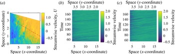
is streamwise velocity. The domain of interest was in the wake of the cylinder (see figure 1) and was composed of 221
 $y$
-direction and 441
 $x$
-direction Gauss–Legendre–Lobatto gridpoints. Temporally, the laminar data had a duration of 122 non-dimensional time units and 306 samples for a spacing of
 $\unicode[STIX]{x1D6FF}t_{L}=0.4000$
, while the turbulent data had a duration of
 $118.644$
non-dimensional time units and 724 samples for a spacing of
 $\unicode[STIX]{x1D6FF}t_{T}=0.1641$
.
(a) Shows a still frame of the fluid motion in the wake of the cylinder. The red dotted line shows the spatial extent of the data examined. (b) Shows the evolution of the laminar data through time. (c) Shows the turbulent data. Lower
 $x$
-axes show the
 $x$
-coordinate, and upper
 $x$
-axes show the (redundant)
 $y$
-coordinate as the data evolve through time.

3.1 Frequency–wavenumber analysis
For the present study, data were linearly interpolated to a one-dimensional slice in the
 $z=0$
plane having 282 spatial points, illustrated in figure 1. The spacing between points in the
 $x$
-direction was
 $0.0427d$
and in the
 $y$
-direction was
 $0.0062d$
. The endpoints of the line segment were
 $(4.0,2.75)d$
and
 $(16.0,1.0)d$
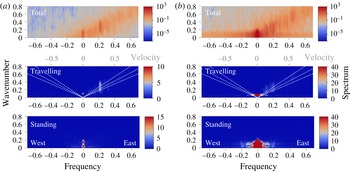
. This particular choice of domain was chosen as it bisects the opposing vortices that make up the von Kármán vortex street, as determined by visually analysing several frozen panes of flow at various times. Multitaper frequency–wavenumber spectra were computed for both the laminar and turbulent inflow conditions using
 $K=9$
and
 $5$
tapers, shown in figure 2. Figure 2(a,b) shows that standing variation (bottom axes) in both regimes appears to be concentrated mainly near the origin. Middle axes show a large amount of travelling variation, particularly along the line with velocity approximately
 $0.95d$
/time unit (white dashed line). Note also that accumulation of energy is more pronounced at the specific frequency pair
 $(0.2,0.21)$
for the laminar flow. The total spectra, defined in (2.7) and shown in the top axes, also show that turbulent-regime flows have power concentrated near zero wavenumber at high frequencies.
Multitaper frequency–wavenumber spectra are shown in the top axes of panels (a) and (b) with travelling (2.9) (middle) and standing (2.8) (bottom) axes. Travelling spectra are annotated on the upper
 $x$
-axis with velocities for the travelling waves, the white dotted lines show velocities of
 $0.75,0.95,1.15d$
units per time unit, from closest to
 $y$
-axis to farthest. Standing spectra are in the bottom axes. Note that the top (logarithmic) colour bar corresponds only to the top axes and the bottom (linear scale) colour bar corresponds to the bottom two (travelling and standing) spectra. (a) Shows frequency–wavenumber spectra for the laminar case. (b) Shows turbulent spectra computed by using 5 2-D Slepian tapers with
 $K=9$
. Total laminar spectrum shows a discrete line near
 $(f,\unicode[STIX]{x1D708})=(0.2,0.21)$
indicating a discrete oscillation with velocity
 $0.95d$
/time unit. The turbulent spectrum appears to have no such discrete line frequency.

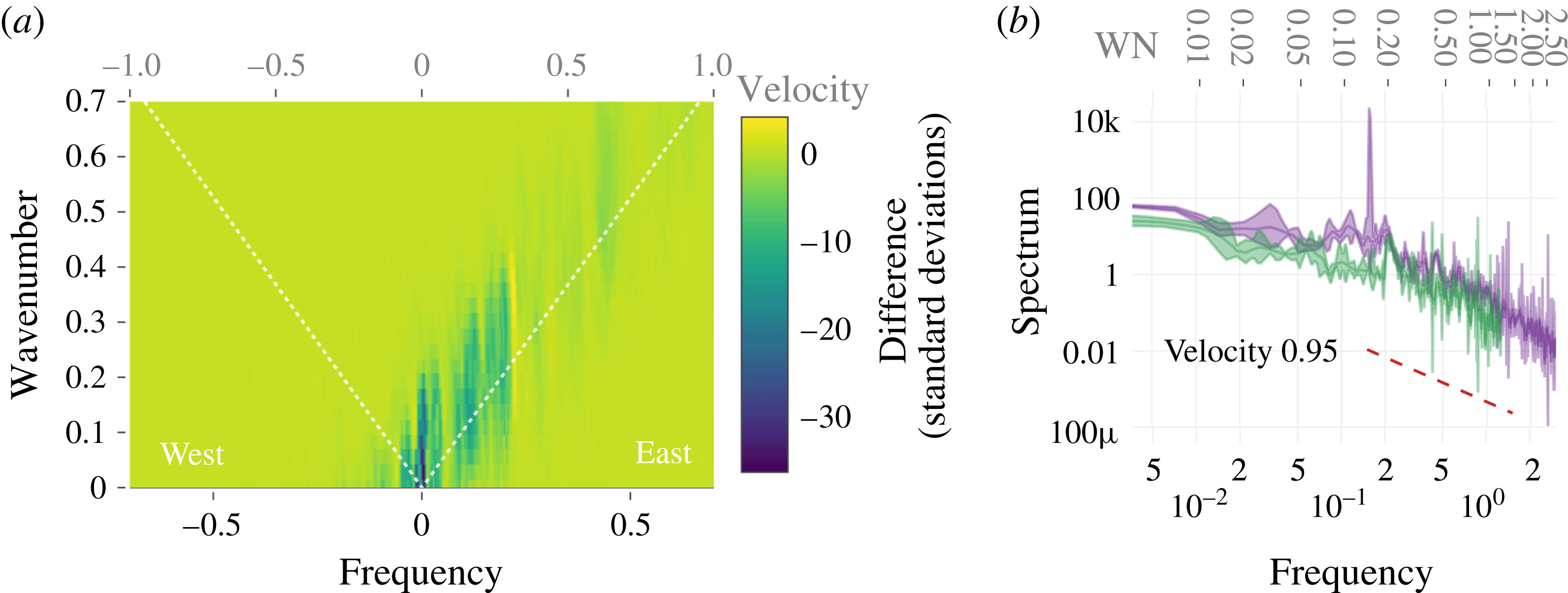
Comparing each individual pixel of the total spectrum in the two regimes, being careful to interpolate the turbulent spectrum to the same frequency grid, one obtains figure 3(a) which shows the difference between the laminar and turbulent inflow condition spectra in units of standard deviations of the laminar spectrum. In this case, we see that the largest difference between the spectra occurs near the origin and the point
 $(0.2,0.21)$
. Note that the dominant frequency of 0.2 is in contrast to the
 $St=0.1$
obtained by the authors of the original study for a different point in the geometry, outside that plotted in figure 1(a). Drawing a straight line through
 $(0,0)$
and
 $(0.2,0.21)$
and then interpolating the two total spectra along this line results in figure 3(b), which shows the laminar and turbulent spectra in green and purple, respectively, with 95 % confidence intervals annotated as semitransparent bands about the spectrum estimate. Turbulent spectra have significantly more low-frequency power through the origin to the onset of the inertial subrange, as is seen from the non-overlapping confidence limits in the
 $f\in (0,0.01)$
interval, with little overlap until
 $f=0.2$
. There is a discrete line frequency near 0.21 in the laminar inflow case which does not feature as significantly in the turbulent spectrum.
Also annotated in this panel is the
 $-5/3$
inertial range scaling regime which holds in both wavenumber and frequency. Note that there is no flattening of the spectrum in the higher frequencies which indicates we have not observed the so-called ‘noise floor’ which is usually introduced by spatial resampling.
To conclude, the present results complement the univariate spectral analysis presented in the work by Vinuesa et al. (Reference Vinuesa, Schlatter, Malm, Mavriplis and Henningson2015), where here we have found that the second harmonic of the fundamental frequency
 $St=0.1$
dominates in the region of the wake we consider. In general, univariate spectral analysis provides an incomplete description of the spatio-temporal flow characteristics, and merely summarizes the aggregate temporal information. Two-dimensional spectral analysis has enabled the quantification and visualization of standing and travelling oscillations in the two inflow scenarios.
(a) Shows a pointwise difference of the laminar and turbulent spectra in units of the estimated standard deviation of the laminar spectrum. That is, hot areas show spots where the spectra differ significantly; we see that both near the origin and at the frequency–wavenumber pair
 ${\sim}(0.2,0.21)$
there are differences. (b) Shows the interpolated spectra along the line with velocity
 $0.95d$
per time unit: purple corresponds to turbulent spectrum with 95 % confidence intervals, and green corresponds to laminar spectrum with 95 % confidence intervals. The dashed line is proportional to
 $f^{-5/3}$
, plotted approximately along the inertial subdomain. Additionally, frequency is shown on the lower
 $x$
-axis, and wavenumber is shown on the upper
 $x$
-axis.

3.2 Comparison of multitaper method with periodograms
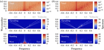
Multitaper spectra in figure 2 have a comparatively large spectral radius, as can be seen in comparison with the periodogram in figure 4. However, the periodograms have a number of features that show its inutility for scientific purposes. For one, the ‘railroad track’-shaped artefact near the line
 $(0,\unicode[STIX]{x1D708})$
shows that the periodogram window leaks power from near the origin into cross-shaped sidelobes with peaks and troughs of predictable width. Further, the periodograms are overly variable yet are not accompanied by confidence intervals. Finally, periodograms often give very negative estimates for travelling waves. As has been mentioned before, Von Storch and Zweirs point out that this decomposition is merely heuristic and that negative values cannot be taken seriously.
Periodogram frequency–wavenumber spectra for (a) laminar and (b) turbulent inflow cases. The same conventions as figure 2 have been followed.

4 Conclusions
We have introduced a fully spatio-temporal approach to the harmonic and spectral analysis of spatio-temporal flows in one space and one time dimension that additionally allows for the identification of velocities of travelling vortices and for the direct comparison of covariance structures in multiple datasets. The multitaper method we have introduced improves on naïve periodogram estimation by decreasing the bias using concentrated two-dimensional Cartesian tapers, mitigating some of the challenges that have been historically associated with multidimensional spectral density estimation.
Vortex shedding in the wake of a wall-mounted square cylinder was observed in a DNS with both laminar and turbulent inflow conditions. Using univariate spectral analysis on a time history at a single point in the geometry, one finds a single salient vortex shedding frequency (
 $St\approx 0.1$
) in the two regimes. After application of frequency–wavenumber spectral analysis, we find in the laminar case a higher energy concentration at a single frequency–wavenumber pair, corresponding to a strong discrete harmonic oscillation, whereas in the turbulent case we find a
 $-5/3$
energy cascade along a line having velocity 0.95. Additionally implied by our analysis is that the dominant vortex shedding frequency differs as a harmonic of the fundamental vortex shedding frequency in various regions of the wake.
The strength of the methods introduced here is that they allow for improved quantitative analysis and comparison of the frequency–wavenumber characteristics (standing and travelling wave interpretation) of spatio-temporal flows. In the particular example we give, one can not only determine the properties of these data, but can compare quantitatively the point estimates of the spectral densities using the bootstrapped confidence intervals, which is a useful companion method to those employing estimated optimal bases to study the data like those provided by the POD and DMD.
A number of fluid dynamics applications of this technique are apparent. Although we have demonstrated the utility of this approach for comparing two simulation outputs, one could use this technique for verification. Spectra with confidence intervals like those we show here can be computed without carefully matching the sampling properties of both processes, something unlikely to be the case given computational considerations.
Acknowledgements
The authors are grateful to R. Vinuesa and P. Schlatter from the Royal Institute of Technology (KTH), Sweden, and O. Marin from Argonne National Laboratory for providing the DNS data and advice. We also thank D. J. Thomson for advice on the statistical methodology. M.A. acknowledges partial NSF funding through awards FP061151-01-PR and CNS-1545046. This material was based upon work supported by the US Department of Energy, Office of Science, Office of Advanced Scientific Computing Research, under Award DE-SC0008603 and Contract DE-AC02-06CH11347.
Appendix A. A note on preprocessing
It is helpful to demean a time series before computing the spectrum, as the zeroth-frequency bin of the Fourier transform contains the squared sum of the entire series and can be very large relative to the signal variance, which causes a spectral window artefact to be added to the result. In higher dimensions, large power near zero frequency and/or wavenumber may produce an unwanted artefact that has the shape of the spectral window additively introduced at every bin.
Consider that very different results can be obtained by demeaning a process
 $x(t,s)$
by subtracting a sample mean computed by the following methods.
 $$\begin{eqnarray}\displaystyle \hat{\unicode[STIX]{x1D707}}^{n}(t,s) & = & \displaystyle \frac{1}{N_{t}N_{s}}\mathop{\sum }_{t=0}^{N_{t}-1}\mathop{\sum }_{s=0}^{N_{s}-1}x(t,s),\hspace{68.52008pt}\text{overall}\end{eqnarray}$$
 $$\begin{eqnarray}\displaystyle \hat{\unicode[STIX]{x1D707}}^{st}(t,s) & = & \displaystyle \frac{1}{N_{t}}\mathop{\sum }_{t=0}^{N_{t}-1}\left[x(t,s)-\frac{1}{N_{s}}\mathop{\sum }_{s=0}^{N_{s}-1}x(t,s)\right],\quad \text{spacetime}\end{eqnarray}$$
 $$\begin{eqnarray}\displaystyle \hat{\unicode[STIX]{x1D707}}^{ts}(t,s) & = & \displaystyle \frac{1}{N_{s}}\mathop{\sum }_{s=0}^{N_{s}-1}\left[x(t,s)-\frac{1}{N_{t}}\mathop{\sum }_{t=0}^{N_{t}-1}x(t,s)\right],\quad \text{timespace}.\end{eqnarray}$$
Equation (A 1) has been used to compute figure 3(a,b). However, the methods above are not advisable as these result in non-zero power on
 $f=0$
or
 $\unicode[STIX]{x1D708}=0$
. Instead we prefer to compute the cosine and sine coefficients
 $a(t,\unicode[STIX]{x1D708})$
and
 $b(t,\unicode[STIX]{x1D708})$
on the spatially demeaned series, and then demean the cosine and sine coefficients by removal of the temporal sample means.
The result is that the zeroth-frequency bin is small, but the zeroth wavenumber bin may be large. In short, it is important to explain at the outset of the computation how the zero frequency and zero wavenumber components have been removed.
Appendix B. Frequency–wavenumber analysis of a toy dataset
To illustrate the nature of the Hayashi decomposition of a two-dimensional spatio-temporal spectrum into standing and travelling components, we give two short tutorial examples here.


B.1 Example
Consider the following model equation,
 $$\begin{eqnarray}\displaystyle Y_{st}(t,s) & = & \displaystyle \cos (2\unicode[STIX]{x03C0}(0.01)t/N_{t})\cos (2\unicode[STIX]{x03C0}(0.025)s/N_{x})\end{eqnarray}$$
 $$\begin{eqnarray}\displaystyle Y_{tr}(t,s) & = & \displaystyle \cos (2\unicode[STIX]{x03C0}(0.1)t+2\unicode[STIX]{x03C0}(0.04)s)\end{eqnarray}$$
 $$\begin{eqnarray}\displaystyle x(t,s) & = & \displaystyle 2Y_{st}(t,s)+Y_{tr}(t,s)+\unicode[STIX]{x1D701}(t,s),\end{eqnarray}$$
where
 $\unicode[STIX]{x1D701}(t,s)$
is a zero-mean white noise process with variance 1. The first process is a standing wave with frequency and wavenumber
 $(f,\unicode[STIX]{x1D708})=(0.01,0.025)$
. The second is a travelling wave with frequency and wavenumber
 $(f,\unicode[STIX]{x1D708})=(0.1,0.04)$
. We simulate these processes with
 $N_{s}=306$
m spatial samples and
 $N_{t}=282$
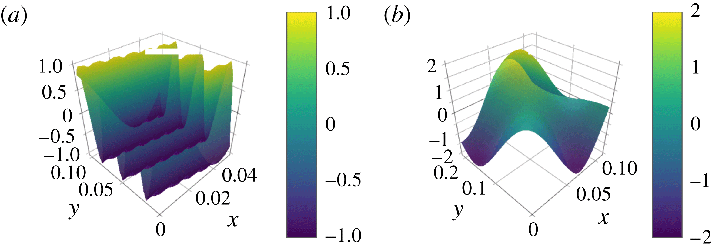
s temporal samples, a portion of which is shown in figure 5.
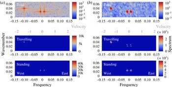
(b) Shows wavenumber–frequency multitaper spectra of the same data as (a) where a periodogram has been computed with additive unit variance white noise (B 3), where
 $K=7.0$
and 2 tapers were used. The upper plot shows the total wavenumber–frequency spectrum, the middle plot the travelling wavenumber–frequency spectrum and the bottom plot the standing wavenumber–frequency spectrum. Negative frequencies in this context are to be interpreted as westward, or opposite to streamwise traveling waves. Domain wavenumber is the number of waves that fit in the domain. The travelling wavenumber–frequency spectrum is annotated with a line of equal velocity, from closest to the origin to farthest, velocity equal to 2.5, with grey tick marks in the top of the middle axis annotating the velocities. Total spectrum is on a logarithmic scale, while travelling and standing spectra are on a linear scale, and slightly negative values saturate at zero.

The frequency–wavenumber spectra of the process
 $x(t,s)$
is shown in figure 6(a), periodogram, and 6(b), multitaper, where the spatial Fourier coefficients have been de-meaned. The travelling wave produces a pair of antisymmetric peaks in the total frequency–wavenumber diagram with amplitude
 $1/2$
. The standing component produces four peaks in the total spectrum with amplitude
 $1/4$
. From the travelling wave spectral density, one finds a peak at
 $(f,\unicode[STIX]{x1D708})=(0.1,0.04)$
, which corresponds to a wave that travels 10 m in 25 s, so the velocity is
 $2.5~\text{m}~\text{s}^{-1}$
, eastward. The travelling wave spectrum in figure 6(b) shows, in dotted white, the lines for which the velocities are the same. Annotations on the middle panel of figure 6 show lines having equal velocity at
 $2.5~\text{m}~\text{s}^{-1}$
.
B.2 Example
A simple standing pattern wave having
 $N_{s}=282$
spatial points and a domain size of 1 spatial unit, and
 $N_{t}=306$
temporal points and 1 temporal unit is generated using the formula
 $$\begin{eqnarray}\displaystyle x(t,s)=\unicode[STIX]{x1D70E}^{2}w(t,s)+\mathop{\sum }_{i=1}^{\ell }A_{i}\cos (2\unicode[STIX]{x03C0}\unicode[STIX]{x1D719}_{i}s)\cos (2\unicode[STIX]{x03C0}\unicode[STIX]{x1D713}_{i}t), & & \displaystyle\end{eqnarray}$$
where
 $\ell =2$
,
 $A_{1}=150=A_{2}$
and
 $\unicode[STIX]{x1D719}_{1}=0.2$
,
 $\unicode[STIX]{x1D719}_{2}=0.2$
and
 $\unicode[STIX]{x1D713}_{1}=0.23$
,
 $\unicode[STIX]{x1D713}_{2}=0.23$
and
 $w(t,s)$
is unit variance white noise with
 $\unicode[STIX]{x1D70E}^{2}=1$
. Thus, one expects delta function impulses at
 $(\pm 0.2,\pm 0.2)$
and
 $(\pm 0.23,\pm 0.23)$
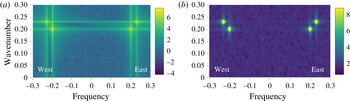
in the spectra. The periodogram and multitaper spectra with
 $K=9.0$
and 5 tapers are shown in figure 7. From the periodograms on the left-hand side, one observes large amounts of cross-shaped spectral leakage whose interference produce spurious artefacts. On the right-hand panels, the multitaper spectra in the top panel have much reduced broadband leakage, while maintaining power within a short radius. While the periodogram estimate appears to range over nearly eleven decades, the multitaper estimate ranges over just eight. The reason for this is twofold: multitaper estimators are statistically more stable than periodograms, that is, they have less variance, but when the spectrum truly contains large-power narrowband phenomena, multitaper estimators average that power over a small disk in spectral space, which results in a slight reduction in range.
(a) Shows periodograms, (b) shows multitaper (total) spectra with
 $K=9.0$
for data generated using (B 4). Note the logarithmic-base 10 colour scale. Closely spaced standing waves produce peaks having strong interference patterns. Due to the energy-concentrating properties of the Cartesian tapers, one achieves less leakage reduction at the expense of larger peak width.

For further examples, consult von Storch & Zwiers (Reference von Storch and Zwiers1999, §§ 11.5.6 and 11.5.11).
Appendix C. A note on visualization of travelling wave spectra
It is important to note that while the expressions for total and standing spectra strictly enforce positivity, the travelling wave spectrum cannot be guaranteed to be positive (von Storch & Zwiers Reference von Storch and Zwiers1999, §§ 11.3.6 and 11.5.11). In some cases this can be simply be caused by statistical fluctuations, but there are also theoretical examples which prescribe negative travelling wave variances. We emphasize that negative values in the travelling wave spectrum have no meaningful interpretation, and that the travelling wave spectrum should only be used to identify places where there is meaningful (positive) energy. On a related note, values for standing wave variance can exceed the total spectrum when the travelling wave point estimates are negative.
When one faithfully reproduces the large negative values that can result in the travelling wave spectrum, plausible features of the travelling wave spectrum become harder to identify and interpret, as the colour scale is skewed by negative estimates that have no meaning. To best visualize the positive, informative part of the travelling wave spectrum, we simply set negative values to zero, and do not modify large values in the standing component.