2.1 Inner solution – unsteady flow past a parabola

The inviscid inner solution is the flow about the rounded nose of a thin aerofoil which may be represented by a parabola. Similar to James (Reference James1983), the flow near the nose may be considered to comprise a stagnation-point point flow and a parallel (lifting) flow which results from the stagnation point moving away from the leading edge. The geometry is described in a coordinate system $(x,y)$ with the parabola nose (leading edge) coinciding with the origin, and the parabola axis (chord direction) with the $x$-axis. This problem may be elegantly solved by conformal mapping to the complex plane, shown in figure 1,

(2.1)$$\begin{eqnarray}z=rc\left(\unicode[STIX]{x1D705}-\frac{\unicode[STIX]{x1D705}^{2}}{2}\right),\end{eqnarray}$$

where $z=x+\text{i}y$, $\unicode[STIX]{x1D705}=\unicode[STIX]{x1D716}+\text{i}\unicode[STIX]{x1D702}$ and $r$ is the leading-edge radius non-dimensionalised with respect to aerofoil chord. This transformation maps the flow field in the physical $z$-plane to the left half of the $\unicode[STIX]{x1D705}$-plane. The parabola $y=\pm \sqrt{2rcx}$ is mapped to the $\unicode[STIX]{x1D716}=0$ line. The coordinates in the two planes are related as

(2.2)$$\begin{eqnarray}y=rc\unicode[STIX]{x1D702},\quad x=rc\frac{\unicode[STIX]{x1D702}^{2}}{2}.\end{eqnarray}$$

Figure 1.

(a) Unsteady flow around a parabolic curve when the stagnation point has moved away from the leading edge. (b) Transformed flow in the $\unicode[STIX]{x1D705}$-plane decomposed as stagnation flow and parallel flow.

For the stagnation-point flow, the complex velocity in the $\unicode[STIX]{x1D705}$-plane is

(2.3)$$\begin{eqnarray}\boldsymbol{v}=U_{s}(-\unicode[STIX]{x1D716}+\text{i}\unicode[STIX]{x1D702})\end{eqnarray}$$

and the velocity potential and streamfunction are

(2.4)$$\begin{eqnarray}\unicode[STIX]{x1D719}_{s}=U_{s}\frac{\unicode[STIX]{x1D702}^{2}-\unicode[STIX]{x1D716}^{2}}{2},\quad \unicode[STIX]{x1D713}_{s}=-U_{s}\unicode[STIX]{x1D716}\unicode[STIX]{x1D702}.\end{eqnarray}$$

Similarly for the parallel flow,

(2.5)$$\begin{eqnarray}\unicode[STIX]{x1D719}_{p}=U_{p}\unicode[STIX]{x1D702},\quad \unicode[STIX]{x1D713}_{p}=-U_{p}\unicode[STIX]{x1D716}.\end{eqnarray}$$

The total complex potential of the flow is given by

(2.6)$$\begin{eqnarray}F=\unicode[STIX]{x1D719}+\text{i}\unicode[STIX]{x1D713}=\left(U_{s}\frac{\unicode[STIX]{x1D702}^{2}-\unicode[STIX]{x1D716}^{2}}{2}+U_{p}\unicode[STIX]{x1D702}\right)-\text{i}(U_{s}\unicode[STIX]{x1D716}\unicode[STIX]{x1D702}+U_{p}\unicode[STIX]{x1D716}).\end{eqnarray}$$

On the aerofoil surface given by $\unicode[STIX]{x1D716}=0$, the complex potential

(2.7)$$\begin{eqnarray}F=U_{s}\frac{\unicode[STIX]{x1D702}^{2}}{2}+U_{p}\unicode[STIX]{x1D702},\end{eqnarray}$$

and turns out to be real and the same as the velocity potential.

The pressure difference across the parabola upper and lower surfaces is calculated from the unsteady Bernoulli equation,

(2.8)$$\begin{eqnarray}\frac{\unicode[STIX]{x0394}p(x)}{\unicode[STIX]{x1D70C}}=\frac{p_{l}-p_{u}}{\unicode[STIX]{x1D70C}}=\frac{1}{2}(q_{u}^{2}-q_{l}^{2})+\left(\frac{\unicode[STIX]{x2202}\unicode[STIX]{x1D719}}{\unicode[STIX]{x2202}t}\right)_{u}-\left(\frac{\unicode[STIX]{x2202}\unicode[STIX]{x1D719}}{\unicode[STIX]{x2202}t}\right)_{l},\end{eqnarray}$$

where $q_{u}$ and $q_{l}$ are total flow velocities over the aerofoil upper and lower surfaces, evaluated from $|\text{d}F/\text{d}z|$.

From the complex velocity potential derived above in (2.6), using $\unicode[STIX]{x1D716}=0$ for the aerofoil surface,

(2.9)$$\begin{eqnarray}\displaystyle & \displaystyle \frac{\unicode[STIX]{x2202}\unicode[STIX]{x1D719}}{\unicode[STIX]{x2202}t}_{\!(\unicode[STIX]{x1D716}=0)}=\frac{\dot{U_{s}}}{2}\unicode[STIX]{x1D702}^{2}+\dot{U_{p}}\unicode[STIX]{x1D702}, & \displaystyle\end{eqnarray}$$

(2.10)$$\begin{eqnarray}\displaystyle & \displaystyle \left|\frac{\text{d}F}{\text{d}z}\right|_{(\unicode[STIX]{x1D716}=0)}=\frac{U_{p}+U_{s}\unicode[STIX]{x1D702}}{rc\sqrt{1+\unicode[STIX]{x1D702}^{2}}}. & \displaystyle\end{eqnarray}$$

In the $z$-plane, $\unicode[STIX]{x1D702}=\pm \sqrt{2x/rc}$ on the aerofoil upper and lower surfaces, and

(2.11)$$\begin{eqnarray}\frac{\unicode[STIX]{x2202}\unicode[STIX]{x1D719}}{\unicode[STIX]{x2202}t}_{\!u/l}=\dot{U_{s}}\frac{x}{rc}\pm \dot{U_{p}}\sqrt{\frac{2x}{rc}}.\end{eqnarray}$$

Expressing velocities as positive going from leading edge to trailing edge on both upper and lower surfaces of the aerofoil,

(2.12)$$\begin{eqnarray}q_{u/l}=\pm \left|\frac{\text{d}F}{\text{d}z}\right|_{(\unicode[STIX]{x1D716}=0)}=\frac{U_{s}\sqrt{2x}\pm U_{p}\sqrt{rc}}{rc\sqrt{2x+rc}}.\end{eqnarray}$$

The pressure difference variation over the parabola is

(2.13)$$\begin{eqnarray}\frac{\unicode[STIX]{x0394}p(x)}{\unicode[STIX]{x1D70C}}=\frac{2\sqrt{2x}U_{s}U_{p}}{rc\sqrt{rc}(2x+rc)}+2\dot{U_{p}}\sqrt{\frac{2x}{rc}}.\end{eqnarray}$$

2.2 Outer solution – unsteady thin-aerofoil theory

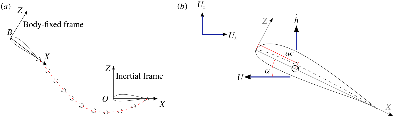
The inviscid outer solution is from an unsteady thin-aerofoil formulation based on a time-stepping approach. The method is valid for arbitrary variations in free-stream velocity and aerofoil kinematics, and contains no assumptions of small motion amplitudes or planar wakes (which are necessary in fully closed-form theories). Figure 2(a) illustrates the method, with the inertial reference frame given by $OXYZ$ and the body frame (attached to the moving aerofoil) by $Bxyz$. The two frames coincide at time $t=0$ and, at each time step, a discrete trailing-edge vortex (TEV) is shed from the trailing edge.

Figure 2.

(a) Illustration of unsteady thin-aerofoil theory and the time-stepping method. (b) Aerofoil and external velocities (positive as shown) and pitch-axis location.

The vorticity distribution over the aerofoil $\unicode[STIX]{x1D6FE}(x)$ is taken as a Fourier series,

(2.14)$$\begin{eqnarray}\unicode[STIX]{x1D6FE}(\unicode[STIX]{x1D703},t)=2U_{ref}\left[A_{0}(t)\frac{1+\cos \unicode[STIX]{x1D703}}{\sin \unicode[STIX]{x1D703}}+\mathop{\sum }_{n=1}^{\infty }A_{n}(t)\sin (n\unicode[STIX]{x1D703})\right],\end{eqnarray}$$

where $\unicode[STIX]{x1D703}$ is a variable of transformation related to the chordwise coordinate as

(2.15)$$\begin{eqnarray}x=\frac{c}{2}(1-\cos \unicode[STIX]{x1D703})\end{eqnarray}$$

and $A_{0}(t),~A_{1}(t),~\ldots ,~A_{n}(t)$ are time-dependent Fourier coefficients, $c$ is the aerofoil chord and $U_{ref}$ is a reference velocity for non-dimensionalisation chosen according to the problem. The Kutta condition (zero vorticity at the trailing edge) is enforced implicitly through the form of the Fourier series. The Fourier coefficients are determined from the instantaneous local downwash, $W(x,t)$, by enforcing the zero-normal-flow boundary condition on the aerofoil camber line,

(2.16)$$\begin{eqnarray}A_{0}(t)=-\frac{1}{\unicode[STIX]{x03C0}}\int _{0}^{\unicode[STIX]{x03C0}}\frac{W(x,t)}{U_{ref}}\,\text{d}\unicode[STIX]{x1D703},\quad A_{n}(t)=\frac{2}{\unicode[STIX]{x03C0}}\int _{0}^{\unicode[STIX]{x03C0}}\frac{W(x,t)}{U_{ref}}\cos n\unicode[STIX]{x1D703}\,\text{d}\unicode[STIX]{x1D703}.\end{eqnarray}$$

The normal downwash on the aerofoil camber line transferred to the chord line is determined from the aerofoil and free-stream velocities shown in figure 2(b),

(2.17)$$\begin{eqnarray}\displaystyle W(x,t) & = & \displaystyle \frac{\unicode[STIX]{x2202}\unicode[STIX]{x1D702}_{c}}{\unicode[STIX]{x2202}x}\left((U_{X}+u)\cos \unicode[STIX]{x1D6FC}+({\dot{h}}-U_{Z})\sin \unicode[STIX]{x1D6FC}+\frac{\unicode[STIX]{x2202}\unicode[STIX]{x1D719}_{w}}{\unicode[STIX]{x2202}x}\right)\nonumber\\ \displaystyle & & \displaystyle -\,(U_{X}+u)\sin \unicode[STIX]{x1D6FC}-\dot{\unicode[STIX]{x1D6FC}}(x-ac)+({\dot{h}}-U_{Z})\cos \unicode[STIX]{x1D6FC}-\frac{\unicode[STIX]{x2202}\unicode[STIX]{x1D719}_{w}}{\unicode[STIX]{x2202}z},\qquad\end{eqnarray}$$

where $\unicode[STIX]{x1D702}_{c}(x)$ is the camber variation on the aerofoil, $a$ is the non-dimensional location of the pitch axis from 0–1, and $\unicode[STIX]{x2202}\unicode[STIX]{x1D719}_{w}/\unicode[STIX]{x2202}x$ and $\unicode[STIX]{x2202}\unicode[STIX]{x1D719}_{w}/\unicode[STIX]{x2202}z$ are velocities induced on the camber line in directions tangential and normal to the chord by discrete vortices in the wake. Arbitrary motion kinematics of the aerofoil in the two-dimensional plane are represented by the time-varying parameters – plunge velocity in the $Z$-direction ${\dot{h}}(t)$, horizontal velocity in the $-X$-direction $u(t)$, and pitch angle $\unicode[STIX]{x1D6FC}(t)$. The velocities $U_{X}(t)$ and $U_{Z}(t)$ are the horizontal and vertical components of external flow which may also result from gusts or other perturbations. The strengths of TEVs shed at every time step are solved for such that Kelvin’s circulation condition is enforced,

(2.18)$$\begin{eqnarray}\unicode[STIX]{x1D6E4}_{B}(t)+\sum \unicode[STIX]{x1D6E4}_{TEVs}=0,\end{eqnarray}$$

where $\unicode[STIX]{x1D6E4}_{B}$ is the bound circulation, calculated by integrating the vorticity distribution (2.14) over the aerofoil chord,

(2.19)$$\begin{eqnarray}\unicode[STIX]{x1D6E4}_{B}(t)=U_{ref}c\unicode[STIX]{x03C0}\left(A_{0}(t)+\frac{A_{1}(t)}{2}\right).\end{eqnarray}$$

A detailed description of this approach and its implementation may be found in Ramesh et al. (Reference Ramesh, Gopalarathnam, Edwards, Ol and Granlund2013, Reference Ramesh, Gopalarathnam, Granlund, Ol and Edwards2014). For further discussion in this article, we assume that the aerofoil travels at a constant horizontal velocity and that there are no external disturbances. The reference velocity is taken as the horizontal velocity,

(2.20a,b)$$\begin{eqnarray}u(t)=U_{ref}=u,\quad U_{X}=U_{Z}=0.\end{eqnarray}$$

The variation of pressure difference between the upper and lower surfaces over the aerofoil ($\unicode[STIX]{x0394}p=p_{l}-p_{u}$) is again derived from the unsteady Bernoulli equation (2.8) as

(2.21)$$\begin{eqnarray}\frac{\unicode[STIX]{x0394}p(x)}{\unicode[STIX]{x1D70C}}=\left(u\cos \unicode[STIX]{x1D6FC}+{\dot{h}}\sin \unicode[STIX]{x1D6FC}+\frac{\unicode[STIX]{x2202}\unicode[STIX]{x1D719}_{w}}{\unicode[STIX]{x2202}x}\right)\unicode[STIX]{x1D6FE}(x)+\frac{\unicode[STIX]{x2202}}{\unicode[STIX]{x2202}t}\int _{0}^{x}\unicode[STIX]{x1D6FE}(x)\,\text{d}x,\end{eqnarray}$$

where the second term may be evaluated from (2.14) as

(2.22)$$\begin{eqnarray}\displaystyle \frac{\unicode[STIX]{x2202}}{\unicode[STIX]{x2202}t}\int _{0}^{x}\unicode[STIX]{x1D6FE}(x)\,\text{d}x & = & \displaystyle uc\left(\dot{A_{0}}(\unicode[STIX]{x1D703}+\sin \unicode[STIX]{x1D703})+\dot{A_{1}}\left(\frac{\unicode[STIX]{x1D703}}{2}-\frac{\sin 2\unicode[STIX]{x1D703}}{4}\right)\right)\nonumber\\ \displaystyle & & \displaystyle +\,uc\mathop{\sum }_{2,3,\ldots ,n}\frac{\dot{A_{n}}}{2}\left(\frac{\sin (n-1)\unicode[STIX]{x1D703}}{n-1}-\frac{\sin (n+1)\unicode[STIX]{x1D703}}{n+1}\right).\end{eqnarray}$$

2.3 Asymptotic matching and uniformly valid solution

Asymptotic matching of the inner and outer solutions is performed by equating them in an intermediate region where both are asymptotically valid. In this region, the value of the chordwise coordinate $x$ is small for the outer solution and large for the inner solution.

Taking the limit as $x$ and $\unicode[STIX]{x1D703}$ tend to zero in the outer solution (2.21) and expressing the result in $x$,

(2.23)$$\begin{eqnarray}\frac{\unicode[STIX]{x0394}p(x)}{\unicode[STIX]{x1D70C}}=2uA_{0}\sqrt{\frac{c}{x}}\left(u\cos \unicode[STIX]{x1D6FC}+{\dot{h}}\sin \unicode[STIX]{x1D6FC}+\frac{\unicode[STIX]{x2202}\unicode[STIX]{x1D719}_{w}}{\unicode[STIX]{x2202}x}\right)+4u\dot{A_{0}}\sqrt{cx}.\end{eqnarray}$$

Taking the limit as $x$ tends to infinity in the inner solution (2.13),

(2.24)$$\begin{eqnarray}\frac{\unicode[STIX]{x0394}p(x)}{\unicode[STIX]{x1D70C}}=\frac{\sqrt{2}U_{s}U_{p}}{rc\sqrt{rcx}}+2\dot{U_{p}}\sqrt{\frac{2x}{rc}}.\end{eqnarray}$$

Equating the expressions for pressure difference in the intermediate region from the inner and outer solutions, we obtain expressions for the stagnation flow and parallel flow velocities in terms of unsteady thin-aerofoil theory variables:

(2.25)$$\begin{eqnarray}U_{s}=rc\left(u\cos \unicode[STIX]{x1D6FC}+{\dot{h}}\sin \unicode[STIX]{x1D6FC}+\frac{\unicode[STIX]{x2202}\unicode[STIX]{x1D719}_{w}}{\unicode[STIX]{x2202}x}\right),\quad U_{p}=\sqrt{2r}\,ucA_{0}.\end{eqnarray}$$

Hence the exact solutions for pressure difference and velocity near the aerofoil leading edge (derived from the parabola) are

(2.26)$$\begin{eqnarray}\displaystyle & \displaystyle \frac{\unicode[STIX]{x0394}p(x)}{\unicode[STIX]{x1D70C}}=\frac{8u\sqrt{cx}A_{0}}{rc+2x}\left(u\cos \unicode[STIX]{x1D6FC}+{\dot{h}}\sin \unicode[STIX]{x1D6FC}+\frac{\unicode[STIX]{x2202}\unicode[STIX]{x1D719}_{w}}{\unicode[STIX]{x2202}x}\right)+4u\sqrt{cx}\dot{A_{0}}, & \displaystyle\end{eqnarray}$$

(2.27)$$\begin{eqnarray}\displaystyle & \displaystyle q=\frac{\displaystyle \sqrt{x}\left(u\cos \unicode[STIX]{x1D6FC}+{\dot{h}}\sin \unicode[STIX]{x1D6FC}+\frac{\unicode[STIX]{x2202}\unicode[STIX]{x1D719}_{w}}{\unicode[STIX]{x2202}x}\right)\pm \sqrt{c}\,uA_{0}}{\displaystyle \sqrt{x+\frac{rc}{2}}}. & \displaystyle\end{eqnarray}$$

We note that these expressions are not singular at the leading edge, and that the values of pressure and velocity at the leading edge are associated with only the first Fourier term, $A_{0}$.

A uniformly valid composite solution for pressure difference across the unsteady aerofoil is obtained from Van Dyke’s principle of MAE as ‘outer solution (2.21)’ $+$ ‘inner solution (2.13)’ $-$ ‘common part ((2.24) or (2.23))’:

(2.28)$$\begin{eqnarray}\displaystyle \frac{\unicode[STIX]{x0394}p}{\unicode[STIX]{x1D70C}} & = & \displaystyle 2u\left(u\cos \unicode[STIX]{x1D6FC}+{\dot{h}}\sin \unicode[STIX]{x1D6FC}+\frac{\unicode[STIX]{x2202}\unicode[STIX]{x1D719}_{w}}{\unicode[STIX]{x2202}x}\right)\nonumber\\ \displaystyle & & \displaystyle \times \left[A_{0}\left(\frac{4c\sin (\unicode[STIX]{x1D703}/2)}{rc+2c\sin ^{2}(\unicode[STIX]{x1D703}/2)}-\tan (\unicode[STIX]{x1D703}/4)\right)+\mathop{\sum }_{1,2,\ldots ,n}^{n}A_{n}\sin n\unicode[STIX]{x1D703}\right]\nonumber\\ \displaystyle & & \displaystyle +\,uc\left[\dot{A_{0}}(\unicode[STIX]{x1D703}+\sin \unicode[STIX]{x1D703})+\dot{A_{1}}\left(\frac{\unicode[STIX]{x1D703}}{2}-\frac{\sin 2\unicode[STIX]{x1D703}}{4}\right)\right.\nonumber\\ \displaystyle & & \displaystyle +\left.\mathop{\sum }_{2,3,\ldots ,n}\frac{\dot{A_{n}}}{2}\left(\frac{\sin (n-1)\unicode[STIX]{x1D703}}{n-1}-\frac{\sin (n+1)\unicode[STIX]{x1D703}}{n+1}\right)\right].\end{eqnarray}$$

Following the same procedure as for pressure difference, a uniformly valid solution for the tangential velocity $q$ can be derived as

(2.29)$$\begin{eqnarray}\displaystyle q_{u/l} & = & \displaystyle \mp uA_{0}\tan (\unicode[STIX]{x1D703}/4)\pm u\mathop{\sum }_{1,2,\ldots ,n}A_{n}\sin n\unicode[STIX]{x1D703}\nonumber\\ \displaystyle & & \displaystyle +\,\sqrt{\frac{x}{x+\displaystyle \frac{rc}{2}}}\left(u\cos \unicode[STIX]{x1D6FC}+{\dot{h}}\sin \unicode[STIX]{x1D6FC}+\frac{\unicode[STIX]{x2202}\unicode[STIX]{x1D719}_{w}}{\unicode[STIX]{x2202}x}\pm uA_{0}\sqrt{\frac{c}{x}}\right).\end{eqnarray}$$

The forces and pitching moment on the aerofoil, obtained by integrating the pressure difference (2.28), are unchanged from those obtained from the singular expression (2.21). The solution for the unsteady thin-aerofoil problem is still of first order, but now uniformly valid with no singularities in the primitive variables.

3.1 Velocity at leading edge and location of stagnation point

The velocity in the vicinity of an unsteady aerofoil’s leading edge is given by (2.27). This expression is seen to have a similar form to that derived for steady flow (Van Dyke Reference Van Dyke1956), with $A_{0}$ replacing a parameter that is related to the steady angle of attack. This is consistent with the fact that, in previous research (Ramesh et al. Reference Ramesh, Gopalarathnam, Edwards, Ol and Granlund2013, Reference Ramesh, Gopalarathnam, Granlund, Ol and Edwards2014), the $A_{0}$ term in unsteady thin-aerofoil theory has been shown to be an ‘effective unsteady angle of attack’ consisting of contributions from the geometric angle of attack, aerofoil camber, plunge velocity and induced velocities by the wake.

The velocity at the unsteady aerofoil’s leading edge is derived from (2.27) (or (2.29))

(3.1)$$\begin{eqnarray}q_{LE}=\sqrt{\frac{2}{r}}uA_{0}.\end{eqnarray}$$

The leading-edge velocity being proportional to $A_{0}$ is well established in unsteady thin-aerofoil theory and has previously been derived through a limit process applied at the leading edge. From Garrick (Reference Garrick1937) and von Kármán & Burgers (Reference von Kármán and Burgers1963), the form of the theoretically infinite velocity is given by

(3.2)$$\begin{eqnarray}q_{LE}=\lim _{x\rightarrow 0}\frac{S}{\sqrt{x}},\end{eqnarray}$$

where $S$ is a measure of leading-edge suction,

(3.3)$$\begin{eqnarray}S=\lim _{x\rightarrow 0}\frac{1}{2}\unicode[STIX]{x1D6FE}(x,t)\sqrt{x},\end{eqnarray}$$

which is finite and proportional to $A_{0}$ (Ramesh et al. Reference Ramesh, Gopalarathnam, Granlund, Ol and Edwards2014) when evaluated using the current thin-aerofoil formulation. This was the theoretical basis for defining the LESP equal to $A_{0}$ in Ramesh et al. (Reference Ramesh, Gopalarathnam, Granlund, Ol and Edwards2014). Asymptotic matching in this article provides a finite value of the leading-edge velocity and further reveals that it is inversely proportional to the square root of the aerofoil leading-edge radius.

The location of the stagnation point may be determined by applying the condition $q=0$. The sign of $A_{0}$ indicates the stagnation point as lying on the lower surface (if positive) or on the upper surface (if negative). If the value of $A_{0}$ (effective unsteady angle of attack) is small, the stagnation point is close to the leading edge and well approximated by a simple expression from the parabola solution (2.27):

(3.4)$$\begin{eqnarray}\sqrt{\frac{x_{s}}{c}}=\frac{u}{\displaystyle u\cos \unicode[STIX]{x1D6FC}+{\dot{h}}\sin \unicode[STIX]{x1D6FC}+\frac{\unicode[STIX]{x2202}\unicode[STIX]{x1D719}_{w}}{\unicode[STIX]{x2202}x}}A_{0}.\end{eqnarray}$$

Closed-form expressions for the leading-edge velocity and stagnation point in some simplified scenarios may be derived from (3.1) and (3.4).

3.1.1 Steady aerofoil

Considering steady flow around a thin aerofoil without camber at constant angle of attack,

(3.5)$$\begin{eqnarray}\unicode[STIX]{x1D702}_{c}=0,\quad {\dot{h}}=0,\quad \frac{\unicode[STIX]{x2202}\unicode[STIX]{x1D719}_{w}}{\unicode[STIX]{x2202}x}=\frac{\unicode[STIX]{x2202}\unicode[STIX]{x1D719}_{w}}{\unicode[STIX]{x2202}z}=0,\end{eqnarray}$$

(3.6)$$\begin{eqnarray}\displaystyle & \displaystyle A_{0}=\sin \unicode[STIX]{x1D6FC}, & \displaystyle\end{eqnarray}$$

(3.7)$$\begin{eqnarray}\displaystyle & \displaystyle q_{LE}=\sqrt{\frac{2}{r}}u\sin \unicode[STIX]{x1D6FC}, & \displaystyle\end{eqnarray}$$

(3.8)$$\begin{eqnarray}\displaystyle & \displaystyle x_{s}=c\tan ^{2}\unicode[STIX]{x1D6FC}. & \displaystyle\end{eqnarray}$$

3.1.2 Quasi-steady theory of unsteady aerofoil

Considering an unsteady aerofoil without camber and applying the quasi-steady assumption (induced velocities by wake are neglected),

(3.9)$$\begin{eqnarray}\unicode[STIX]{x1D702}_{c}=0,\quad \frac{\unicode[STIX]{x2202}\unicode[STIX]{x1D719}_{w}}{\unicode[STIX]{x2202}x}=\frac{\unicode[STIX]{x2202}\unicode[STIX]{x1D719}_{w}}{\unicode[STIX]{x2202}z}=0,\end{eqnarray}$$

(3.10)$$\begin{eqnarray}\displaystyle & \displaystyle A_{0}=\sin \unicode[STIX]{x1D6FC}-\frac{{\dot{h}}}{u}\cos \unicode[STIX]{x1D6FC}+\frac{\dot{\unicode[STIX]{x1D6FC}}c}{u}\left(\frac{1}{2}-a\right), & \displaystyle\end{eqnarray}$$

(3.11)$$\begin{eqnarray}\displaystyle & \displaystyle q_{LE}=\sqrt{\frac{2}{r}}\left(u\sin \unicode[STIX]{x1D6FC}-{\dot{h}}\cos \unicode[STIX]{x1D6FC}+\dot{\unicode[STIX]{x1D6FC}}c\left(\frac{1}{2}-a\right)\right), & \displaystyle\end{eqnarray}$$

(3.12)$$\begin{eqnarray}\displaystyle & \displaystyle x_{s}=c\left(\frac{u\sin \unicode[STIX]{x1D6FC}-{\dot{h}}\cos \unicode[STIX]{x1D6FC}+\dot{\unicode[STIX]{x1D6FC}}c(\frac{1}{2}-a)}{u\cos \unicode[STIX]{x1D6FC}+{\dot{h}}\sin \unicode[STIX]{x1D6FC}}\right)^{2}. & \displaystyle\end{eqnarray}$$

3.1.3 Theodorsen’s theory of unsteady aerofoil

In Theodorsen (Reference Theodorsen1935), an unsteady aerofoil without camber undergoes small harmonic oscillations in pitch and plunge at a reduced frequency $k=\unicode[STIX]{x1D714}c/2u$, and small-angle simplifications are applied ($\sin \unicode[STIX]{x1D6FC}\approx \unicode[STIX]{x1D6FC}$, $\cos \unicode[STIX]{x1D6FC}\approx 1$). The wake is assumed to be planar and extending to infinity, on the basis of which closed-form expressions are derived for the velocities induced by the wake on the aerofoil. The vorticity distribution on the aerofoil in Theodorsen’s theory is derived in Epps & Roesler (Reference Epps and Roesler2018). The vorticity is partitioned into a non-circulatory part $\unicode[STIX]{x1D6FE}_{n}$, a circulatory part associated with the motion $\unicode[STIX]{x1D6FE}_{c0}$ (the quasi-steady part), and a circulatory part associated with the wake $\unicode[STIX]{x1D6FE}_{w}$.

Expressing these vorticity components from Epps & Roesler (Reference Epps and Roesler2018) in terms of the chordwise transformation variable $\unicode[STIX]{x1D703}$, we have

(3.13)$$\begin{eqnarray}\displaystyle & \displaystyle \unicode[STIX]{x1D6FE}_{n}=\frac{2}{\sin \unicode[STIX]{x1D703}}\left(W_{3qc}\cos \unicode[STIX]{x1D703}-\frac{\dot{\unicode[STIX]{x1D6FC}}c}{4}(\cos \unicode[STIX]{x1D703}+\cos 2\unicode[STIX]{x1D703})\right), & \displaystyle\end{eqnarray}$$

(3.14)$$\begin{eqnarray}\displaystyle & \displaystyle \unicode[STIX]{x1D6FE}_{c0}=\frac{2W_{3qc}}{\sin \unicode[STIX]{x1D703}}, & \displaystyle\end{eqnarray}$$

(3.15)$$\begin{eqnarray}\displaystyle & \displaystyle \unicode[STIX]{x1D6FE}_{w}=-2\text{i}kW_{3qc}S(k)\left(Q_{0}(k)\frac{1+\cos \unicode[STIX]{x1D703}}{\sin \unicode[STIX]{x1D703}}+\mathop{\sum }_{n=1}^{\infty }Q_{n}(k)\sin n\unicode[STIX]{x1D703}\right), & \displaystyle\end{eqnarray}$$

where $W_{3qc}$ is the normal downwash at the aerofoil three-quarter chord location,

(3.16)$$\begin{eqnarray}W_{3qc}=u\unicode[STIX]{x1D6FC}-{\dot{h}}-\dot{\unicode[STIX]{x1D6FC}}c(a-{\textstyle \frac{3}{4}}),\end{eqnarray}$$

$S(k)$ is the Sears function,

(3.17)$$\begin{eqnarray}S(k)=\frac{1/\text{i}k}{\text{K}_{1}(\text{i}k)+\text{K}_{0}(\text{i}k)},\end{eqnarray}$$

and the wake coefficients are defined as

(3.18)$$\begin{eqnarray}Q_{n}(k)=\int _{0}^{\infty }\text{e}^{-\text{i}k\cosh \unicode[STIX]{x1D701}}\text{e}^{-n\unicode[STIX]{x1D701}}\,\text{d}\unicode[STIX]{x1D701}.\end{eqnarray}$$

The first two wake coefficients may be evaluated analytically (Epps & Roesler Reference Epps and Roesler2018) as

(3.19a,b)$$\begin{eqnarray}Q_{0}=\text{K}_{0}(\text{i}k),\quad Q_{1}(k)=\text{K}_{1}(\text{i}k)-\frac{1}{\text{i}k}\text{e}^{-\text{i}k},\end{eqnarray}$$

while the remaining terms must be calculated numerically. In the equations above, $\text{K}_{n}(\text{i}k)$ is the modified Bessel function of the second kind of order $n$.

Equating the vorticity formulation in unsteady thin-aerofoil theory (2.14) with these expressions, the equivalent Fourier coefficients are derived as

(3.20)$$\begin{eqnarray}\left.\begin{array}{@{}c@{}}\displaystyle A_{0}=C(k)\frac{W_{3qc}}{u}-\frac{\dot{\unicode[STIX]{x1D6FC}}c}{4u},\\ \displaystyle A_{1}=\frac{\dot{\unicode[STIX]{x1D6FC}}c}{2u}-2\frac{W_{3qc}}{u}(C(k)-\text{e}^{-\text{i}k}S(k)),\\ \displaystyle A_{2,\ldots ,n}=(-1)^{n}2\text{i}kS(k)\frac{W_{3qc}}{u}Q_{n},\end{array}\right\}\end{eqnarray}$$

where $C(k)$ is Theodorsen’s function, a complex number dependent on reduced frequency. This function models the induced velocity of the wake, and effects an amplitude reduction and phase shift:

(3.21)$$\begin{eqnarray}C(k)=\frac{\text{K}_{1}(\text{i}k)}{\text{K}_{1}(\text{i}k)+\text{K}_{0}(\text{i}k)}.\end{eqnarray}$$

The Fourier coefficients corresponding to Theodorsen’s theory may also be directly derived from UTAT, equations (2.16) and (2.17), by applying small-angle approximations, equating chordwise wake-induced velocity $\unicode[STIX]{x2202}\unicode[STIX]{x1D719}_{w}/\unicode[STIX]{x2202}x$ to zero (due to planar wake assumption) and calculating the chord-normal wake-induced velocity from the thin-aerofoil result (Katz & Plotkin Reference Katz and Plotkin2000),

(3.22)$$\begin{eqnarray}\frac{\unicode[STIX]{x2202}\unicode[STIX]{x1D719}_{w}}{\unicode[STIX]{x2202}z}=\frac{1}{2\unicode[STIX]{x03C0}}\int _{0}^{\unicode[STIX]{x03C0}}\unicode[STIX]{x1D6FE}_{w}\frac{\sin \unicode[STIX]{x1D703}_{0}\,\text{d}\unicode[STIX]{x1D703}_{0}}{\cos \unicode[STIX]{x1D703}_{0}-\cos \unicode[STIX]{x1D703}}.\end{eqnarray}$$

The leading-edge velocity from Theodorsen’s theory may be derived from (3.1):

(3.23)$$\begin{eqnarray}q_{LE}=\sqrt{\frac{2}{r}}\left(C(k)\left(u\unicode[STIX]{x1D6FC}-{\dot{h}}-\dot{\unicode[STIX]{x1D6FC}}c\left(a-\frac{3}{4}\right)\right)-\frac{\dot{\unicode[STIX]{x1D6FC}}c}{4}\right).\end{eqnarray}$$

The stagnation point is derived from (3.4). The chordwise wake-induced velocity is zero owing to the planar wake assumption, and the second-order term ${\dot{h}}\unicode[STIX]{x1D6FC}$ can be neglected for small amplitudes, giving the stagnation-point expression

(3.24)$$\begin{eqnarray}x_{s}=c{A_{0}}^{2}=c\left(C(k)\left(\unicode[STIX]{x1D6FC}-\frac{{\dot{h}}}{u}-\frac{\dot{\unicode[STIX]{x1D6FC}}c}{u}\left(a-\frac{3}{4}\right)\right)-\frac{\dot{\unicode[STIX]{x1D6FC}}c}{4u}\right)^{2}.\end{eqnarray}$$

The composite pressure distribution for Theodorsen’s theory is obtained from (2.28), with the Fourier coefficients given by (3.20).

For very low reduced frequencies, we note that $k\approx 0$, $C(k)=1+0\text{i}$, and all the results for Theodorsen’s method derived above become the same as those for quasi-steady theory with small-angle approximations applied.

3.2 Verification with computational fluid dynamics

Numerical verification of the results derived above is carried out using the open-source computational fluid dynamics (CFD) toolbox OpenFOAM. A body-fitted computational mesh is moved in accordance with prescribed rate laws, and the time-dependent governing equations are solved using a finite volume method. A second-order backward implicit scheme is adopted to discretise the transient terms, and second-order Gaussian integration schemes with linear interpolation for the face-centred values of the variables are used for the gradient, divergence and Laplacian terms. The pressure implicit with splitting of operators (PISO) algorithm is employed to achieve pressure–velocity coupling. This set-up has been previously used to implement the incompressible Navier–Stokes equations and study limit-cycle oscillation of a two-degree-of-freedom aerofoil (Wang et al. Reference Wang, Ramesh, Killen and Viola2018), and leading-edge vortex shedding on finite wings of different aspect ratios (Bird & Ramesh Reference Bird and Ramesh2018; Bird et al. Reference Bird, Otomo, Ramesh and Viola2019). In this research, the incompressible Euler equations are implemented in order to best match the conditions under which the theory (potential flow) is derived. This is done by considering laminar flow, with viscosity set to zero, and using a slip boundary condition for the moving aerodynamic surface. A NACA0004 section is considered, again in order to best match the thin-aerofoil assumption in theory. An O-mesh is constructed with 360 cells around the aerofoil (with a very fine resolution near the leading edge to accurately resolve the stagnation-point location), 252 cells in the wall-normal direction, and with the far field extending to 25 chord lengths in all directions from the aerofoil. The stagnation point from CFD is identified as the location on the aerofoil that is at maximum (stagnation) pressure.

3.2.1 Harmonic plunge and pitch

The expressions for stagnation point and composite pressure difference in Theodorsen’s theory derived earlier are validated against Euler CFD for a NACA0004 aerofoil using small-amplitude, harmonic, pitch and plunge kinematics.

Figure 3.

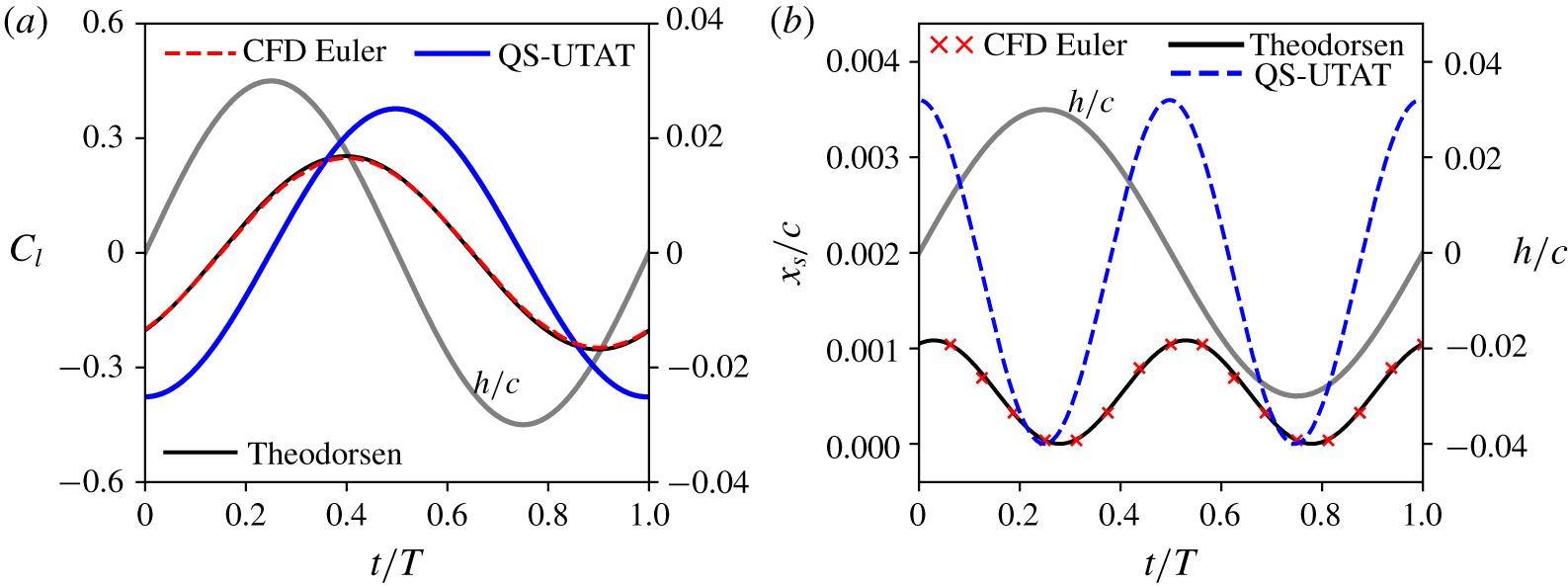
(a) Lift coefficient and (b) stagnation-point location comparison for a pure plunge case with $h_{0}=0.03$ and $k=1.0$. Plunge history is shown on the right axis of each plot.

First, a sine function of plunge is considered by taking the imaginary part of the complex motion, $h=h_{0}\text{e}^{\text{i}\unicode[STIX]{x1D714}t}$, with $h_{0}/c=0.03$ and $k=1.0$. Figure 3 shows the lift coefficient and stagnation location variations from CFD, Theodorsen’s theory and quasi-steady theory for this case. The right axis in both plots shows the plunge variation over the cycle. The quasi-steady result is shown along with Theodorsen’s to demonstrate the influence of the wake on the lift and stagnation-point locations. An excellent match between the predictions from Theodorsen and CFD is observed. We note that the lift coefficient is not affected by resolution of the leading-edge singularity and is only shown to illustrate the effect of unsteadiness (between quasi-steady and Theodorsen’s theory) and to provide a reference for the pressure distributions shown later.

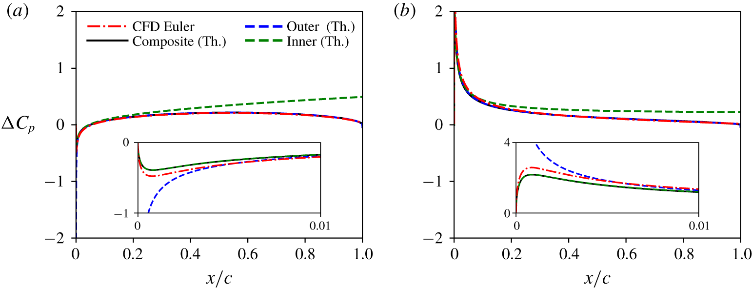
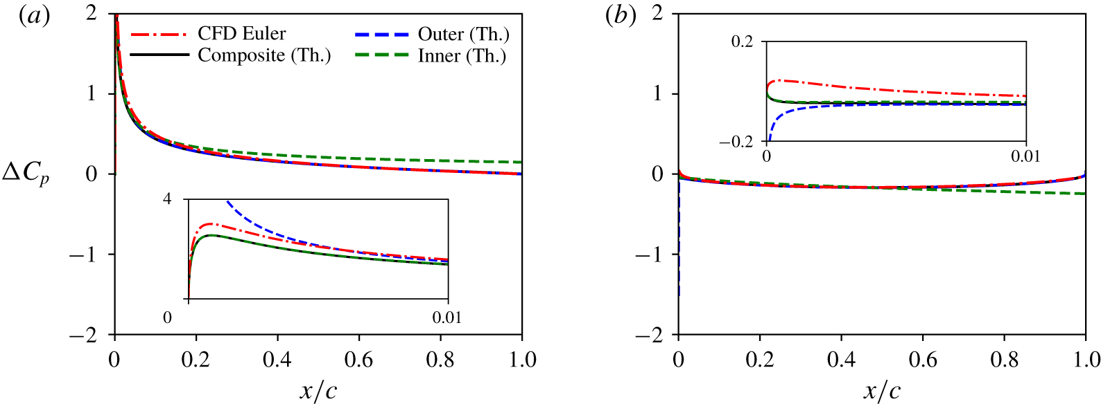
The leading-edge radius is ${\approx}0.0018c$ for a NACA0004 aerofoil. Pressure difference coefficient over the aerofoil chord from CFD is compared against the inner, outer and composite solutions from Theodorsen in figure 4. Equally spaced time instants $t/T=0.25$ and $0.5$ are shown, noting that the curves for $t/T=0.75$ and $1.0$ are the exact negatives of these owing to the symmetry in this case. The insets in these plots show the zoomed-in pressure difference near the leading edge. We observe that the composite solution is the same as the inner solution very close to the leading edge, and merges into the outer solution aft of the leading-edge radius region. The outer solution matches best with the CFD result after approximately $0.5\,\%\,c$, but goes to infinity as the leading edge is approached. The composite solution introduces a small error but correctly goes to zero at the leading edge, following the same trend as CFD. The composite solution also correctly predicts the local maxima/minima, which is reflected in the accurate prediction of stagnation-point location in figure 3.

Figure 4.

Pressure difference coefficient over the aerofoil chord for the pure plunge case from CFD and inner, outer and composite solutions from Theodorsen, at $t/T$  = (a) 0.25 and (b) 0.5. Insets show zoomed-in values at leading edge up to $1\,\%$ of chord.

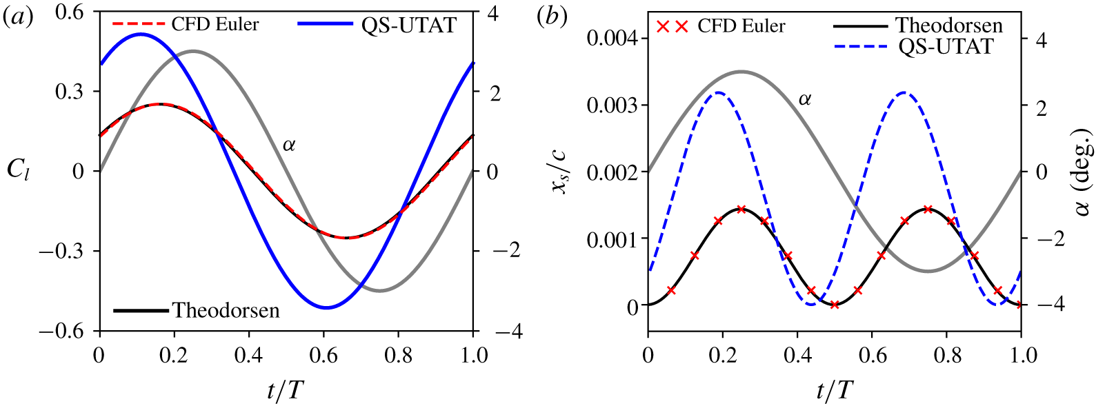
Next, a sine pitch case is considered using the imaginary part of $\unicode[STIX]{x1D6FC}=\unicode[STIX]{x1D6FC}_{0}\text{e}^{\text{i}\unicode[STIX]{x1D714}t}$ with $\unicode[STIX]{x1D6FC}_{0}=3^{\circ }$, $k=0.4$ and pitch axis at the leading edge. Figure 5 shows the lift coefficient and stagnation location variations from CFD, Theodorsen’s theory and quasi-steady theory. Excellent agreement between CFD and Theodorsen’s theory is observed. Pressure difference coefficient over the aerofoil chord from CFD is compared against the inner, outer and composite solutions from Theodorsen in figure 6, again only for the first half of the cycle owing to symmetry. Similar trends as for the plunge case are seen. The difference between CFD and the composite solution is most visible for $t/T=0.5$ (and $1.0$) where the value of $A_{0}$ is close to zero.

Figure 5.

(a) Lift coefficient and (b) stagnation-point location comparison for a pure pitch case with $\unicode[STIX]{x1D6FC}_{0}=3^{\circ }$ and $k=0.4$. Pitch history is shown on the right axis of each plot.

Figure 6.

Pressure difference coefficient over the aerofoil chord for the pure pitch case from CFD and inner, outer and composite solutions from Theodorsen, at $t/T$  = (a) 0.25 and (b) 0.5. Insets show zoomed-in pressure difference at leading edge up to $1\,\%$ of chord.

3.2.2 Ramp-up pitch manoeuvre

Next, the general unsteady thin-aerofoil theory with leading-edge correction is validated by considering a non-harmonic pitch manoeuvre. The pitch variation is defined using the Eldredge function, which produces a ramp motion with smoothed corner (Eldredge, Wang & Ol Reference Eldredge, Wang and Ol2009; Granlund, Ol & Bernal Reference Granlund, Ol and Bernal2013),

(3.25)$$\begin{eqnarray}\unicode[STIX]{x1D6FC}=\frac{K}{a_{s}}\left[\frac{\cosh (a_{s}(t^{\ast }-t_{1}^{\ast }))}{\cosh (a_{s}(t^{\ast }-t_{2}^{\ast }))}\right]+\frac{\unicode[STIX]{x1D6FC}_{0}}{2},\end{eqnarray}$$

where $a_{s}$ is a smoothing parameter defined as

(3.26)$$\begin{eqnarray}a_{s}=\frac{\unicode[STIX]{x03C0}^{2}K}{2\unicode[STIX]{x1D6FC}_{0}(1-\unicode[STIX]{x1D70E})}\end{eqnarray}$$

and

(3.27)$$\begin{eqnarray}t_{2}^{\ast }=t_{1}^{\ast }+\frac{\unicode[STIX]{x1D6FC}_{0}}{2K}.\end{eqnarray}$$

Here, $t_{1}^{\ast }$ denotes the non-dimensional time ($t^{\ast }=tu/c$) at the start of the ramp, taken as $1.0$. 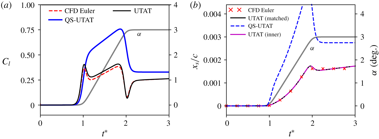The parameter $\unicode[STIX]{x1D70E}$ is a non-dimensional measure of smoothing, set to $0.8$; $\unicode[STIX]{x1D6FC}_{0}$ is the amplitude of the ramp, equal to $3^{\circ }$; and $K$ is the reduced frequency of pitch taken as $0.026$ so that the non-dimensional ramp duration is approximately equal to $1.0$. The pitch axis is located at the leading edge. The pitch history is shown on the right axis of the plots in figure 7. In this figure, lift coefficient and stagnation-point location from quasi-steady theory, unsteady thin-aerofoil theory and Euler CFD are compared. In this case, the stagnation-point $x$-location is nearly equal to the leading-edge radius of the NACA0004 aerofoil ($0.0018$) during the top of the ramp. Despite this, the stagnation points from unsteady thin-aerofoil theory calculated from both the inner solution and the full matched solution shown in figure 7 are seen to be identical. The large difference between the quasi-steady and unsteady predictions demonstrates the importance of wake-induced velocity for this case. Unlike in the previous examples, the $C_{l}$ from unsteady theory is seen to differ mildly from CFD during the ramp. There is still a very good agreement in stagnation-point prediction.

Figure 7.

(a) Lift coefficient and (b) stagnation-point location comparison for the ramp-up manoeuvre. Pitch history is shown on the right axis of each plot.

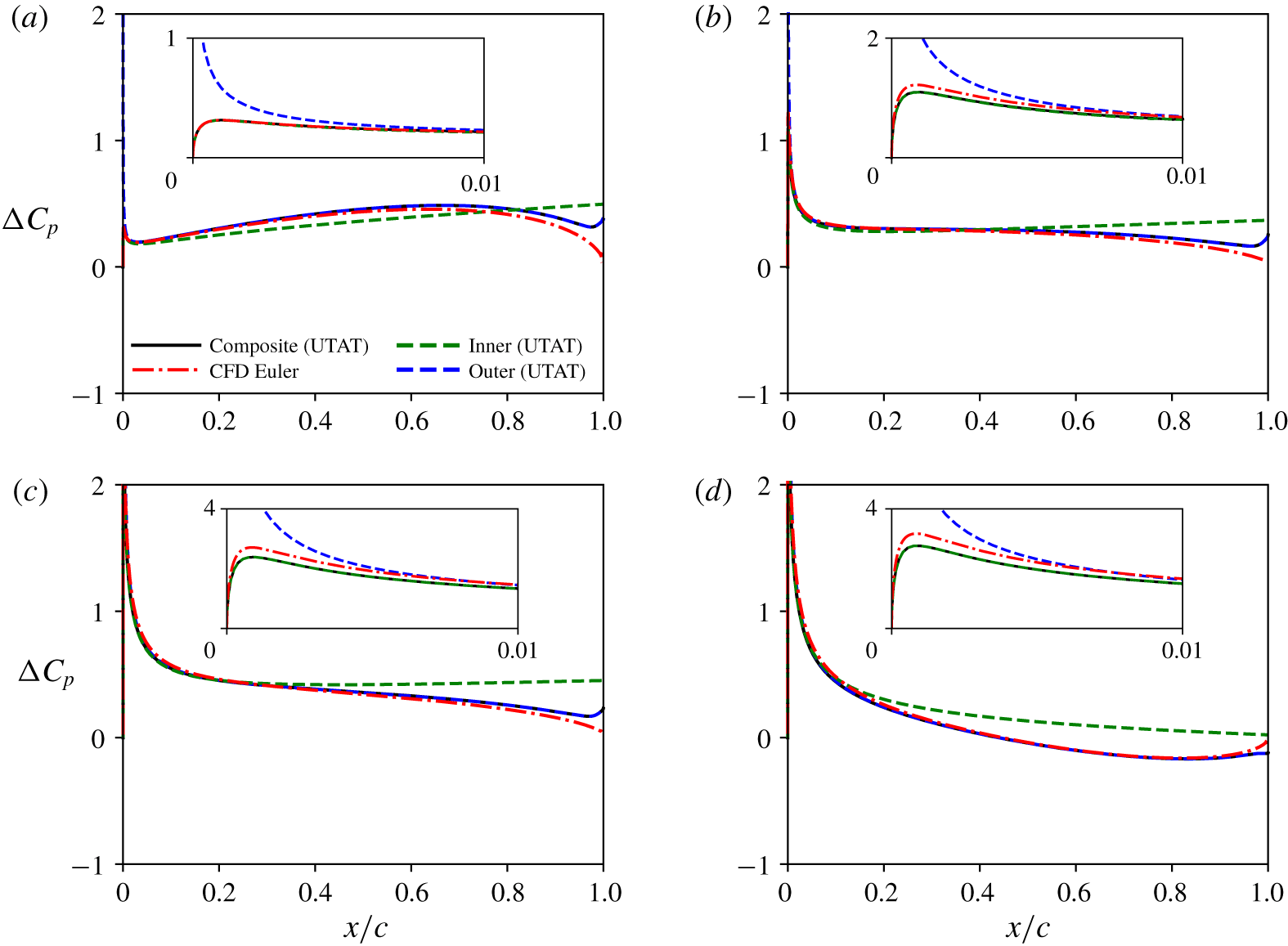
Pressure difference coefficient over the aerofoil chord from CFD and the inner, outer and composite solutions from UTAT are compared in figure 8. These plots show differences between CFD and UTAT near the trailing edge (which results in the difference in lift coefficient observed earlier), which could be related to deviations from the Kutta condition imposed in UTAT (Xia & Mohseni Reference Xia and Mohseni2017). Apart from this, there is very good agreement between the two methods, including near the leading edge.

Figure 8.

Pressure difference coefficient over the aerofoil chord for the ramp-up case from CFD and inner, outer and composite solutions from UTAT, at $t^{\ast }$  = (a) 1.0, (b) 1.25, (c) 1.75 and (d) 2.0. Insets show zoomed-in pressure difference at leading edge up to $1\,\%$ of chord.

While the validations performed above were for small-amplitude kinematics, the derivations for unsteady thin-aerofoil theory are valid for arbitrarily large amplitudes and non-planar wakes. However, for physically meaningful results, the theory must be supplemented with models/corrections to account for flow separation and vortex shedding that would occur for such kinematics, as in Ramesh et al. (Reference Ramesh, Gopalarathnam, Granlund, Ol and Edwards2014) and Narsipur, Gopalarathnam & Edwards (Reference Narsipur, Gopalarathnam and Edwards2018), for example. CFD validation must also be performed with the full Navier–Stokes equations accounting for viscous effects.