1 Introduction
In the twenty-first century, people are faced with a large number of global challenges, such as increasingly severe energy shortages, climate change, food security and major epidemic diseases. The energy crisis challenge has contributed to the emergence and development of new energy sources. Among them, solar energy is known as the best option with unique advantages including renewability, cleanness, wide applicability and economy. Solar photovoltaic technology has developed rapidly owing to crystal growth technology. Nowadays, solar cells made of monocrystalline silicon can convert solar energy into light energy directly, leading to the green energy era. In addition, the demand for high-quality, large-scale crystals in high-tech industries such as computers has become more and more urgent.
A classic method for the production of high-quality monocrystalline silicon is the Czochralski method that pulls a single crystal from the seed crystal melt (Eyer, Leiste & Nitsche Reference Eyer, Leiste and Nitsche1985). This method has been applied broadly in industrial production because of its low cost and ease of operation. The melt is crystallized on the seed crystal, and as the rod rises, a rod-shaped crystal is produced. Such a temperature distribution causes a difference in density of the silicon melt between the wall and the central part of the furnace, leading to buoyancy convection. In addition, thermocapillary convection, known as Marangoni flow, caused by surface tension, is also an important factor for the uniformity and unidirectionality in the melt crystal. It is well known that Marangoni convection will transform from a steady, axisymmetric state to an oscillatory, non-axisymmetric flow once the temperature difference exceeds a threshold. This unsteady flow can lead to the reconstruction of the crystal chemical components – stripes (microsegregation) – seriously affecting the crystal quality (Jurisch Reference Jurisch1990).
Furthermore, it is well recognized that thermocapillary convection cannot be ignored in many physical systems that involve heat/mass transmission. In-depth study of thermocapillary convection has become increasingly urgent. As a paradigmatic example of the nonlinear dynamics in essentially non-parallel flows, the flow in an annular liquid pool (LP) – simplified from the Czochralski method – has been researched numerically and experimentally under normal gravity and microgravity conditions (Kang et al. Reference Kang, Duan, Zhang, Yin, Yang and Hu2016).
Many theoretical, numerical (Li et al. Reference Li, Imaishi, Peng, Wu and Hibiya2004; Yu et al. Reference Yu, Li, Wu and Chen2015) and experimental studies (Kamotani, Ostrach & Pline Reference Kamotani, Ostrach and Pline1994; Benz & Schwabe Reference Benz and Schwabe2001) have been devoted to instability mechanisms and their characteristics have been researched. The dynamic behaviour can be characterized by the critical point, frequency, flow patterns, and so on. Smith & Davis (Reference Smith and Davis1983) first conducted a linear stability analysis in an infinitely extended thin fluid layer with an upper free surface subjected to a constant horizontal temperature gradient in the absence of gravitational force. It was discovered that the flow loses its stability with a travelling wave motion when the temperature gradient is increased. At the same time, many pure thermocapillary or thermocapillary–buoyancy convection experiments were performed with annular geometries (Renaud, Gustav & Henrik Reference Renaud, Gustav and Henrik2001), rectangular geometries (Schwabe, Benz & Cramer Reference Schwabe, Benz and Cramer1999) and open cylindrical containers (Kamotani, Lee & Ostrach Reference Kamotani, Lee and Ostrach1992). These results would help in revealing the flow instability. Burguete et al. (Reference Burguete, Mukolobwiez, Daviaud, Garnier and Chiffaudel2001) found that thermocapillary–buoyancy convection could destabilize into different patterns, depending on the temperature difference and the LP depth. The results of space experiments of an annular LP (Kamotani, Chang & Ostrach Reference Kamotani, Chang and Ostrach1994; Kamotani, Ostrach & Pline Reference Kamotani, Ostrach and Pline1995) indicated that the incipience was not solely determined by the Marangonni number, but also partly affected by the depth. Garnier & Chiffaudel (Reference Garnier and Chiffaudel2001) and Garnier, Chiffaudel & Daviaud (Reference Garnier, Chiffaudel, Daviaud, Mutabazi, Wesfreid and Guyon2006) observed hydrothermal waves (HTWs) with spiral-like shapes in a thin annular LP of 1.9 mm in depth between an inner cold rod of 8 mm in diameter and an outer wall of 135 mm in diameter. While with a depth of 1.2 mm, they found a pulsating target-like wave pattern and the cold inner rod at the centre of the cell behaved like a source of radial waves.
The studies mentioned above confirmed that many problems, including critical temperature difference and frequency, are related to the liquid surface morphology. Although space experiments can provide us the condition of producing pure thermocapillary convection, we fail to describe the free surface shape by the height of the liquid layer as the liquid could climb along the inner/outer wall under the action of surface tension. Therefore, we introduce the volume ratio Vr to study the shape effect of the fluid surface, as for LPs with certain diameters, the free surface shape could be determined by the liquid volume.
The volume ratio effect on thermocapillary convection was firstly proposed by Hu in a study of a liquid bridge, which has been proved theoretically and experimentally (Tang & Hu Reference Tang and Hu1994). The volume ratio effect in annular LPs has not been explored in depth, as the temperature field with large volume ratios is impossible to build under gravity conditions (Zhang, Duan & Kang Reference Zhang, Duan and Kang2014), where several other influential factors such as deformation, natural convection in the pool and natural convection in the ambient gas are unavoidably present. A long-period microgravity environment can provide idealistic conditions for the study of the volume ratio effect on instability mechanisms. Fortunately, we have performed space experimental research on thermocapillary convection in an annular LP on the SJ-10 satellite.
As a secondary flow in the ground environment, the thermocapillary flow experiment conducted in space is beneficial for understanding and revealing the thermocapillary convection instability mechanism. Such research can not only provide meaningful reference for crystal growth, but also deepen the study of bifurcation mechanism and turbulence in theory. The flow transition processes have been clarified, which are difficult to observe in other flows. Experiments have confirmed that the free surface forms a concave curved liquid surface instead of a convex liquid surface with increasing volume ratio. The effects of volume ratio on oscillation characteristics and transition processes have been quantitatively characterized and analysed in detail for the first time.
Due to the significant weakening of gravity, the thermocapillary flow in space is quite different from that on Earth. In a space experiment, we find that with an increasing volume ratio, in addition to periodic wave motion (Kamotani, Ostrach & Pline Reference Kamotani, Ostrach and Pline1998; Kamotani, Ostrach & Masud Reference Kamotani, Ostrach and Masud2000), the flow field could experience different transition processes. And for given values of Vr, the initial oscillation mode of an inner hot and outer cold LP is generally the standing wave, which is different from the travelling wave generated in an inner cold and outer hot LP (Shi & Imaishi Reference Shi and Imaishi2006; Peng, Li & Shi Reference Peng, Li and Shi2007). In addition, experimental results indicate that pulsating flow and rotating flow can coexist in the temperature field. The volume ratio also seriously affects the critical temperature difference, frequency, wavenumber, etc., exhibiting nonlinearity in their relationships. It has been confirmed that the frequency and wavenumber are much smaller than those of terrestrial experiment results (Zhang et al. Reference Zhang, Duan and Kang2014). The wavenumber in space no longer decreases as the liquid layer thickens (Schwabe Reference Schwabe2002; Schwabe & Benz Reference Schwabe and Benz2002), but decreasing first, then increasing and finally decreasing, which is influenced by the flow state.
2 The experimental measurement system and parameter definition
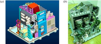
The scientific goal of the microgravity experiment ‘Space experiment on surface wave of thermocapillary convection’ performed aboard the SJ-10 satellite of China is to establish a space experiment system of thermocapillary convection in an annular (cylindrical) LP. And we aim to study the volume ratio effect for the first time, to explore instability characteristics and transition processes and to reveal in depth the instability mechanism. The internal structure and physical arrangement of the experiment equipment are shown in figure 1.
Internal structure and physical arrangement of the thermocapillary convection box. (a) The model structure and (b) the internal structure.

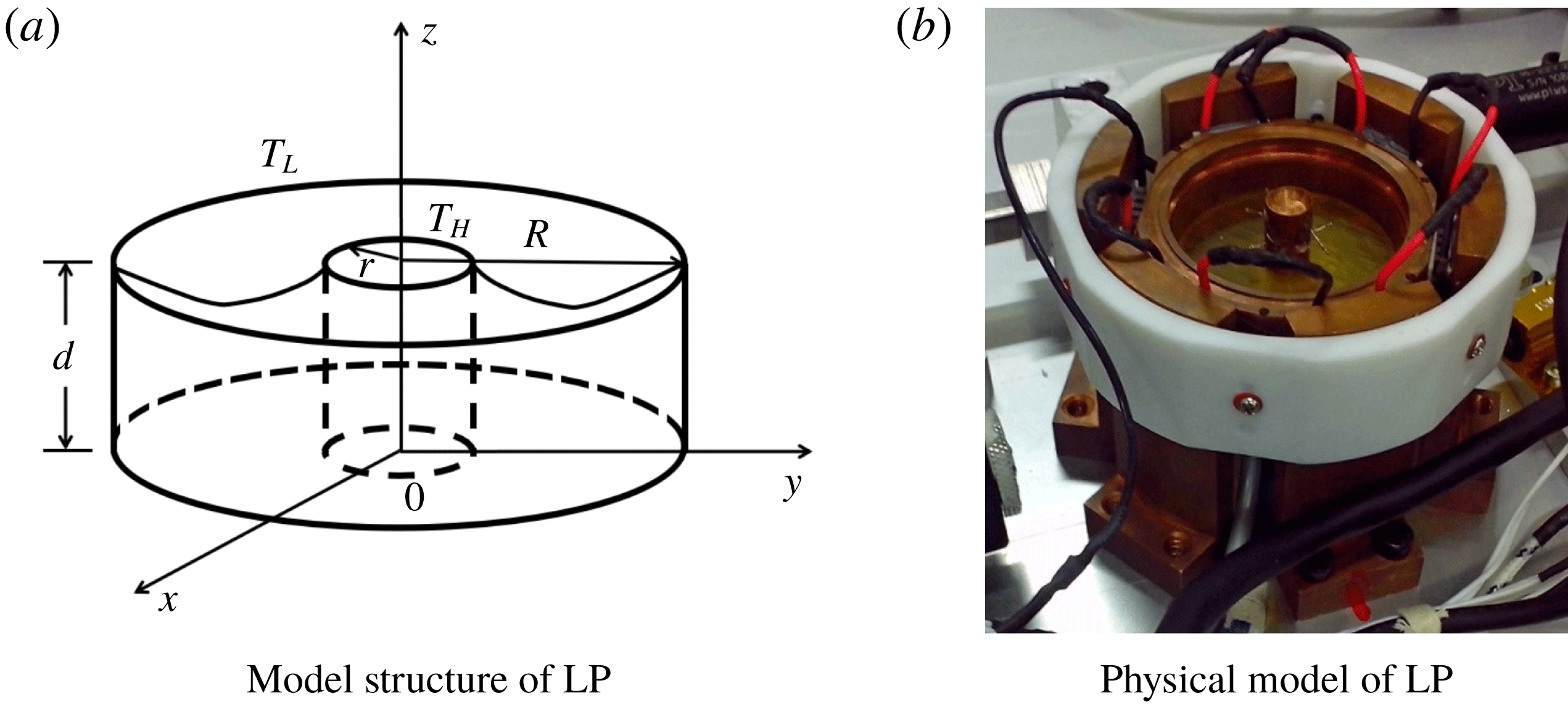
(a) Structure design and (b) physical model of the annular LP.

The thermocapillary flow system is established by heating the inner copper wall and cooling the outer copper wall of the annular LP (figure 2). And the pool is designed with outer diameter
 $R=20~\text{mm}$
, inner diameter
 $r=4~\text{mm}$
and height of the outer wall
 $d=12~\text{mm}$
. The temperature on the inner centre cylinder is defined as
 $T_{H}$
and the temperature on the outer annular wall is
 $T_{L}$
. The bottom of the LP is made of thermal insulating material with high surface flatness. A series of anti-climbing measures have been applied to maintain the liquid surface morphology before launch. On the top of the pool, non-infiltration materials are connected to copper plates with anti-climbing wedges (Kang et al.
Reference Kang, Duan, Zhang, Yin, Yang and Hu2016). The internal structure design of the LP model is presented in figure 2.
The large volume ratio can only be built in the space microgravity environment. In the experimental system, a certain volume of liquid is injected into (or sucked out of) the annular pool by a PI motor. The temperatures of the inner and outer walls are monitored and controlled by a temperature controller. There are two temperature measurement methods in this experiment, one of which uses thermocouples to measure the historical temperature at certain points, and the other adopts a thermal infrared imager to measure the entire temperature field.
A TAU2 infrared imager is applied in this experiment, its measurement sensitivity being
 $0.05\,^{\circ }\text{C}$
. The sampling frame rate is controlled at 7.5 frames per second. The temperature data are calibrated on the ground, and can be translated into an 8-bit image of a pseudo-colour display. We chose KF96 2cSt silicone oil as the working liquid for flow visualization, to observe the transition process from a steady state to oscillation with increasing temperature difference. Its relevant physical parameters are given in table 1. The temperature dependency of the kinematic viscosity of the working fluid is evaluated from the following equation:
 $$\begin{eqnarray}\displaystyle & \displaystyle \frac{\unicode[STIX]{x1D708}}{\unicode[STIX]{x1D708}_{25}}=\exp \left(5.892\frac{25-T}{273.15+T}\right), & \displaystyle\end{eqnarray}$$
 $$\begin{eqnarray}\displaystyle & \displaystyle \unicode[STIX]{x1D708}=\frac{\unicode[STIX]{x1D708}(T_{H})+\unicode[STIX]{x1D708}(T_{L})}{2}, & \displaystyle\end{eqnarray}$$
where
 $v_{25}$
and
 $T$
are the kinematic viscosity at
 $25\,^{\circ }$
C and the temperature considered, respectively.
Physical properties of KF96 2cSt silicone oil at
 $25\,^{\circ }$
C.

In our experiment, the applied temperature difference is increased at a rate of
 $0.5\,^{\circ }$
C per minute. To calculate the critical temperature difference
 $\unicode[STIX]{x0394}T_{c}$
, we utilize the fact that the oscillating temperature amplitude increases as the square root of the distance from the bifurcation point, i.e.
 $A\sim (\unicode[STIX]{x0394}T-\unicode[STIX]{x0394}T_{c})^{1/2}$
. By calculating the amplitude at some supercritical values of
 $\unicode[STIX]{x0394}T$
, we can obtain the critical threshold (Kang et al.
Reference Kang, Duan, Zhang, Yin, Yang and Hu2016).
In addition to temperature difference, there are many factors that can greatly influence the flow, which include the geometries of the liquid layer, such as the radii
 $r$
,
 $R$
, the liquid volume
 $V$
, the depth
 $d$
; and the physical properties of the fluid, such as the diffusion coefficient
 $\unicode[STIX]{x1D6FC}$
, the volume thermal diffusivity
 $\unicode[STIX]{x1D705}$
, the kinematic viscosity coefficient
 $\unicode[STIX]{x1D708}$
, the density
 $\unicode[STIX]{x1D70C}$
, the surface tension temperature coefficient
 $\unicode[STIX]{x1D70E}_{T}$
. These factors are combined into non-dimensional parameters with different physical meanings to determine the flow state. These are:
Volume ratio
 $Vr=V/V_{0}=V/\unicode[STIX]{x03C0}(R^{2}-r^{2})d$
, which is used to describe the volume ratio effect of the fluid.
Prandtl number
$Pr=\unicode[STIX]{x1D708}/\unicode[STIX]{x1D6FC}$
, is the characterization of momentum flow and heat exchange in the fluid flow.Marangoni number
$Ma=\unicode[STIX]{x1D70E}_{T}(R-r)(T_{H}-T_{L})/\unicode[STIX]{x1D70C}\unicode[STIX]{x1D708}\unicode[STIX]{x1D705}$
, which is used to characterize the driving effect of the surface tension. The Marangoni number at the critical point is commonly called the critical Marangoni number,
$Ma_{c}$
.



3 Experimental results and discussion
3.1 The flow pattern transition
An infrared thermal imager is applied to obtain the temperature distribution of the liquid free surface, since a thermocouple is limited to a single-point temperature measurement. As Vr decreases, the flow pattern transition in the annular LP can be categorized into three types of processes by the fluctuation characteristics.
For
 $Vr>0.81$
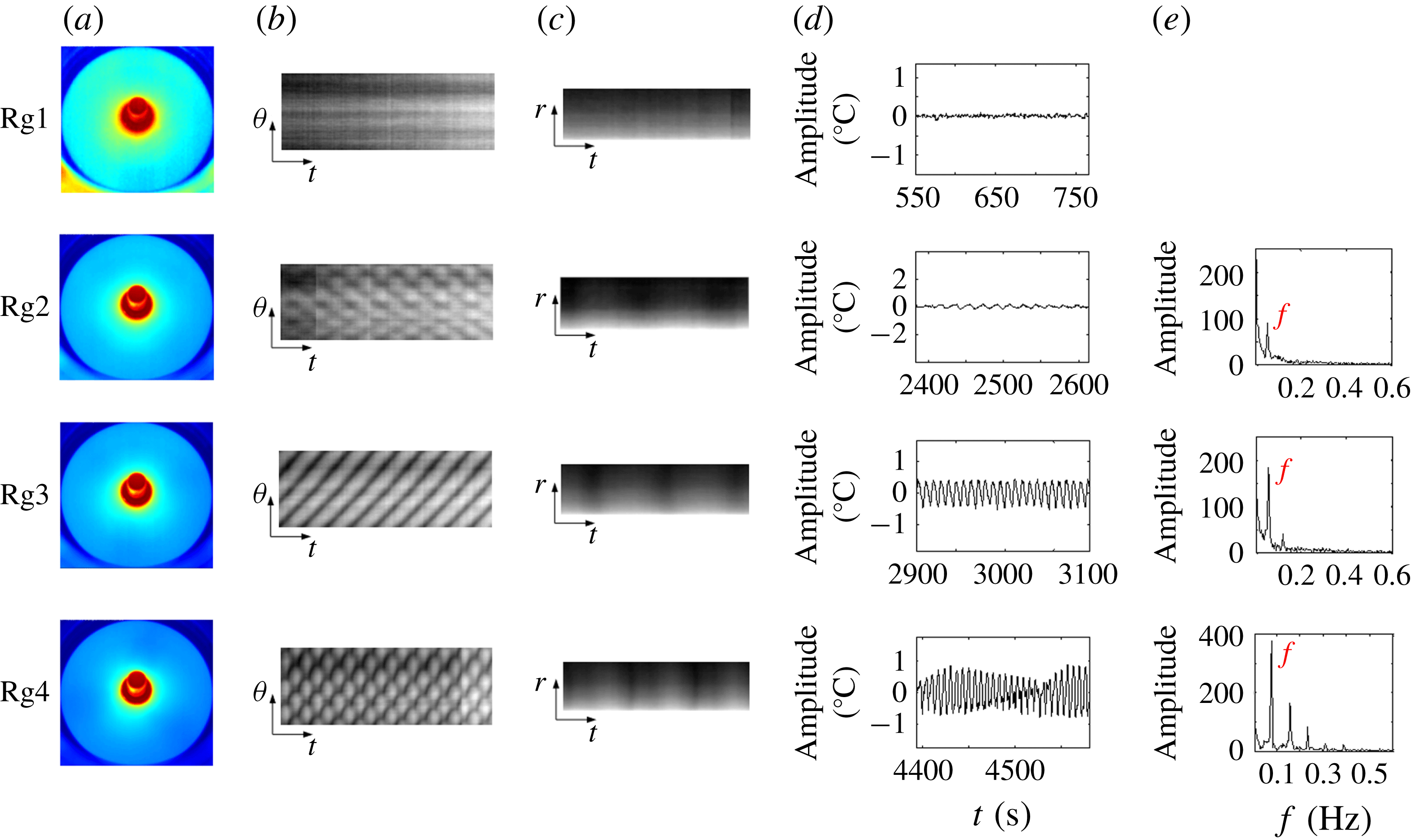
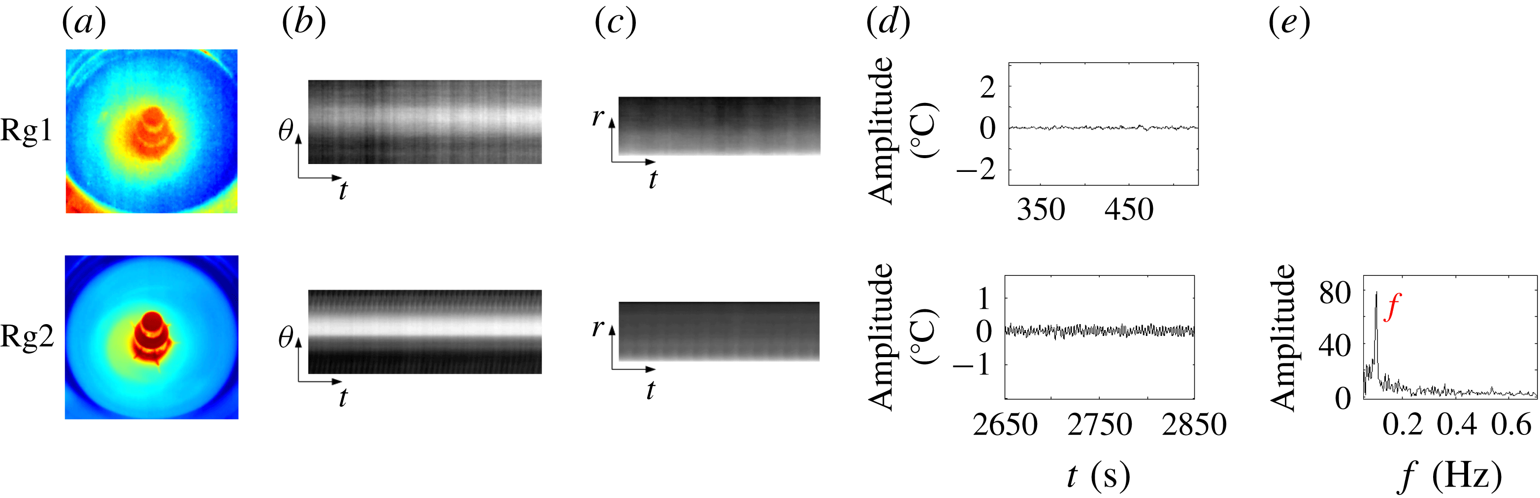
, according to different waveforms in the temperature field, the flow will experience four regimes in the pattern transition: steady; standing wave (SW); travelling wave (TW); and SW coupled with TW (figure 3). The change in colour from red to blue in the infrared image represents the variation from high temperature to low temperature. The grey-scale images are used to illustrate the temperature level: bright indicates higher temperature and dark indicates lower temperature.
The flow pattern transition for
 $Vr=0.86$
: (a) infrared images, (b) temperature–time evolution (circumferential), (c) temperature–time evolution (radial), (d) temperature signal, (e) Fourier transform. Rg1:
 $Ma=4.44\times 10^{4}$
(
 $\unicode[STIX]{x0394}T=4.74\,^{\circ }$
C); Rg2:
 $Ma=1.91\times 10^{5}$
(
 $\unicode[STIX]{x0394}T=20.36\,^{\circ }$
C); Rg3:
 $Ma=2.33\times 10^{5}$
(
 $\unicode[STIX]{x0394}T=24.94\,^{\circ }$
C); Rg4:
 $Ma=3.48\times 10^{5}$
(
 $\unicode[STIX]{x0394}T=37.13\,^{\circ }$
C).

In Rg1 (i.e.
 $Ma/Ma_{c}<1$
), a stable temperature field is created with a small
 $\unicode[STIX]{x0394}T$
, displaying a (two-dimensional) axisymmetric ‘steady’ flow (see figure 3). At the beginning of heating, the liquid surface has a thick temperature boundary layer with a small temperature gradient. The circular coaxial isotherms are uniformly distributed in the temperature field (figure 3
a). It is demonstrated by the annular and striped isotherms in the temperature–time evolution graphs (figure 3
b,c) that the fluid circles in the radius–cylindrical axis (
 $r$
–
 $z$
) plane. The temperature decreases gradually from the hot end to the cold end in the radial direction. The single-point temperatures extracted from the original infrared files (figure 3
d) resemble a horizontal line, neglecting extremely small environmental disturbances.
The boundary between Rg1 and Rg2 has already been recognized as the critical point of the flow transition from a two-dimensional steady flow to a three-dimensional time-dependent flow. When
 $1.00<Ma/Ma_{c}<1.20$
, the flow enters into Rg2, as shown in figure 3, and the convective field indicates a certain modal structure. The annular isotherm in Rg1 near the heating cylinder is transformed into a closed polygonal structure. In this process, a fixed wavenumber
 $m$
emerges in the temperature field, which does not evolve with time, and the entire temperature field is divided into
 $2m$
blocks along the radial direction from the cold end to the edge of the polygon. The two neighbouring cells respectively represent cold and heat regions, and appear in pairs. The waves exhibit azimuthal motion in addition to the movement in the
 $r$
–
 $z$
plane. There is radial temperature oscillation on the liquid free surface, and the temperature field energy is continuously transferred from the inner wall to the cold wall. The heat transmission speed increases with increasing
 $\unicode[STIX]{x0394}T$
. And the transmission effect is indicated by the periodic change of darkness in the circumferential temperature–time evolution diagram (figure 3
b) and SW motion is the interfered result of two waves propagating in the opposite direction with the same frequency. Fluctuation with obvious periodic variations of light and dark stripes in the radial evolution also indicates that there is periodic oscillation in this regime. Single-point temperature history presents as a sinusoidal oscillatory state, and the fundamental frequency
 $f=0.06$
Hz appears in the spectrum (figure 3
e). The critical instability waveform of LPs with heated inner wall and cooled outer wall is a SW, rather than a TW (Peng et al.
Reference Peng, Li and Shi2007) with cooled inner wall and heated outer wall, which confirms that the heating method can make a difference in the flow pattern transition.
With increasing Ma, the second transition emerges in the temperature field. In Rg3,
 $1.20<Ma/Ma_{c}<1.22$
, the polygonal zone in the pool rotates azimuthally along a certain direction. The isothermal lines separating cold and hot regions become inclined, and the wave has a peripheral motion component, expressed by the periodic variation of the stripe grey-scale propagating along the oblique direction in the temperature–time evolution diagram. As the pool model is axisymmetric, the TW rotating direction is uncertain, seriously influenced by the concentricity, parallelism and heating uniformity of the two walls. Similar to the SW motion, the TW motion in this regime also has a certain wave number,
 $m$
. The energy in the pool is transferred from the hot wall to the cold wall in the radial direction accompanied by circumferential transmission, and the transfer rate becomes faster and faster. The appearance period of the radial light and dark stripes has been shortened. The further developed convection lead to an increase in the amplitude and the frequency of the sinusoidal temperature oscillation.
With further increasing Ma above
 $1.22Ma_{c}$
, in Rg 4, far away from the critical oscillation state, rather than directly translating into chaos (Zhang et al.
Reference Zhang, Duan and Kang2014), a unique flow pattern is firstly recognized in the temperature field. Maintaining the wavenumber in Rg3, the amplitude and frequency of the periodic oscillation are further amplified. Rotating in the circumferential direction, this novel HTW also makes a pulsating motion in the temperature field (figure 3
a). And it should be noted that all these well-organized flow patterns including the SW, TW and this unique HTW are hardly destroyed once they are formed. Motion analysis of the temperature–time evolution indicates that the light and dark stripe structure in Rg4 becomes more complicated than that in Rg3. There is no shift of the wave node in the SW-type pulsating flow with time, and the line where all wave nodes are located is parallel to the time line in Rg2 (figure 3
b). However, superposing over the existing TW-type rotating motion, the wave nodes in this regime can shift with the fluid flow. The straight line where all wave nodes are located and the time axis have a certain angle in the circumferential temperature–time evolution diagram. The observation of this novel HTW indicates that different waveforms or at least the SW and the TW can coexist in the temperature field, without affecting each other’s motions. This ‘harmonious’ coexistence should be ascribed to the disappearance of gravity.
The LP with large volume ratios provides ‘fertile soil’ for the development of various HTWs. For
 $0.65<Vr<0.81$
, the liquid layer becomes thinner gradually, the rigid walls impose a strong constraint to the appearance and spreading of the axial waves and the flow pattern transition process (steady–SW–TW–SW coupled with TW) is broken (figure 4). Limited by the maximum
 $\unicode[STIX]{x0394}T$
that the space experiment equipment can offer, the flow can only transit from the steady state to the SW state. In Rg1, similar to Rg1 in the case mentioned above, there is a steady flow in the temperature field. While in Rg2, the SW movement is disturbed in the circumferential direction, behaving with asymmetric characteristics in the temperature–time evolution. The surface temperature shows a non-axisymmetric distribution, the isotherms become no longer smooth (figure 4
a) and the radial temperature changes without significant periodicity (figure 4
c).
Underdeveloped flow pattern transition for
 $Vr=0.78$
: (a) infrared images, (b) temperature–time evolution (circumferential), (c) temperature–time evolution (radial), (d) temperature signal, (e) Fourier transform. Rg1:
 $Ma=2.50\times 10^{5}$
(
 $\unicode[STIX]{x0394}T=2.67\,^{\circ }$
C); Rg2:
 $Ma=3.26\times 10^{5}$
(
 $\unicode[STIX]{x0394}T=34.84\,^{\circ }$
C).

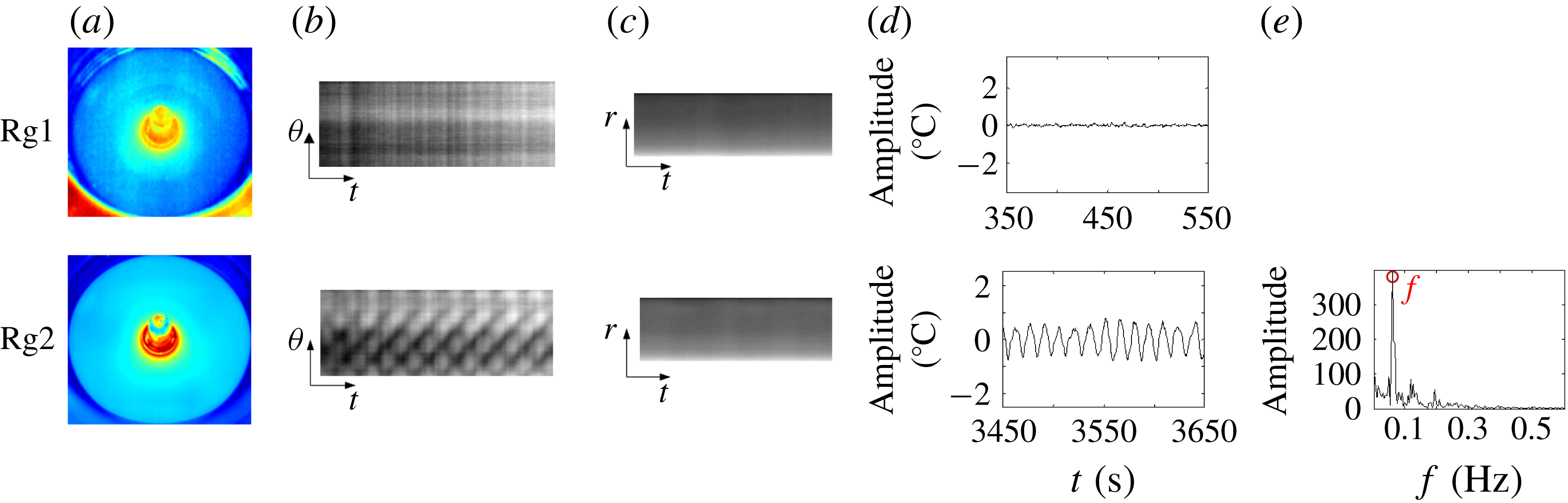
Local oscillatory flow pattern transition for
 $Vr=0.42$
: (a) infrared images, (b) temperature–time evolution (circumferential), (c) temperature–time evolution (radial), (d) temperature signal, (e) Fourier transform. Rg1:
 $Ma=3.1\times 10^{4}$
(
 $\unicode[STIX]{x0394}T=3.28\,^{\circ }$
C); Rg2:
 $Ma=2.1\times 10^{5}$
(
 $\unicode[STIX]{x0394}T=22.42\,^{\circ }$
C).

When the thickness of the liquid layer is below a certain value,
 $Vr<0.65$
, the effect of the rigid walls is increased. The flow pattern transition in the temperature field becomes extremely different. Once above the critical point, previous steady flow in the temperature field evolves into local oscillation (figure 5). The fluid in the oscillating region still makes a periodic motion with a higher frequency
 $f=0.1$
Hz. Far from this area, the temperature field is steady without any oscillation (figure 5
d). The centres of the annular isotherms deviate from the heating column, meaning that the temperature distribution in the circumferential direction is non-uniform. The wave that flows towards the cold wall and the wave that bounces back from the rigid wall influence each other, so no flow pattern could be recognized in the flow field.
The wave motion in the LP is a continuous process of energy concentration and dissipation. There are two waves propagating in opposite directions in the temperature field throughout the transition process. If these two waves accumulate the same amount of energy, they form a pulsating motion. Once one of the waves gathers more energy, the flow will transform into a rotating motion. When the energy of the two waves is almost the same before the chaotic state, SW-type movement emerges in the temperature field.
In order to verify the above results, the amplitude equation is calculated by Landau theory according to the nature of the flow field, to explore the instability mechanism and the appearance of TW and SW in weak nonlinear analysis. First, the wave propagating in the counterclockwise direction in the flow field is simplified as
 $$\begin{eqnarray}W(\unicode[STIX]{x1D703},t)=\text{A}_{+}\cos (m\unicode[STIX]{x1D703}-wt),\end{eqnarray}$$
where
 $\unicode[STIX]{x1D703}$
is the circumferential azimuth.
Similarly, clockwise waves can be described as
 $$\begin{eqnarray}W(\unicode[STIX]{x1D703},t)=\text{A}_{-}\cos (-m\unicode[STIX]{x1D703}-wt).\end{eqnarray}$$
A simplified model of the two waves whose amplitude satisfies the Landau equation is
 $$\begin{eqnarray}\displaystyle \displaystyle \unicode[STIX]{x2202}A_{+}/\unicode[STIX]{x2202}t=\unicode[STIX]{x1D70E}A_{+}-(\unicode[STIX]{x1D6FD}|A_{+}|^{2}+\unicode[STIX]{x1D6FE}|A_{-}|^{2})A_{+}, & & \displaystyle\end{eqnarray}$$
 $$\begin{eqnarray}\displaystyle \displaystyle \unicode[STIX]{x2202}A_{-}/\unicode[STIX]{x2202}t=\unicode[STIX]{x1D70E}A_{-}-(\unicode[STIX]{x1D6FD}|A_{-}|^{2}+\unicode[STIX]{x1D6FE}|A_{+}|^{2})A_{_{-}}, & & \displaystyle\end{eqnarray}$$
where
 $\unicode[STIX]{x1D70E}$
is the growth rate of the amplitude. When
 $\unicode[STIX]{x1D70E}>0$
, it means that the flow field oscillates. Here
 $\unicode[STIX]{x1D6FD}$
and
 $\unicode[STIX]{x1D6FE}$
are their own nonlinear action and the mutual one, respectively.
On analysis of these two equations, when
 $A_{+}=0$
,
 $A_{-}=0$
, it means that the flow field is steady; when
 $A_{+}\neq 0$
,
 $A_{-}=0$
or
 $A_{+}=0$
,
 $A_{-}\neq 0$
, the flow field expresses a clockwise/counterclockwise wave motion, that is, a TW motion, and the corresponding amplitude is obtained as
 $A=\sqrt{\unicode[STIX]{x1D70E}/\unicode[STIX]{x1D6FD}}$
.
When
 $A_{+}=A_{-}$
, the flow field expresses a SW motion, and the corresponding amplitude is obtained as
 $A_{+}=A_{-}=\sqrt{\unicode[STIX]{x1D70E}/(\unicode[STIX]{x1D6FD}+\unicode[STIX]{x1D6FE})}$
.
Assume
 $\unicode[STIX]{x1D6FD}>0\,\unicode[STIX]{x1D6FE}>0$
: when
 $\unicode[STIX]{x1D6FE}<\unicode[STIX]{x1D6FD}$
, the flow field selects SW motion, and when
 $\unicode[STIX]{x1D6FE}>\unicode[STIX]{x1D6FD}$
, the flow field selects TW motion. Here
 $\unicode[STIX]{x1D6FD}$
and
 $\unicode[STIX]{x1D6FE}$
change with increasing temperature difference, thereby causing a transition from a TW motion to a SW motion or from a SW motion to a TW motion.
Considering that the flow field just begins to oscillate, the amplitude is relatively small,
 $A\rightarrow 0$
. The nonlinear influence is very weak, the temperature is exponentially increasing and its characteristic time is
 $O(1/\unicode[STIX]{x1D70E})$
. At the onset of the oscillation, the growth rate
 $\unicode[STIX]{x1D70E}$
tends to be
 $0^{+}$
. Therefore, the characteristic time is greater than the oscillation period
 $(O(1/\unicode[STIX]{x1D70E})>2\unicode[STIX]{x03C0}/w)$
and an unsteady SW transition region appears before the TW is fully developed.
According to the experimental results, we select
 $\unicode[STIX]{x1D70E}=0.1$
,
 $\unicode[STIX]{x1D6FD}=100$
and
 $\unicode[STIX]{x1D6FE}=200$
to calculate the oscillation process by the Landau equation. The
 $A_{+}$
curve and the
 $A_{+}$
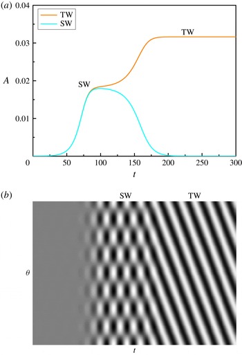
curve have been obtained by the fourth-order Runge–Kutta method, and the spatio-temporal evolution diagram is shown in figure 6. There is a transient region – SW motion – in the thermocapillary convection process.
Weak nonlinear analysis. (a) The amplitude curve. (b) The spatio-temporal evolution diagram.

In the experiment, a short-time SW motion is observed in the initial stage for most experiments, and the time evolution graph is qualitatively consistent with the simulation result in figure 6. The SW amplitude is relatively small, and it is an unstable transition oscillation. With the flow fully developing, the field makes a long-term TW motion.
The generating conditions of SW and TW have attracted extensive interest. It has been clarified that TW is the stable solution for thermocapillary convection with
 $Pr>4$
(Leypoldt, Kuhlmann & Rath Reference Leypoldt, Kuhlmann and Rath2000). And it is a feature of thermocapillary convection in a liquid with large
 $Pr$
that SW motion is the initial oscillation state, even though the initial perturbation introduced into the system was non-symmetric (Muehlner et al.
Reference Muehlner, Schatz, Petrov, Swift and Swinney1997). However, considering all factors, the initial perturbations of ground experiments, space experiments and numerical simulation are different.
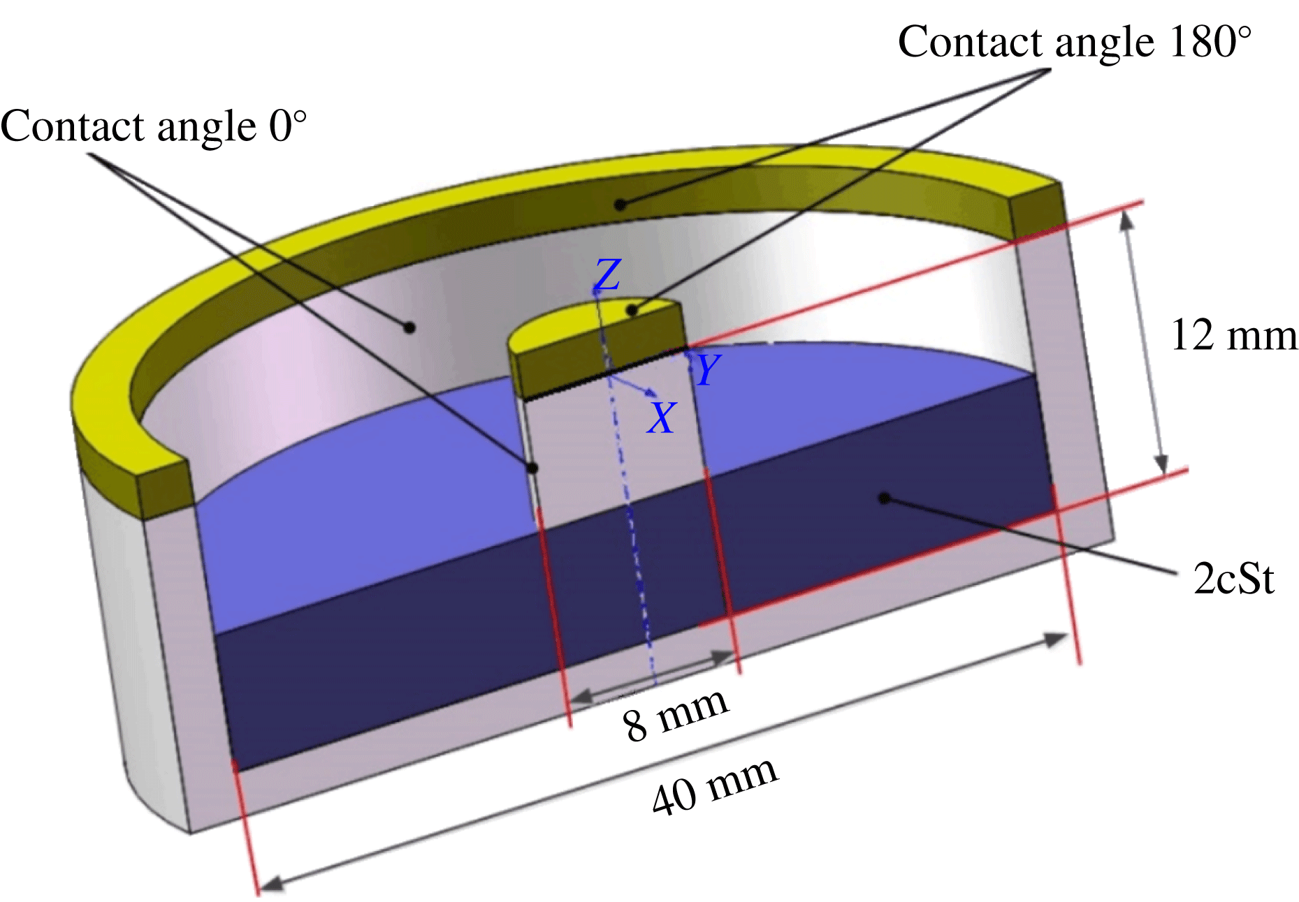
These differences in the transition process should be ascribed to the volume ratio. The fluid volume determines the shape of the gas–liquid surface, introducing a difference in the temperature distribution, which greatly affects the fluid movement. We fail to obtain the liquid surface topography in the present space experiments due to the limitations of measurement methods, so the liquid surface topographies corresponding to different volume ratios are numerically simulated in this paper. Figure 7 shows the model numerically simulated by FLOW-3D software based on the multiphase volume of fluid method. The liquid surfaces corresponding to the values of Vr in figures 3–5 are obtained by simulation, and the influence of shape on flow patterns is further analysed.
In order to simulate the wedge structure of the LPs, a solid wall with a contact angle of
 $180^{\circ }$
to the silicone oil is placed on the surface of the centre cylinder and the surface of the annular side wall to achieve an anti-climbing effect. The numerical calculations are performed with the following basic assumptions:
(1) The liquid is incompressible with constant viscosity and density that are not affected by temperature and time.
(2) Heat exchange between the container and the liquid is not considered.
(3) Microgravity in the space environment is at the level of
$10^{-3}g$
. The liquid is filled from the bottom of the container at the initial time.

The boundary conditions are as follows:
(1) The fluid does not slip relative to the wall, which means that the two velocity components on the surface of the wall are zero.
(2) The fluid does not penetrate through the wall, which that means that the velocity component perpendicular to the boundary surfaces of the annular side wall and the centre cylinder is zero.
(3) The normal stress equilibrium condition and the tangential stress equilibrium condition are applied on the gas–liquid interface.
Due to the large proportion of surface tension in the numerical model, a hexahedral grid is adopted. The total number of grids is 1.55 million, and the average grid spacing is 0.25 mm.
The model diagram of numerical simulation.

The position of a phase in space is obtained by solving the volume fraction of a certain phase in the entire computational space, and the volume fraction of the liquid phase satisfies the equation
 $$\begin{eqnarray}\frac{\unicode[STIX]{x2202}F}{\unicode[STIX]{x2202}t}+\boldsymbol{v}\boldsymbol{\cdot }\unicode[STIX]{x1D735}F=0,\end{eqnarray}$$
where
 $F=F$
(
 $x$
,
 $y$
,
 $z$
) is the fluid volume function, which represents the volume fraction occupied by the fluid in the calculated region. By calculating the volume change of the fluid in a grid unit and the volume ratio function
 $F$
of the grid unit, we can track the fluid movement. If
 $F=0$
, the unit is occupied by the gas-phase fluid; if
 $F=1$
, the unit is occupied by the liquid-phase fluid; if
 $0<F<1$
, the unit contains fluid in two phases. The
 $F$
function is set at the centre of the cell, and the velocity of the fluid is set at the four sides of the grid cell. To determine the position and shape of the free surface in the free-surface element, the fluid volume flowing through the grid cell is calculated by the fluid volume functions of adjacent grid cells and the fluid velocities on the four sides of the mesh cell.
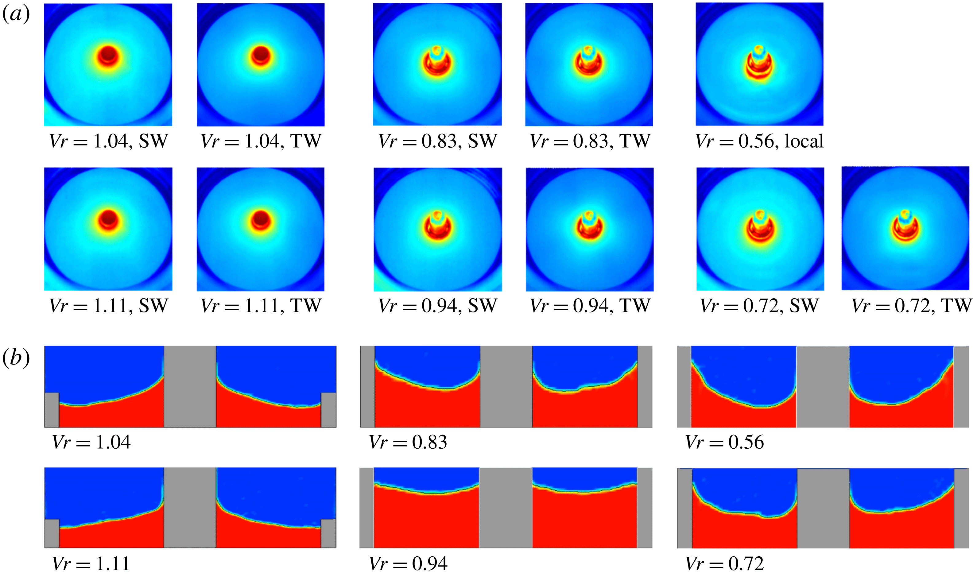
(a) The free-surface temperature distribution of thermocapillary convection. (b) The calculated liquid surface morphology at
 $10^{-3}~\text{g}$
.

An overview of the infrared images for various volume ratios is presented in figure 8(a). And the corresponding gas–liquid interface morphology simulation results are shown in figure 8(b). The free-surface morphology in the annular LP is mainly decided by the surface tension generated by the temperature difference imposed on the walls. A meniscus with a large curvature is formed on the gas–liquid interface in thermocapillary convection by the surface tension.
The liquid in the pool is pulled towards the heating/cooling wall by the surface tension. And there is a notable change in the morphology of the free surface as Vr increases. The temperature gradient of the free surface increases during the transition process, further affecting the morphology of the free surface. Marangoni convection is the result of a combination of force and heat, coupled with temperature and velocity. Consequently, this change in the morphology has a strong influence on the flow state.
For
 $Vr=0.56$
, the height of the liquid climbing at the outer wall is higher than that at the inner one. And the increasing volume makes the liquid climb along the heating column (
 $Vr=0.72$
). Limited by the heating and the cooling walls, there is a meniscus between the two walls, and its curvature gradually becomes smaller with more liquid (
 $Vr=0.83,0.94$
). Interestingly, when the volume ratio exceeds a certain value, the liquid will submerge the heating column and then climb along the central axis. The liquid surface maintains a concave surface (
 $Vr=1.04$
, 1.11), rather than a convex surface as in terrestrial gravity.
It is seen that the deformation of the LP shape owing to gravity is remarkable for all values of Vr especially for the large ones. This may suggest that the difference in the Vr effect on the instability between terrestrial gravity and microgravity is a direct consequence of the change of LP shape. The volume ratio partly determines the morphology of the liquid surface, greatly affecting the fluid motion characteristics such as wavenumbers, which will be discussed in detail later.
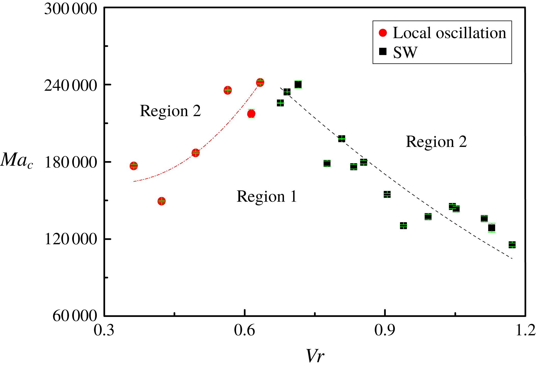
Critical Marangoni number corresponding to different volume ratios (
 $0.36<Vr<1.17$
). Region 1 is the steady flow and region 2 is the oscillatory flow.

3.2 Critical temperature difference and frequency
Marangoni convection is generated by the temperature difference imposed on the walls. The onset of oscillation is determined through flow visualization based on the infrared camera. The volume ratio effect on
 $Ma_{c}$
for the critical oscillation is plotted in figure 9. This figure is divided into two regions according to the flow states. One is the steady-state region (region 1) and the other is the oscillation region (region 2). With increasing Ma, a steady laminar flow of region 1 transits to an oscillatory three-dimensional flow of region 2. As a function of Vr, the critical curve is divided into two branches, showing strong nonlinear characteristics. The features reported in this research are that (1) the convection becomes most stabilized at certain Vr at around 0.65 and (2) the vibrational states observed in critical conditions are different between
 $Vr<0.65$
and
 $Vr>0.65$
. When
 $Vr>0.65$
, periodic oscillation appears in the temperature field, leading to certain modal structures in Rg2, and more well-organized flow patterns in Rg3 and even other regimes. And
 $Ma_{c}$
is inversely proportional to increasing Vr. As shown in figure 8, the thickening of the liquid layer reduces the curvature of the liquid surface, the surface energy of the liquid becomes smaller, so that the system requires less energy to destabilize the steady flow.
When
 $Vr<0.65$
, the field fails to generate the polygonal structure even when Ma exceeds the threshold value (figure 5). Irregularly distributed isotherms indicate the emergence of local oscillation. And the system needs more energy to undermine periodic movement with increasing volume ratio, and
 $Ma_{c}$
increases noticeably. It is demonstrated that the reconstruction of the flow field is attributed to the flow pattern transition, and the differences of the flow field structures make the instability features different.
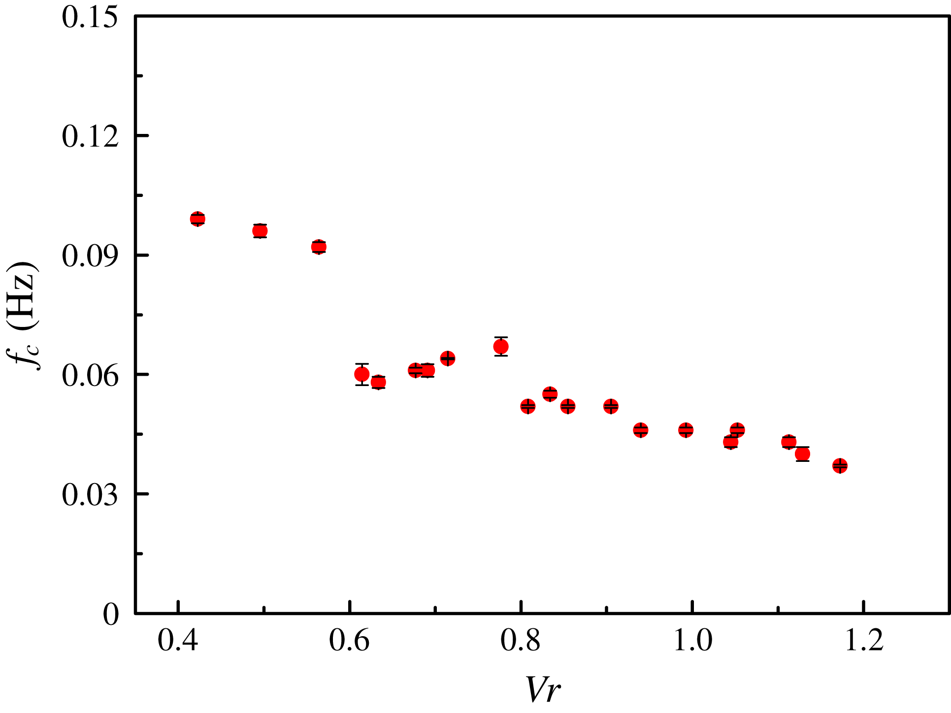
As an important physical parameter that characterizes the periodic motion, figure 10 shows the critical frequency,
 $f_{c}$
, plotted as a function of Ma. This indicates that
 $f_{c}$
partly depends upon the volume ratio. The thickening of the fluid layer makes the movement period longer, resulting in a decrease in frequencies. The critical frequency negatively depends on the liquid volume ratio.
Critical frequencies under different volume ratios (
 $0.42<Vr<1.17$
).

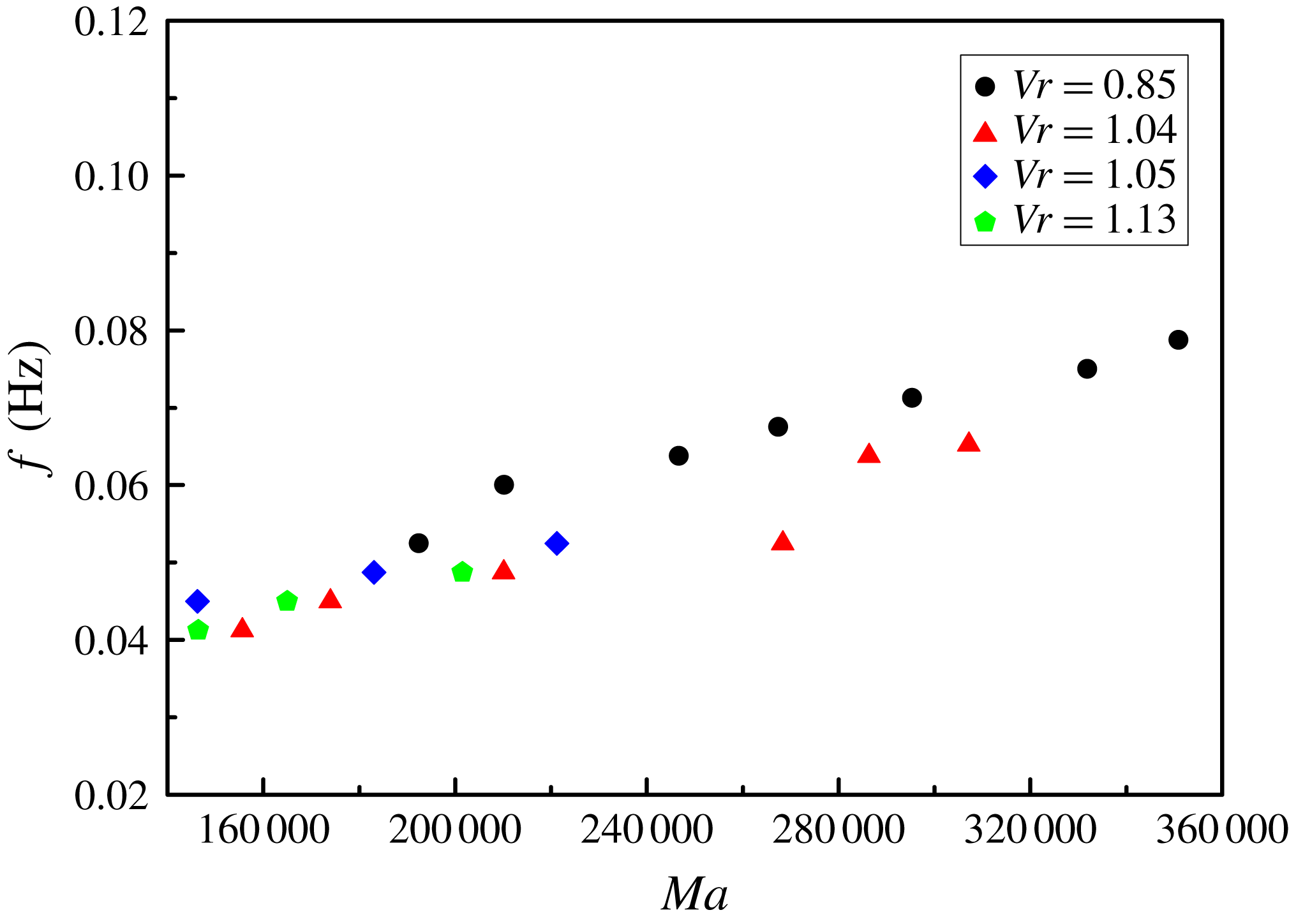
In the space experiment, driven by the surface tension, the liquid flows from the warmer side to the cooler side of the liquid–gas interface, and the back flow is generated by the conservation of mass. The oscillatory data obtained in microgravity maintain of the order of 10
 $^{-2}$
, which is much different from the data obtained on the ground (i.e.
 $1g$
), owing to the significant effect of gravity on the instability. More detailed inspection of figure 11 demonstrates that there is a sudden decrease around
 $Vr=0.6$
, where the frequency of the thin liquid layer with
 $Vr<0.6$
is much higher than that of the thick one with
 $Vr>0.6$
. This decrease can be ascribed to the appearance of periodic motion in the field. It demonstrates that Vr affects the flow field structure, and further determines the fluid movement.
As the thermal motion in the pool continues to accelerate, the frequency can be expressed as a function of Ma. In figure 11, Ma for various Vr shows a monotonically increasing behaviour, which is in good agreement with the ground experimental result (Zhang et al. Reference Zhang, Duan and Kang2014). The linear fitting slope of the frequency with the variable is in the range 0.001–0.002, and there is no notable difference between the results of different volume ratios. This reveals that the frequency is very sensitive to Ma, while practically independent of the volume ratio.
Relation between frequency and temperature difference.

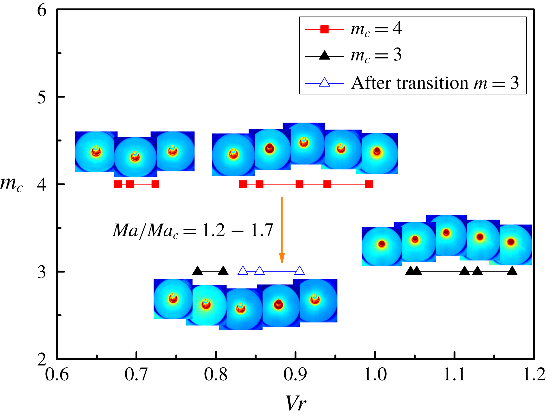
Wavenumbers under different volume ratios.

Wavenumber versus temperature difference: (a)
 $Vr=0.94$
; (b)
 $Vr=0.85$
.

3.3 The selection of wavenumber
The HTWs, which are developed owing to the unstable flow, are described by the integer values of the azimuthal wavenumber,
 $m$
. Commonly, above the critical point, a three-dimensional oscillation starts as a finite-amplitude periodic wave motion, and
 $m$
at the threshold is defined as the critical mode,
 $m_{c}$
. In the HTWs, the thermal field is strongly coupled with the velocity field, which depends on Vr and Pr among other factors. It has been suggested that the two branches of the stability diagram (
 $Ma_{c}$
versus Vr) should correspond to different
 $m$
(Shevtsova et al.
Reference Shevtsova, Mojahed, Melnikov and Legros2003). However, the surface tension causes a large deformation of the liquid surface, resulting in the critical mode in LPs remaining obscure.
In figure 12,
 $m_{c}$
exhibits an inverted ‘N’-type distribution with increasing Vr, demonstrating strong nonlinear characteristics. For
 $Vr<0.75$
and
 $0.81<Vr<1.0$
, the critical modes are 4, while
 $m_{c}$
decreases to 3 for
 $0.75<Vr<0.81$
and
 $Vr>1.0$
. This distribution characteristic should be attributed to surface tension. When the volume is small, the fluid is pulled towards the cooler side by the surface tension, and the thin liquid layer has a wavenumber of 4. Due to the limitation of the outer wall height, more liquid also begins to gather near the heating column, leading to the thickening of the liquid layer. And once the liquid volume exceeds a certain value, the liquid submerges the heating column and starts to climb along the centre column, causing the changes in
 $m_{c}$
with the increasing Vr.
The wavenumber can characterize the flow field structure under a certain temperature difference. It is revealed in figure 12 that the flow field transition with increasing temperature difference may cause a decrease in wavenumber. In the volume ratio range of 0.83 to 0.91, the wavenumber decreases from
 $m=4$
to
 $m=3$
when Ma is
 $1.2Ma_{c}$
–
 $1.7Ma_{c}$
. This means that there are fewer hot and cold zones in the temperature field as the surface temperature gradient enlarges (Zhang et al.
Reference Zhang, Duan and Kang2014). And the reconstruction of the flow field causes the original flow to be destroyed, and a new flow state is formed after transition.
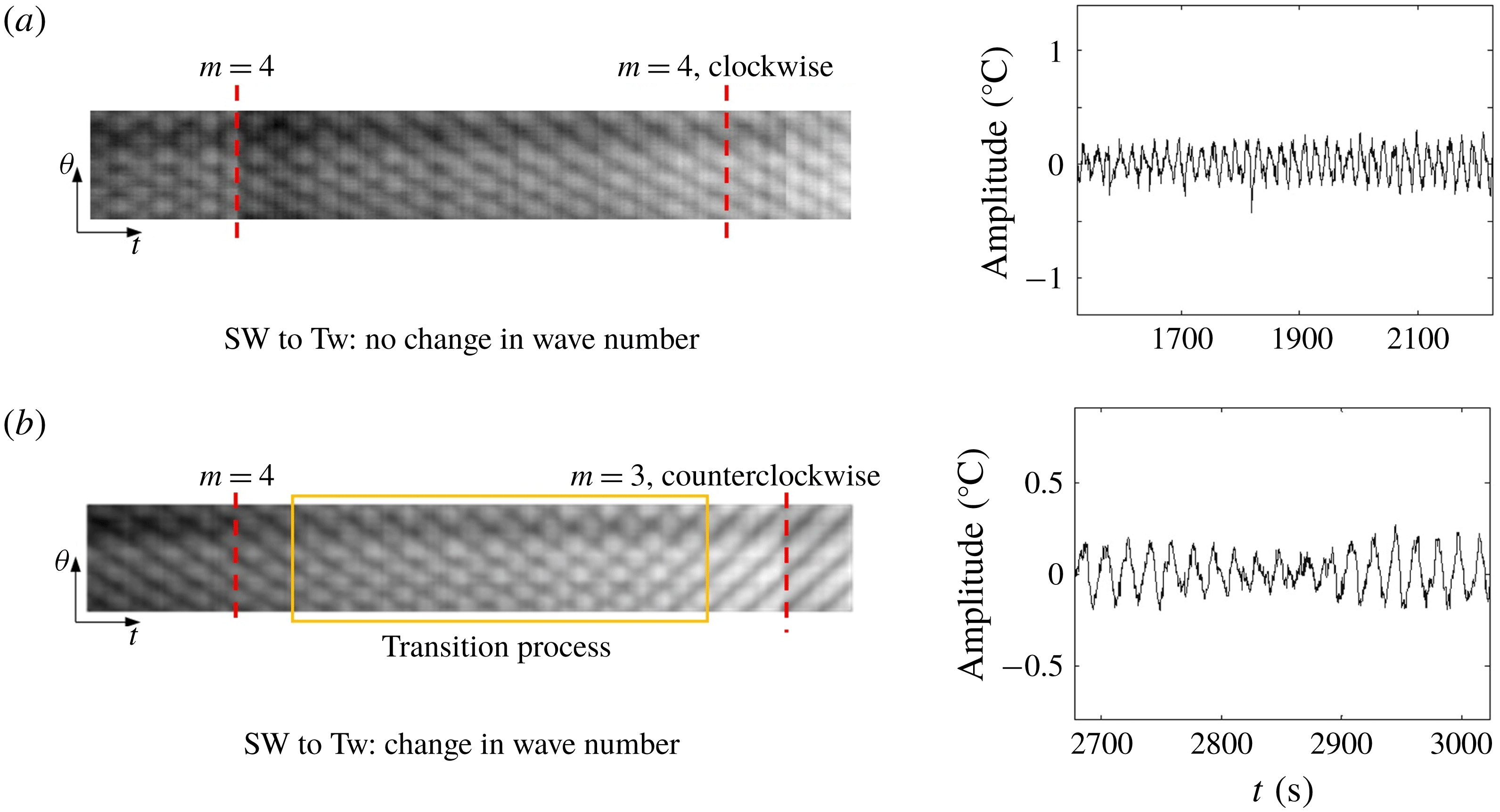
The relation between wavenumber and propagation direction of the HTWs is illustrated in figure 13. As Ma increases, the SW motion gradually evolves into a TW motion with constant
 $m$
, propagating in the clockwise direction, for
 $Vr<0.83$
or
 $Vr>0.91$
. It is well known that the reduction of the wavenumber could appear in TW flow. However, not only being decreased by increasing
 $\unicode[STIX]{x0394}T$
(Shi & Imaishi Reference Shi and Imaishi2006), in the space experiment the change of the flow state also could cause the reduction of the wavenumber. An exception is observed at a volume ratio of 0.83–0.91. The SW with
 $m=4$
fails to evolve directly to the TW with
 $m=4$
, but becomes another TW with
 $m=3$
after a transition process, and reverses its propagating direction to counterclockwise. And the change of
 $m$
only occurs in the transition process from SW to TW for given values of Vr, that is to say, the change of the wavenumber means that the SW motion in the flow field is transformed into TW motion. Wavenumbers are closely related to the flow state.
The relation between propagation angle and Marangoni number for
 $Vr=0.85$
.

The relation between propagation angle and Marangoni number for various volume ratios.

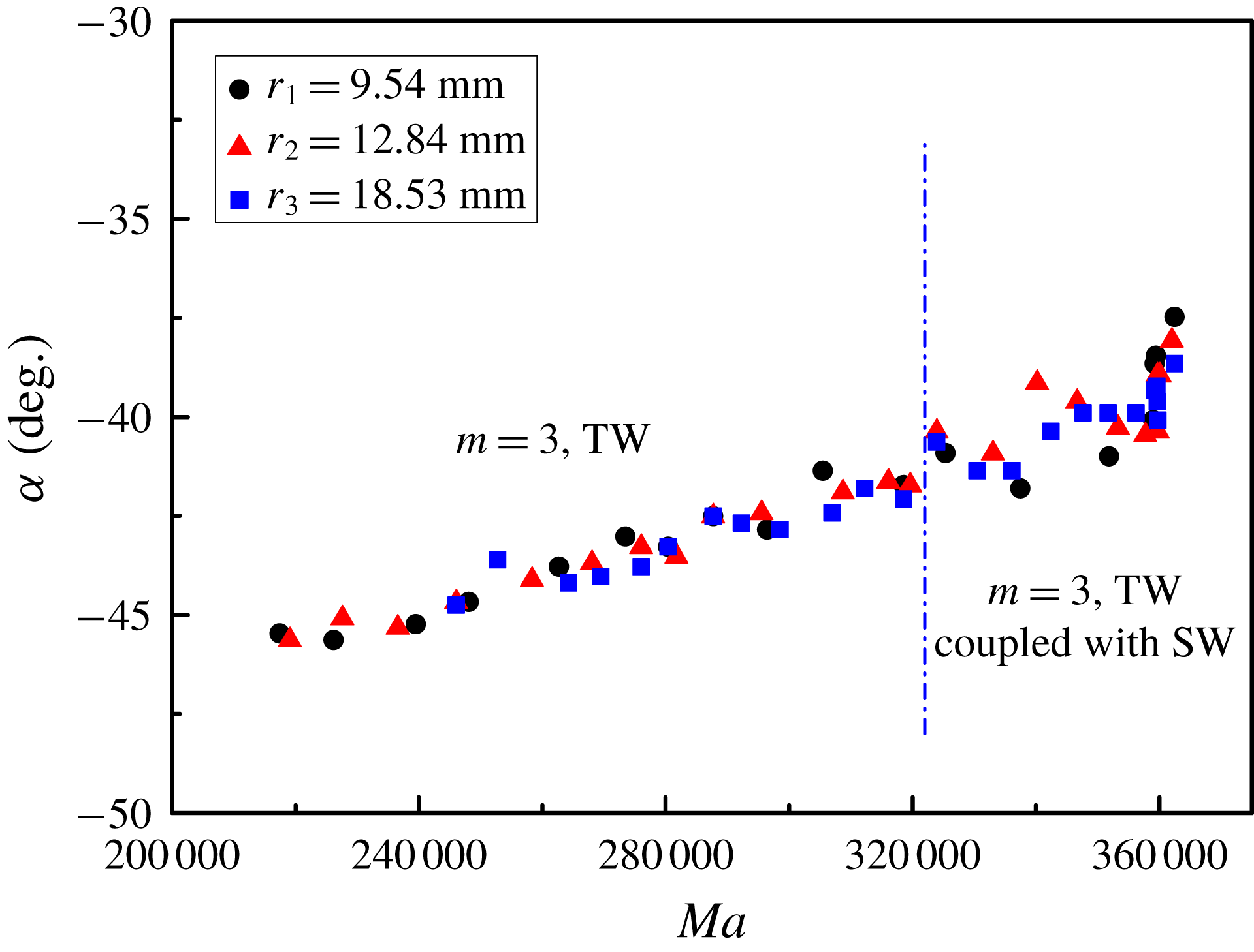
The propagation angle is the most intuitive characteristic of HTWs. It has been suggested in previous research that the propagation angle is independent of the Reynolds number. However, a different conclusion has been obtained in the present paper. The propagation angle can be presented as a function of the Marangoni number as shown in figure 14. Assuming counterclockwise is the positive direction, the propagation angle gradually decreases with increasing Ma. In other words, the tangent angle between the HTWs and the side walls becomes smaller and smaller. When the temperature field transits to the unique flow pattern that is coupled with the SW and the TW, there is no change in both the propagation direction and the angle of the HTWs, maintaining the previous flow characteristics. Three points in the same radial direction with different radii,
 $r_{1}<r_{2}<r_{3}$
(
 $r_{1}=9.54~\text{mm}$
,
 $r_{2}=12.84~\text{mm}$
,
 $r_{3}=18.53~\text{mm}$
), are selected to observe HTW propagation in the circumferential direction. As the radius – the distance from the inner wall – increases, the wave propagation angles,
 $\unicode[STIX]{x1D6FC}$
, are highly coincident with each other. It is evidenced that the isotherms connecting the inner and outer walls are straight lines.
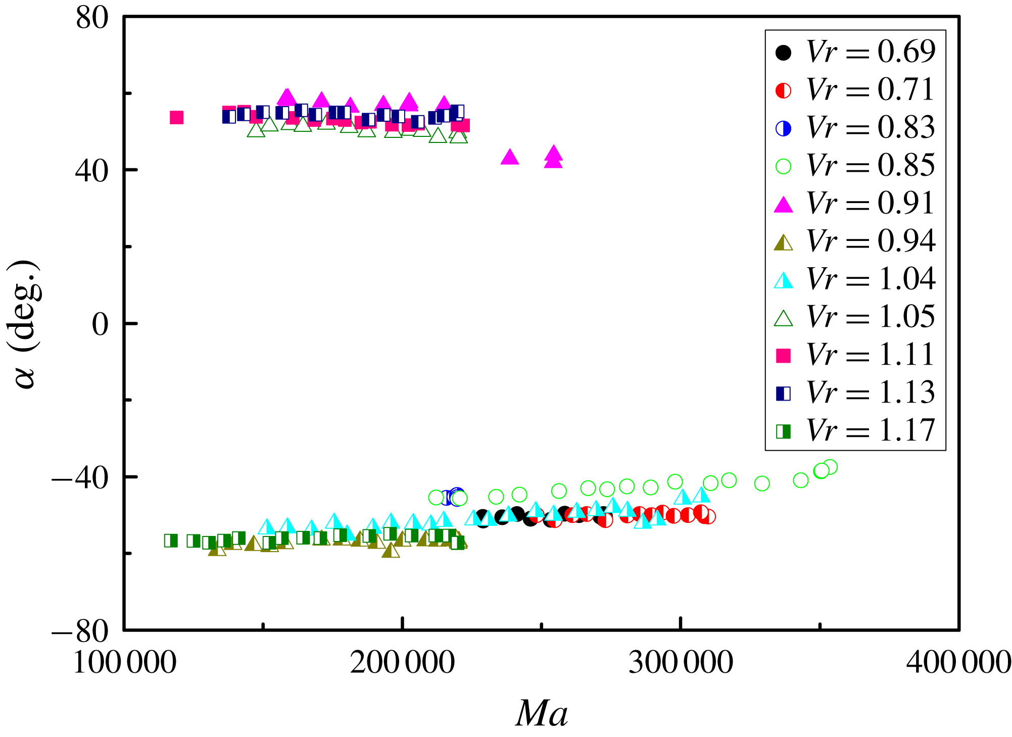
It is shown in figure 15 that
 $\unicode[STIX]{x1D6FC}$
can be influenced by Ma for given Vr, and the HTWs have inherent ‘inertia’ in propagation angle. The angles for the counterclockwise/clockwise propagation HTWs decrease notably at a rate of about
 $0.3^{\circ }$
per
 $^{\circ }\text{C}$
with increasing Ma, exhibiting excellent linear characteristics. When Ma increases from 12 000 to 35 000,
 $\unicode[STIX]{x1D6FC}$
changes from
 $55^{\circ }$
to
 $35^{\circ }$
. However, the volume ratio has no effect on the angles, which is contrary to the terrestrial results (Yu et al.
Reference Yu, Li, Wu and Chen2015). It may be that the flow field can be influenced by gravity, greatly determining the flow pattern transitions.
3.4 Amplitude and phase
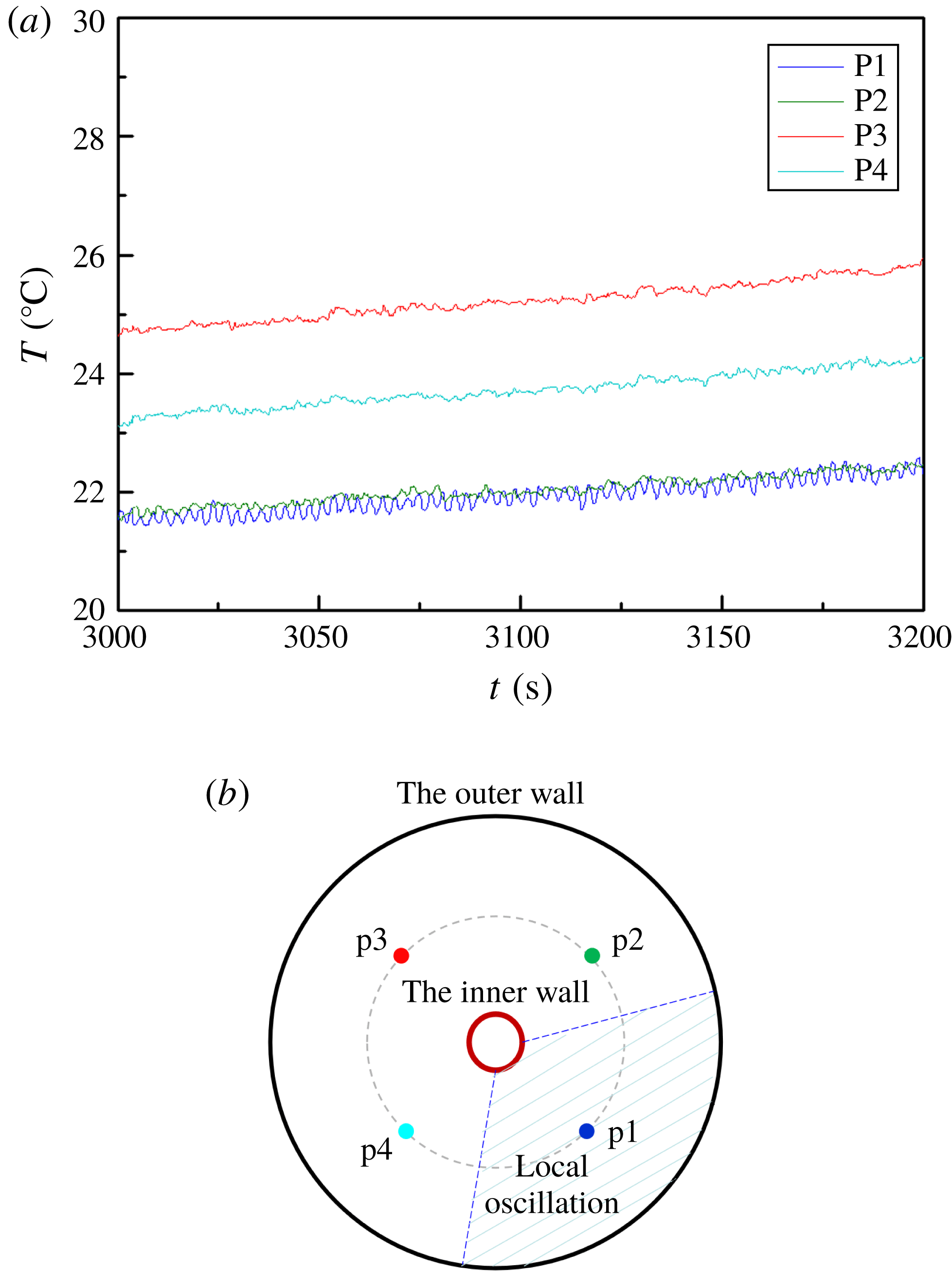
In addition to the flow patterns in the temperature field, the oscillation characteristics can be analysed by the temperature signals at certain points, which are extracted from the original infrared images. For
 $Vr<0.65$
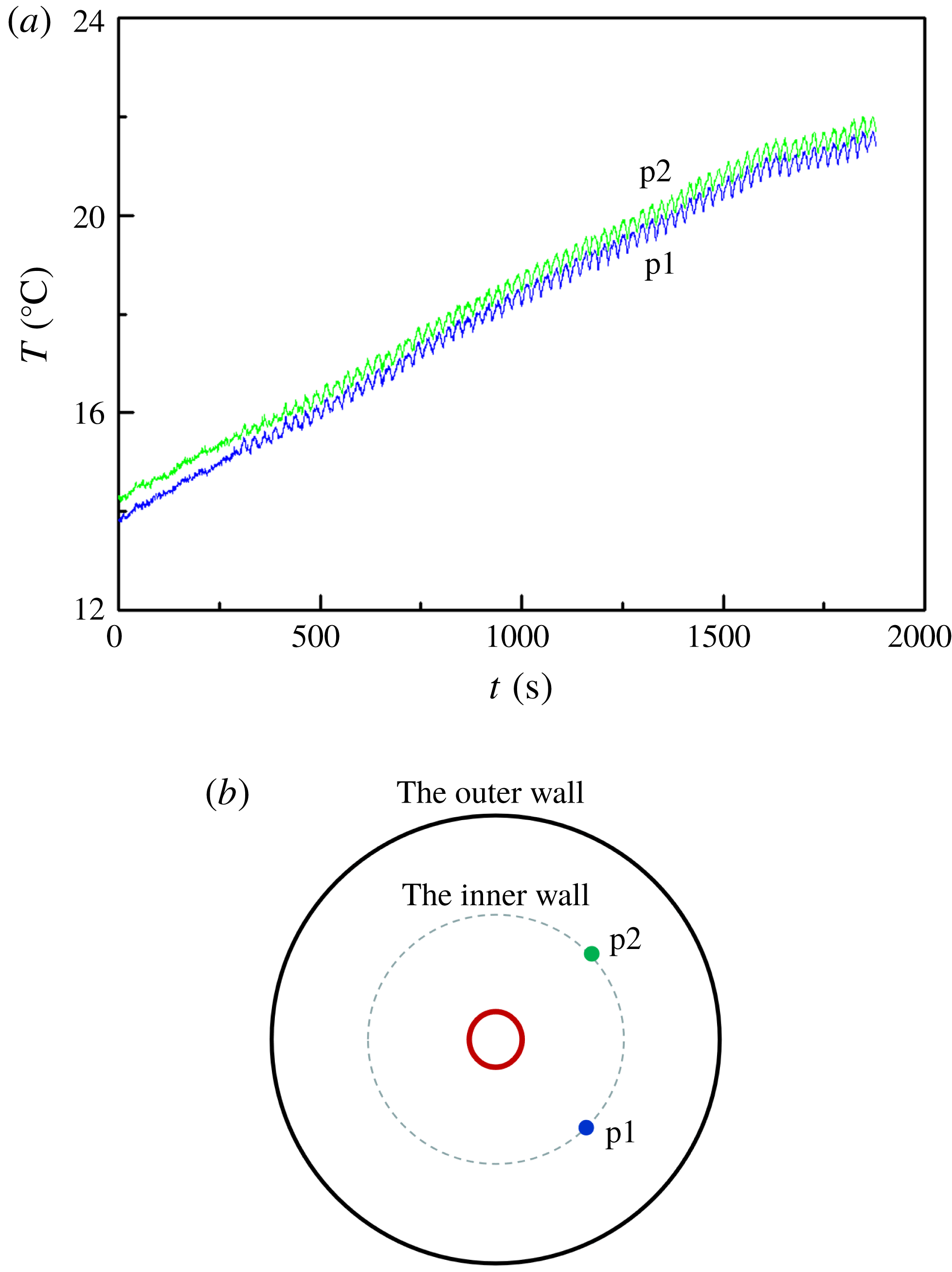
, the thin liquid layer limits the HTW development and influences the uniformity of the temperature distribution, which causes a difference in the temperature oscillation amplitude at different radial angles on the same circumference (figure 16). The temperature field enters into the local oscillation state. At point P1 the flow makes the periodic oscillation, while at other points the flow becomes disordered.
The circumferential temperature signal of the local oscillation for
 $Vr=0.42$
. (a) Temperature signals. (b) Point positions with a phase difference of
 $90^{\circ }$
.

The circumferential temperature signal of the regular oscillation. (a) Temperature signals. (b) Point positions with a phase difference of
 $90^{\circ }$
.

Variation of the circumferential temperature with temperature difference.

When
 $0.65<Vr$
, the oscillation temperature amplitude on the same circumference is equal for given
 $Ma$
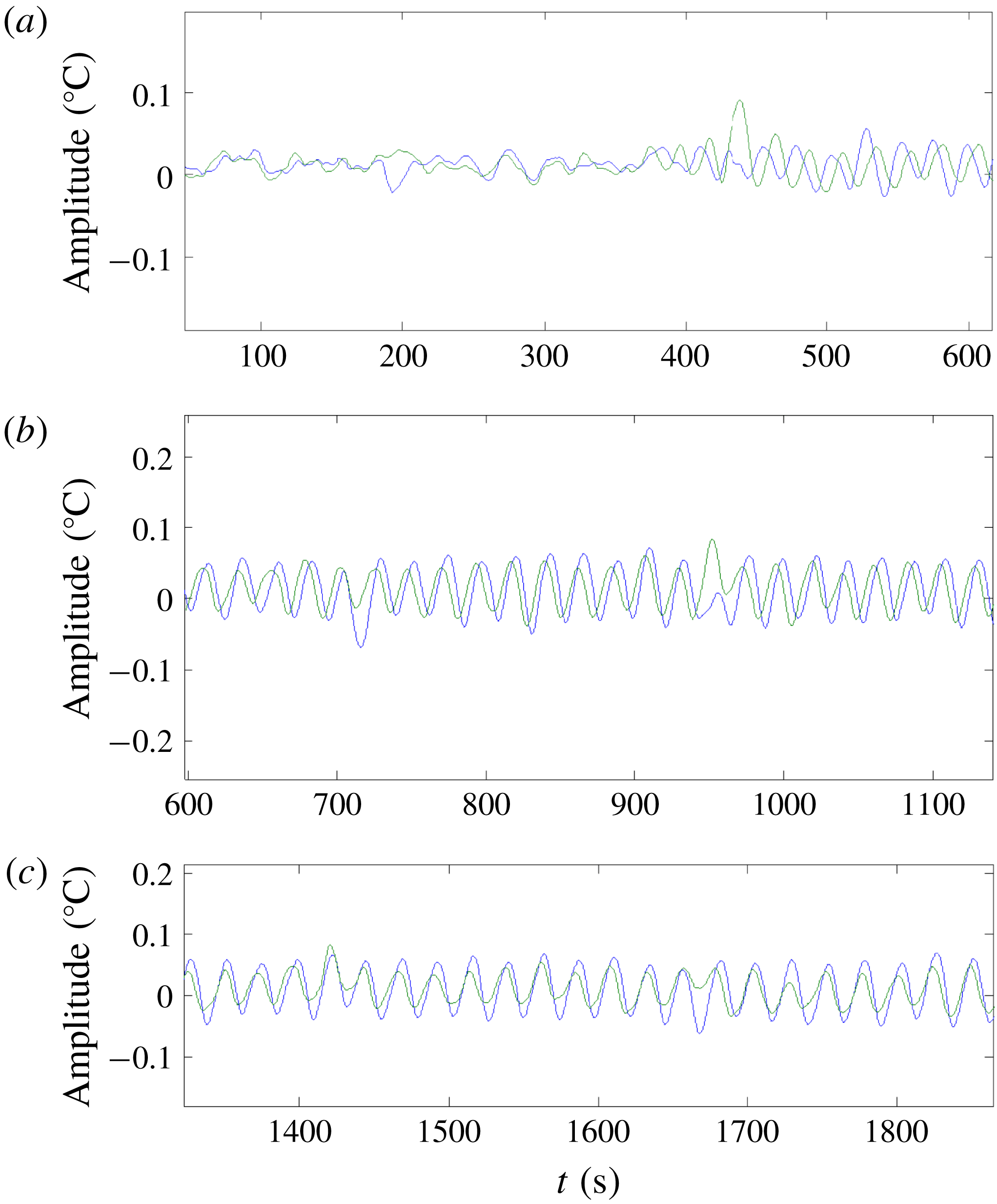
due to the symmetry of the annular LP. The flow pattern transition has led to the reconstruction of the flow field, which also can induce a change in the temperature phase difference for certain volume ratios.
The HTWs preserve the wavenumber unchanged when the temperature signals with a phase difference of
 $90^{\circ }$
lose their stability to oscillate simultaneously (figure 17). The temperatures change synchronously at these two points, their amplitudes increasing gradually as Ma increases. The phases at these two points remain stable and their phase difference is constant, as shown in figure 18.
As described above, the wavenumber can change with
 $0.83<Vr<0.91$
(figures 11 and 12). The oscillation phases in different radial directions are the same due to the flow field being axisymmetric at the beginning of the oscillation. But this state can be destroyed with increasing Ma, resulting in a change of phase.
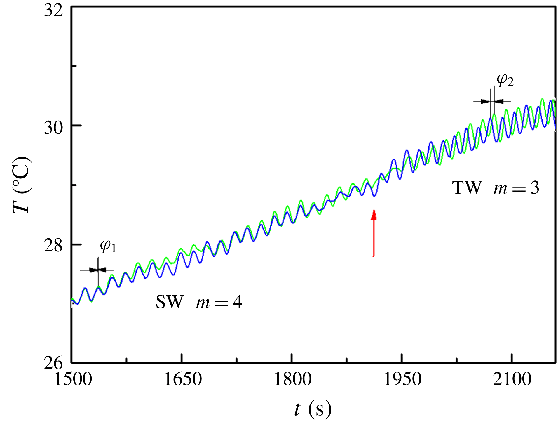
As shown in figure 19, in 1550–1850s, a SW motion with
 $m=4$
is caused by the initial symmetric perturbations introduced into the LP. The phase shift in the two azimuthal positions is constant, and their oscillatory amplitudes tend to be saturated. But in 1850–1950s, the SW motion appears to be unstable and then a transition process to the TW motion emerges. After a transition period, TW with
 $m=3$
(
 $t>1950\text{s}$
) can be observed for an extremely long duration, possessing a new constant phase shift. It is indicated that the flow pattern is sensitive to the temperature difference as the temperature difference has been only increased by
 $1.50\,^{\circ }\text{C}$
in this transition process.
Phase reversal occurs in the regular oscillation for
 $Vr=0.85$
(phase difference:
 $\unicode[STIX]{x1D711}_{1}=0$
,
 $\unicode[STIX]{x1D711}_{2}=0.76\unicode[STIX]{x03C0}$
).

3.5 Uncertainty analysis
Inevitable errors in experimental measurements can seriously affect the final experimental results. The uncertainty analysis method applied in this work is one of the most widely used error analysis methods. By this method, we can obtain the uncertainty in the experimental parameters. Based on previous work (Peng et al. Reference Peng, Li and Shi2007; Wu et al. Reference Wu, Guan, Xiao, Shen and Xu2013), neglecting errors caused by physical properties, the uncertainty of the Marangoni number can be simplified as follows:
 $$\begin{eqnarray}U_{Ma}=\left[\left(\frac{\unicode[STIX]{x2202}Ma}{\unicode[STIX]{x2202}T_{H}}U_{T_{H}}\right)^{2}+\left(\frac{\unicode[STIX]{x2202}Ma}{\unicode[STIX]{x2202}T_{L}}U_{T_{L}}\right)^{2}+\left(\frac{\unicode[STIX]{x2202}Ma}{\unicode[STIX]{x2202}R}U_{R}\right)^{2}+\left(\frac{\unicode[STIX]{x2202}Ma}{\unicode[STIX]{x2202}r}U_{r}\right)^{2}\right]^{1/2}.\end{eqnarray}$$
And the uncertainty of the volume ratio (Vr) caused by liquid injection/aspiration of liquid and radii of the annular pool is calculated as follows:
 $$\begin{eqnarray}U_{Vr}=\left[\left(\frac{\unicode[STIX]{x2202}Vr}{\unicode[STIX]{x2202}h}U_{h}\right)^{2}+\left(\frac{\unicode[STIX]{x2202}Vr}{\unicode[STIX]{x2202}r}U_{r}\right)^{2}+\left(\frac{\unicode[STIX]{x2202}Vr}{\unicode[STIX]{x2202}R}U_{R}\right)^{2}+\left(\frac{\unicode[STIX]{x2202}Vr}{\unicode[STIX]{x2202}d}U_{d}\right)^{2}\right]^{1/2},\end{eqnarray}$$
where
 $h$
is the distance realized by the PI motor injection/aspiration, and the minimum movement unit of the motor is
 $1~\text{count}=3.5\times 10^{-6}~\text{mm}$
.
It has been proved that 95 % of the standard random uncertainty regarding the readability can be characterized by half of the smallest scale division (Coleman & Steele Reference Coleman and Steele2009). For digital instruments, the smallest scale division is chosen as the instrument error. Therefore, the standard random uncertainties caused by temperature measurements and geometric dimensions of the LP are
 $0.05\,^{\circ }$
C and 0.01 mm, respectively.
According to equations (3.6) and (3.7), the synthetic standard uncertainty of Marangoni number in thermocapillary convection is determined to be 1.11 %. The uncertainty of volume ratio caused by factors including liquid evaporation and volume reading is within 4.00 %. Combined with uncertainties introduced by the liquid injection/aspiration and the geometry of the LP, the final synthetic uncertainty of the volume ratio is 4.07 %.
4 Conclusion
This paper reports the results of experiments regarding the instability of thermocapillary convection in an open annular LP carried out on the SJ-10 satellite. An overall analysis of the internal flow structure is of benefit for revealing the instability mechanism, studying the nonlinear characteristics and exploring the bifurcation transition of thermocapillary convection. The volume ratio effect on the critical conditions, the flow patterns and the transition processes of thermocapillary convection are researched in detail for the first time.
The temperature distribution on the liquid free surface has been measured with an infrared camera, and the flow pattern transition from the steady state to the oscillatory state is analysed. The flow structures can be categorized into three cases for different volume ratios, judging by the temperature distribution and the Fourier spectrum of the surface-temperature variation. (A) When the volume ratio is large, with increasing temperature difference, the flow field may transit gradually from the axisymmetric steady state to chaos. The non-uniformity of the temperature gradient distribution on the free surface tends to increase at a small temperature difference, which means the temperature gradient is larger on both the hot end and the cold end, while the temperature gradient in the middle is small. This non-uniform distribution introduces an initial perturbation into the internal flow, and generates the SW motion. As the SW state is not the stable solution for thermocapillary oscillatory flow, the external interference factor is expanded with further increasing temperature difference, and the flow field evolves into the TW state after the transition. The TW motion is a relatively stable state. Even though there could be small disturbances, the flow field can still maintain this flow state for a long duration. The increasing temperature difference initiated a novel oscillatory state in which the SW motion and the TW motion are coupled with each other. The temperature field also maintains its periodic structure in this oscillation regime. (B) In the case of very small volume ratio, the two-dimensional steady state transits directly into the local oscillatory flow once the temperature difference exceeds a threshold, with the coexistence of high-frequency oscillatory flow and steady-state flow. (C) When the volume ratio is relatively small, the boundary wall effect is obvious, and the regular periodic motion and the back flow influence each other, greatly disturbing the SW movement.
The effects of LP shape on the instability of thermocapillary convection are studied by changing the volume ratio, Vr, realized by injection/suction. The oscillatory data obtained from the LPs indicate that there is a significant effect of surface tension on the instability of the flow and the selection of the wavenumber. This is the first spatial verification for the nonlinear feature of the volume ratio in thermocapillary convection.
Some special properties of HTWs including the frequency and the wavenumber with large volume ratio are obtained owing to the microgravity environment. And these parameters are strongly determined by the temperature difference. As the temperature difference increases, the wavenumber shows a gradual decreasing trend, the frequency increases linearly and the propagation angle decreases linearly. The flow pattern transition causes the reconstruction of the flow field, resulting in the reversal of the phase.
In this paper, focusing on the volume ratio effect on thermocapillary convection, we perform an in-depth analysis of the infrared measurement results obtained on the SJ-10 satellite. Although there is indeed a certain distance from actual industrial production, it is meaningful for crystal growth, giving guidance and constructive opinions in theory. In fluid theory, the space experiment research of LPs is of great significance for the study of turbulence, and the development process of transition is clearer; this is difficult to observe in other flows. It is expected that the conclusions of this experiment can provide some useful reference for subsequent research of annular LPs or other related thermocapillary flow systems or even industrial production.
Acknowledgements
There are many participants who have contributed to the work reported. Besides the authors of the paper, P. Zhang, L. Duan, Z. Han and M. Hu in our team participated in the space experimental monitoring; L. Zhang and D. Zhang carried out the preliminary ground research on the thermocapillary convection experiment in the annular LP; Z. Jiang at Neusoft, Y. Yin, J. Yang, S. Zhao and S. Li at Astronauts Research and Training Center (ACC) participated in developing the space experimental equipment. Here we would like to express our great appreciation for all the work that has been accomplished by all participants. This project was funded by the Strategic Priority Research Program on Space Science of Chinese Academy of Sciences – SJ-10 Recoverable Scientific Experiment Satellite (XDA04020405 and XDA04020202-05) and the National Natural Science Foundation of China (U1738116). Q.K. and J.W. share first authorship for this paper.