1. Introduction
The rheological properties of a suspension are of great importance in the design process of many industries, such as food (Tabilo-Munizaga & Barbosa-Cánovas Reference Tabilo-Munizaga and Barbosa-Cánovas2005), pharmaceuticals (Nielloud Reference Nielloud2000) and oil (Ghanavati, Shojaei & Sa Reference Ghanavati, Shojaei and Ahmad2013). Other than conventional industrial applications, recent advances in various branches of biotechnology, such as blood rheology (MacMeccan et al. Reference MacMeccan, Clausen, Neitzel and Aidun2009; Omori et al. Reference Omori, Ishikawa, Imai and Yamaguchi2014), swimming of micro-organisms (Ishikawa & Pedley Reference Ishikawa and Pedley2007; Doostmohammadi, Stocker & Ardekani Reference Doostmohammadi, Stocker and Ardekani2012) and the dynamics of vesicles (Salac & Miksis Reference Salac and Miksis2012), have intensified research on suspensions.
Two forces associated with the dynamics of suspensions are the particle inertia and viscous flow (hydrodynamic) forces (Fall et al.
Reference Fall, Lemaître, Bertrand, Bonn and Ovarlez2010). The parameter that characterizes particle inertia relative to viscous effects is the Stokes number, which can be defined as
 $\mathit{St}=({\it\rho}_{p}/{\it\rho}_{f})\mathit{Re}$
, where
 ${\it\rho}_{p}$
and
 ${\it\rho}_{f}$
are the particle density and fluid density, respectively,
 $\mathit{Re}=\dot{{\it\gamma}}a^{2}/{\it\nu}$
is the particle Reynolds number,
 ${\it\nu}$
is the kinematic viscosity of the fluid,
 $a$
is the particle size, and
 $\dot{{\it\gamma}}$
is the shear rate of the flow (Haddadi & Morris Reference Haddadi and Morris2014). This parameter can be used to determine the crossover from the viscous to the inertial regime (Fall et al.
Reference Fall, Lemaître, Bertrand, Bonn and Ovarlez2010; Trulsson, Andreotti & Claudin Reference Trulsson, Andreotti and Claudin2012), and, depending on its value, a suspension can be categorized into three classes: Stokesian dynamics for a sufficiently small Stokes number, i.e. viscous forces are dominant (colloidal suspensions); suspensions with finite Stokes number; and granular suspensions, i.e. where particle inertia is dominant. The latter case refers to highly concentrated mixtures of solid particles (large enough to neglect the effect of Brownian motion and colloidal interactions) (Ancey, Coussot & Evesque Reference Ancey, Coussot and Evesque1999). At extreme concentrations close to the jamming transition, granular suspensions can even exhibit a divergence of their viscosity (Boyer, Guazzelli & Pouliquen Reference Boyer, Guazzelli and Pouliquen2011).
Considering the first two classes of suspensions, i.e. suspensions with negligible or finite Stokes number, rheological properties such as the viscosity are influenced by the presence of particles in a flow. By definition, the effective viscosity of a suspension is the viscosity of a homogeneous Newtonian fluid which provides the same shear stress when subjected to the same shear rate (Batchelor Reference Batchelor1970). The most important parameters affecting the rheology of suspensions are the particle volume fraction, the particle shape, interactions between particles, the spatial arrangement of particles within the suspension, and the nature of the bulk flow field (Jeffrey & Acrivos Reference Jeffrey and Acrivos1976; Mueller, Llewellin & Mader Reference Mueller, Llewellin and Mader2010). The dominant parameter affecting the effective viscosity is the volume fraction of the suspension
 ${\it\phi}$
(volume occupied by particles per unit volume of the suspension). For sufficiently low particle concentrations, the relative viscosity (effective viscosity of the suspension normalized by the viscosity of the fluid) as a function of volume fraction can be approximated by the following series (a-Holek & Mendoza Reference a-Holek and Mendoza2010):
 $$\begin{eqnarray}{\it\eta}_{r}=1+[{\it\eta}]{\it\phi}+k_{H}{\it\phi}^{2}+\cdots \,,\end{eqnarray}$$
where
 $[{\it\eta}]$
and
 $k_{H}$
are the intrinsic viscosity and the Huggins coefficient, respectively. The second-order term
 $k_{H}{\it\phi}^{2}$
is considered when particle interactions need to be included in the calculation (Batchelor & Green Reference Batchelor and Green1972), while the intrinsic viscosity
 $[{\it\eta}]$
conveys the particle contribution to the relative viscosity in dilute regimes. Einstein (Reference Einstein1906) was the first to estimate the intrinsic viscosity of a dilute suspension consisting of rigid spheres (
 $[{\it\eta}]=2.5$
) by calculating the rate of energy dissipation in the suspension. Jeffery (Reference Jeffery1922) extended Einstein’s results to ellipsoids, and analytically computed the intrinsic viscosity for ellipsoids with different ellipticities and orientations. Batchelor (Reference Batchelor1970) established an averaging procedure to obtain the average properties of the solution from the suspended particles. Batchelor & Green (Reference Batchelor and Green1972) used the averaging procedure of Batchelor (Reference Batchelor1970) and calculated the Huggins coefficient for a suspension of spherical particles, taking into consideration particle interactions.
The intrinsic viscosity – and consequently the solution viscosity – depend on the shape, size and concentration, i.e. the microstructure of the colloidal particles (Jeffrey & Acrivos Reference Jeffrey and Acrivos1976). Therefore, many theoretical models have been proposed based on different particle shapes and assumptions, e.g. see Jeffery (Reference Jeffery1922), Huggins (Reference Huggins1942), Eilers (Reference Eilers1949), Mooney (Reference Mooney1951) and Pal & Rhodes (Reference Pal and Rhodes1989), among others. Although such analytical models have shed light on many aspects of the rheology of suspensions, they inherently face some limitations. The first limitation is that the Stokes equations, used in the analytical models, are the result of neglecting the inertia of the flow. Therefore, analytical solutions are mainly applicable at the
 $\mathit{Re}\rightarrow 0$
limit (Rallison Reference Rallison1978; Lipscomb et al.
Reference Lipscomb, Denn, Hur and Boger1988; Berlyand, Borcea & Panchenko Reference Berlyand, Borcea and Panchenko2005; Subramanian et al.
Reference Subramanian, Koch, Zhang and Yang2011). For suspensions with finite Reynolds numbers, the analytical approaches typically use perturbation expansions to the Stokes solution (Lin, Peery & Schowalter Reference Lin, Peery and Schowalter1970; Subramanian et al.
Reference Subramanian, Koch, Zhang and Yang2011). However, the experimental study of Poe & Acrivos (Reference Poe and Acrivos1975) later showed that the solutions of Lin et al. (Reference Lin, Peery and Schowalter1970) are valid for very low Reynolds numbers (
 $\mathit{Re}<0.1$
), and are not accurate for moderate inertial regimes.
Another limitation of the analytical approach is that it is only applicable to simple particle shapes such as spheres (Ryskin, Ryskin & Rallison Reference Ryskin, Ryskin and Rallison1980; Wilson & Davis Reference Wilson and Davis2000), ellipsoids (Jeffery Reference Jeffery1922; Claeys & Brady Reference Claeys and Brady1993), or other axisymmetric particles (Hinch & Leal Reference Hinch and Leal1972; Brenner Reference Brenner1974; Haber & Brenner Reference Haber and Brenner1984). Furthermore, even for very low Reynolds numbers and simple geometries, the Stokesian dynamics may require numerical techniques to study the microstructure of a suspension or calculate the rheological parameters when particle interactions become significant in a dense suspension (Meng & Higdon Reference Meng and Higdon2008; Kumar & Higdon Reference Kumar and Higdon2011a ,Reference Kumar and Higdon b ).
The development of fluid–structure interaction (FSI) methods has enabled us to simulate suspension problems without neglecting particle motion and Brownian effects. In FSI algorithms, sometimes referred to as hybrid methods (MacMeccan et al.
Reference MacMeccan, Clausen, Neitzel and Aidun2009; Clausen & Aidun Reference Clausen and Aidun2010), a flow solver is used to calculate the fluid force (torque) exerted on the particles immersed in the fluid. This solver is coupled to a structure solver to compute particle motion by solving the Newtonian dynamics for rigid particles, or displacements for deformable particles. Mikulencak & Morris (Reference Mikulencak and Morris2004) computed the flow around both fixed and torque-free spheres in a simple shear flow in the range
 $0<\mathit{Re}\leqslant 100$
using finite element methods. Applying the lattice–Boltzmann method (LBM), Verberg & Koch (Reference Verberg and Koch2006) performed three-dimensional simulations of particles heavier than the fluid in a wall-bounded linear shear flow to study the effects of both fluid and particle inertia on the suspension rheology. Kulkarni & Morris (Reference Kulkarni and Morris2008) studied neutrally buoyant particles in a wall-bounded shear flow, and investigated the bulk rheological properties (relative viscosity, normal stress differences and particle pressure) for
 $0.01\leqslant \mathit{Re}\leqslant 5$
. MacMeccan et al. (Reference MacMeccan, Clausen, Neitzel and Aidun2009) developed a model to simulate suspensions of deformable particles by coupling the LBM for the fluid phase to a linear finite element analysis (FEA) describing particle deformation. Implementing the model, they simulated suspensions of hundreds of biconcave red blood cells at 40 % volume fraction and predicted the suspension viscosity and the shear-thinning behaviour of blood. Using the same (LBM/FEA) model, Clausen & Aidun (Reference Clausen and Aidun2010) studied the influence of capsule dynamics on the rheology of a capsule suspension. They studied initially spherical capsules undergoing a tank-treading behaviour and assumed an ellipsoidal shape at a steady orientation while the capsule membrane rotated. Other numerical approaches such as the level-set method are widely used, especially in the field of vesicle (biological particles with a lipid layer forming a membrane between internal and external fluids) microstructures and rheology. Salac & Miksis (Reference Salac and Miksis2012) investigated the influence of inertia on the dynamical modes of a vesicle (tumbling and tank-treading) in a shearing flow in two dimensions. They observed that, as the Reynolds number increased, the maximum tension on the vesicle membrane also increased. Recently, using the Force Coupling Method in periodic computational domains, Yeo & Maxey (Reference Yeo and Maxey2013) studied the rheology and particle-scale dynamics of concentrated suspensions consisting of neutrally buoyant particles in a homogeneous linear shear flow for the range of Reynolds number
 $0.005\leqslant \mathit{Re}\leqslant 2$
. Nevertheless, the role of inertia in the rheology of a suspension has not been the focus of any of the aforementioned studies.
Experimental studies of suspensions, from very dilute to highly concentrated, have been used to derive valuable empirical correlations for the constitutive laws of rheology. However, they are not capable of identifying the mechanisms by which particles contribute to the rheological parameters because measuring the stresses on the particles using experimental techniques is quite challenging, if not impossible (Stover, Koch & Cohen Reference Stover, Koch and Cohen1992; Zarraga, Hill & Leighton Jr Reference Zarraga, Hill and Leighton2000; Zettner & Yoda Reference Zettner and Yoda2001; Singh & Nott Reference Singh and Nott2003; Stickel & Powell Reference Stickel and Powell2005). The physics of rheology and the mechanism of stress generation by particles are best described by numerical or theoretical work. The theoretical framework outlined by Batchelor (Reference Batchelor1970) to analyse the different mechanisms of stress in a suspension is still regularly used in the majority of numerical studies. Based on this approach, the bulk stress of a suspension is increased due to the presence of particles by an amount known as the ‘particle stress’, which is generated by the stresslet (dipole force strength of the particle) along with the acceleration and the Reynolds stress.
Numerical simulations of suspensions have clarified many aspects of the stress generation mechanisms (stresslet, acceleration stress, and Reynolds stress). However, most of the previous numerical simulations have been limited to suspensions of spherical particles: Verberg & Koch (Reference Verberg and Koch2006) considered the Reynolds stress contribution for spherical particles without discussing the acceleration stress term; Kulkarni & Morris (Reference Kulkarni and Morris2008) calculated all terms of the particle stress and found the effect of the acceleration stress and the Reynolds stress to be almost negligible; Haddadi & Morris (Reference Haddadi and Morris2014) investigated the contributions of different terms of the particle stress up to
 $\mathit{Re}\sim O(5)$
and found the magnitude of the second normal stress difference generated by the Reynolds stress is non-negligible when
 $\mathit{Re}\geqslant 1$
.
On the other hand, research on non-spherical particles has been restricted mainly to experimental studies (Metzger, Guazzelli & Butler Reference Metzger, Guazzelli and Butler2005; Pabst, Gregorová & Berthold Reference Pabst, Gregorová and Berthold2006; Gunes et al. Reference Gunes, Scirocco, Mewis and Vermant2008; Mueller et al. Reference Mueller, Llewellin and Mader2010; Cheng et al. Reference Cheng, McCoy, Israelachvili and Cohen2011), Stokesian modelling (Hinch & Leal Reference Hinch and Leal1972; Claeys & Brady Reference Claeys and Brady1993; Ausias, Fan & Tanner Reference Ausias, Fan and Tanner2006; Kumar & Higdon Reference Kumar and Higdon2011a ,Reference Kumar and Higdon b ), or simulations that ignore acceleration and Reynolds stress mechanisms (Ross & Klingenberg Reference Ross and Klingenberg1997; Lindström & Uesaka Reference Lindström and Uesaka2009; MacMeccan et al. Reference MacMeccan, Clausen, Neitzel and Aidun2009; Clausen & Aidun Reference Clausen and Aidun2010; Wu & Aidun Reference Wu and Aidun2010). Therefore, the role of inertia in the physics of suspensions of non-spherical particles has yet to be fully understood.
In this work, we calculate rheological parameters such as the components of the particle stress, the effective viscosity of the suspension, and the kinematics of particle motion using both numerical and analytical methods. By comparing analytical and numerical solutions, we verify our numerical results (at low
 $\mathit{Re}$
) and identify the effects of inertia at different Reynolds numbers. We have investigated the influence of inertia on all mechanisms of particle stress, to the best of the authors’ knowledge, for the first time for a suspension of prolate ellipsoidal particles. Although the framework is capable of handling any complex-shaped particle, we have concentrated on ellipsoidal particles because analytical solutions are available for ellipsoids (assuming the Stokes problem for a single particle). Therefore, we are able to discuss the effect of inertia on each particle stress mechanism by comparing numerical results with the corresponding analytical solution, which ignores inertia. We find that almost all rheological parameters of suspensions are influenced by the inertia, as will be discussed in §§ 4 and 5. This paper is organized as follows: in § 2 we will briefly discuss the structure solver, 3-D rigid body rotation, the flow solver, the FSI coupling technique, and the formulation used to calculate the particle stress and relative viscosity. In § 3 we discuss the motion of prolate ellipsoids under simple shear for various aspect ratios, and compare our results with the Stokesian solution of Jeffery (Reference Jeffery1922) at different Reynolds numbers. We report the particle stress tensor for the smallest physical time scale (as functions of orientation) for prolate ellipsoidal particles and compare numerical results with the analytical solutions in § 4. In this section, we also discuss the role of the particle Reynolds number, particle shape and volume fraction on different mechanisms of the particle stress. In § 5 the cycle-average intrinsic viscosity and normal stress differences of the suspensions are calculated and the influence of inertia (
 $\mathit{Re}$
), shape (
 $\mathit{Ar}$
) and volume fraction (
 ${\it\phi}$
) on them are compared. Finally, we will summarize the findings of this work in § 6. In addition, analytical solutions for the stresslet, acceleration and Reynolds stress tensors, which are used to validate the numerical results, are provided in the appendices.
2. Method and material
The numerical method used to simulate the motion of neutrally buoyant particles in the shear flow is the curvilinear immersed-boundary (CURVIB) method (Gilmanov & Sotiropoulos Reference Gilmanov and Sotiropoulos2005; Ge & Sotiropoulos Reference Ge and Sotiropoulos2007; Borazjani, Ge & Sotiropoulos Reference Borazjani, Ge and Sotiropoulos2008) coupled with the rigid body dynamics of moving particles. We have used the quaternion–angular velocity equations, instead of a conventional rotation matrix, to find the instantaneous orientation of the particle in order to avoid numerical drift. These solvers are coupled together through a strong-coupling with under-relaxation approach (Borazjani et al. Reference Borazjani, Ge and Sotiropoulos2008). Details of the computational method and the FSI can be found in previous publications (Gilmanov & Sotiropoulos Reference Gilmanov and Sotiropoulos2005; Ge & Sotiropoulos Reference Ge and Sotiropoulos2007; Borazjani et al. Reference Borazjani, Ge and Sotiropoulos2008, Reference Borazjani, Ge, Le and Sotiropoulos2013; Borazjani Reference Borazjani2013a ), and only a brief overview is provided in what follows.
2.1. Structure solver and 3-D rigid body rotation equations
The surface of any arbitrarily shaped particle,
 ${\it\Gamma}(t)$
, is discretized with an unstructured triangular mesh, forming a list of
 $K$
material points. These points can be tracked over time by their global Lagrangian position vector
 $\boldsymbol{r}^{k}(t)$
(
 $k=1,K$
):
 $$\begin{eqnarray}\boldsymbol{r}^{k}(t)\in {\it\Gamma}(t),\quad \forall t>0,\quad \boldsymbol{r}^{k}(0)=\boldsymbol{r}_{0}^{k},\end{eqnarray}$$
where
 $\boldsymbol{r}_{0}^{k}$
is the initial location of the
 $k\text{th}$
material point on
 ${\it\Gamma}(0)$
. The particle rotates in the background fluid due to the torque exerted by flow. The rotation matrix which describes such rotation in three-dimensional space is denoted as
 $\unicode[STIX]{x1D64D}$
. First, we define the shape of the rigid body in terms of a coordinate reference system attached to the body at its centre of mass (this coordinate system rotates with the same angular velocity as the rigid body and is referred to as the body frame). Therefore, the position vector of the material point
 $k$
remains unchanged over time in this reference frame. Having the geometric description of the rigid body in the body frame, we use
 $\unicode[STIX]{x1D64D}(t)$
to transform the body-frame description into the inertial frame and find the instantaneous position vector of point
 $k$
in the inertial coordinate system as:
 $$\begin{eqnarray}\boldsymbol{r}^{k}(t)=\unicode[STIX]{x1D64D}(t)(\boldsymbol{r}_{0}^{k}-\boldsymbol{r}_{c})+\boldsymbol{r}_{c},\end{eqnarray}$$
where
 $\boldsymbol{r}_{c}$
is the position vector of the particle’s centre of mass and
 $\boldsymbol{r}_{0}^{k}$
is the position vector of point
 $k$
expressed in the body space, i.e. the position vector of the same point in the global frame at the beginning of the motion. Equation (2.2) reveals that we need to compute the rotation matrix at each specific time in order to define the orientation of the body. To do so, we should solve the dynamic equation of motion for the particle while it moves in the fluid. Motion of the immersed body in the fluid results in a hydrodynamic reacting force (torque) exerted on the surface of the body. The total external torque is defined as:
 $$\begin{eqnarray}\boldsymbol{M}(t)=\mathop{\sum }_{k}\boldsymbol{M}_{k}(t)=\mathop{\sum }_{k}[\boldsymbol{r}_{k}(t)-\boldsymbol{r}_{c}(t)]\times \boldsymbol{F}_{k}(t),\end{eqnarray}$$
where
 $\boldsymbol{F}_{k}(t)$
denotes the total force from the fluid acting on the
 $k\text{th}$
point at time
 $t$
. Knowing the total hydrodynamic torque exerted on the body, we can compute the angular momentum of the body by integrating the following equation:
 $$\begin{eqnarray}\frac{\text{d}\boldsymbol{L}(t)}{\text{d}t}=\boldsymbol{M}(t),\end{eqnarray}$$
where
 $\boldsymbol{L}$
is the angular momentum of the body defined as:
 $$\begin{eqnarray}\boldsymbol{L}(t)=\unicode[STIX]{x1D644}(t){\bf\omega}(t),\end{eqnarray}$$
where
 $\unicode[STIX]{x1D644}$
and
 ${\bf\omega}$
are the instantaneous moment of inertia matrix and the angular velocity vector, respectively. In addition,
 $\unicode[STIX]{x1D644}(t)$
depends on the orientation of the body, and we can find the moment of inertia tensor in terms of the constant-value moment of inertia computed in the body reference frame and the rotation matrix as:
 $$\begin{eqnarray}\unicode[STIX]{x1D644}(t)=\unicode[STIX]{x1D64D}(t)\unicode[STIX]{x1D644}_{b}\unicode[STIX]{x1D64D}^{\text{T}}(t),\end{eqnarray}$$
where
 $\unicode[STIX]{x1D644}_{b}$
is calculated with respect to the body-frame coordinate system and remains constant over the simulation. Considering (2.4)–(2.6), it is clear that we need one more equation to solve for all the unknown variables, including
 $\boldsymbol{L}(t)$
,
 $\unicode[STIX]{x1D644}(t)$
,
 ${\bf\omega}(t)$
and
 $\unicode[STIX]{x1D64D}(t)$
. The final equation to close the system of differential equations and fully determine the dynamics of rigid body rotation is the time evolution of the rotation matrix due to the angular velocity of the body. Instead of the conventional method of solving for
 $\unicode[STIX]{x1D64D}(t)$
, it is preferable to use quaternions,
 $\boldsymbol{q}(t)$
, to represent the orientation of the body in three-dimensional space (Shoemake Reference Shoemake1985; Baraff Reference Baraff1997; Kuipers Reference Kuipers1999) to avoid the numerical drift. Since we still need the rotation matrix to calculate the moment of inertia, i.e. (2.6),
 $\unicode[STIX]{x1D64D}(t)$
will be computed as an auxiliary variable from
 $\boldsymbol{q}(t)$
as follows:
 $$\begin{eqnarray}\unicode[STIX]{x1D64D}=\left[\begin{array}{@{}ccc@{}}1-2q_{2}^{2}-2q_{3}^{2} & 2(q_{1}q_{2}-q_{0}q_{3}) & 2(q_{1}q_{3}+q_{0}q_{2})\\ 2(q_{1}q_{2}+q_{0}q_{3}) & 1-2q_{1}^{2}-2q_{3}^{2} & 2(q_{2}q_{3}-q_{0}q_{1})\\ 2(q_{1}q_{3}-q_{0}q_{2}) & 2(q_{2}q_{3}+q_{0}q_{1}) & 1-2q_{1}^{2}-2q_{2}^{2}\end{array}\right].\end{eqnarray}$$
We also need the following equation to calculate the quaternion vector during the simulation:
 $$\begin{eqnarray}\frac{\text{d}\boldsymbol{q}}{\text{d}t}=\frac{1}{2}\boldsymbol{q}\times {\bf\omega}=\frac{1}{2}\left[\begin{array}{@{}cccc@{}}0 & -{\it\omega}_{1} & -{\it\omega}_{2} & -{\it\omega}_{3}\\ {\it\omega}_{1} & 0 & -{\it\omega}_{3} & {\it\omega}_{2}\\ {\it\omega}_{2} & {\it\omega}_{3} & 0 & -{\it\omega}_{1}\\ {\it\omega}_{3} & -{\it\omega}_{2} & {\it\omega}_{1} & 0\end{array}\right]\left[\begin{array}{@{}c@{}}q_{1}\\ q_{2}\\ q_{3}\\ q_{4}\end{array}\right].\end{eqnarray}$$
Now we have enough equations ((2.4)–(2.8)) to close the system of equations and solve for all the unknown variables of the particle dynamics
 $(\boldsymbol{L},\unicode[STIX]{x1D644},{\bf\omega},\unicode[STIX]{x1D64D},\boldsymbol{q})$
.
2.2. Flow solver
The equations governing the motion of an incompressible Newtonian viscous fluid are the unsteady 3-D Navier–Stokes equations. Non-dimensionalized by a characteristic velocity
 $\dot{{\it\gamma}}a$
and the particle radius
 $a$
, the governing equations in curvilinear coordinates read as follows:
 $$\begin{eqnarray}\displaystyle & \displaystyle J\frac{\partial \mathfrak{U}^{r}}{\partial {\it\xi}^{r}}=0, & \displaystyle\end{eqnarray}$$
 $$\begin{eqnarray}\displaystyle & \displaystyle \frac{\partial \mathfrak{U}^{r}}{\partial t}=\frac{{\it\xi}_{q}^{r}}{J}\left[-J\frac{\partial }{\partial {\it\xi}^{p}}(\mathfrak{U}^{p}u_{q})-J\frac{\partial }{\partial {\it\xi}^{p}}\left(\frac{{\it\xi}_{q}^{p}}{J}p\right)+\frac{1}{\mathit{Re}}J\frac{\partial }{\partial {\it\xi}^{p}}\left(\frac{g^{pm}}{J}\frac{\partial u_{q}}{\partial {\it\xi}^{m}}\right)\right], & \displaystyle\end{eqnarray}$$
 $$\begin{eqnarray}\displaystyle & \displaystyle \mathit{Re}=\frac{\dot{{\it\gamma}}a^{2}}{{\it\nu}}, & \displaystyle\end{eqnarray}$$
 $J$
is the determinant of the Jacobian of the transformation,
 ${\it\xi}_{q}^{r}=\partial {\it\xi}^{r}/\partial x_{q}$
,
 $g^{rm}={\it\xi}_{q}^{r}{\it\xi}_{q}^{m}$
are the contravariant metrics of the transformation,
 $\mathfrak{U}^{r}=u_{m}{\it\xi}_{m}^{r}/J$
is the contravariant volume flow rate,
 $u_{q}$
is the non-dimensional Cartesian velocity of the fluid,
 $p$
is the pressure non-dimensionalized by
 ${\it\rho}\dot{{\it\gamma}}^{2}a^{2}$
and
 $a$
is one-half the largest diameter of the particle.
Equations (2.9) are solved over curvilinear grids using a hybrid staggered/non-staggered discretization with the QUICK (Quadratic Upstream Interpolation for Convective Kinematics) scheme for the convective terms and the central difference for the viscous terms. The equations are integrated in time using an efficient, second-order-accurate fractional step methodology with a Newton–Krylov solver for the momentum equations, and a Generalized Minimal Residual Method (GMRES) solver enhanced with multigrid as a preconditioner for the Poisson equation (Ge & Sotiropoulos Reference Ge and Sotiropoulos2007; Borazjani et al. Reference Borazjani, Ge and Sotiropoulos2008). The code is parallelized using Message Passing Interface (MPI) and the parallel libraries of PETSc (Portable, Extensible Toolkit for Scientific Computation) (Balay et al. Reference Balay, Abhyankar, Adams, Brown, Brune, Buschelman, Dalcin, Eijkhout, Gropp, Kaushik, Knepley, McInnes, Rupp, Smith, Zampini and Zhang2001) to efficiently utilize the supercomputing facilities available to the authors.
To handle the moving boundaries, a sharp-interface immersed-boundary method is used (Gilmanov & Sotiropoulos Reference Gilmanov and Sotiropoulos2005; Ge & Sotiropoulos Reference Ge and Sotiropoulos2007; Borazjani et al. Reference Borazjani, Ge and Sotiropoulos2008). In this method, the fluid grid is fixed and does not move with the boundary, making it more suitable for large deformations because it does not create highly skewed grids. The sharp interface is maintained by reconstructing the boundary conditions at the nodes that are exterior to, but adjacent to the immersed-boundary surface using interpolation along the local normal to the boundary, as has been shown to be second-order accurate (Gilmanov & Sotiropoulos Reference Gilmanov and Sotiropoulos2005). The background nodes at each time step are classified into fluid, wall and immersed-boundary nodes using an efficient ray-tracing algorithm described in detail in Borazjani et al. (Reference Borazjani, Ge and Sotiropoulos2008). The method has been fully validated and applied to a wide range of problems, including cardiovascular flows (Borazjani, Ge & Sotiropoulos Reference Borazjani, Ge and Sotiropoulos2010a ; Borazjani & Sotiropoulos Reference Borazjani and Sotiropoulos2010a ; Borazjani Reference Borazjani2013a ), aquatic swimming (Borazjani et al. Reference Borazjani, Sotiropoulos, Malkiel and Katz2010c ; Borazjani & Sotiropoulos Reference Borazjani and Sotiropoulos2010b ; Borazjani Reference Borazjani2013b ; Borazjani & Daghooghi Reference Borazjani and Daghooghi2013), and vortex-induced vibrations (Borazjani & Sotiropoulos Reference Borazjani and Sotiropoulos2009).
2.3. Coupling methods for partitioned FSI problems
The structure domain is coupled to the fluid domain through the dynamic boundary condition (2.4), i.e. the torque on the right-hand side of the equation is a function of fluid variables (velocity and pressure). In addition, the fluid domain is coupled to the structure domain through the no-slip boundary condition on the immersed boundaries. Using the strong-coupling partitioned approach with under-relaxation (Borazjani et al. Reference Borazjani, Ge and Sotiropoulos2008), we solve the fluid and structured domain together. In this method, the fluid and structure domains are separately advanced in time, but the simultaneous (implicit) solution of both equations is achieved through fluid/structure sub-iterations. The strong-coupling scheme is computationally expensive since each sub-iteration requires the solution of both structural and fluid equations. However, due to its stabilizing capability, implementing strong coupling enables us to choose time steps up to 20 times larger than with loose coupling.
2.4. Formulation of rheological parameters
The last step in our numerical framework is the calculation of the particle stress from the simulated motion of fluid and particles. We implemented the approach developed by Batchelor (Reference Batchelor1970) to compute the bulk stress generated by a flowing suspension in terms of volume averages. The volume-averaged stress (non-dimensionalized by
 ${\it\rho}\dot{{\it\gamma}}^{2}a^{2}$
) in a statistically homogenous suspension is calculated as:
 $$\begin{eqnarray}{\it\Sigma}_{ij}=-{\it\delta}_{ij}\frac{1}{V}\int _{V_{f}}p\,\text{d}V+{\it\mu}\left(\frac{\partial \mathscr{U}_{i}}{\partial x_{j}}+\frac{\partial \mathscr{U}_{j}}{\partial x_{i}}\right)+{\it\Sigma}_{ij}^{p},\end{eqnarray}$$
where
 $V_{f}$
is the volume occupied by the fluid and
 $\partial \mathscr{U}_{i}/\partial x_{j}$
is the volume-averaged velocity gradient. The quantity
 ${\it\Sigma}_{ij}^{p}$
, named the ‘particle stress’ by Batchelor (Reference Batchelor1970), represents the contribution to the bulk stress due to the presence of particles. For rigid particles, this contribution reads as follows:
 $$\begin{eqnarray}{\it\Sigma}_{ij}^{p}=\frac{1}{V}\mathop{\sum }_{n=1}^{N}\int _{(V_{p})_{n}}{\it\sigma}_{ij}\,\text{d}V-\frac{1}{V}\int _{V}({\it\rho}u_{i}^{\prime }u_{j}^{\prime })\,\text{d}V,\end{eqnarray}$$
where
 $V_{p}$
is the particle volume,
 $N$
is the total number of particles in the suspension,
 ${\it\sigma}_{ij}$
is the Newtonian stress, and
 $u_{i}^{\prime }$
are velocity fluctuations. As is evident in (2.11), particle stress is generated by two mechanisms: the actual stress of the particles and the momentum flux caused by velocity fluctuations due to the presence of particles (Batchelor Reference Batchelor1970; Haddadi & Morris Reference Haddadi and Morris2014). Using the divergence theorem, the volume integral appearing in the first term of (2.11) can be broken into two integrals to clarify the origin of the particle stress:
 $$\begin{eqnarray}\int _{V_{p}}{\it\sigma}_{ij}\,\text{d}V=\int _{A_{p}}x_{j}{\it\sigma}_{ik}n_{k}\,\text{d}A-\int _{V_{p}}{\it\rho}x_{j}a_{i}\,\text{d}V,\end{eqnarray}$$
where
 $x_{i}$
is the displacement vector measured from the centre of mass of the particle (choice of reference point is arbitrary) and
 $a_{i}$
is the particle acceleration (which comes from
 $\boldsymbol{{\rm\nabla}}{\bf\sigma}={\it\rho}\boldsymbol{a}$
) calculated at
 $\boldsymbol{r}$
(the position vector of a point inside the particle relative to its centre of mass) as
 $\boldsymbol{a}={\bf\alpha}\times \boldsymbol{r}+{\bf\omega}\times {\bf\omega}\times \boldsymbol{r}$
, with
 ${\bf\alpha}$
being the angular acceleration of the particle. In the absence of external torque on the particles, the symmetric part of the particle stress is given by:
 $$\begin{eqnarray}{\it\Sigma}_{ij}^{p}=\frac{1}{V}\mathop{\sum }_{n=1}^{N}(\unicode[STIX]{x1D61A}_{ij})_{n}-\mathop{\sum }_{n=1}^{N}(\unicode[STIX]{x1D617}_{ij})_{n}-\unicode[STIX]{x1D619}_{ij},\end{eqnarray}$$
where
 $\unicode[STIX]{x1D61A}_{ij}$
is the symmetric part of the first moment of surface stress called the ‘stresslet’ (Batchelor Reference Batchelor1970),
 $\unicode[STIX]{x1D617}_{ij}$
is the acceleration stress, and
 $\unicode[STIX]{x1D619}_{ij}$
is the Reynolds stress. Neglecting Brownian effects for a suspension consisting of buoyant rigid particles of arbitrary shape, these terms are as follows:
 $$\begin{eqnarray}\displaystyle & \displaystyle \unicode[STIX]{x1D61A}_{ij}=\int _{A_{p}}\frac{1}{2}({\it\sigma}_{ik}x_{j}+{\it\sigma}_{jk}x_{i})n_{k}\,\text{d}A, & \displaystyle\end{eqnarray}$$
 $$\begin{eqnarray}\displaystyle & \displaystyle \unicode[STIX]{x1D617}_{ij}=\frac{1}{V}\int _{V_{p}}\frac{1}{2}(a_{i}x_{j}+a_{j}x_{i})\,\text{d}V, & \displaystyle\end{eqnarray}$$
 $$\begin{eqnarray}\displaystyle & \displaystyle \unicode[STIX]{x1D619}_{ij}=\frac{1}{V}\int _{V}(u_{i}^{\prime }u_{j}^{\prime })\,\text{d}V=\frac{1}{V}\int _{V}(u_{i}-\mathscr{U}_{i})(u_{j}-\mathscr{U}_{j})\,\text{d}V, & \displaystyle\end{eqnarray}$$
 $\unicode[STIX]{x1D64E}$
is non-dimensionalized with respect to
 ${\it\rho}\dot{{\it\gamma}}^{2}a^{5}$
,
 $\unicode[STIX]{x1D64B}$
and
 $\unicode[STIX]{x1D64D}$
are non-dimensionalized with respect to
 ${\it\rho}\dot{{\it\gamma}}^{2}a^{2}$
, and all variables on the right-hand side of (2.14) are non-dimensional variables from the fluid and structure solvers. Finally, the normal stress differences and the relative viscosity are defined by:
 $$\begin{eqnarray}\displaystyle & \displaystyle N_{1}=\overline{{\it\Sigma}_{zz}^{p}}-\overline{{\it\Sigma}_{yy}^{p}}=\frac{1}{V}\mathop{\sum }_{n=1}^{N}(\overline{\unicode[STIX]{x1D61A}_{zz}}-\overline{\unicode[STIX]{x1D61A}_{yy}})_{n}-\mathop{\sum }_{n=1}^{N}(\overline{\unicode[STIX]{x1D617}_{zz}}-\overline{\unicode[STIX]{x1D617}_{yy}})_{n}-(\overline{\unicode[STIX]{x1D619}_{zz}}-\overline{\unicode[STIX]{x1D619}_{yy}}), & \displaystyle\end{eqnarray}$$
 $$\begin{eqnarray}\displaystyle & \displaystyle N_{2}=\overline{{\it\Sigma}_{yy}^{p}}-\overline{{\it\Sigma}_{xx}^{p}}=\frac{1}{V}\mathop{\sum }_{n=1}^{N}(\overline{\unicode[STIX]{x1D61A}_{yy}}-\overline{\unicode[STIX]{x1D61A}_{xx}})_{n}-\mathop{\sum }_{n=1}^{N}(\overline{\unicode[STIX]{x1D617}_{yy}}-\overline{\unicode[STIX]{x1D617}_{xx}})_{n}-(\overline{\unicode[STIX]{x1D619}_{yy}}-\overline{\unicode[STIX]{x1D619}_{xx}}), & \displaystyle\end{eqnarray}$$
 $$\begin{eqnarray}\displaystyle & \displaystyle {\it\eta}_{r}=1+\mathit{Re}\overline{{\it\Sigma}_{yz}^{p}}=1+\mathit{Re}\left[\frac{1}{V}\mathop{\sum }_{n=1}^{N}(\overline{\unicode[STIX]{x1D61A}_{yz}})_{n}-\mathop{\sum }_{n=1}^{N}(\overline{\unicode[STIX]{x1D617}_{yz}})_{n}-\overline{\unicode[STIX]{x1D619}_{yz}}\right], & \displaystyle\end{eqnarray}$$
 $\overline{\bullet }$
denotes the cycle-average value of
 $\bullet$
, and
 $(x,y,z)$
correspond to vorticity, flow and velocity gradient directions, respectively, as shown in figure 1. For a given suspension, these functions can completely describe the rheological behaviour that can be obtained from bulk stress components (Dealy & Wang Reference Dealy and Wang2013).
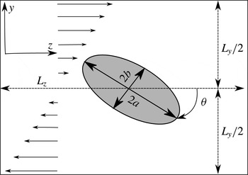
2-D schematic of the computational set-up. The simulations are in 3-D.

2.5. Computational set-up and validations
A schematic of the computational set-up is shown in figure 1. Simulations start by placing the centre of mass of the particle in the centre of the computational domain, as depicted in the figure. To accelerate the steady state, we initialized the velocity field of the domain with
 $u_{z}=\dot{{\it\gamma}}y$
, which results in a shear field as follows:
 $$\begin{eqnarray}\frac{\unicode[STIX]{x1D640}^{\infty }}{\dot{{\it\gamma}}}=\frac{1}{2}\left[\begin{array}{@{}ccc@{}}0 & 0 & 0\\ 0 & 0 & 1\\ 0 & 1 & 0\end{array}\right],\quad \frac{{\it\bf\Omega}^{\infty }}{\dot{{\it\gamma}}}=\frac{1}{2}\left[\begin{array}{@{}ccc@{}}1 & 0 & 0\end{array}\right],\end{eqnarray}$$
where
 $\unicode[STIX]{x1D640}^{\infty }$
and
 ${\it\bf\Omega}^{\infty }$
are the strain-field tensor and rotation vector of undisturbed flow. The boundary condition in the velocity gradient direction (
 $y$
-direction in figure 1) is a moving wall with velocity
 $\dot{{\it\gamma}}L_{y}/2$
in opposite directions, while the other directions are set to be periodic. The implementation of periodic boundary conditions creates a planar array of particles that rotate in phase, i.e. a periodic suspension. Such simulations can give a good approximation of a homogeneous suspension in low concentrations in which particles are sufficiently far from each other and close-distance interactions are less likely to happen. Note that, in a real suspension, particles are located randomly and rotate with a phase difference under shear, but the particle–particle interactions are low in the dilute and semi-dilute regimes. We found that the maximum fluctuations of the velocity field at the periodic boundaries are less than 5 % of the characteristic velocity
 $\dot{{\it\gamma}}a$
for the highest volume fraction
 ${\it\phi}=0.112$
and
 $\mathit{Re}=0.01$
. This shows that hydrodynamic interactions of particles at the periodic boundaries do not require a near-contact strategy and are not that significant. In addition, this boundary condition is a better approximation than the far-field boundary condition that is considered in the analytical Stokes solution for dilute regimes. The dimensions of the computational cuboid are
 $[L_{x}\times L_{y}\times L_{z}]$
, which vary from
 $[0.46a\times 2.5a\times 2.5a]$
to
 $[5a\times 5a\times 5a]$
in order to change volume fractions of suspensions for different aspect ratios.
The volume fraction of particles in suspension studies can range from very dilute to highly concentrated; for each, different assumptions and strategies are needed. At very low concentrations (dilute assumption) particles are sufficiently well separated such that any interactions between them can be assumed negligible. At slightly higher volume fractions (semi-dilute regime) particles are close enough such that they can interact hydrodynamically, but still far enough away to squeeze the flow in the small gaps between approaching particles – which can cause local viscous heating and lubrication or the formation of chains and networks of touching particles (Mueller et al.
Reference Mueller, Llewellin and Mader2010). When the concentration increases, close-distance particle interactions and particle collisions need to be taken into account, which requires collision detection and modelling of the lubrication forces (Nguyen & Ladd Reference Nguyen and Ladd2002). To avoid such difficulties, this study is aimed at dilute and semi-dilute suspensions, where particle–particle contact is not likely to happen. In addition, the Stokes number which governs the collision dynamics (Davis, Serayssol & Hinch Reference Davis, Serayssol and Hinch1986) in our simulations is always less than or equal to 10, making viscous forces dominant and the particle inertia too weak to influence the collision (Joseph et al.
Reference Joseph, Zenit, Hunt and Rosenwinkel2001). Our simulations are performed for
 $0.008\leqslant {\it\phi}\leqslant 0.112$
, for prolate ellipsoids with varying aspect ratio
 $2\leqslant \mathit{Ar}\leqslant 5$
. Following Doi & Edwards (Reference Doi and Edwards1978), for a given
 $N$
particles of length
 $L$
and diameter
 $D$
in unit volume, the dilute and semi-dilute regimes are defined as
 $N\ll 1/L^{3}$
and
 $1/L^{3}<N<1/L^{2}D$
, respectively. For an ellipsoidal particle these limits in non-dimensional form read as
 ${\it\phi}\ll ({\rm\pi}/6)\mathit{Ar}^{-2}$
and
 $({\rm\pi}/6)\mathit{Ar}^{-2}<{\it\phi}({\rm\pi}/6)<\mathit{Ar}^{-1}$
for the dilute and semi-dilute regimes, respectively. For instance, a suspension consisting of ellipsoids with aspect ratio
 $\mathit{Ar}=3$
is considered dilute if
 ${\it\phi}\ll 0.058$
, and semi-dilute if
 $0.058<{\it\phi}<0.175$
. All of the performed simulations in our study fall into the dilute and semi-dilute regimes.
The effect of Brownian motion is ignored in this work because we are focusing on the effect of inertia on the suspension under similar conditions. Furthermore, Brownian motion mainly affects the orientation distribution function of a suspension, which is irrelevant in a periodic suspension. The impact of Brownian motion is governed by the Péclet number
 $\mathit{Pe}=6{\rm\pi}{\it\mu}a^{3}\dot{{\it\gamma}}/kT$
, where
 $k=1.38\times 10^{-23}~\text{J}~\text{K}^{-1}$
is the Boltzmann constant,
 ${\it\mu}$
the dynamic viscosity of suspending liquid, and
 $T$
the absolute temperature. The Péclet number measures the strength of shearing to Brownian motion, and experiments show that the rheology of a suspension becomes independent of this parameter for
 $\mathit{Pe}>10^{3}$
(Stickel & Powell Reference Stickel and Powell2005). However, even at high
 $\mathit{Pe}$
in the limiting case of very high aspect ratios (slender particles), the dependence of the orientation of a particle on its initial orientation is much reduced (Hinch & Leal Reference Hinch and Leal1972, Reference Hinch and Leal1976; Petrie Reference Petrie1999). In this study the Peclet number is very high (
 $\mathit{Pe}\approx O(10^{5})$
, even at
 $\mathit{Re}=0.01$
and a particle dimension of a few microns) and the particle aspect ratio is
 $\mathit{Ar}\leqslant 5$
. Therefore, the effect of Brownian motion can be neglected.
In the absence of Brownian motion and particle interactions, particles with an axis of symmetry move in orbits (as will be explained in detail in § 3) which are independent of time and determined just by the initial orientations. Therefore, the initial orientation of the ellipsoids plays a very important role in the particle’s motion and stress, and consequently on the relative viscosity of the suspension. For instance, if the axis of symmetry is aligned with the vorticity vector, the particle rolls along in the flow with a steady motion (Mueller et al.
Reference Mueller, Llewellin and Mader2010), i.e. similar to a sphere. Therefore, the angular velocity and particle stress remain constant during the shear motion. In contrast, if the axis of revolution of the ellipsoid is perpendicular to the vorticity vector (
 $x$
-axis), the aspect ratio of the ellipsoid has the maximum effect on the motion and particle stress. We used this orientation for our ellipsoids to observe the maximum variation in the rheological properties of the suspension. For any other initial orientation, the effect is intermediate between the spherical and presented ellipsoidal particles, depending on the angle between the axis of revolution of the ellipsoid and the vorticity vector.
We carried out extensive validation and grid sensitivity studies to verify the reliability of our solutions – see appendix A for validation of calculations using spherical particles. For ellipsoidal particles, we used a fine surface mesh with approximately 5000–15 000 triangular elements, depending on surface area, to satisfy the required accuracy for boundary condition reconstruction as mentioned in appendix A. We also tested the grid sensitivity of the numerical results by changing the grid size from
 ${\it\Delta}=0.04a$
to
 ${\it\Delta}=0.01a$
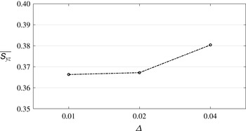
and compared the shear stresslet of particles. Figure 2 shows the results on the three grids at
 $\mathit{Re}=1.0$
and
 ${\it\phi}=0.118$
. We found the angular velocities computed on the three grids are almost identical, and the shear stresslet becomes insensitive to the grid size for
 ${\it\Delta}=0.02a$
and finer. In fact, the average values of the stresslet for the fine grid
 ${\it\Delta}=0.01a$
and the medium grid
 ${\it\Delta}=0.02a$
are very close, while for the coarse grid it is approximately 4 % higher than for the other grids. This indicates that the results are not sensitive to the grid size on the medium grid with resolution
 ${\it\Delta}=0.02a$
which is used for all the simulations reported in this work.
Grid sensitivity: the shear stresslet for a prolate ellipsoid of aspect ratio
 $\mathit{Ar}=2$
in a suspension with volume fraction
 ${\it\phi}=0.112$
at
 $\mathit{Re}=1.0$
plotted during one cycle for different grid sizes.

3. Motion of a prolate ellipsoid in a shear field
Before discussing the bulk rheology, we examine the motion of ellipsoidal particles to get a better understanding of the time (angle) dependence of the rheological parameters. In this study, we only consider prolate ellipsoids. Such particles may be characterized by the particle aspect ratio,
 $\mathit{Ar}=a/b$
, where
 $2a$
is the largest diameter of the particle on the axis of rotational symmetry (axis of revolution), and
 $2b$
is the diameter perpendicular to that axis (figure 1). We keep the largest diameter of the ellipsoid constant and change the aspect ratio to produce different ellipsoidal particles. This length is also used as the characteristic length to calculate the particle Reynolds number. As we expect, particles suspended in a viscous fluid subjected to a shear field rotate about the flow’s vorticity vector. The particle is initially aligned such that its axis of revolution (the length is shown with
 $2a$
in figure 1) is perpendicular to the vorticity vector (axis
 $x$
in our set-up). The orientation of the particle is given by
 ${\it\theta}$
, which is equal to zero when the axis of revolution is parallel to the bulk velocity (axis
 $z$
in figure 1). However, for other initial orientations, rotation of the particle’s symmetric axis defines an elliptical cone about the vorticity vector (Mueller et al.
Reference Mueller, Llewellin and Mader2010). Jeffery (Reference Jeffery1922) solved the flow around an ellipsoid under the assumption of a dilute suspension (
 ${\it\phi}\ll 1$
) and no inertial effects (
 $\mathit{Re}\rightarrow 0$
), and found the kinematics of motion for an ellipsoid to be periodic trajectories known as the ‘Jeffery orbits’. For our simulations with the aforementioned initial orientation, rotations about other axes are computed, and found to be negligible in comparison with
 $\dot{{\it\theta}}$
.
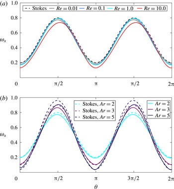
Figure 3 shows the numerical results for the angular velocity (
 ${\it\omega}_{x}=\dot{{\it\theta}}$
) for prolate (
 $\mathit{Ar}>1$
) ellipsoids as a function of the particle orientation (
 ${\it\theta}$
) during one complete cycle in comparison with the analytical solution of Jeffery (Reference Jeffery1922). As is evident in figure 3(a), our results for the ellipsoid with
 $\mathit{Ar}=2$
are very close to Jeffery’s Stokesian solution for Reynolds numbers up to
 $\mathit{Re}=1.0$
, while for higher
 $\mathit{Re}$
we observe some deviation due to the inertial effects. In fact, it can be seen in figure 3(a) that when the Reynolds number increases, the angular velocity of the particles decreases. For spheres, the angular velocity decreases and remains steady, while for ellipsoids, inertia reduces the angular velocity uniformly and does not affect the phase of motion. This is in agreement with previous studies showing that increasing the inertia would result in a reduction of the angular velocity of particles – for example, the influence of inertia on the motion of a cylindrical particle in shear flow has been predicted analytically and shown experimentally by Robertson & Acrivos (Reference Robertson and Acrivos1970). Lin et al. (Reference Lin, Peery and Schowalter1970) and Subramanian et al. (Reference Subramanian, Koch, Zhang and Yang2011) obtained an expression for the angular velocity of spheres as a function of the Reynolds number. Mikulencak & Morris (Reference Mikulencak and Morris2004) and Aidun, Lu & Ding (Reference Aidun, Lu and Ding1998) reported numerical results for the angular velocity for the case of spheres and ellipsoids, respectively, all showing a reduction of the angular velocity with increasing
 $\mathit{Re}$
. The angular acceleration, which will be discussed in § 4.2, can be obtained by differentiating the angular velocity with respect to time. We observed that the angular acceleration does not change considerably with inertia. In fact, the cycle-average amplitude of angular acceleration for
 $\mathit{Re}=0.1$
and
 $\mathit{Re}=1.0$
is approximately 6 % higher, and for
 $\mathit{Re}=10.0$
is 6 % lower than for the
 $\mathit{Re}=0.01$
regime for the suspensions shown in figure 3(a).
Instantaneous angular velocity about the vorticity vector in a shear field for a prolate ellipsoid in a suspension with volume fraction
 ${\it\phi}=0.058$
compared with Stokes solution of Jeffery for (a) a prolate ellipsoid with aspect ratio
 $\mathit{Ar}=2$
at different Reynolds numbers and (b) various aspect ratios and
 $\mathit{Re}=0.01$
.

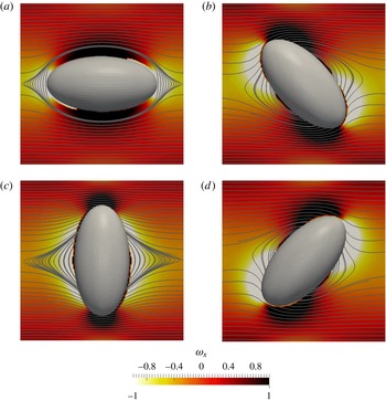
Visualization of relative vorticity (vorticity relative to undisturbed flow) and streamlines around the ellipsoid in a suspension with
 ${\it\phi}=0.058$
,
 $\mathit{Ar}=2$
,
 $\mathit{Re}=0.01$
. (a) Minimum angular velocity,
 ${\it\theta}=0$
; (b) maximum acceleration,
 ${\it\theta}={\rm\pi}/4$
; (c) maximum angular velocity,
 ${\it\theta}={\rm\pi}/2$
; (d) maximum deceleration,
 ${\it\theta}=3{\rm\pi}/4$
.

In figure 3(b), the angular velocities of ellipsoids with different aspect ratios are compared with their corresponding analytical Stokes solution. The angular velocity is maximum at
 ${\it\theta}={\rm\pi}/2$
and
 ${\it\theta}=3{\rm\pi}/2$
, and minimum at
 ${\it\theta}=0$
and
 ${\it\theta}={\rm\pi}$
, for which the projected area against the flow is maximum and minimum, respectively. It can be observed that the amplitude of
 ${\it\omega}_{x}$
increases as the aspect ratio is increased (figure 3
b). For a sphere in Stokes flow, this amplitude is equal to 0.5, while for high aspect ratio ellipsoids it approaches 1 (Jeffery Reference Jeffery1922). The trend in figure 3(b) is consistent with the Jeffery (Reference Jeffery1922) analytical solution for the
 $\mathit{Re}=0$
limit, and the reduction in angular velocity around
 ${\it\theta}={\rm\pi}/2,3{\rm\pi}/2$
is due to inertial effects.
In figure 4 the out-of-plane vorticity contours and streamlines around the ellipsoid are visualized in the symmetric midplane (plane perpendicular to the vorticity vector and passing the centre of the ellipsoid) for different phases in a suspension with
 $\mathit{Re}=0.01$
and
 ${\it\phi}=0.058$
. The background plane is coloured by the relative out-of-plane vorticity (vorticity relative to the undisturbed flow), where dark and bright colours indicate positive and negative vorticity regions, respectively. Figure 4(a) shows the ellipsoid at
 ${\it\theta}=0$
, where the angular velocity is minimum (figure 3
a), and we can clearly see the closed streamline region around the ellipsoid. The existence of this region was shown numerically by Kossack & Acrivos (Reference Kossack and Acrivos1974) and experimentally verified by Poe & Acrivos (Reference Poe and Acrivos1975) for spheres and cylinders. The other instances visualized in figure 4 show that the closing streamline region would collapse by rotation of the ellipsoid. As we can see in figure 4(b–d), when the ellipsoid is not aligned with the flow, the curvature of the body twists the streamlines and disturbs the closing region around the particle. In figure 4(a), we see that a negative vorticity region is formed at both poles of the particle, i.e. the flow in these regions rotates in a direction opposite to the undisturbed shear flow. In contrast, when the particle reaches the maximum angular velocity (see figure 4
c), negative vorticity regions are formed near the sides of the particle. At
 ${\it\theta}={\rm\pi}/4$
and
 ${\it\theta}=3{\rm\pi}/4$
, (Figure 4
b,d, respectively), we can observe that the curvature of flow changes at the poles, i.e. the direction of vorticity changes at the poles.
4. Instantaneous bulk particle stress
In this part, we provide the numerically computed bulk (volume-averaged) rheological properties of suspensions for the smallest time scale (as a function of particle orientation) at varying volume fraction (
 ${\it\phi}$
), Reynolds number (
 $\mathit{Re}$
) and particle shape (
 $\mathit{Ar}$
). The viscometric functions of a suspension
 $({\it\eta}_{r},N_{1},N_{2})$
, are functions of the volume-averaged particle stress tensor (2.15). Therefore, these rheological parameters consist of three components of the particle stress, i.e. the stresslet, the acceleration stress, and the Reynolds stress (2.13). We discuss the effect of an ellipsoid’s aspect ratio and volume fraction at various ranges of Reynolds number on each component of these parameters separately. For ellipsoidal particles, the particle stress is a function of the orientation and we expect a quasisteady state when
 $t\rightarrow \infty$
. Therefore, we let the simulations continue until the quasisteady state condition is reached for all the plots of this section. The cycle-average value and cycle-average standard deviation (denoted by
 ${\it\sigma}$
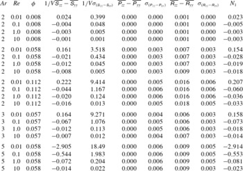
) of these plots can be found in tables 1–3.
4.1. Stresslet
The dominant part of a hydrodynamic stress system in the suspension due to the presence of particles is the symmetric part of the first moment of stress calculated on the surface of particles, called the stresslet. Based on (2.13) and (2.15), the contribution of the stresslet to the normal stress differences and the relative viscosity,
 $N_{1}$
,
 $N_{2}$
and
 ${\it\eta}_{r}$
are proportional to
 $\unicode[STIX]{x1D61A}_{zz}-\unicode[STIX]{x1D61A}_{yy}$
,
 $\unicode[STIX]{x1D61A}_{yy}-\unicode[STIX]{x1D61A}_{xx}$
and
 $\unicode[STIX]{x1D61A}_{yz}$
, respectively. To identify the role of inertia and verify our results, we compare our results against the analytical solution of a single ellipsoid at
 $(\mathit{Re},{\it\phi})\rightarrow 0$
(Kim & Karrila Reference Kim and Karrila2013) – see appendix B.
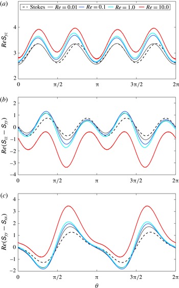
In figure 5, the Reynolds-scaled stresslet for a ellipsoid with aspect ratio
 $\mathit{Ar}=2$
in a suspension of volume fraction
 ${\it\phi}=0.058$
at various Reynolds numbers is compared with the analytical solution during one complete rotation about its centre of mass. The numerical stresslet calculation is verified by comparing it to the analytical calculation in figure 5, as it follows the same trend, has similar phases and amplitudes as the analytical values, and the deviations are the results of inertia, which increase as Re increases. The influence of inertia on the stresslet can easily be seen in figure 5. It can be observed that, as inertia increases, the shear stresslet
 $\mathit{Re}\unicode[STIX]{x1D61A}_{yz}$
and the second normal stresslet difference
 $\mathit{Re}(\unicode[STIX]{x1D61A}_{yy}-\unicode[STIX]{x1D61A}_{xx})$
increase, whereas the first normal stresslet difference
 $\mathit{Re}(\unicode[STIX]{x1D61A}_{zz}-\unicode[STIX]{x1D61A}_{yy})$
decreases during the cycle. However, the inertial effects on the these components of the stresslets are not uniform. For instance, deviation from the analytical solution in the shear stresslet is higher in some phases, or in the normal stresslet differences, inertia increases or decreases the stresslet depending on the orientation of particles. This asymmetrical growth is due to the fact that inertia acts differently on each component of the stresslet: the strain-field stresslet
 $\unicode[STIX]{x1D64E}^{\unicode[STIX]{x1D640}}$
, and the rotational stresslet
 $\unicode[STIX]{x1D64E}^{{\it\bf\Omega}}$
.
Instantaneous shear stresslet (a) and normal stresslet differences (b) and (c), as a function of orientation for a prolate ellipsoid of aspect ratio
 $\mathit{Ar}=2$
in a suspension with volume fraction
 ${\it\phi}=0.058$
at various Reynolds numbers are compared with the exact solution of Kim & Karrila (Reference Kim and Karrila2013).

The particle’s stresslet is generated by two mechanisms based on the analytical solution of a single prolate ellipsoid in the linear flow field, i.e. the superposition of a rotation
 ${\it\bf\Omega}^{\infty }$
and a strain field
 $\unicode[STIX]{x1D640}^{\infty }$
(Kim & Karrila Reference Kim and Karrila2013) – see appendix B and (B 1):
 $$\begin{eqnarray}\displaystyle & \displaystyle \mathit{Re}\unicode[STIX]{x1D61A}_{yz}=\mathit{Re}\unicode[STIX]{x1D61A}_{yz}^{\unicode[STIX]{x1D640}}+\mathit{Re}\unicode[STIX]{x1D61A}_{yz}^{{\it\bf\Omega}}, & \displaystyle\end{eqnarray}$$
 $$\begin{eqnarray}\displaystyle & \displaystyle \mathit{Re}(\unicode[STIX]{x1D61A}_{zz}-\unicode[STIX]{x1D61A}_{yy})=\mathit{Re}(\unicode[STIX]{x1D61A}_{zz}^{\unicode[STIX]{x1D640}}-\unicode[STIX]{x1D61A}_{yy}^{\unicode[STIX]{x1D640}})+\mathit{Re}(\unicode[STIX]{x1D61A}_{zz}^{{\it\bf\Omega}}-\unicode[STIX]{x1D61A}_{yy}^{{\it\bf\Omega}}), & \displaystyle\end{eqnarray}$$
 $$\begin{eqnarray}\displaystyle & \displaystyle \mathit{Re}(\unicode[STIX]{x1D61A}_{yy}-\unicode[STIX]{x1D61A}_{xx})=\mathit{Re}(\unicode[STIX]{x1D61A}_{yy}^{\unicode[STIX]{x1D640}}-\unicode[STIX]{x1D61A}_{xx}^{\unicode[STIX]{x1D640}})+\mathit{Re}(\unicode[STIX]{x1D61A}_{yy}^{{\it\bf\Omega}}-\unicode[STIX]{x1D61A}_{xx}^{{\it\bf\Omega}}), & \displaystyle\end{eqnarray}$$
 $\unicode[STIX]{x1D640}$
and
 ${\it\bf\Omega}$
denote the strain and the rotational parts of the stresslet, respectively. The right-hand side of (4.1c
) for a prolate ellipsoid rotating in the
 $C=\infty$
orbit (shown in figure 4) is given by (Kim & Karrila Reference Kim and Karrila2013):
 $$\begin{eqnarray}\displaystyle & \displaystyle \mathit{Re}\unicode[STIX]{x1D61A}_{yz}^{\unicode[STIX]{x1D640}}=\frac{20{\rm\pi}}{3}[F_{1}(\mathit{Ar})\sin ^{2}(2{\it\theta})+F_{2}(\mathit{Ar})]\unicode[STIX]{x1D60C}_{yz}, & \displaystyle\end{eqnarray}$$
 $$\begin{eqnarray}\displaystyle & \displaystyle \mathit{Re}(\unicode[STIX]{x1D61A}_{zz}^{\unicode[STIX]{x1D640}}-\unicode[STIX]{x1D61A}_{yy}^{\unicode[STIX]{x1D640}})=\frac{20{\rm\pi}}{3}F_{3}(\mathit{Ar})\sin (4{\it\theta})\unicode[STIX]{x1D60C}_{yz}, & \displaystyle\end{eqnarray}$$
 $$\begin{eqnarray}\displaystyle & \displaystyle \mathit{Re}(\unicode[STIX]{x1D61A}_{yy}^{\unicode[STIX]{x1D640}}-\unicode[STIX]{x1D61A}_{xx}^{\unicode[STIX]{x1D640}})=\frac{20{\rm\pi}}{3}\sin (2{\it\theta})[F_{4}(\mathit{Ar})\cos (2{\it\theta})+F_{5}(\mathit{Ar})]\unicode[STIX]{x1D60C}_{yz}, & \displaystyle\end{eqnarray}$$
 $$\begin{eqnarray}\displaystyle & \displaystyle \mathit{Re}\unicode[STIX]{x1D61A}_{yz}^{{\it\bf\Omega}}=4{\rm\pi}F_{6}(\mathit{Ar})\cos (2{\it\theta})({\it\Omega}_{x}^{\infty }-{\it\omega}_{x}), & \displaystyle\end{eqnarray}$$
 $$\begin{eqnarray}\displaystyle & \displaystyle \mathit{Re}(\unicode[STIX]{x1D61A}_{zz}^{{\it\bf\Omega}}-\unicode[STIX]{x1D61A}_{yy}^{{\it\bf\Omega}})=4{\rm\pi}F_{7}(\mathit{Ar})\sin (2{\it\theta})({\it\Omega}_{x}^{\infty }-{\it\omega}_{x}), & \displaystyle\end{eqnarray}$$
 $$\begin{eqnarray}\displaystyle & \displaystyle \mathit{Re}(\unicode[STIX]{x1D61A}_{yy}^{{\it\bf\Omega}}-\unicode[STIX]{x1D61A}_{xx}^{{\it\bf\Omega}})=4{\rm\pi}F_{8}(\mathit{Ar})\sin (2{\it\theta})({\it\Omega}_{x}^{\infty }-{\it\omega}_{x}), & \displaystyle\end{eqnarray}$$
 $F_{i}$
are functions of the aspect ratio
 $\mathit{Ar}$
, and
 ${\it\theta}$
is measured as shown in figure 1. We will focus on the influence of inertia on the rotation and strain-field stresslet mechanisms to explain the variation of shear and normal stresslets with Reynolds number.
4.1.1. Shear stresslet
The instantaneous shear stresslet shown in figure 5(a) consists of the strain-field shear stresslet
 $\mathit{Re}\unicode[STIX]{x1D61A}_{yz}^{\unicode[STIX]{x1D640}}$
and the rotational shear stresslet
 $\mathit{Re}\unicode[STIX]{x1D61A}_{yz}^{{\it\bf\Omega}}$
. The strain-field shear stresslet does not vary considerably over the cycle – for instance, the maximum amplitude of its variation is less than 2 % of its average value for
 $\mathit{Ar}=2$
. Maximum values of
 $\mathit{Re}\unicode[STIX]{x1D61A}_{yz}^{\unicode[STIX]{x1D640}}$
occur at
 ${\it\theta}=0,{\rm\pi}/2,{\rm\pi},3{\rm\pi}/2$
, when the resistance to the strain is maximum. Minimum values of
 $\mathit{Re}\unicode[STIX]{x1D61A}_{yz}^{\unicode[STIX]{x1D640}}$
occur at
 ${\it\theta}={\rm\pi}/4,3{\rm\pi}/4,5{\rm\pi}/4,7{\rm\pi}/4$
, when the longest diameter of the particle is aligned with the strain axis and, consequently, the resistant force against the strain is minimum. For a spherical particle, this term is the only source of stresslet generation and its value remains constant. On the other hand, for the rotational part of the shear stresslet,
 $\mathit{Re}\unicode[STIX]{x1D61A}_{yz}^{{\it\bf\Omega}}$
is proportional to the angular velocity difference between the flow and the particle, as is evident from (4.2). For ellipsoids, when
 $\mathit{Ar}\rightarrow 1$
(i.e. to sphere) and the angular velocity of the particle
 ${\it\omega}_{x}\rightarrow 0.5$
, consequently,
 $\mathit{Re}\unicode[STIX]{x1D61A}_{yz}^{{\it\bf\Omega}}$
goes to zero. For ellipsoids,
 $\mathit{Re}\unicode[STIX]{x1D61A}_{yz}^{{\it\bf\Omega}}$
is always negative, except when the angular velocity of the body is equal to the rotation of the flow (
 ${\it\theta}={\rm\pi}/4,3{\rm\pi}/4,5{\rm\pi}/4,7{\rm\pi}/4$
in figure 3), which makes the rotational stresslet zero (maximum value in the cycle). When the angular velocities of the particle and rotation vector of the flow have their maximum difference (
 ${\it\theta}=0,{\rm\pi}/2,{\rm\pi},3{\rm\pi}/2$
in figure 3),
 $\mathit{Re}\unicode[STIX]{x1D61A}_{yz}^{{\it\bf\Omega}}$
is minimum, and adding this negative value to the strain-field stresslet results in minimum values of the total stresslet shown in figure 5(a).
For
 $\mathit{Re}=0.01$
, only a small deviation from the Stokesian solution is observed around
 ${\it\theta}=0,{\rm\pi}/2,{\rm\pi},3{\rm\pi}/2$
in figure 5(a). Considering figure 3(a), these points correspond to a small deviation from the analytical solution for the angular velocity. By increasing the inertia to the order of
 $\mathit{Re}=O(1)$
, the amplitude of the stresslet grows in all phases even though the angular velocity of the particle has not changed with respect to the highly viscous regime of
 $\mathit{Re}=0.01$
(figure 3
a). Comparing instantaneous stresslet curves for
 $\mathit{Re}=0.1$
and
 $\mathit{Re}=1.0$
with that at
 $\mathit{Re}=0.01$
, it can be seen that inertial forces effectively increase the value of the shear strain-field stresslet. This effect can be observed more clearly at
 ${\it\theta}={\rm\pi}/4,3{\rm\pi}/4,5{\rm\pi}/4,7{\rm\pi}/4$
, where the rotational stresslet,
 $\mathit{Re}\unicode[STIX]{x1D61A}_{yz}^{{\it\bf\Omega}}$
, is zero (because of a zero angular velocity difference between the particle and the flow). The influence of inertia on the increase in the shear strain-field stresslet in ellipsoids agrees well with the results for spheres (spherical particles experience stresslets only because of the strain field), which show an increase in the stresslet with an increase in
 $\mathit{Re}$
(Lin et al.
Reference Lin, Peery and Schowalter1970; Mikulencak & Morris Reference Mikulencak and Morris2004; Subramanian et al.
Reference Subramanian, Koch, Zhang and Yang2011; Haddadi & Morris Reference Haddadi and Morris2014). At
 ${\it\theta}=0,{\rm\pi}$
the angular velocity difference (
 ${\it\Omega}_{x}^{\infty }-{\it\omega}_{x}$
) is higher relative to the Stokes regimes. Consequently, the effect of the rotational stresslet is higher, and can eliminate the increase in the strain-field stresslet. That is why we see minimal differences between the Stokesian and computational results at these phases.
For the moderate inertial regime of
 $\mathit{Re}=10$
, figure 5(a) reveals that the increase of the strain-field shear stresslet (
 $\mathit{Re}\unicode[STIX]{x1D61A}_{yz}^{\unicode[STIX]{x1D640}}$
) due to the inertial effect has intensified. This effect can be clearly seen by considering phases corresponding to a zero rotational stresslet (
 ${\it\theta}={\rm\pi}/4,3{\rm\pi}/4,5{\rm\pi}/4,7{\rm\pi}/4$
, where the angular velocity difference is zero). The peak values of the rotational shear stresslet (
 $\mathit{Re}\unicode[STIX]{x1D61A}_{yz}^{{\it\bf\Omega}}$
) become greater due to the higher angular velocity difference at
 ${\it\theta}=0,{\rm\pi}$
. However, this term cannot eliminate the effect of inertia on the strain-field stresslet similar to the previously discussed low inertial regimes. Therefore, at these phases the net total shear stresslet is higher than the Stokes solution. At
 ${\it\theta}={\rm\pi}/2,3{\rm\pi}/2$
the rotational stresslet becomes weaker since the maximum velocity of the particles decreases relative to the analytical solution, resulting in a smaller value of (
 ${\it\Omega}_{x}^{\infty }-{\it\omega}_{x}$
). Consequently, at these phases, we witness a greater deviation from the Stokes solution than for
 ${\it\theta}=0,{\rm\pi}$
.
Considering all the
 $\mathit{Re}$
values discussed in figure 5(a), we can conclude that inertia would increase the stresslet of suspensions consisting of ellipsoidal particles due to the strain-field stresslet mechanism,
 $\unicode[STIX]{x1D64E}^{\unicode[STIX]{x1D640}}$
. The other mechanism of stresslet generation,
 $\unicode[STIX]{x1D64E}^{{\it\bf\Omega}}$
, acts in the opposite way and acts to cancel the strain-field stresslet, i.e. the absolute value of the rotational stresslet increases with inertia, but its negative value opposes the strain-field stresslet.
4.1.2. Normal stresslet differences
Based on (4.1b
) and (4.1c
), the normal stresslet differences shown in figure 5(b,c) are composed of the strain-field stresslet and the rotational stresslet, similar to the shear stresslet. The analytical solution for all components of the normal stresslet differences,
 $\mathit{Re}(\unicode[STIX]{x1D61A}_{zz}^{\unicode[STIX]{x1D640}}-\unicode[STIX]{x1D61A}_{yy}^{\unicode[STIX]{x1D640}})$
,
 $\mathit{Re}(\unicode[STIX]{x1D61A}_{yy}^{\unicode[STIX]{x1D640}}-\unicode[STIX]{x1D61A}_{xx}^{\unicode[STIX]{x1D640}})$
,
 $\mathit{Re}(\unicode[STIX]{x1D61A}_{zz}^{{\it\bf\Omega}}-\unicode[STIX]{x1D61A}_{yy}^{{\it\bf\Omega}})$
, and
 $\mathit{Re}(\unicode[STIX]{x1D61A}_{yy}^{{\it\bf\Omega}}-\unicode[STIX]{x1D61A}_{xx}^{{\it\bf\Omega}})$
are sinusoidal symmetric functions that oscillate about zero. Therefore, the superposition of these analytical functions is symmetric about zero as well.
Plots of the normal stresslet differences in figure 5(b,c) show a clear distinction between the suspension at
 $\mathit{Re}=10$
and lower inertial regimes. For simulations up to
 $\mathit{Re}=1.0$
, inertia decreases
 $\mathit{Re}(\unicode[STIX]{x1D61A}_{zz}-\unicode[STIX]{x1D61A}_{yy})$
and increases
 $\mathit{Re}(\unicode[STIX]{x1D61A}_{yy}-\unicode[STIX]{x1D61A}_{xx})$
, except for two intervals
 $0<{\it\theta}<{\rm\pi}/2$
and
 ${\rm\pi}<{\it\theta}<3{\rm\pi}/2$
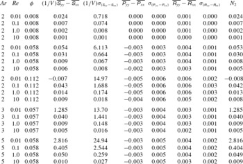
(note the negative average value of the first normal stresslet difference and the positive value of the second normal stresslet difference in tables 2 and 3, respectively). Asymptotic solutions of Lin et al. (Reference Lin, Peery and Schowalter1970) and Subramanian et al. (Reference Subramanian, Koch, Zhang and Yang2011) for suspensions consisting of spherical particles show that inertia makes the normal stresslet differences,
 $\unicode[STIX]{x1D61A}_{zz}-\unicode[STIX]{x1D61A}_{yy}$
and
 $\unicode[STIX]{x1D61A}_{yy}-\unicode[STIX]{x1D61A}_{xx}$
negative and positive, respectively. As mentioned earlier for the shear stresslet, and considering (4.2), the rotational part of the stresslet is zero for spherical particles. Therefore, we can conclude that
 $\mathit{Re}(\unicode[STIX]{x1D61A}_{zz}^{\unicode[STIX]{x1D640}}-\unicode[STIX]{x1D61A}_{yy}^{\unicode[STIX]{x1D640}})$
should increase and
 $\mathit{Re}(\unicode[STIX]{x1D61A}_{yy}^{\unicode[STIX]{x1D640}}-\unicode[STIX]{x1D61A}_{xx}^{\unicode[STIX]{x1D640}})$
should decrease at all phases with inertia (assuming the same trend for ellipsoids and spheres for the effect of inertia on the strain-field components of the normal stresslet differences). Simultaneously, the rotational components of the normal stresslet differences,
 $\mathit{Re}(\unicode[STIX]{x1D61A}_{yy}^{{\it\bf\Omega}}-\unicode[STIX]{x1D61A}_{xx}^{{\it\bf\Omega}})$
and
 $\mathit{Re}(\unicode[STIX]{x1D61A}_{zz}^{{\it\bf\Omega}}-\unicode[STIX]{x1D61A}_{yy}^{{\it\bf\Omega}})$
, seem to increase the amplitude of oscillations (figure 5
b,c). The asymmetric change of peaks is due to a small non-uniform reduction in the angular velocity of the particles, which makes the rotational component of the normal stresslet asymmetric.
For
 $\mathit{Re}=10$
, the first normal stresslet difference is lower than the Stokesian solution, whereas the second normal stresslet difference is higher than the corresponding Stokesian solution for all phases (figure 5
b,c). This is due to the fact that the strain-field components,
 $\mathit{Re}(\unicode[STIX]{x1D61A}_{zz}^{\unicode[STIX]{x1D640}}-\unicode[STIX]{x1D61A}_{yy}^{\unicode[STIX]{x1D640}})$
and
 $\mathit{Re}(\unicode[STIX]{x1D61A}_{yy}^{\unicode[STIX]{x1D640}}-\unicode[STIX]{x1D61A}_{xx}^{\unicode[STIX]{x1D640}})$
, become dominant over the rotational components, considerably decreasing
 $\mathit{Re}(\unicode[STIX]{x1D61A}_{zz}-\unicode[STIX]{x1D61A}_{yy})$
and increasing
 $\mathit{Re}(\unicode[STIX]{x1D61A}_{yy}-\unicode[STIX]{x1D61A}_{xx})$
for this regime of flow.
4.2. Acceleration stress
We discussed in § 4.1 how inertia affects the total particle stress of the suspension (by increasing the shear stresslet
 $\unicode[STIX]{x1D61A}_{yz}$
and the second normal stresslet difference
 $\unicode[STIX]{x1D61A}_{yy}-\unicode[STIX]{x1D61A}_{xx}$
and decreasing the first normal stresslet difference
 $\unicode[STIX]{x1D61A}_{zz}-\unicode[STIX]{x1D61A}_{yy}$
of the suspension). However, this is not the sole effect of inertia on the rheology of suspension. Based on (2.13), inertia plays a direct role in the total particle stress by generating acceleration and Reynolds stresses, which will be discussed in more detail in this subsection and § 4.3. Acceleration stress, by definition, is generated by the acceleration of particles moving within the suspension ((2.12) and (2.14b
)). Similar to § 4.1, we have derived the analytical expression based on the Stokes solution of the problem (appendix C) to verify our numerical results, have a better understanding of the nature of this term, and establish the effect of inertia by comparing it against our solutions. It is worth noting that the particle acceleration is calculated based on the rotation of the particle, and translational acceleration has been ignored due to the fact that the centre of mass of the particle is located on the zero surface of shear, and the net of the force exerted on the particle is negligible. In appendix C, we obtain a formula for the acceleration stress of any arbitrarily shaped particle based on the Stokesian solution of Jeffery (Reference Jeffery1922) (assuming a particle rotating in the
 $C=\infty$
orbit). For our ellipsoidal particles, this formulation can be simplified and expressed in terms of the volume fraction, aspect ratio and angular kinematics of the particle as:
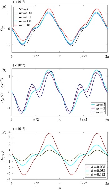
 $$\begin{eqnarray}\displaystyle & \displaystyle \unicode[STIX]{x1D617}_{yz}=\frac{1}{10}{\it\phi}\left(1-\frac{1}{\mathit{Ar}^{2}}\right)({\it\alpha}_{x}\cos (2{\it\theta})-{\it\omega}_{x}^{2}\sin (2{\it\theta})),\qquad & \displaystyle\end{eqnarray}$$
 $$\begin{eqnarray}\displaystyle & \displaystyle \unicode[STIX]{x1D617}_{zz}-\unicode[STIX]{x1D617}_{yy}=\frac{1}{5}{\it\phi}\left(1-\frac{1}{\mathit{Ar}^{2}}\right)({\it\alpha}_{x}\sin (2{\it\theta})+{\it\omega}_{x}^{2}\cos (2{\it\theta})),\qquad & \displaystyle\end{eqnarray}$$
 $$\begin{eqnarray}\displaystyle & \displaystyle \unicode[STIX]{x1D617}_{yy}-\unicode[STIX]{x1D617}_{xx}=\frac{-1}{10}{\it\phi}\left[\left(1-\frac{1}{\mathit{Ar}^{2}}\right)({\it\alpha}_{x}\sin (2{\it\theta})+{\it\omega}_{x}^{2}\cos (2{\it\theta}))+\left(1+\frac{1}{\mathit{Ar}^{2}}\right){\it\omega}_{x}^{2}\right],\qquad & \displaystyle\end{eqnarray}$$
 ${\it\alpha}_{x}$
is the angular acceleration in the vorticity direction and (
 $\unicode[STIX]{x1D617}_{yz}$
,
 $\unicode[STIX]{x1D617}_{zz}-\unicode[STIX]{x1D617}_{yy}$
,
 $\unicode[STIX]{x1D617}_{yy}-\unicode[STIX]{x1D617}_{xx}$
) will be referred to as the shear acceleration stress, first normal acceleration stress difference, and second normal acceleration stress difference, respectively. In the remainder of this subsection we discuss the effect of the volume fraction, aspect ratio and inertia on the shear and normal components of the instantaneous acceleration stress.
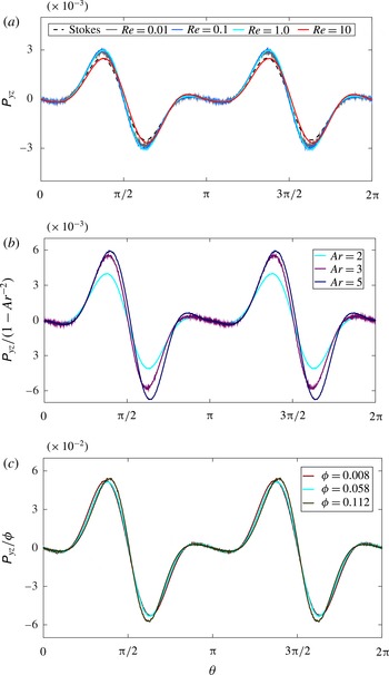
Shear acceleration stress as a function of orientation for a suspension of (a) prolate ellipsoids with aspect ratio
 $\mathit{Ar}=2$
at different Reynolds numbers and volume fraction
 ${\it\phi}=0.058$
, (b) ellipsoids with various aspect ratios at
 $\mathit{Re}=1$
and volume fraction
 ${\it\phi}=0.058$
, and (c) ellipsoids with aspect ratio
 $\mathit{Ar}=2$
and
 $\mathit{Re}=1$
at different volume fractions.

4.2.1. Shear acceleration stress
In figure 6(a), the shear acceleration stress for an ellipsoid with aspect ratio
 $\mathit{Ar}=2$
in a suspension of volume fraction
 ${\it\phi}=0.058$
is shown at various Reynolds numbers and compared with the analytical Stokes solution (4.3a
). It can be observed that the inertia does not affect the acceleration stress considerably, and our numerical results are generally close to the analytical solution. In the moderate inertial regime
 $\mathit{Re}=10$
, the amplitude of the acceleration stress decreases slightly relative to the lower inertial regimes (note the difference in the average variation of the shear acceleration stress
 ${\it\sigma}_{\unicode[STIX]{x1D617}_{yz}}$
between
 $\mathit{Re}=10$
and other values of
 $\mathit{Re}$
for the discussed volume fraction and aspect ratio in table 1).
Equation (4.3a
) illustrates the dependence of the shear acceleration stress on the aspect ratio and volume fraction based on the Stokesian solution. We observe that for spherical particles (
 $\mathit{Ar}=1$
) the acceleration stress is almost zero. This is in agreement with the analytical solution (4.3a
) and the numerical simulations of Haddadi & Morris (Reference Haddadi and Morris2014). In order to verify the possible proportionality of this term to the factors
 $1-\mathit{Ar}^{-2}$
and
 ${\it\phi}$
, as appears in (4.3a
), we plot
 $\unicode[STIX]{x1D617}_{yz}/(1-\mathit{Ar}^{-2})$
and
 $\unicode[STIX]{x1D617}_{yz}/{\it\phi}$
in figure 6(b,c), respectively. Figure 6(b) shows the shear acceleration stress for suspensions consisting of ellipsoids with three different aspect ratios at equal volume fractions and Reynolds numbers. All particles have peaks at approximately the same phase, and the amplitude of the shear acceleration stress increases with the aspect ratio. This figure clearly shows that the shear acceleration stress increases with aspect ratio more than expected according to the analytical solution, i.e. the shear acceleration stress is not proportional to
 $1-\mathit{Ar}^{-2}$
. This higher increase is probably due to the fact that the angular velocity and acceleration have a greater deviation from the analytical Stokesian solution when the aspect ratio increases (figure 3). However, comparing
 ${\it\sigma}_{\unicode[STIX]{x1D617}_{yz}}$
for different particles in table 1, this increase in the peaks has a minor influence on the average variation of the shear acceleration stress.
Figure 6(c) shows the acceleration stress per unit volume fraction for a suspension of ellipsoids with aspect ratio
 $\mathit{Ar}=2$
at
 $\mathit{Re}=1.0$
at three different volume fractions. As is evident in the figure, and in contrast to the aspect ratio, the amplitude of the shear acceleration stress increases proportionally to the volume fraction of the suspension. For very dilute suspensions
 ${\it\phi}<0.01$
, our results in figure 6(c) and table 1 show that this component has no effect on the particle stress (neither the cycle average, nor the average variation), regardless of Reynolds number.
Considering the different parts of figure 6 and the calculations of the average values in table 1, one can easily see that the shear acceleration stress is a symmetric variable about zero, i.e. its cycle average is zero for all cases. This component of the shear particle stress is not significantly influenced by inertia, whereas its amplitude can increase with the aspect ratio and volume fraction.
4.2.2. Normal acceleration stress differences
Similar to the shear acceleration stress, numerical results for the normal acceleration stress differences,
 $\unicode[STIX]{x1D617}_{zz}-\unicode[STIX]{x1D617}_{yy}$
and
 $\unicode[STIX]{x1D617}_{yy}-\unicode[STIX]{x1D617}_{xx}$
, are first compared with their corresponding Stokesian solutions at various inertial regimes in figures 7(a) and 8(a) to reveal the influence of inertia on these parameters. Analogous to the shear component, all inertial results for normal differences are in good agreement with the Stokesian solutions. In fact, inertia seems to have the least effect on the normal acceleration stress difference, and only at
 $\mathit{Re}=10$
the peaks are slightly decreased relative to lower Reynolds numbers.
First normal acceleration stress difference as a function of orientation for a suspension of (a) prolate ellipsoids with aspect ratio
 $\mathit{Ar}=2$
at different Reynolds numbers and volume fraction
 ${\it\phi}=0.058$
, (b) ellipsoids with various aspect ratios at
 $\mathit{Re}=1$
and volume fraction
 ${\it\phi}=0.058$
, and (c) ellipsoids with aspect ratio
 $\mathit{Ar}=2$
and
 $\mathit{Re}=1$
at different volume fractions.

Second normal acceleration stress difference as a function of orientation for a suspension of (a) prolate ellipsoids with aspect ratio
 $\mathit{Ar}=2$
at different Reynolds numbers and volume fraction
 ${\it\phi}=0.058$
, (b) ellipsoids with various aspect ratios at
 $\mathit{Re}=1$
and volume fraction
 ${\it\phi}=0.058$
, and (c) ellipsoids with aspect ratio
 $\mathit{Ar}=2$
and
 $\mathit{Re}=1$
at different volume fractions.

The most important point about
 $\unicode[STIX]{x1D617}_{zz}-\unicode[STIX]{x1D617}_{yy}$
and
 $\unicode[STIX]{x1D617}_{yy}-\unicode[STIX]{x1D617}_{xx}$
is that, in contrast to the shear component, the normal acceleration differences are highly asymmetric about zero in two different ways. While the first normal acceleration stress
 $\unicode[STIX]{x1D617}_{zz}-\unicode[STIX]{x1D617}_{yy}$
oscillates between negative and positive values, with a zero cycle-average value for all cases (table 2), the second normal acceleration stress
 $\unicode[STIX]{x1D617}_{yy}-\unicode[STIX]{x1D617}_{xx}$
is almost negative, with comparable average variation about the cycle averages (notice the standard deviation of these components in tables 2 and 3). Comparing (4.3a
), (4.3b
) and (4.3c
), we see that, in contrast to
 $\unicode[STIX]{x1D617}_{yz}$
and
 $\unicode[STIX]{x1D617}_{zz}-\unicode[STIX]{x1D617}_{yy}$
, a considerable negative term (last term in the bracket) exists in
 $\unicode[STIX]{x1D617}_{yy}-\unicode[STIX]{x1D617}_{xx}$
, making the second acceleration stress always negative. This is important because the non-zero cycle-average value of the acceleration stress plays an important role in the cycle-average value of the second normal stress difference, as will be discussed in § 5.
The effects of the aspect ratio and volume fraction of this component of the normal stress differences are almost identical to the shear acceleration stress. Figures 7(b) and 8(b) show the normal acceleration stress differences, scaled with
 $1-\mathit{Ar}^{-2}$
(to be consistent with the shear acceleration stress in figure 6
b), for three different ellipsoids at equal particle concentration and inertia. All particles have peaks at approximately the same phase, and the peaks of the oscillations increase with the aspect ratio (for ellipsoids with
 $\mathit{Ar}=5$
, the growth of the peaks around
 ${\it\theta}=0,{\rm\pi}$
is asymmetric). One can easily observe that, similar to the shear acceleration stress, the normal acceleration stress increases faster than
 $1-\mathit{Ar}^{-2}$
, even though this increase has no effect on the cycle averages of the normal acceleration stress, and only increases the average variations,
 ${\it\sigma}_{(\unicode[STIX]{x1D617}_{zz}-\unicode[STIX]{x1D617}_{yy})}$
and
 ${\it\sigma}_{(\unicode[STIX]{x1D617}_{yy}-\unicode[STIX]{x1D617}_{xx})}$
– see tables 2 and 3.
The other influential parameter on the normal acceleration stress is the particle concentration. Figures 7(c) and 8(c) show the normal acceleration stress differences for a suspension of ellipsoids with aspect ratio
 $\mathit{Ar}=2$
at
 $\mathit{Re}=1.0$
at three different volume fractions. Both figures, and the corresponding cycle averages and average variations in tables 2 and 3, indicate that the normal acceleration stress increases proportionally with the volume fraction of the suspension. This component of the particle stress becomes important for
 ${\it\phi}\sim O(0.05)$
or higher, and for very dilute suspensions its cycle average and average variation are negligible.
4.3. Reynolds stress
The last term on the right-hand side of (2.11) is the stress generated due to disturbances caused by the motion of particles in the flow. Mathematically, the Reynolds stress originates from the nonlinear (inertial) term of the Navier–Stokes equations. Physically speaking, interactions between the particles themselves and the flow cause velocity fluctuations for both the particles and the flow. Reynolds stress, as defined in (2.14c
), is the volume average of the velocity fluctuation products for the entire suspension volume (
 $V=V_{f}+V_{p}$
). Yeo & Maxey (Reference Yeo and Maxey2013) considered just the fluid part in the formulation of particle stress and ignored this term for the range
 $\mathit{Re}\leqslant 2.0$
. Kulkarni & Morris (Reference Kulkarni and Morris2008) considered both parts for the Reynolds stress and reported a linear increase of this term with respect to
 $\mathit{Re}$
. Both studies concluded that, for spherical particles, the Reynolds stress is negligible for flow regimes in the range
 $\mathit{Re}\sim O(1)$
. Recently, Haddadi & Morris (Reference Haddadi and Morris2014) investigated a dense suspension of spheres and found that the Reynolds stress influences the total second normal stress considerably when
 $\mathit{Re}\sim O(1)$
. Here, we calculate the Reynolds stress considering both fluid and particle fluctuations, i.e.
 $\unicode[STIX]{x1D64D}=\unicode[STIX]{x1D64D}_{p}+\unicode[STIX]{x1D64D}_{f}$
. In order to calculate the velocity fluctuations (
 $\boldsymbol{u}^{\prime }=\boldsymbol{u}-\mathbf{\mathscr{U}}$
), the average velocity
 $\mathbf{\mathscr{U}}$
is considered as the shear velocity of the undisturbed flow, as described in (2.16a,b
) and shown in figure 1. The particle’s instantaneous velocity at each spatial point is calculated based on the vector position and angular velocity vector of the particle. In this section,
 $\unicode[STIX]{x1D619}_{yz}$
,
 $\unicode[STIX]{x1D619}_{zz}-\unicode[STIX]{x1D619}_{yy}$
and
 $\unicode[STIX]{x1D619}_{yy}-\unicode[STIX]{x1D619}_{xx}$
will be referred to as the shear Reynolds stress, first normal Reynolds stress difference and second normal Reynolds stress difference, respectively.
4.3.1. Shear Reynolds stress
Our simulations for all the tested volume fractions and Reynolds numbers show that the fluid contribution to the shear Reynolds stress,
 $(\unicode[STIX]{x1D619}_{f})_{yz}$
, is one order of magnitude smaller than the particle contribution,
 $(\unicode[STIX]{x1D619}_{p})_{yz}$
, and the behaviour of the shear Reynolds stress is mostly influenced by the motion of particles in the suspension. In appendix D, (D 1) is derived for the shear component of the particle Reynolds stress for any arbitrarily shaped particle (for the
 $C=\infty$
orbit of the Jeffery’s Stokesian solution). For our ellipsoidal particles, (D 1) can be expressed in terms of the volume fraction, aspect ratio and angular velocity of the particle as:
 $$\begin{eqnarray}(\unicode[STIX]{x1D619}_{p})_{yz}=\frac{1}{10}{\it\phi}\left(1-\frac{1}{\mathit{Ar}^{2}}\right){\it\omega}_{x}(1-{\it\omega}_{x})\sin (2{\it\theta}).\end{eqnarray}$$
Shear Reynolds stress as a function of orientation for a suspension of (a) prolate ellipsoids with aspect ratio
 $\mathit{Ar}=2$
at different Reynolds numbers and volume fraction
 ${\it\phi}=0.058$
, (b) ellipsoids with various aspect ratios at
 $\mathit{Re}=1$
and volume fraction
 ${\it\phi}=0.058$
, and (c) ellipsoids with aspect ratio
 $\mathit{Ar}=2$
and
 $\mathit{Re}=1$
at different volume fractions.

Since the fluid part of the shear Reynolds stress is substantially smaller than the particle part, this analytical equation is plotted and compared with the total shear Reynolds stress for various Reynolds numbers in figure 6(a). It is evident that the computational
 $\unicode[STIX]{x1D619}_{yz}$
is in good agreement with the analytical solution of
 $(\unicode[STIX]{x1D619}_{p})_{yz}$
and does not vary with Reynolds number. This trend is similar to the shear acceleration stress (compare figures 6
a and 9
a). However, the behaviour of the shear Reynolds stress with respect to volume fraction and particle aspect ratio is in contrast to the acceleration stress. Figure 9(b) clearly shows that, except for the peaks around
 ${\it\theta}={\rm\pi}/2,3{\rm\pi}/2$
, the shear Reynolds stress varies almost proportionally to
 $1-\mathit{Ar}^{-2}$
, while in figure 9(c) we can see that the growth in
 $\unicode[STIX]{x1D619}_{yz}$
with
 ${\it\phi}$
is significantly slower than linear. Comparing figures 9 and 6, we can see that the amplitude of the shear Reynolds stress is significantly smaller (more than two times) than the shear acceleration stress. Interestingly, these stress terms are at opposite phases, i.e. whenever one term is positive the other one is negative, and vice versa. Therefore, the only minor effect of the shear Reynolds number is to slightly cancel out the effect of the acceleration stress on the total particle stress.
4.3.2. Normal Reynolds stress differences
The normal Reynolds stress differences,
 $\unicode[STIX]{x1D619}_{zz}-\unicode[STIX]{x1D619}_{yy}$
and
 $\unicode[STIX]{x1D619}_{yy}-\unicode[STIX]{x1D619}_{xx}$
, are shown in figures 10 and 11 as functions of Reynolds number, volume fraction and particle aspect ratio. In contrast to the shear Reynolds stress, our results show that the fluid contribution to the normal Reynolds stress differences is no longer negligible. Therefore, the computational Reynolds stress differences are not compared with the Stokesian solution of the particle part of the Reynolds stress tensor (note that we avoid calculation of the fluid part due to the complexity of the analytical solution). Increasing the inertia from
 $\mathit{Re}=0.01$
up to
 $\mathit{Re}=1.0$
, neither of the normal Reynolds stress differences change and they remain quite similar (figures 10
a and 11
a), which is analogous to the shear Reynolds stress (figure 9
a) and all components of the acceleration stress (figures 6
a, 7
a, and 8
a). For higher Reynolds numbers, e.g.
 $\mathit{Re}=10.0$
,
 $\unicode[STIX]{x1D619}_{zz}-\unicode[STIX]{x1D619}_{yy}$
increases, whereas
 $\unicode[STIX]{x1D619}_{zz}-\unicode[STIX]{x1D619}_{yy}$
decreases, with more out-of-phase changes for the latter (these changes can be seen in some cases of the cycle-average values in tables 2 and 3). The most important difference between the three components of the Reynolds stress (shear and two normal differences) is their range of variation. The first normal Reynolds stress difference, as shown in figure 10, is a positive parameter (in contrast to the shear Reynolds stress, which oscillates between positive and negative values) with the largest range of variation among different Reynolds stress components, which is comparable to the acceleration stress components. The second normal Reynolds stress difference is also a positive parameter (figure 11), with smaller values for all cases than for the first normal Reynolds stress difference, but still significantly greater than the shear Reynolds stress.
First normal Reynolds stress difference as a function of orientation for a suspension of (a) prolate ellipsoids with aspect ratio
 $\mathit{Ar}=2$
at different Reynolds numbers and volume fraction
 ${\it\phi}=0.058$
, (b) ellipsoids with various aspect ratios at
 $\mathit{Re}=1$
and volume fraction
 ${\it\phi}=0.058$
, and (c) ellipsoids with aspect ratio
 $\mathit{Ar}=2$
and
 $\mathit{Re}=1$
at different volume fractions.

Second normal Reynolds stress difference as a function of orientation for a suspension of (a) prolate ellipsoids with aspect ratio
 $\mathit{Ar}=2$
at different Reynolds numbers and volume fraction
 ${\it\phi}=0.058$
, (b) ellipsoids with various aspect ratios at
 $\mathit{Re}=1$
and volume fraction
 ${\it\phi}=0.058$
, and (c) ellipsoids with aspect ratio
 $\mathit{Ar}=2$
and
 $\mathit{Re}=1$
at different volume fractions.

Considering figures 9(b), 10(b) and 11(b), the effect of the particle aspect ratio on the normal stress differences is very different from the shear component. In contrast to
 $\unicode[STIX]{x1D619}_{yz}$
, at constant volume fraction and Reynolds number, the amplitudes of oscillation of both normal differences are reduced for varying aspect ratio from
 $\mathit{Ar}=2$
to
 $\mathit{Ar}=3$
, and raised for
 $\mathit{Ar}=3$
to
 $\mathit{Ar}=5$
. This nonlinear variation can also be seen in their cycle-average values and average variations – see tables 2 and 3.
Figures 10(c) and 11(c) show the effect of volume fraction on
 $\unicode[STIX]{x1D619}_{zz}-\unicode[STIX]{x1D619}_{yy}$
and
 $\unicode[STIX]{x1D619}_{yy}-\unicode[STIX]{x1D619}_{xx}$
, keeping
 $\mathit{Re}=1$
and
 $\mathit{Ar}=2$
constant. The first normal Reynolds stress difference increases with
 ${\it\phi}$
at slightly higher than the linear rate, while, similar to the shear component, the rate of increase for the second normal Reynolds stress difference is slightly lower than the linear rate. In fact, in contrast to the acceleration stress, none of components of Reynolds stress are proportional to the suspension volume fraction.
5. Intrinsic viscosity and normal stress differences of the suspension
In § 4, we discussed the instantaneous properties of the bulk particle stress. Nevertheless, to calculate the viscometric functions of a suspension (relative viscosity and normal stress differences) using (2.15), the cycle-average values need to be calculated. In tables 1–3, we present the cycle-average components (stresslet, acceleration, and Reynolds stress) of the shear and normal stress differences, for all the simulations with different aspect ratios and concentrations in the range
 $0.01\leqslant \mathit{Re}\leqslant 10$
. Considering the figures presented in § 4 for different components of the instantaneous bulk tensor, all the rheological parameters of a suspension consisting of ellipsoids are quasisteady and time dependent. Therefore, time-dependent details of these parameters cannot be reflected using cycle-average quantities alone. In order to have a better understanding of the average variation of each parameter about its cycle-average value, the standard deviation (denoted by
 ${\it\sigma}$
) of all the components of the particle stress tensor are presented in the tables as well.
5.1. Intrinsic viscosity
As clearly seen in table 1, and previously shown in figures 6 and 9, the cycle averages of the shear acceleration
 $\overline{\unicode[STIX]{x1D617}_{yz}}$
and the shear Reynolds stress
 $\overline{\unicode[STIX]{x1D619}_{yz}}$
are zero, i.e. the acceleration stress and the Reynolds stress are symmetric parameters about zero (because of the symmetrical particle shape and symmetrical set-up). Therefore, the cycle average of the shear particle stress
 $\overline{{\it\Sigma}_{yz}}$
, which determines the relative viscosity of a suspension, is equal to the cycle average of the shear stresslet per unit volume
 $\overline{\unicode[STIX]{x1D61A}_{yz}}/V$
. Comparing the average value of the shear stresslet
 $\overline{\unicode[STIX]{x1D61A}_{yz}}/V$
with its standard deviation
 ${\it\sigma}_{\unicode[STIX]{x1D61A}_{yz}}/V$
, one can see that the relative average variation of the shear stresslet (ratio of standard deviation with respect to the average value) increases as the aspect ratio increases. For
 $\mathit{Ar}=2$
,
 ${\it\sigma}_{\unicode[STIX]{x1D61A}_{yz}}/V$
is approximately 10 % of the average value, while this ratio is approximately 20 % for
 $\mathit{Ar}=3$
, and more than 30 % when
 $\mathit{Ar}=5$
. Therefore, the higher the aspect ratio of the particles in a suspension, the higher these oscillations. On the other hand, for the semi-dilute regime
 ${\it\phi}>0.05$
and
 $\mathit{Re}\sim O(1)$
and higher, the variation of the shear acceleration and Reynolds stress terms (
 ${\it\sigma}_{\unicode[STIX]{x1D617}_{yz}}$
and
 ${\it\sigma}_{\unicode[STIX]{x1D619}_{yz}}$
) become important when compared to
 ${\it\sigma}_{\unicode[STIX]{x1D61A}_{yz}}/V$
. For instance, at
 $\mathit{Re}=10$
and
 $\mathit{Ar}=2$
, the average variation of the acceleration stress is approximately 50 % of the variation of the stresslet. Therefore, we can conclude that for suspensions with particle Reynolds number up to
 $\mathit{Re}\sim O(0.1)$
, regardless of the aspect ratio of the particle, the acceleration stress and Reynolds stress can be neglected. However, for higher Reynolds numbers (
 $\mathit{Re}\geqslant 1$
), the variation of the acceleration stress becomes important and is no longer negligible. This effect decreases slightly on increasing the aspect ratio of the particle, i.e. ellipsoids with
 $\mathit{Ar}=3$
and
 $\mathit{Ar}=5$
have a lower ratio of
 ${\it\sigma}_{\unicode[STIX]{x1D617}_{yz}}$
with respect to
 ${\it\sigma}_{\unicode[STIX]{x1D61A}_{yz}}/V$
, when compared to
 $\mathit{Ar}=2$
.
Cycle-average contribution of stresslet, acceleration stress and Reynolds stress in total shear particle stress for various aspect ratio
 $\mathit{Ar}$
, particle Reynolds number
 $\mathit{Re}$
and suspension volume fraction
 ${\it\phi}$
.

Since our simulations are at the limit of the dilute regime, we can ignore the second term of (1.1) and focus on the intrinsic viscosity
 $[{\it\eta}]$
. As mentioned in § 1, this constant for non-Brownian suspensions depends on the shape, size and orientation of the particles, and can be determined either analytically for simple shapes (Jeffery Reference Jeffery1922; Guth & Gold Reference Guth and Gold1938; Einstein Reference Einstein1956; Leal & Hinch Reference Leal and Hinch1971; Burgers Reference Burgers1995) or experimentally for more general geometries and concentrations (Jeffrey & Acrivos Reference Jeffrey and Acrivos1976; Mueller et al.
Reference Mueller, Llewellin and Mader2010). Based on the cycle-average values of components of the shear particle stress presented in table 1, the intrinsic viscosity can be calculated as follows:
 $$\begin{eqnarray}[{\it\eta}]=\lim _{{\it\phi}\rightarrow 0}\frac{{\it\eta}_{r}-1}{{\it\phi}}=\frac{\mathit{Re}}{V_{p}}\overline{\unicode[STIX]{x1D61A}_{yz}}.\end{eqnarray}$$
Intrinsic viscosity of a suspension as a function of (a) Reynolds number for different aspect ratios and volume fractions, (b) volume fraction for prolate ellipsoids with aspect ratio
 $\mathit{Ar}=2$
and (c) aspect ratio for constant volume fraction
 ${\it\phi}=0.058$
.

Using the cycle-average shear stresslet, we present the intrinsic viscosity of the suspension
 $[{\it\eta}]$
in the last column of table 1, and plot the results in figure 12. The effect of
 $\mathit{Re}$
on the intrinsic viscosity is shown in figure 12(a), in which
 $[{\it\eta}]$
is plotted as a function of
 $\mathit{Re}$
for different particle shapes and volume fractions. As can be observed in the figure, the intrinsic viscosity of the suspension consistently increases as the inertia increases. The highest increase occurs for a very dilute suspension (
 ${\it\phi}=0.008$
) of ellipsoids with
 $\mathit{Ar}=2$
, which is approximately 23 % when inertia increases from
 $\mathit{Re}=0.01$
to
 $\mathit{Re}=10$
. Other cases experience an 11–14 % increase of
 $[{\it\eta}]$
for the same variation of Reynolds number. This increase is a consequence of increasing the Reynolds-scale shear stresslet of the particles due to the strain field
 $\mathit{Re}\unicode[STIX]{x1D61A}_{yz}^{\unicode[STIX]{x1D640}}$
, which was discussed in § 4.1.1, and is in agreement with the numerical results of Mikulencak & Morris (Reference Mikulencak and Morris2004) and Yeo & Maxey (Reference Yeo and Maxey2013) and analytical prediction of Lin et al. (Reference Lin, Peery and Schowalter1970) and Subramanian et al. (Reference Subramanian, Koch, Zhang and Yang2011) for spherical particles.
The effect of suspension concentration on the intrinsic viscosity can be seen in figure 12(b), which shows the intrinsic viscosity of suspensions of ellipsoids with constant aspect ratio
 $\mathit{Ar}=2$
as a function of volume fraction at various Reynolds numbers. The analytical value of the intrinsic viscosity (which ignores inertia) for this aspect ratio, i.e.
 $[{\it\eta}]=2.819$
(Jeffery Reference Jeffery1922), is also plotted for comparison with the numerical results. It can be observed that
 $[{\it\eta}]$
increases uniformly with volume fraction in the range
 $0.01\leqslant \mathit{Re}\leqslant 1.0$
, while at
 $\mathit{Re}\sim O(10)$
the slope of variation becomes nonlinear and small. Comparing figures 12(a) and 12(b), one can observe the percentage changes for the intrinsic viscosity with respect to inertia and volume fraction are very close and comparable. The combined effects of inertia and concentration are also clear in figure 12(b), where the higher the
 ${\it\phi}$
and
 $\mathit{Re}$
, the higher the deviation from the Stokesian solution.
The final investigated parameter which influences the intrinsic viscosity is the aspect ratio of the ellipsoids. In figure 12(c),
 $[{\it\eta}]$
is shown as a function of aspect ratio
 $\mathit{Ar}$
at constant volume fraction
 ${\it\phi}=0.058$
for various Reynolds numbers and compared with the Jeffery’s Stokes solution at
 $(\mathit{Re},{\it\phi}\rightarrow 0)$
and the empirical fit of Mueller et al. (Reference Mueller, Llewellin and Mader2010). Based on the Stokesian solution (as clearly shown in the figure), suspensions consisting of ellipsoids with a higher aspect ratio have higher relative viscosity. However, the rate of increase of
 $[{\it\eta}]$
with respect to
 $\mathit{Ar}$
is higher than the analytical prediction. In fact, even in the very low inertia regime (
 $\mathit{Re}=0.01$
) and dilute concentration (
 ${\it\phi}=0.058$
), Jeffery’s solution underestimates the intrinsic viscosity by approximately 12 % when the aspect ratio of the ellipsoid is
 $\mathit{Ar}=5$
. Another interesting fact about this figure is that the influence of the aspect ratio on the intrinsic viscosity of a suspension is significant. For instance, on changing the aspect ratio from
 $\mathit{Ar}=2$
to
 $\mathit{Ar}=5$
,
 $[{\it\eta}]$
increases by approximately 30 % for the whole range of Reynolds numbers.
The most successful experimental data fitting for
 ${\it\eta}_{r}={\it\eta}_{r}({\it\phi})$
, considering the entire range of volume fraction (from very dilute to highly concentrated), is the model proposed by Krieger & Dougherty (Reference Krieger and Dougherty1959), which considers the maximum packing volume fraction
 ${\it\phi}_{m}$
as a fitting parameter:
 $$\begin{eqnarray}{\it\eta}_{r}=\left(1-\frac{{\it\phi}}{{\it\phi}_{m}}\right)^{-[{\it\eta}]{\it\phi}_{m}}.\end{eqnarray}$$
In contrast to the polynomial correlation suggested for the dilute and semi-dilute regimes, i.e. (1.1), (5.2) is able to predict the behaviour of the relative viscosity for the entire range of volume fraction, especially close to the packing regime where
 ${\it\eta}_{r}\rightarrow \infty$
as
 ${\it\phi}\rightarrow {\it\phi}_{m}$
. A simpler relation suggested by Maron & Pierce (Reference Maron and Pierce1956) can be used when setting
 $[{\it\eta}]{\it\phi}_{m}=2$
. Using this correlation between the intrinsic viscosity and the packing volume fraction, the binomial expansion of both relations would be equivalent to (1.1) for the dilute and semi-dilute regimes when
 ${\it\phi}\rightarrow 0$
. Mueller et al. (Reference Mueller, Llewellin and Mader2010) found the Maron & Pierce (Reference Maron and Pierce1956) fit to be very accurate for particles with aspect ratios in the range
 $\mathit{Ar}\in (1,9)$
and suggested the empirical relation
 $[{\it\eta}]=3.02+0.321\mathit{Ar}$
. This experimental data fit is shown and compared with our results for intrinsic viscosity in figure 12(c). Our results are generally in good agreement with the empirical fit, and a higher value of the experimental fit is somehow expected. Pabst et al. (Reference Pabst, Gregorová and Berthold2006) explain this overestimate of the experimental intrinsic viscosity as the difference between assumptions of intrinsic viscosity (perfectly homogeneous and stable) in the dilute regime, and systematic and statistical errors associated with non-dilute measurements. Note that the empirical fits of Mueller et al. (Reference Mueller, Llewellin and Mader2010) based on the Krieger & Dougherty (Reference Krieger and Dougherty1959) and Maron & Pierce (Reference Maron and Pierce1956) models are obtained by considering the entire range of
 ${\it\phi}\in (0,{\it\phi}_{m})$
, not just the small range in volume fraction that corresponds to dilute and semi-dilute regimes, where
 ${\it\phi}\ll {\it\phi}_{m}$
.
Finally, considering all the parts of figure 12, we can conclude that the inertia, volume fraction and aspect ratio of the particles are all influential parameters on the intrinsic viscosity of suspensions consisting of ellipsoids. Even though an increase in the viscosity of the suspension with these variables could have been expected separately, our numerical results show the synergy of these influential parameters for various cases. We found that the inertia and volume fraction reinforce the effects of each other to increase the viscosity of the suspension, and this increase becomes more important at higher aspect ratios. To show the synergistic effect of
 $\mathit{Re}$
,
 ${\it\phi}$
and
 $\mathit{Ar}$
on
 $[{\it\eta}]$
, for example, we can see that the intrinsic viscosity of a suspension can increase by 55 % when
 $(\mathit{Re},{\it\phi},\mathit{Ar})$
change from
 $(0.01,0.008,2)$
to
 $(10,0.058,5)$
, while the Stokesian solution predicts the increase to be just 18 %.
5.2. Normal stress differences
The normal stress differences,
 $N_{1}$
and
 $N_{2}$
, indicate the non-isotropic nature of the diagonal components of the stress tensor, and play an important role in particle migration. The average values and the corresponding standard deviations of the components of these variables, which are expected to be zero in the absence of non-hydrodynamic forces, are calculated and shown in tables 2 and 3. The major component of these particle-oriented variables, as discussed extensively in § 4.1, are the stresslet parts (
 $\unicode[STIX]{x1D61A}_{zz}-\unicode[STIX]{x1D61A}_{yy}$
and
 $\unicode[STIX]{x1D61A}_{yy}-\unicode[STIX]{x1D61A}_{xx}$
), which oscillate between positive and negative values. Particles’ stresslets, as can be seen in (B 1) and figure 5, are inversely proportional to the Reynolds number. This dependency is clearer in the average variation of the stresslet contribution to the normal stress differences, i.e.
 $(1/V){\it\sigma}_{(\unicode[STIX]{x1D61A}_{zz}-\unicode[STIX]{x1D61A}_{yy})},(1/V){\it\sigma}_{(\unicode[STIX]{x1D61A}_{yy}-\unicode[STIX]{x1D61A}_{xx})}\approx K(\mathit{Ar},{\it\phi})/\mathit{Re}$
– see tables 2 and 3. However, these oscillations around zero are not exactly symmetric, and the asymmetric behaviour increases with inertia (figure 5
b,c). Consequently, the cycle-average value of the normal stresslet differences becomes larger when the inertia decreases. In contrast to the standard deviation of the normal stresslet difference, the slope of variation of
 $(1/V)\overline{\unicode[STIX]{x1D61A}_{zz}}-\overline{\unicode[STIX]{x1D61A}_{yy}}$
and
 $(1/V)\overline{\unicode[STIX]{x1D61A}_{yy}}-\overline{\unicode[STIX]{x1D61A}_{xx}}$
with Reynolds number is nonlinear and complicated, because on the one hand the normal stresslet differences become more symmetric (figure 5
b,c), and on the other hand the amplitude of these variables increases rapidly with inertia. The latter effect is obviously more drastic, as can be seen in the cycle-average values of the normal stresslet differences in tables 2 and 3, and the average values decrease monotonically as inertia decreases. The signs of both
 $(1/V)\overline{\unicode[STIX]{x1D61A}_{zz}}-\overline{\unicode[STIX]{x1D61A}_{yy}}$
and
 $(1/V)\overline{\unicode[STIX]{x1D61A}_{yy}}-\overline{\unicode[STIX]{x1D61A}_{xx}}$
remain unchanged and consistent for
 $\mathit{Re}\geqslant 0.1$
, i.e. the first normal stresslet difference is negative and the second normal stresslet difference is positive.
Cycle-average contribution of stresslet, acceleration stress and Reynolds stress in the first normal stress differences for various aspect ratio
 $\mathit{Ar}$
, particle Reynolds number
 $\mathit{Re}$
, and suspension volume fraction
 ${\it\phi}$
.

Cycle-average contribution of stresslet, acceleration stress and Reynolds stress in the second normal stress differences for various aspect ratio
 $\mathit{Ar}$
, particle Reynolds number
 $\mathit{Re}$
, and suspension volume fraction
 ${\it\phi}$
.

The cycle average and standard deviation of the other two components of the normal stress differences, acceleration and Reynolds stress parts change very little with Reynolds number for constant volume fraction and aspect ratio of particles, as can be observed in tables 2 and 3. In fact, what makes these components important at a moderate inertial regime is that their values remain almost constant, while the stresslet part decreases rapidly with Reynolds number.
For the first normal stress difference, the cycle-average acceleration stress,
 $\overline{\unicode[STIX]{x1D617}_{zz}}-\overline{\unicode[STIX]{x1D617}_{yy}}$
, is zero in all cases and has no contribution in
 $N_{1}$
, whereas the Reynolds stress becomes influential for
 $\mathit{Re}\geqslant 0.1$
. Comparing values of
 $N_{1}$
and
 $\overline{\unicode[STIX]{x1D619}_{zz}}-\overline{\unicode[STIX]{x1D619}_{yy}}$
in table 2, one can clearly observe the effect of the Reynolds stress in the calculation of the first normal stress difference. In fact, in some cases, the contribution of the Reynolds number stress is equal to or even greater than the stresslet in the first normal stress difference. Since the value of Reynolds stress is positive for all cases (figures 10 and 11), neglecting this term would result in an overestimation of
 $N_{1}$
, which is negative. Considering the variation of these terms about the cycle-average values, the acceleration stress would become as important as the Reynolds stress components, i.e.
 ${\it\sigma}_{(\unicode[STIX]{x1D617}_{zz}-\unicode[STIX]{x1D617}_{yy})}\approx {\it\sigma}_{(\unicode[STIX]{x1D619}_{zz}-\unicode[STIX]{x1D619}_{yy})}$
. The negative values of
 $N_{1}$
in table 2 are in agreement with the Stokesian results of Kumar & Higdon (Reference Kumar and Higdon2011b
) for dicolloidal particles at comparable volume fractions, even though our results are one order of magnitude larger. This difference in magnitude is probably due to a lower value of dicolloidal particle’s aspect ratio, neglecting inertial effects, and considering different orientations for the particles in their simulation, whereas we only discuss ellipsoids for a specific initial orientation (
 $C=\infty$
orbit).
For the second normal stress difference, cycle averages of the acceleration and Reynolds stresses are of comparable magnitude but opposite signs. Therefore, they cancel out the effects of each other on the cycle average of the second normal stress difference. Comparing the averages of the three components in table 3 reveals that the contributions of different mechanisms of particle stress are comparable at
 $\mathit{Re}\geqslant 1.0$
. However, as the Reynolds stress and acceleration stress have opposite average values, their influence cannot be seen in the second normal stress difference, i.e.
 $N_{2}$
and
 $(1/V)\overline{\unicode[STIX]{x1D61A}_{yy}}-\overline{\unicode[STIX]{x1D61A}_{xx}}$
are almost equal, not because
 $\overline{\unicode[STIX]{x1D617}_{yy}}-\overline{\unicode[STIX]{x1D617}_{xx}}$
and
 $\overline{\unicode[STIX]{x1D619}_{yy}}-\overline{\unicode[STIX]{x1D619}_{xx}}$
are negligible, but because they are equal and opposite. Nevertheless, similar to the first normal stress and shear stress, these inertial terms become important at small time scales, where the variation of these components about the average values need to be considered.
Finally, comparing the normal stress differences in tables 2 and 3 (except for very low inertial regimes (
 $\mathit{Re}\sim O(0.01)$
))
 $N_{1}$
has a negative value, while
 $N_{2}$
has a positive value with
 $|N_{1}|>|N_{2}|$
. This trend is in agreement with the analytical predictions of Lin et al. (Reference Lin, Peery and Schowalter1970) and Subramanian et al. (Reference Subramanian, Koch, Zhang and Yang2011) and the numerical simulations of Mikulencak & Morris (Reference Mikulencak and Morris2004), Kulkarni & Morris (Reference Kulkarni and Morris2008) and Haddadi & Morris (Reference Haddadi and Morris2014) for spherical particles at comparable volume fractions and inertia, as well as the Stokesian solution of Rallison (Reference Rallison1978) for ellipsoids with aspect ratios less than 5 in a Brownian dilute suspension. Note that, to the best of our knowledge, no experimental data are available on normal stress differences for direct comparison with our results in the range of volume fractions we have studied in this paper.
6. Conclusions
We have studied the rheology of periodic suspensions of monodisperse, neutrally buoyant particles (prolate ellipsoids) under simple shear flow over the range of volume fraction
 $0.008\leqslant {\it\phi}\leqslant 0.112$
and particle Reynolds number
 $0.01\leqslant \mathit{Re}\leqslant 10.0$
. Employing FSI simulations with the CURVIB method, we computed the rheological properties of the suspension based on the Batchelor (Reference Batchelor1970) formulation. The FSI simulations provide the dynamics of particles, which affects all of the components of the total particle stress. Numerical results for the angular velocity of the particle are close to the Jeffery’s Stokesian solution for low Reynolds number at low volume fractions. Increasing the inertia and volume fraction results in a uniform reduction of the angular velocity of the ellipsoids relative to the Stokesian solution. This reduction is one of the causes of deviations of the particle stress from its Stokesian counterpart.
We separated the contribution of the stresslet, acceleration stress and Reynolds stress on the shear and normal components of the total particle stress. For non-spherical particles in shear flow, the stresslet is generated by two mechanisms: the rotational mechanism, which is zero for spherical particles, and the strain mechanism. Inertia would increase the shear and the second normal difference of the stresslet, whereas it would decrease the first normal difference that is generated by the strain field. For the first time, we discussed the effect of inertia on these mechanisms separately. For the shear component of the stress tensor, the rotational stresslet (which also increases with inertia) has a negative value, so it dampens the effect of the strain-field stresslet on the total stress. However, the strain stresslet is the dominant term in the total stresslet, and at higher Reynolds numbers the deviation from the Stokesian stresslet increases. On the other hand, the rotational component of the normal stresslet differences seem to only increase the amplitude of the oscillations. The cycle-average values of the normal stresslet differences have a nonlinear behaviour with volume fraction and aspect ratio at very low Reynolds numbers, whereas their magnitudes decrease with inertia while their sign is consistent (negative for the first normal stresslet difference and positive for the second normal stresslet difference) for
 $\mathit{Re}\geqslant 0.1$
. This trend is in agreement with the analytical asymptotic solution and numerical data fit presented in Subramanian et al. (Reference Subramanian, Koch, Zhang and Yang2011) for spherical particles. For ellipsoids, the average variation of the normal stresslet differences is of great importance, especially at higher aspect ratios. In fact, cycle variations of these variables are inversely proportional to Reynolds number and can be more than 50 times higher than their cycle-average values at low Reynolds numbers.
The influence of volume fraction, aspect ratio and inertia on the acceleration stress and Reynolds stress contributions to the total stress has been investigated for the first time in suspensions of ellipsoidal rigid buoyant particles. These components of the particle stress are approximately linear functions of the volume fraction, and can be completely neglected in very dilute suspensions (
 ${\it\phi}<0.01$
). For Reynolds numbers up to
 $\mathit{Re}\sim O(1)$
, the effect of inertia on these stress mechanisms is negligible; while for higher Reynolds numbers, shear and normal differences of both mechanisms are decreased, except for the first normal difference of the acceleration stress. We found that at a constant volume fraction of suspension and particle size (largest diameter), both the acceleration and Reynold stresses can change (increase or decrease) significantly with particle aspect ratio, i.e. the effect of the aspect ratio on these terms is higher than the Reynolds number but lower than the volume fraction.
The shear and first normal differences of the acceleration stress (by definition is zero for spherical particles) have zero cycle-average values, while the second normal difference is a negative parameter with a considerable cycle-average value (especially at a moderate Reynolds number), and consequently an influential parameter at all time scales. On the other hand, only the shear component of the Reynolds stress has a zero cycle-average value, and both normal differences of this stress generation mechanism are positive and comparable to the particle stresslet. In the calculation of the first normal stress difference, the Reynolds stress becomes influential even when the inertia is as low as
 $\mathit{Re}\sim 0.1$
, and neglecting this term can cause more than a 36 % error at such a low Reynolds number. The role of the Reynolds stress in the first normal stress difference becomes more important when the inertia increases, i.e. at
 $\mathit{Re}\sim O(10)$
the contribution of the Reynolds number stress can be even more than the stresslet. This is in stark contrast to spherical particles, for which the Reynolds stress did not appreciably influence the first normal stress difference (Haddadi & Morris Reference Haddadi and Morris2014). For the second normal stress difference, we cannot see any influence of the acceleration and Reynolds stress, not because the magnitudes of these terms are negligible, but due to the fact that they have equal values and opposite signs, i.e. they cancel each other out. In fact, their averages are comparable to the stresslet when
 $\mathit{Re}\geqslant 1.0$
.
We found that shear acceleration stress and Reynolds stress increase at opposite phases and cancel each other out when averaged over the cycle, i.e. the cycle-average shear particle stress is almost equal to the cycle-average shear stresslet. In fact, their average variation (standard deviation) becomes important separately at small time scales for
 $\mathit{Re}\sim O(10)$
and higher, when the aspect ratio or the volume fraction increases. Based on the shear particle stress, the intrinsic viscosity of suspensions have been computed and investigated as a function of Reynolds number, aspect ratio and volume fraction,
 $[{\it\eta}]=[{\it\eta}]({\it\phi},\mathit{Ar},\mathit{Re})$
. Our results show that even at low concentrations, changing
 $\mathit{Re}=0.01$
to
 $\mathit{Re}=10$
, the intrinsic viscosity of a suspension consisting of ellipsoids with
 $\mathit{Ar}=2$
can increase by approximately 23 %. This percentage increase in intrinsic viscosity is significantly lower than the asymptotic solution of Subramanian et al. (Reference Subramanian, Koch, Zhang and Yang2011) for spherical particles, but very close to the effect of the volume fraction varying from
 ${\it\phi}=0.008$
to
 ${\it\phi}=0.112$
. Elongation of the particles, as predicted by the Stokesian solution (Jeffery Reference Jeffery1922), generally tends to increase the intrinsic viscosity of the suspension at a constant volume fraction. However, its theoretical value could be significantly underestimated even in the very low inertia regime when the aspect ratio increases. Considering all these effects together, for semi-dilute suspensions, inertia boosts the effect of particle interactions, accelerates the rate of increase of the intrinsic viscosity, and causes a greater deviation from the Stokesian solution, especially when the aspect ratio of the particles increases.
It should be noted that results presented are obtained based on (2.11)–(2.14) for rigid particles. In the case of deformable particles, i.e. drops, another term should be added to the integrand of the stresslet surface integral, to account for surface defamation (Batchelor Reference Batchelor1970). The asymptotic solution of Subramanian et al. (Reference Subramanian, Koch, Zhang and Yang2011) for nearly spherical drops shows that the relative viscosity and normal stress differences would be smaller than for rigid particle suspensions. Two interesting examples of deformable particles are the simulation of blood, which consists of deformable red blood cells suspended in plasma, and deformable-fibre suspensions. The deformation of the suspended particles allows the particles to squeeze past one another, which results in a substantially lower viscosity than an equivalent volume fraction of rigid particles (Aidun & Clausen Reference Aidun and Clausen2010). On the other hand, in fibre suspensions deformation is known to cause changes in the dynamics of the fibres (Forgacs & Mason Reference Forgacs and Mason1959; Blakeney Reference Blakeney1966), and curved fibres can increase the suspension’s viscosity (Joung, Phan-Thien & Fan Reference Joung, Phan-Thien and Fan2002). Furthermore, to present a more realistic model of a suspension, we plan to perform simulations with many particles and detect particle collision in the future. However, we believe our simulations for a periodic suspension are still a good approximation for a suspension in the dilute and semi-dilute regimes, as explained in § 2.5.
Acknowledgements
This work was supported by the American Chemical Society (ACS) Petroleum Research Fund (PRF) grant number 53099-DNI9. The computational resources were partly provided by the Center for Computational Research (CCR) at the University at Buffalo. We would like to thank three anonymous referees whose helpful comments improved the paper.
Appendix A. Validation
Solving the Stokes equation for flow over a fixed sphere with far-field boundary conditions analytically, the non-dimensional resistance force on the surface of the sphere exerted by the surrounding fluid, i.e. the drag coefficient, can be calculated using the Stokes law:
 $$\begin{eqnarray}C_{D}=\frac{24}{\mathit{Re}_{D}},\end{eqnarray}$$
where
 $C_{D}$
is the drag coefficient,
 $\mathit{Re}_{D}=UD/{\it\nu}$
is the particle Reynolds number,
 $U$
is the upstream velocity of the fluid, and
 $D$
is the sphere diameter. We meshed the surface of the sphere with 22 400 triangular elements and 11 202 nodes, and placed the mesh onto the fluid grid as an immersed boundary. We found that such a fine surface mesh is essential for precise reconstruction of the velocity on the immersed nodes as a boundary condition (Gilmanov & Sotiropoulos Reference Gilmanov and Sotiropoulos2005), especially when the background fluid mesh is fine around the immersed body. The computational domain is a cuboid with dimensions
 $20D\times 20D\times 20D$
. A uniform mesh with constant spacing is used to discretize a smaller cuboid enclosing the sphere. The mesh is stretched from the faces of this smaller cuboid to the boundaries of the computational domain using a hyperbolic tangent stretching function. Results for the drag calculation for
 $\mathit{Re}_{D}=0.01$
are shown in table 4. Our simulations for uniform flow around the sphere indicate that the drag force calculation is sensitive to the domain size, even though the Reynolds number is considered really low. Therefore, in order to reduce the domain size effect and satisfy the far-field boundary condition, we considered a relatively large size for the computational domain. Results for the drag calculation in table 4 show the ability of our solver to calculate hydrodynamic forces in the low-Reynolds-number regime accurately.
Numerical drag, torque, and stresslet compared with their corresponding analytical values for various grid and domain sizes.

The next step is to test torque measurements for a simple shear flow. Because suspensions are subjected to simple shear flow in the rheological calculations, it is of great importance to be sure about the accuracy of torque measurements under shear boundary conditions. Faxen’s second law for the hydrodynamic torque exerted on a rotating sphere subjected to a rate-of-strain field in a creeping flow is given by Kim & Karrila (Reference Kim and Karrila2013):
 $$\begin{eqnarray}C_{T}=\frac{{\rm\pi}{\it\Omega}_{x}^{\infty }}{\mathit{Re}_{D}},\end{eqnarray}$$
where
 $C_{T}$
is the torque coefficient, which is made dimensionless using the sphere diameter and shear rate. Results for the torque calculation are shown in table 4 for a particle Reynolds number
 $\mathit{Re}_{D}=0.01$
, similar to the drag test cases. We started the simulations using the same computational domain as used for that uniform flow case (
 $20D\times 20D\times 20D$
), then made it smaller (
 $5D\times 5D\times 5D$
) to see the effect of domain size on the accuracy of the torque calculation. As is clear in the table, the case of the shear flow results is less affected by the size of domain, in contrast to the uniform flow case.
The last test for validation of the set-up is to calculate the stresslet of a rotating sphere in shear flow and compare it against the corresponding analytical value. In this case, similar to the torque measurement case, we put the sphere in the centre of the domain, but let it rotate freely due to the shear torque exerted on its surface. Faxen’s third law for the shear stresslet on a rotating sphere subjected to a rate-of-strain field in a creeping flow is given by Kim & Karrila (Reference Kim and Karrila2013):
 $$\begin{eqnarray}\unicode[STIX]{x1D61A}_{yz}=\frac{5{\rm\pi}}{6\mathit{Re}}\frac{E_{yz}^{\infty }}{\dot{{\it\gamma}}}.\end{eqnarray}$$
The numerical calculation of the shear component of the stresslet tensor
 $\unicode[STIX]{x1D61A}_{yz}$
shown in table 4 is an example indicating the accuracy of our calculation for the rheological parameters defined in § 2.4. Based on the computational data for the drag, torque and shear stresslet, the minimum required grid size to generate grid-insensitive results is
 $0.02D$
for spheres, which is twice the grid size we used for ellipsoids.
Appendix B. Stresslet
The non-dimensional form of the stresslet tensor for a rotating ellipsoid in a linear field presented by Kim & Karrila (Reference Kim and Karrila2013) reads as follows:
 $$\begin{eqnarray}\mathit{Re}\unicode[STIX]{x1D61A}_{ij}={\textstyle \frac{20}{3}}{\rm\pi}\left\{[X^{M}d_{ijkl}^{(0)}+Y^{M}d_{ijkl}^{(1)}+Z^{M}d_{ijkl}^{(2)}]E_{kl}^{\infty }+{\textstyle \frac{3}{5}}Y^{H}({\it\epsilon}_{ikl}d_{j}+{\it\epsilon}_{jkl}d_{i})d_{l}({\it\Omega}_{k}^{\infty }-{\it\omega}_{k})\right\},\end{eqnarray}$$
where
 $$\begin{eqnarray}\displaystyle & \displaystyle d^{(0)}={\textstyle \frac{3}{2}}\left(d_{i}d_{j}-{\textstyle \frac{1}{3}}{\it\delta}_{ij}\right)\left(d_{k}d_{l}-{\textstyle \frac{1}{3}}{\it\delta}_{kl}\right), & \displaystyle\end{eqnarray}$$
 $$\begin{eqnarray}\displaystyle & \displaystyle d^{(1)}={\textstyle \frac{1}{2}}(d_{i}{\it\delta}_{jl}d_{k}+d_{j}{\it\delta}_{il}d_{k}+d_{i}{\it\delta}_{jk}d_{l}+d_{j}{\it\delta}_{ik}d_{l}-4d_{i}d_{j}d_{k}d_{l}), & \displaystyle\end{eqnarray}$$
 $$\begin{eqnarray}\displaystyle d^{(2)} & = & \displaystyle {\textstyle \frac{1}{2}} (\!{\it\delta}_{ik}{\it\delta}_{jl}+{\it\delta}_{jk}{\it\delta}_{il}-{\it\delta}_{ij}{\it\delta}_{kl}+d_{i}d_{j}{\it\delta}_{kl}+d_{k}d_{l}{\it\delta}_{ij}\nonumber\\ \displaystyle & & \displaystyle -\,d_{i}d_{k}{\it\delta}_{jl}-d_{j}d_{k}{\it\delta}_{il}-d_{i}d_{l}{\it\delta}_{jk}-d_{j}d_{l}{\it\delta}_{ik}+d_{i}d_{j}d_{k}d_{l}\! ),\end{eqnarray}$$
 $\boldsymbol{d}$
is the unit directional vector along the symmetric axis of the prolate spheroid and [
 $X^{M}$
,
 $Y^{M}$
,
 $Z^{M}$
,
 $Y^{H}$
] are constant hydrodynamic coefficients calculated based on the aspect ratio of the ellipsoid:
 $$\begin{eqnarray}\displaystyle & \displaystyle e=\sqrt{1-\frac{1}{Ar^{2}}}, & \displaystyle\end{eqnarray}$$
 $$\begin{eqnarray}\displaystyle & \displaystyle L(e)=\ln \left(\frac{1+e}{1-e}\right)\!, & \displaystyle\end{eqnarray}$$
 $$\begin{eqnarray}\displaystyle & \displaystyle Y^{H}={\textstyle \frac{4}{3}}e^{5}[-2e+(1+e^{2})L]^{-1}, & \displaystyle\end{eqnarray}$$
 $$\begin{eqnarray}\displaystyle & \displaystyle X^{M}={\textstyle \frac{8}{15}}e^{5}[(3-e^{2})L-6e]^{-1}, & \displaystyle\end{eqnarray}$$
 $$\begin{eqnarray}\displaystyle & \displaystyle Y^{M}={\textstyle \frac{4}{5}}e^{5}[2e(1-2e^{2})-(1-e^{2})L][(2e(2e^{2}-3)+3(1-e^{2})L)(-2e+(1+e^{2})L)]^{-1}, & \displaystyle \nonumber\\ \displaystyle & & \displaystyle\end{eqnarray}$$
 $$\begin{eqnarray}\displaystyle & \displaystyle Z^{M}={\textstyle \frac{16}{5}}e^{5}(1-e^{2})[3(1-e^{2})^{2}L-2e(3-5e^{2})]^{-1}. & \displaystyle\end{eqnarray}$$
Appendix C. Acceleration stress
For the computational set-up described in § 2.5 and depicted in figure 1, the acceleration of a point located at
 $\boldsymbol{r}=x\boldsymbol{i}+y\boldsymbol{j}+z\boldsymbol{k}$
inside an arbitrary-shaped particle, based on the Stokes solution of Jeffery (Reference Jeffery1922), is:
 $$\begin{eqnarray}\boldsymbol{a}=-(z{\it\alpha}_{x}+y{\it\omega}_{x}^{2})\boldsymbol{j}+(y{\it\alpha}_{x}-z{\it\omega}_{x}^{2})\boldsymbol{k},\end{eqnarray}$$
where
 ${\it\omega}_{x}$
and
 ${\it\alpha}_{x}$
are the components of the angular velocity and the acceleration vectors in the vorticity direction given as:
 $$\begin{eqnarray}\displaystyle & \displaystyle {\it\omega}_{x}=\frac{\dot{{\it\theta}}}{\dot{{\it\gamma}}}=\frac{1}{\mathit{Ar}^{2}+1}(\mathit{Ar}^{2}\sin ^{2}({\it\theta})+\cos ^{2}({\it\theta})), & \displaystyle\end{eqnarray}$$
 $$\begin{eqnarray}\displaystyle & \displaystyle {\it\alpha}_{x}=\frac{\ddot{{\it\theta}}}{\dot{{\it\gamma}}}=\frac{\mathit{Ar}^{2}-1}{(\mathit{Ar}^{2}+1)^{2}}\sin (2{\it\theta})(\mathit{Ar}^{2}\sin ^{2}({\it\theta})+\cos ^{2}({\it\theta})). & \displaystyle\end{eqnarray}$$
 $$\begin{eqnarray}\displaystyle & \displaystyle \unicode[STIX]{x1D617}_{yz}={\it\phi}\left[{\it\omega}_{x}^{2}\frac{\unicode[STIX]{x1D610}_{yz}}{V_{p}}+\frac{{\it\alpha}_{x}}{2}\frac{\unicode[STIX]{x1D610}_{zz}-\unicode[STIX]{x1D610}_{yy}}{V_{p}}\right], & \displaystyle\end{eqnarray}$$
 $$\begin{eqnarray}\displaystyle & \displaystyle \unicode[STIX]{x1D617}_{zz}-\unicode[STIX]{x1D617}_{yy}={\it\phi}\left[{\it\omega}_{x}^{2}\frac{\unicode[STIX]{x1D610}_{zz}-\unicode[STIX]{x1D610}_{yy}}{V_{p}}-2{\it\alpha}_{x}\frac{\unicode[STIX]{x1D610}_{yz}}{V_{p}}\right], & \displaystyle\end{eqnarray}$$
 $$\begin{eqnarray}\displaystyle & \displaystyle \unicode[STIX]{x1D617}_{yy}-\unicode[STIX]{x1D617}_{xx}={\it\phi}\left[-\frac{{\it\omega}_{x}^{2}}{2}\frac{\unicode[STIX]{x1D610}_{xx}+\unicode[STIX]{x1D610}_{zz}-\unicode[STIX]{x1D610}_{yy}}{V_{p}}+{\it\alpha}_{x}\frac{\unicode[STIX]{x1D610}_{yz}}{V_{p}}\right], & \displaystyle\end{eqnarray}$$
 $\unicode[STIX]{x1D610}_{yz}$
,
 $\unicode[STIX]{x1D610}_{yy}$
,
 $\unicode[STIX]{x1D610}_{zz}$
] are the components of the instantaneous moment of inertia of ellipsoids measured with respect to the inertial frame of reference (2.6).
Appendix D. Reynolds stress
The particle contribution to the shear component of the Reynolds stress tensor based on (2.14c ) is as follows:
 $$\begin{eqnarray}(\unicode[STIX]{x1D619}_{p})_{yz}=\frac{1}{V}\int _{V_{p}}(u_{y}^{\prime }u_{z}^{\prime })\,\text{d}V=\frac{1}{V}\int _{V_{p}}(u_{y}-\mathscr{U}_{y})(u_{z}-\mathscr{U}_{z})\,\text{d}V,\end{eqnarray}$$
where
 $(u_{y},u_{z})$
are the instantaneous Cartesian velocity components of the particle and
 $(\mathscr{U}_{y},\mathscr{U}_{z})$
are the bulk shear velocity components of the flow. For our computational set-up, and the coordinate system shown in figure 1, assuming 1-D rotation for the particle, the velocity of a point located at
 $\boldsymbol{r}=x\boldsymbol{i}+y\boldsymbol{j}+z\boldsymbol{k}$
inside an arbitrary-shaped particle is:
 $$\begin{eqnarray}\boldsymbol{v}=-(z{\it\omega}_{x})\boldsymbol{j}+(y{\it\omega}_{x})\boldsymbol{k}.\end{eqnarray}$$
Substituting the particle velocity from this equation into (D 1) and using (C 2) for
 ${\it\omega}_{x}$
, we obtain the particle contribution of the shear Reynolds stress as:
 $$\begin{eqnarray}(\unicode[STIX]{x1D619}_{p})_{yz}={\it\phi}{\it\omega}_{x}({\it\omega}_{x}-1)\frac{\unicode[STIX]{x1D610}_{yz}}{V_{p}}.\end{eqnarray}$$