INTRODUCTION
Agriculture is one of the main economic sectors in Georgia and other states in the south-eastern USA. Soybean is one of the dominant crops and it is normally double-cropped with wheat (Persson et al. Reference Persson, Garcia y Garcia, Paz, Fraisse and Hoogenboom2010). Since 2001, the demand for soybean has increased, resulting in an increase in the world market soybean price (Ash & Dohlman Reference Ash and Dohlman2001; Ash et al. Reference Ash, Dohlman and Wittenberger2008; Ash Reference Ash2013). Although the total soybean acreage in the south-eastern USA has expanded, the sandy soils of the region's coastal plain and the dry weather conditions in Georgia have seriously limited soybean production, especially for late-planted soybean (Boerma et al. Reference Boerma, Day, Harris, Harrison, Hussey, Kemerait, McPherson, Phillips, Prostko, Roberts, Raymer, Sconyers, Smith and Sumner2007; Naeve & Orf Reference Naeve and Orf2007; Harris et al. Reference Harris, Harrison, Kemerait, Prostko, Roberts, Smith, Sumner and Woodruff2008; Woodruff et al. Reference Woodruff, Whitaker, Prostko, Roberts, Kemerait, Smith, Smith, Sumner, Harrison and Harris2010). Through research and extension, producers are provided with information related to variety selection, pest and disease control and irrigation. However, due to the regional climate variability and the uncertainty associated with climate change, it is still a challenge for farmers and governments to make long-term production decisions for planning (Eitzinger et al. Reference Eitzinger, Orlandini, Stefanski and Naylor2010) and thus strategy assessments play an important role in providing adaptation strategies to decision-makers.
The coupling of climate models with crop models has been a common method for analysing the potential impact of climate change on crop production and for providing adaptation strategies (Mearns et al. Reference Mearns, Giorgi, McDaniel and Shields2003a; Parry et al. Reference Parry, Canziani, Palutikof, van der Linden and Hanson2007). Some impact studies have also been conducted for the south-eastern USA: the climate models used for these studies included both Global Climate Models (GCMs) and Regional Climate Models (RCMs). The application of RCMs is critical because the coarse resolution of GCMs can introduce uncertainties into the studies, while RCMs provide a finer spatial resolution (Carbone et al. Reference Carbone, Kiechle, Locke, Mearns, McDaniel and Downtown2003; Doherty et al. Reference Doherty, Mearns, Reddy, Downton and McDaniel2003; Mearns et al. Reference Mearns, Giorgi, Whetton, Pabon, Hulme and Lal2003b; Tsvetsinskaya et al. Reference Tsvetsinskaya, Mearns, Mavromatis, Gao, McDaniels and Downton2003; Wilby et al. Reference Wilby, Charles, Zorita, Timbal, Whetton and Mearns2004; Christensen et al. Reference Christensen, Hewitson, Busuioc, Chen, Gao, Held, Jones, Kolli, Kwon, Laprise, Magaña Rueda, Mearns, Menéndez, Räisänen, Rinke, Sarr, Whetton, Solomon, Qin, Manning, Chen, Marquis, Averyt, Tignor and Miller2007). The resolution of the RCM RegCM2 in the above-mentioned studies was 50 ×; 50 km, while all future projections were based on one GCM, i.e. the Commonwealth Scientific and Industrial Research Organisation's model CSIRO-Mk3.0, with a 300-km resolution.
Several of these climate change studies used the Cropping System Model (CSM)-CROPGRO-Soybean, which is one of the main crop simulation models of the Decision Support System for Agrotechnology Transfer (DSSAT). This is a software package that encompasses models for more than 25 different crops and includes programmes and utilities that facilitate the evaluation and application of the crop models (Jones et al. Reference Jones, Hoogenboom, Porter, Boote, Batchelor, Hunt, Wilkens, Singh, Gijsman and Ritchie2003; Hoogenboom et al. Reference Hoogenboom, Jones, Wilkens, Porter, Boote, Hunt, Singh, Lizaso, White, Uryasev, Royce, Ogoshi, Gijsman, Tsuji and Koo2012). The CSM-CROPGRO-Soybean model simulates the plant and soil carbon, water and nitrogen balances for soybean (Boote et al. Reference Boote, Jones, Hoogenboom, Pickering, Tsuji, Hoogenboom and Thornton1998; Mavromatis et al. Reference Mavromatis, Boote, Jones, Irmak, Shinde and Hoogenboom2001; Jones et al. Reference Jones, Hoogenboom, Porter, Boote, Batchelor, Hunt, Wilkens, Singh, Gijsman and Ritchie2003) based on crop genetics, including cultivar-specific parameters or cultivar coefficients. Local weather and soil conditions, initial conditions, soil analysis and crop management are the minimum data needed for model operation, while crop performance data are needed for model calibration and evaluation (Hunt & Boote Reference Hunt, Boote, Tsuji, Hoogenboom and Thornton1998). Most of the climate change studies that have been conducted for the south-eastern USA that used both GCM and RCM scenarios concluded that soybean yield will decrease because of the projected change in weather conditions, while the increase of carbon dioxide (CO2) will fertilize soybean and thus offset part of the predicted decrease in yield (Curry et al. Reference Curry, Jones, Boote, Peart, Allen, Pickering, Rosenzweig, Allen, Jones, Tsuji and Hildebrand1995; Alexandrov & Hoogenboom Reference Alexandrov and Hoogenboom2000; Carbone et al. Reference Carbone, Kiechle, Locke, Mearns, McDaniel and Downtown2003). Adaptation strategies, such as shifting planting date to avoid the moisture and temperature stress, have been suggested. These previous studies have shown that this approach not only benefits farmers by providing quantitative predictions at a more local level, but also federal and state governments and farmers’ organizations for long-term planning across a region. However, two limitations of the approaches that have been used so far for climate change impact studies still exist.
One of the limitations from previous climate change studies that have been conducted for the south-eastern USA, as well as many other regions across the world, is that the crop models were not evaluated for local conditions (White et al. Reference White, Hoogenboom, Kimball and Wall2011). For accurate predictions, crop model calibration and evaluation are needed, especially when the model is applied to new cultivars and new locations. Genetic coefficients for new local cultivars are normally obtained using procedures such as the downhill simplex method (Grimm et al. Reference Grimm, Jones, Boote and Hesketh1993), simulated annealing (Goffe et al. Reference Goffe, Ferrier and Rogers1994), and one- and two-dimensional linear grid searches (Mavromatis et al. Reference Mavromatis, Boote, Jones, Irmak, Shinde and Hoogenboom2001). These manual processes are time-, resource- and labour-consuming, especially when the calibration includes a large number of coefficients for multiple locations and cultivars. A Genotype Coefficient Calculator (GENCALC) has been developed to facilitate the calculation of cultivar coefficients using a systematic approach (Hunt et al. Reference Hunt, Pararajasingham, Jones, Hoogenboom, Imamura and Ogoshi1993). The cultivar coefficients are estimated iteratively by running the appropriate crop model with approximate values of the coefficients, comparing the model output to observed data and then adjusting the value of a cultivar coefficient until the simulated and observed values match (Hunt et al. Reference Hunt, Pararajasingham, Jones, Hoogenboom, Imamura and Ogoshi1993). Anothai et al. (Reference Anothai, Patanothai, Jogloy, Pannangpetch, Boote and Hoogenboom2008) and Guerra et al. (Reference Guerra, Hoogenboom, Garcia y Garcia, Banterng and Beasley2008) demonstrated that GENCALC could be used for estimating the cultivar coefficients of the CSM-CROPGRO-Peanut model. For the observed variables, Anothai et al. (Reference Anothai, Patanothai, Jogloy, Pannangpetch, Boote and Hoogenboom2008) used the dates for first flower occurrence and harvest maturity, final biomass, pod and seed yield, seed size, pod and seed harvest index and shelling percentage. Guerra et al. (Reference Guerra, Hoogenboom, Garcia y Garcia, Banterng and Beasley2008) used dates for first flower and pod occurrence, seed and pod yield, total above ground biomass, seed and pod harvest index, maximum size of a full leaf and maximum weight per seed.
Many impact studies used the default cultivar coefficients included with the distribution version of DSSAT or published coefficients from former studies. Given that breeders and seed companies release new and improved varieties annually that are adapted to local environments, it is important to use the genetic characteristics of cultivars that are currently being used by farmers. At the same time it is also important to evaluate the model for current local conditions, especially if the outcomes of the study are presented to local policy makers and growers who are normally not very familiar with the application of complex computer models. However, the observed records for most soybean variety trials only include the maturity date, seed size and grain yield. Thus, a quick and easy methodology for model calibration and evaluation based on this limited set of observations should be explored.
Another limitation of the resolution of climate models is that there is a disparity between the outputs of a GCM or a RCM and the inputs for a local impact model. A climate model, such as SimCLIM, that provides projections for a specific location should be introduced in impact studies to address the issue. Originally developed for New Zealand, SimCLIM is a computer-based modelling system for examining the effects of climate variability and change over time and space (CLIMsystems 2010). Downscaled outputs of GCMs to a 1 × 1 km grid based on pattern-scaling (Richard Warrick, personal communication) can be obtained using SimCLIM for many countries across the world, including the USA. It provides different spatial scales that were designed for national, regional, local and site-specific assessments. The site-specific scale of SimCLIM was designed for addressing more detailed questions related to the effects of climate change on agricultural and climatological risk (Kenny et al. Reference Kenny, Ye, Flux and Warrick2001), which solves the important issue of matching spatial and temporal scales between the outputs of the GCMs or RCMs and input requirements for impact assessment models (Semenov & Barrow Reference Semenov and Barrow1997). SimCLIM has been used to assess the potential impacts of climate change on the environment (Kenny et al. Reference Kenny, Warrick, Mitchell, Mullan and Salinger1995) and agriculture (Kenny et al. Reference Kenny, Warrick, Campbell, Sims, Camilleri, Jamieson, Mitchell, McPherson and Salinger2000, Reference Kenny, Ye, Flux and Warrick2001) of New Zealand, and the potential impacts of climate change on floods in Bangladesh (Mirza et al. Reference Mirza, Warrick and Ericksen2003).
The overall goal of the present study was to evaluate the calibration procedures for climate change impact and adaptation assessment using readily available crop performance data and to determine alternate crop management strategies for soybean under changing climatic conditions. Specific objectives included: (1) to develop a procedure for calibrating the CSM-CROPGRO-Soybean model for six cultivars; (2) to determine the potential impact of climate change for projections from 2011 to 2050 on rainfed soybean yield for five locations in Georgia; and (3) to provide recommendations for potential adaptation strategies for soybean production in Georgia and other south-eastern states.
MATERIALS AND METHODS
Model calibration and evaluation
Crop model inputs
As mentioned previously, local weather, soil profile, crop management and crop performance data are needed as inputs for model calibration and evaluation. The sites that were selected included Watkinsville (33°52′N, 83°32′W), Calhoun (34°29′N, 84°58′W), Williamson (33°10′N, 84°24′W), Midville (32°52′N, 82°13′W), Plains (32°2′N, 84°22′W) and Tifton (31°28′N, 83°31′W) in Georgia, United States. Daily solar radiation, maximum and minimum air temperature and precipitation were obtained from the Georgia Automated Environmental Monitoring Network (AEMN, www.georgiaweather.net), which was first deployed in 1991 (Hoogenboom Reference Hoogenboom1996), with 60 operational stations in 2004 (Garcia y Garcia & Hoogenboom Reference Garcia y Garcia and Hoogenboom2005) and over 80 in 2013.
Soil types and associated profile, surface and generic soil information were obtained from Perkins et al. (Reference Perkins, Moss and Hutchins1978, Reference Perkins, McCreery, Lockaby and Perry1979, Reference Perkins, Owen, Hammel and Price1982, Reference Perkins, Owen and Worley1983, Reference Perkins, Schuman, Boswell and Owen1985, Reference Perkins, Hook and Barbour1986) for all six locations. The soil types for the trial sites were a Cecil coarse sandy loam (clayey, kaolinitic, thermic Typic Hapludults) for Watkinsville, a Waynesboro loam (clayey, kaolinitic, thermic Rhodic Paleudults) and a Rome gravelly clay loam (fine-loamy, mixed, thermic Typic Hapludults) for Calhoun, a Greenville sandy clay loam (clayey, kaolinitic, thermic Rhodic Paleudults) for Plains, a Cecil sandy loam (clayey, kaolinitic, thermic Typic Hapludults) for Williamson, a Dothan sandy loam (fine-loamy, siliceous, thermic Plinthic Paleudult) for Midville, and a Tifton sandy loam (fine-loamy, siliceous, thermic Plinthic Paleudult) for Tifton. A soil utility programme of DSSAT, SBuild, was used to create the soil inputs based on these local soil profile data with depth, cation exchange capacity, pH in water, etc.
The crop management and performance data for six cultivars from the six locations were obtained from the University of Georgia (UGA) College of Agricultural and Environmental Science (CAES) Statewide Variety Testing (SWVT) programme (Day et al. Reference Day, Coy and Rose2001, Reference Day, Coy, Rose and Lee2002, Reference Day, Coy and Rose2003, Reference Day, Coy and Rose2004, Reference Day, Coy and Rose2005, Reference Day, Coy and Rose2006, Reference Day, Coy and Gassett2007, Reference Day, Coy and Gassett2008), which ranged from 4 to 7 years per cultivar covering the period from 2001 to 2008. The cultivar DP5634RR (Maturity Group V, MG V) was grown from 2003 to 2007, the cultivars DP5915RR (MG V) and DP7220RR (MG VII) were grown from 2001 to 2007, and the cultivars AG6702 (MG VI), AGS758RR (MG VII) and cultivar S80-P2 (MG VIII) were grown from 2005 to 2008. In the present study, the records for the odd years were used for calibration of the cultivar coefficients, while the records for the even years were used for model evaluation.
Crop management for all trials was the same. The plant population at seeding was 34 plants/m2, row spacing was 76 cm and the planting depth was 5 cm. This information was used to define the crop management inputs for the CSM-CROPGRO-Soybean model. For irrigation, the reported dates and amount of irrigation for each individual trial were used and the irrigation method was set to sprinkler irrigation. Previous crops grown in these fields included maize, cotton, soybean, sunflower and grain sorghum, while in some instances there was a fallow season.
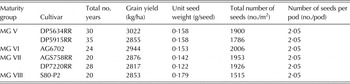
The model performance tests consisted of planting date, ranging from 7 May to 29 June, total amount of irrigation applied during the trials, grain yield (HWAM, kg/ha, with 13% moisture content), maturity date (MDAP, calendar days) and unit weight at maturity (HWUM, mg). Grain yield was corrected to 0% moisture content, as the crop models predict yield on a dry weight basis. Besides these variables, the number of seeds per pod was assumed to be 2·05, which was obtained from the provided DSSAT soybean cultivar file. The total number of seeds could then be calculated as maturity yield/unit seed weight (Table 1).
Average of observed data from the University of Georgia College of Agricultural and Environmental Sciences Statewide Variety Testing programme

Model calibration and evaluation procedure
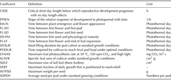
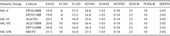
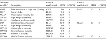
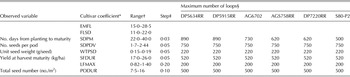
The CSM-CROPGRO-Soybean model defines 15 cultivar coefficients (Table 2) to simulate daily growth and development in response to weather and soil conditions and crop management (Guerra et al. Reference Guerra, Hoogenboom, Garcia y Garcia, Banterng and Beasley2008). The general calibration procedures and definition of model input parameters were similar to the studies conducted by Soler et al. (Reference Soler, Sentelhas and Hoogenboom2007, Reference Soler, Maman, Zhang, Mason and Hoogenboom2008). Cultivar coefficients were calibrated using GENCALC, which starts with the initial coefficients that are extracted from the genotype file of DSSAT and selects the best value for each coefficient by evaluating the root mean square error (RMSE) between the simulated and observed variables (Hunt et al. Reference Hunt, Pararajasingham, Jones, Hoogenboom, Imamura and Ogoshi1993). For soybean, the values for the generic maturity groups are normally used as initial coefficients (Table 3). GENCALC was designed to search for the best value of coefficients in a limited range. The parameters STEP and LOOPS control its search range for each special cultivar coefficient by setting the change for each step, i.e. STEP, and the number of times GENCALC should change the values of a particular coefficient, i.e. LOOP (Table 4).
Definition for the cultivar coefficients of the CSM-CROPGRO-Soybean model that determine soybean growth, development and yield


Configuration of GENCALC for calibration of the soybean cultivar coefficients

* DSSAT code for the observed variables.
† The definitions of the cultivar coefficients are defined in Table 2.
‡ Change in the value for each coefficient for each step when using GENCALC for calibration.
§ Number of times the coefficients can change.
Model calibration started with selecting parameters. The soil fertility factor (SLPF) and several essential crop cultivar coefficients were selected first. The soil fertility factor is an input parameter for the crop models that affects the overall crop growth rate by modifying daily canopy photosynthesis and is attributed to soil fertility differences and soil-borne pests, such as nematodes (Mavromatis et al. Reference Mavromatis, Boote, Jones, Irmak, Shinde and Hoogenboom2001; Guerra et al. Reference Guerra, Hoogenboom, Garcia y Garcia, Banterng and Beasley2008). Normally, simulations with appropriate SLPF values would be close to the observations. A suitable SLPF should be determined first, prior to calibrating the cultivar coefficients. The adjustment of SLPF was conducted by comparing observed and simulated grain yield for each of the six locations. To determine the best value for SLPF for one location, all six cultivars for all years (2001–2008) at that location were used. The SLPF was modified manually with values ranging from 0·7 to 0·94 (Jones et al. Reference Jones, Boote, Hoogenboom, Jagtap and Wilkerson1989; Mavromatis et al. Reference Mavromatis, Boote, Jones, Irmak, Shinde and Hoogenboom2001) and the one that provided the lowest RMSE between simulated and observed yield was selected.
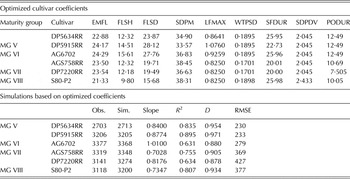
Although 15 cultivar coefficients were defined for simulations, because of the limited observed data that were available from the Statewide Variety Testing, only six candidate coefficients could be optimized with GENCALC. These included photothermal days from first seed to physiological maturity (SDPM), seed-filling duration for an individual pod cohort (SFDUR), seed size (WTPSD), maximum leaf photosynthetic rate (LFMAX), average number of seeds per pod under standard growing conditions (SDPDV) and the time required for soybean to reach final pod load under optimal conditions (PODUR). In order to obtain a reasonable simulation for the number of days to maturity, the photothermal days from first flower to first pod (FLSH), from first flower to first seed (FLSD), and the photothermal time from emergence to flower appearance (EMFL) were manually adjusted when running GENCALC for SDPM. The best value for each cultivar coefficient could be obtained only within the range that consisted of the maximum and minimum value for that coefficient in the cultivar file (Table 5).
The minimum and maximum values of each candidate coefficient and the set of STEP and LOOPS as used in GENCALC. The observed variables and corresponding cultivar coefficients are the same as in Table 4

* See Table 2 for the definitions of the cultivar coefficients.
† Minimum and maximum value for each cultivar coefficient.
‡ Change in coefficients for each step during the calibration process.
§ The maximum number of loops cannot exceed this value to avoid a search beyond the range.
Cultivar coefficient calibration
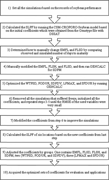
The SLPF was adjusted first to obtain reasonable simulations in grain yield, and then the cultivar coefficients were calibrated. Since an accurate simulation for the number of days to maturity is essential, candidate coefficients started with EMFL, FLSH, FLSD and SDPM, which are related to the number of days to maturity. CSM-CROPGRO-Soybean was run with a set of initial values and then a comparison was made between the simulated and observed number of days to maturity to determine the direction for manually changing EMFL and FLSD. The values of EMFL and FLSD were decreased when the simulated number of days to maturity was greater than the observed value, otherwise the values were increased. The changes were 0·5% for EMFL and 1·5% for FLSD. The FLSH was changed using the following equation:
 $$FLSH = {(FLSH/FLSD)_{MG}} \times FLS{D_{opt}}$$
where FLSD opt is the optimized value of FLSD based on GENCALC and (FLSH/FLSD)MG is the ratio of the general maturity group values for the specific coefficients (Mavromatis et al. Reference Mavromatis, Boote, Jones, Irmak, Shinde and Hoogenboom2001). GENCALC was run to search for the value of SDPM each time when EMFL and FLSD were changed. The set of EMFL, FLSD, FLSH and SDPM was selected when the simulated number of days to maturity matched the observed value.
After the calculation of the number of days to maturity, the next step was calculating the coefficients that determined grain yield. As with the rule for the above, the coefficients’ values with the smallest RMSE for each variable were selected. The corresponding variable for WTPSD was seed size, for PODUR was seed number, for SDPDV was seed number per pod, and for SFDUR and LFMAX was grain yield. The first set of calibrated coefficients could be obtained from this step and the simulations should be close to the observed values.
A check for the outliers of the simulations was performed based on the first set of coefficients from the above step. The years for which a freeze was simulated were removed from the simulations, as these data could lead to under-valuing of the genetic coefficients. All the candidate coefficients were initialized and the cultivar coefficients related to each observed variable were calculated again. The order was from the number of days to maturity to grain yield. A second set of coefficients was obtained based on the simulations in which a freeze did not occur. If the simulations and observations did not match well, the candidate cultivar coefficients could be manually adjusted; otherwise, the simulations proceeded directly to the next step.
Although the simulated variables performed fairly well based on the above-mentioned approach, improvements could be made by repeatedly adjusting the SLPF since it was calculated based on the initial values that were used for the cultivar coefficients. The SLPF was calculated again by minimizing the RMSE of grain yield based on the second set of coefficients. Because of the change of SLPF, cultivar coefficients were adjusted. This time the cultivar coefficients were not initialized, but they were modified based on the second set from the above procedure. The best set of optimized cultivar coefficients was then obtained.
The procedure for calibrating SLPF and the candidate cultivar coefficients is summarized in Fig. 1. The accuracy of the procedure for estimating the cultivar coefficients was also evaluated by the coefficient of determination (R 2) from function (2) and index of agreement (d) from function (3). Both R 2 and d ranged from 0 to 1; a best fit requires that they are 1.
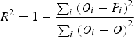 $${R^2} = 1 - \displaystyle{{\mathop \sum \nolimits_i {{({O_i} - {P_i})}^2}} \over {\mathop \sum \nolimits_i {{({O_i} - \bar O)}^2}}}$$
where O i is the ith observation, P i is the i th simulation and is the mean of all observations.
 $$d = 1 - \left[ {\displaystyle{{\mathop \sum \nolimits_{i = 1}^n {{({P_i} - {O_i})}^2}} \over {\mathop \sum \nolimits_{i = 1}^n {{\left( {\left\vert {P_i^{\prime}} \right\vert - \left\vert {O_i^{\prime}} \right\vert} \right)}^2}}}} \right],\quad 0 \le d \le 1$$
where n is the number of observations, P i is the predicted value for the i th measurement, O i is the observed value for the i th measurement,  $P_i^{\prime} = {P_i} - \bar O$,
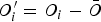 $O_i^{\prime} = {O_i} - \bar O$, where
 $\bar O$ is the mean of all observations
Procedure for model calibration based on the number of days to maturity, seed size and yield.

Evaluation of cultivar coefficients
After calibration of the cultivar coefficients, a comparison between observed and simulated grain yield was performed based on the best coefficients that were obtained during calibration. Evaluation was conducted using the observed values that were obtained from the experiments that were conducted during the years 2002, 2004, 2006 and 2008.
Soybean yield prediction
The CSM-CROPGRO-Soybean model was used to predict the number of days to maturity and grain yield for the cultivars DP5634RR, DP5915RR, AGS6702, AG758RR, DP7220RR and S80-P2, for the period of 1958 to 2008 (reference simulations), and for climate change projections for 2011, 2020, 2030, 2040 and 2050 for rainfed conditions for Calhoun, Williamson, Midville, Plains and Tifton. The inputs for the CSM-CROPGRO-Soybean, including soil profiles, plant population, row spacing and planting depth at each location, were the same as the values used for model calibration for the same location. No irrigation was applied and no nitrogen fertilizer was needed, as soybean is a leguminous crop that fixes nitrogen.
The weather inputs for the reference simulations were the corresponding observed daily weather data, including precipitation, minimum temperature, maximum temperature and solar radiation from 1958 to 2008. Long-term observed weather data from 1958 to 2008 obtained from the National Climatic Data Center (NCDC) were used as the reference data. Because this data set did not include solar radiation, the data from 1958 to 2008 (reference years) were provided by Garcia y Garcia & Hoogenboom (Reference Garcia y Garcia and Hoogenboom2005), who used the Weather Generator for Solar Radiation (WGENR) to generate solar radiation values based on a multivariate stochastic process using minimum and maximum temperature and precipitation as inputs.
The weather inputs for simulations from 2011 to 2050 were the reference weather data that were modified based on future climate patterns obtained from SimCLIM. The marker scenario A1B, which represents a medium level of greenhouse gas emissions, from the Special Report on Emissions Scenarios (SRES, Nakicenovic & Swart Reference Nakicenovic and Swart2000) was selected. Based on the recommendation of Hulme et al. (Reference Hulme, Wigley, Barrow, Raper, Centella, Smith and Chipanshi2000), at least three GCMs should be selected in case the prediction is limited to a narrow representation of future climate. Therefore, three commonly used GCMs were selected for the present study, i.e. the UK Meteorological Office's Hadley Centre Coupled Model version 3 (UKMO-HadCM3 (UKMO), the Commonwealth Scientific and Industrial Research Organisation's model CSIRO-Mk3.0 (CSIRO), and the Geophysical Fluid Dynamics Laboratory's model GFDL-CM2.1 (GFDL). Three resulting projections for monthly average temperature and precipitation for 2011, 2020, 2030, 2040 and 2050 for Calhoun, Williamson, Midville, Plains and Tifton were generated with SimCLIM. The reference daily precipitation and minimum and maximum temperature were modified based on the monthly climate change as calculated by SimCLIM and were used as input in the soybean simulations for the climate change projections for 2011, 2020, 2030, 2040 and 2050.
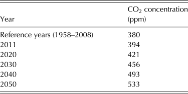
The CO2 concentrations for the projected years 2011, 2020, 2030, 2040 and 2050 were obtained from the database for SimCLIM (Table 6). To evaluate potential options for adaptation to climate change, simulations were run for all six varieties and four planting dates, i.e. 5, 15 and 25 May and 5 June. For each of the five locations, projection years and GCMs, the number of days to maturity and grain yield were analysed.
CO2 concentration for scenario A1B for future climate projections
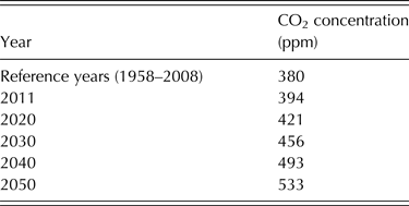
Source: SimCLIM version 2.1.7.0.
RESULTS
Soil fertility adjustment
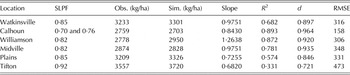
The optimized value for the Soil Fertility Factor (SLPF) was 0·85 for Watkinsville, 0·76 and 0·70 for Calhoun (where the experiment was conducted at two locations with different soil types), 0·82 for Williamson, 0·82 for Midville, 0·85 for Plains and 0·92 for Tifton (Table 7). The simulated yield was based on the optimized values for SLPF for each site using statistical analysis. The slope of the regression ranged from 0·682 to 1·264; the coefficient of determination, R 2, ranged from 0·33 to 0·89, the value for d ranged from 0·72 to 0·97 and the RMSE compares to the observed yield ranged from 158 to 473 kg/ha. For the linear regression of simulated v. observed yield, a slope close to 1 and a value for R 2 close to 1 mean a good fit. A lower RMSE also means a better fit. Calhoun had the lowest RMSE for yield but the crop model under-estimated yield by c. 56 kg/ha. Grain yield was also under-estimated by c. 32 kg/ha for Watkinsville and 46 kg/ha for Midville. The grain yield was over-estimated at Tifton, Plains and Williamson by c. 150 kg/ha. For Tifton the R 2 (0·33) and d (0·72) were the lowest when compared to all locations, while the RMSE (473 kg/ha) was the highest. The SLPF values for the six locations were different from the values determined by Mavromatis et al. (Reference Mavromatis, Boote, Jones, Irmak, Shinde and Hoogenboom2001). However, the RMSE between simulations and observations from the present study ranged from 156 to 227 kg/ha and were less than those reported by Mavromatis et al. (Reference Mavromatis, Boote, Jones, Irmak, Shinde and Hoogenboom2001) for Calhoun, Williamson and Midville, showing improved calibration procedures.
Estimation of the soil fertility factor (SLPF) for six locations and observed (Obs.) and simulated (Sim.) grain yield. Statistics include slope of regression; coefficient of determination (R2); index of agreement (d); and RMSE of simulated and observed yield

Cultivar coefficient calibration
The average yield for the six cultivars was estimated (Table 8) and showed that the difference between simulated and observed yield was <3%. The yield for DP5915RR and AG6702 was under-estimated by the crop model, but the difference was <10 kg/ha compared to the observed yield, 3300 kg/ha. The RMSEs of DP5634RR, DP5915RR and AG6702 ranged from 230 to 279 kg/ha, which were smaller than those for the other three cultivars, while the values for the slope of the regression equation ranged from 0·84 to 1·01 and were also close to 1. However, the values for R 2 and d showed that the optimized cultivar coefficients performed better for DP5634RR, DP5915RR and S80-P2 (R 2 = 0·8–0·9; d = 0·93–0·97) than for the other cultivars.
Optimized cultivar coefficients* and the average observed (Obs.) and simulated (Sim.) grain yield (kg/ha) for each cultivar. Statistics include slope of regression; coefficient of determination (R2); index of agreement (d); and root mean square error of simulated and observed yield (RMSE)

* See Table 2 for the definitions of the cultivar coefficients.
Cultivar DP5634RR had both the lowest observed and simulated grain yield among the six cultivars. Normally, if the values of the cultivar coefficients LFMAX, WTPSD, SFDUR, SDPDV and PODUR are smaller, the simulated yield should be lower for that cultivar. For example, the values of WTPSD, SFDUR, SDPDV and PODUR for DP5634RR and AG6702 were close, but the value for LFMAX for AG6702 (0·9259) was higher than for DP5634RR (0·8641). Cultivar DP5915RR had a higher LFMAX than DP5634RR, but the value for SFDUR for DP5915RR was much lower. The longer growing season for DP5915RR contributed to a higher yield at maturity. Therefore, the values for the cultivar coefficients EMFL, FLSD and SDPM, which determined the length of the soybean growing season, were higher for cultivar DP5915RR than for DP5634RR.
Crop model evaluation
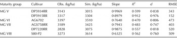
An evaluation for the performance of the optimized cultivar coefficients was conducted by comparing simulated and observed grain yield for the six locations (Table 9). The data collected from the soybean trials during the years 2002, 2004, 2006 and 2008 for the six locations were used for evaluation. The predicted grain yield for cultivars DP5634RR, DP5915RR, AG6702 and AGS758RR were <5% different from the observed yield, but there was an 8% difference for DP7220RR and 10% for S80-P2. Because the limited observations were used for calibration, the values of R 2 and d generally decreased and RMSE increased compared with model calibration for all cultivars except for DP5915RR. The comparison of the simulated and observed yield for DP5915RR had a slope of 0·8979, an R 2 of 0·912, a d of 0·976 and an RMSE of 152 kg/ha. For the remaining five cultivars, the comparison between simulated and observed yield had the following values: the slope ranged from 0·63 to 0·9969, the R 2 ranged from 0·47 to 0·562, the values for d ranged from 0·75 to 0·84 and the value for RMSE ranged from 343 to 520 kg/ha.
Model evaluation based on simulated (Sim.) and observed (Obs.) yield. Statistics include slope of regression; coefficient of determination (R2); index of agreement (d); and root mean square error of simulated and observed yield (RMSE)

Projections for monthly precipitation and mean temperature
The climate change patterns, including monthly precipitation and mean temperature for the projections for 2011, 2020, 2030, 2040 and 2050, were obtained using SimCLIM for Calhoun, Williamson, Midville, Plains and Tifton. These changes were defined with respect to the baseline for the period 1961–1990 and the values varied by location, month and the respective GCMs that were used. Monthly precipitation showed both a decrease and an increase from the baseline based on the three GCMs. In general, the projections based on the CSIRO GCM showed the largest change in precipitation for both the increase and decrease, while there was a moderate change in precipitation for the projections based on the GFDL GCM, and the smallest change in precipitation was for the projections based on the UKMO GCM. Monthly mean temperature increased from 2011 to 2050 compared with the baseline for the projections for all three GCMs. Although these changes in mean temperature were different for the individual months, the annual changes for the same year were similar among the three GCMs and did not vary by more than 0·5 °C. The difference among months for the same year became larger for both monthly precipitation and mean temperature as the projection years increased from 2011 to 2050.
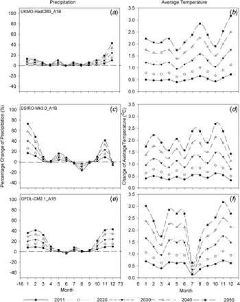
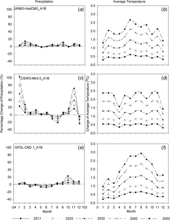
For Calhoun, the smallest change in monthly precipitation from the baseline was 0% for June for both the 2011 and 2050 projections (Fig. 2). The largest increase was 10% for 2011 and 43% for 2050 for December based on the UKMO GCM, while the increases for the remaining months were no more than 4% for 2011 and 19% for 2050. An extreme change occurred for August and January based on the CSIRO GCM, which was −4% for 2011 and −16% for 2050 for August and 17% for 2011 and 73% for 2050 for January. The decrease in precipitation for July, September and December was −1% for 2011, and ranged from −2 to −6% for 2050 based on the CSIRO GCM. For the GFDL GCM, the smallest change in precipitation was −1% for 2011 and −3% for 2050 for June, the largest change was 10% for 2011 and 43% for 2050 for December, and the change for April to September was <2% for 2011 and <10% for 2050.
Changes in monthly precipitation (%) and mean temperature (°C) as projected for 2011, 2020, 2030, 2040 and 2050 based on scenario A1B for three GCMs compared to the baseline data for the period 1961–1990 for Calhoun, Georgia. Precipitation (a) and temperature (b) for UKMO-HadCM3, precipitation (c) and temperature (d) for CSIRO-Mk3.0, and precipitation (e) and temperature (f) for GFDL-CM2.1. Precipitation change is in percentage and temperature is the difference in °C.

For Calhoun, the monthly mean temperature projections based on the three GCMs were somewhat different from the change in monthly precipitation (Fig. 2). For the UKMO GCM, the increase in temperature varied from 0·4 °C for May to 0·72 °C for December for 2011, and from 1·74 °C for May to 3·17 °C for December for 2050. For the CSIRO GCM, the increase in temperature varied from 0·32 °C for December to 0·61 °C for October for 2011, and 1·43 °C for December to 2·69 °C for October for 2050. For the GFDL GCM, the increase in temperature varied from 0·14 °C for July to 0·72 °C for November for 2011, and from 0·63 °C for July to 3·17 °C for November for 2050. When comparing the three GCMs, the change in monthly mean temperature based on the CSIRO GCM was the smallest compared to the other two GCMs.
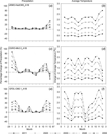
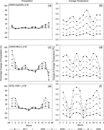
In general, the changes from baseline in monthly precipitation and mean temperature for Williamson for the projections for 2011 to 2050 were similar to those for Calhoun, with a few exceptions (Fig. 3). For the CSRIO GCM, the precipitation projection for March and April was close to 0% for the 2011 to 2050 projections, while for September it increased from about 3% for 2011 to 11% for 2050, and it decreased for December from −6% for 2011 to −29% for 2050. For the GFDL GCM, the precipitation for June increased by c. 5% for 2011 and 24% for 2050, but for July there was no change. The temperature change for August based on the UKMO GCM increased from 0·22 °C for 2011 to 2·22 °C for 2050, while for December it increased from 0·65 °C for 2011 to 2·85 °C for 2050.
Changes in monthly precipitation (%) and mean temperature (°C) as projected for 2011, 2020, 2030, 2040 and 2050 based on scenario A1B for three GCMs compared to the baseline data for the period 1961–1990 for Williamson, Georgia. Precipitation (a) and temperature (b) for UKMO-HadCM3, precipitation (c) and temperature (d) for CSIRO-Mk3.0, and precipitation (e) and temperature (f) for GFDL-CM2.1. Precipitation change is in percentage and temperature is the difference in °C.

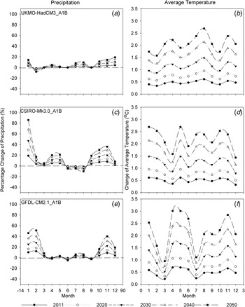
Midville showed a smaller increase in monthly precipitation from the baseline during the soybean growing season from 2011 to 2050, especially for the projections by the GFDL GCM when compared to Calhoun and Williamson (Fig. 4). Based on the three GCMs, the increase in monthly temperature for January and December was also smaller for Midville than for Calhoun and Williamson. For the UKMO GCM, the precipitation increase was ⩽14%, while there was a decrease in precipitation of −2% for both May and October. The CSIRO GCM did not show any change in precipitation for May. For the GFDL GCM the change in precipitation was <9% but October showed an increase of 5% for 2011 to 23% for 2050. The projections for March, May, June and July for 2050 showed a decrease in precipitation of almost −8%. Based on the UKMO GCM, the increase in temperature was c. 0·3 °C for 2011 and 2·7 °C for 2050 for January and December. The largest change in temperature based on the GFDL GCM occurred from May to October, and increased over time from 2·3 °C for 2011 to 2·93 °C for 2050.
Changes in monthly precipitation (%) and mean temperature (°C) as projected for 2011, 2020, 2030, 2040 and 2050 based on scenario A1B for three GCMs compared to the baseline data for the period 1961–1990 for Midville, Georgia. Precipitation (a) and temperature (b) for UKMO-HadCM3, precipitation (c) and temperature (d) for CSIRO-Mk3.0, and precipitation (e) and temperature (f) for GFDL-CM2.1. Precipitation change is in percentage and temperature is the difference in °C.

The change in monthly precipitation and mean temperature compared to the baseline for Plains from 2011 to 2050 was similar to Calhoun and Williamson (Fig. 5). However, for the UKMO GCM, precipitation decreased by c. −2% for February, while the GFDL GCM did not show a change in precipitation for April. The largest change in temperature based on the UKMO GCM was for August, which was 0·65 °C for 2011 and 2·85 °C for 2050.
Changes in monthly precipitation (%) and mean temperature (°C) as projected for 2011, 2020, 2030, 2040 and 2050 based on scenario A1B for three GCMs compared to the baseline data for the period 1961–1990 for Plains, Georgia. Precipitation (a) and temperature (b) for UKMO-HadCM3, precipitation (c) and temperature (d) for CSIRO-Mk3.0, and precipitation (e) and temperature (f) for GFDL-CM2.1. Precipitation change is in percentage and temperature is the difference in °C.

The change from baseline in monthly precipitation and mean temperature from 2011 to 2050 for Tifton was similar to Plains except for some details in precipitation (Fig. 6). For the UKMO GCM, the precipitation for February decreased by c. −2% for 2011 and −8% for 2050. For the CSIRO GCM, the precipitation decreased by −1% for 2011 and −5% for 2050 for June, while it increased by 2% for 2011 and 8% for 2050 for December. For the GFDL model, the decrease was −2% for April and −3% for September for 2050.
Changes in monthly precipitation (%) and mean temperature (°C) as projected for 2011, 2020, 2030, 2040 and 2050 based on scenario A1B for three GCMs compared to the baseline data for the period 1961–1990 for Tifton, Georgia. Precipitation (a) and temperature (b) for UKMO-HadCM3, precipitation (c) and temperature (d) for CSIRO-Mk3.0, and precipitation (e) and temperature (f) for GFDL-CM2.1. Precipitation change is in percentage and temperature is the difference in °C.

Soybean yield projections
The number of days to maturity and grain yield were simulated for the reference years and for the projections from 2011 to 2050 under rainfed conditions. Each of the projections contained simulations for 51 years. The following analysis is, therefore, based on the average of 51 years.
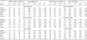
To determine the potential impact of climate change, the number of days to maturity and grain yield were first simulated for the 51 years of reference weather data for each location, maturity group and planting date (Table 10). The number of days to maturity for Calhoun was the longest, ranging from 134 to 182 days for all six cultivars, while Tifton had the shortest growing season, ranging from 120 to 163 days. Among the six studied cultivars, the growing season for AG6702, AGS758RR and S80-P2 was 3–22 days longer than the other three cultivars. Based on the four planting dates, the growing season of later-planted soybean was 6–16 days longer than earlier-planted soybean. For yield, Williamson and Plains had the highest yield, followed by Midville, while the yield in Calhoun and Tifton was 100–400 kg/ha less. Among the six cultivars, DP5915RR had the highest yield (1256–1636 kg/ha) and DP5634RR the lowest (1024–1385 kg/ha). Yield increased when the planting date was shifted from 5 to 25 May, while yield decreased when the planting date was shifted to 5 June for the cultivars AG6702, DP7220RR, AGS758RR and S80-P2. For the cultivars DP5634RR and DP5915RR, the yield increased when the planting date was shifted from 5 May to 5 June.
Simulated number of days to maturity and grain yield based on the reference weather data (1958–2008)s

PD: planting date.
Following the reference simulations, the climate change patterns for the three GCMs, i.e. UKMO, CSIRO and GFDL, as projected for 2011 to 2050 were applied to the reference historical data to predict future soybean yield. The potential impact of these climate patterns on the number of days to maturity and grain yield is discussed below with respect to the reference simulations. One normally would expect that an increase in the number of days to maturity would increase yield and a decrease in the number of days would cause a decrease in yield due to shorter grain filling duration.
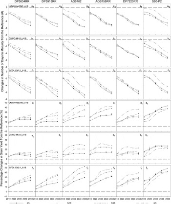
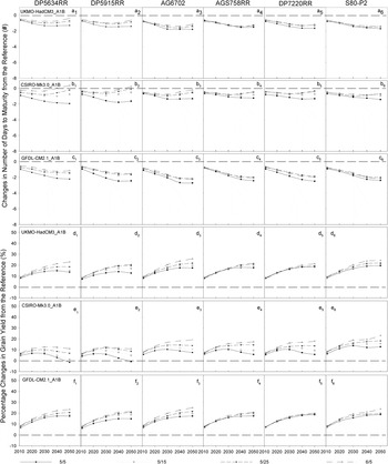
For Calhoun, the projected increase in mean temperature based on the three GCMs (Fig. 2) could cause soybean to develop faster, thereby decreasing the number of days to maturity for the projections from 2011 to 2050 for the cultivars that were analysed in the present study (Fig. 7). Over time, this situation could worsen. The decrease based on the GFDL GCM was larger than the UKMO and CSIRO GCMs. The number of days to maturity for the later-planted soybean for the projections from 2011 to 2050 decreased less than those of the earlier-planted soybean. The differences among the six cultivars studied were not great. Based on the UKMO and CSIRO GCMs, the decrease in the number of days to maturity for all cultivars ranged from −0·4 days for the 2010 projection to −3 days for the 2020 one, while there was a decrease from −1 to −6 days for the 2030, 2040 and 2050 projections. Based on the GFDL GCM, the decrease in the number of days to maturity was c. 1 to 2 days less than for the UKMO and CSIRO GCMs, especially for the 2040 and 2050 projections. The decrease in the number of days to maturity based on the 5 May planting date was c. 0·2–2 days more than those for 5 June. The cultivars AG6702 and S80-P2 planted on 5 June showed an increase of 0·1–0·4 days in the number of days to maturity for the 2010 and 2020 projections compared to the reference years.
Simulated number of days to maturity and yield of soybean for four planting dates for Calhoun, Georgia under projected climate change based on scenario A1B and GCMs UKMO-HadCM3, CSIRO-Mk3.0 and GFDL-CM2.1. X-axis is the projection for different years; Y-axis is changes in the number of days to maturity and yield. Panels a1–6, b1–6 and c1–6 are the change in number of days to maturity from the reference (1958–2008) under the projections of UKMO-HadCM3, CSIRO-Mk3.0 and GFDL-CM2.1 (#). Panels d1–6, e1–6 and f1–6 are for change in yield (%).

Grain yield for all cultivars increased for the 2011 to 2050 projections compared to the reference simulations (Fig. 7). The increase in yield with respect to the reference simulations was always larger for the 2050 projections than for the 2011 projections, partly due to the increase in precipitation (Fig. 2) and the increase in CO2 concentration (Table 2). Because the increase in precipitation during the soybean growing season (May to November) based on the UKMO and GFDL GCMs was larger than for the CSIRO GCM (Fig. 2), the increase in yield was larger for the projections based on the UKMO and GFDL GCMs. In general, the later-planted soybean showed a larger increase in yield than the earlier-planted soybean. However, the later-planted cultivar S80-P2 showed a smaller increase in yield than the earlier-planted soybean and this situation was worse for the 2011 than for the 2050 projections. This is possible because the longer growing season of the cultivar S80-P2 suffered frost damage. The increase in yield was 4–49% for all six cultivars that were studied based on the GCMs UKMO and GFDL, while the increase was 2–32% based on the GCM CSIRO. The increase in yield for the 2011 projection was 5–28% less than those for the 2050 projections. Later-planted soybean showed a 2–13% larger increase in yield than the earlier-planted soybean, while the later-planted S80-P2 cultivar had a 10–20% smaller increase in yield than the earlier-planted soybean. The cultivars AG6702, AGS758RR and S80-P2 showed a 5–20% larger increase in yield than the other cultivars.
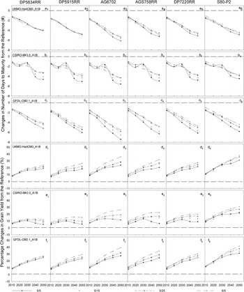
In general, the trend of the change in the number of days to maturity and yield for Williamson was similar for Calhoun (Fig. 8), but the differences among the four planting dates were less. The range for the decrease in the number of days to maturity was c. −1 day to −7·5 days based on the three GCMs. However, the decrease in number of days to maturity was lower for the 2030 projections, based on the CSIRO GCM, when soybean was planted later. The increase in yield was 7–42% based on the UKMO and GFDL GCMs, while the increase in yield ranged from 5 to 31% based on the CSIRO GCM. The later-planted cultivar S80-P2 had a larger increase in yield than earlier-planted soybean.
Simulated number of days to maturity and yield of soybean for four planting dates for Williamson, Georgia under projected climate change based on the scenario A1B and GCMs UKMO-HadCM3, CSIRO-Mk3.0 and GFDL-CM2.1. X-axis is the projection for different years; Y-axis is changes in the number of days to maturity and yield. Panels a1–6, b1–6 and c1–6 are the change in number of days to maturity from the reference (1958–2008) under the projections of UKMO-HadCM3, CSIRO-Mk3.0 and GFDL-CM2.1 (#). Panels d1–6, e1–6 and f1–6 are for change in yield (%).

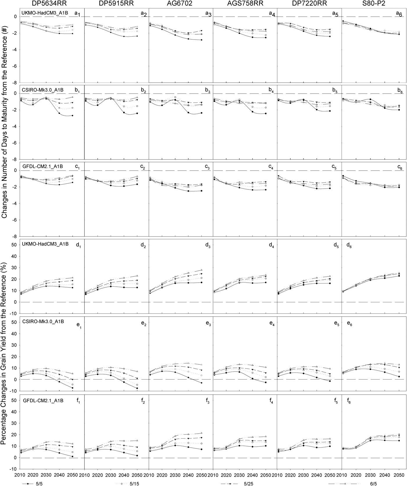
For Midville, the trend for the change in the number of days to maturity and yield was similar to Williamson (Fig. 9). However, there was not much difference for the decrease in the number of days to maturity for the 2011 to 2050 projections, which ranged from −0·6 to −2·9 days. Compared to Williamson, the increase in yield was less for Midville and ranged from 7 to 28% based on the UKMO GCM, from −8 to 14% based on the CSIRO GCM and from 1 to 21% based on the GFDL GCM. Because of the large decrease in precipitation that was projected for Midville, soybean that was planted earlier had lower yields for the 2040 and 2050 projections than the reference based on the CSIRO GCM, especially for cultivars DP5634RR and DP5915RR. The cultivars AG6702, AGS758RR and S80-P2 did not show a large increase in yield compared to the other cultivars for Midville, in contrast to the findings for Calhoun and Williamson.
Simulated number of days to maturity and yield of soybean for four planting dates for Midville, Georgia under projected climate change based on the scenario is A1B and GCMs UKMO-HadCM3, CSIRO-Mk3.0 and GFDL-CM2.1. X-axis is the projection for different years; Y-axis is changes in the number of days to maturity and yield. Panels a1–6, b1–6 and c1–6 are the change in number of days to maturity from the reference (1958–2008) under the projections of UKMO-HadCM3, CSIRO-Mk3.0 and GFDL-CM2.1 (#). Panels d1–6, e1–6 and f1–6 are for change in yield (%).
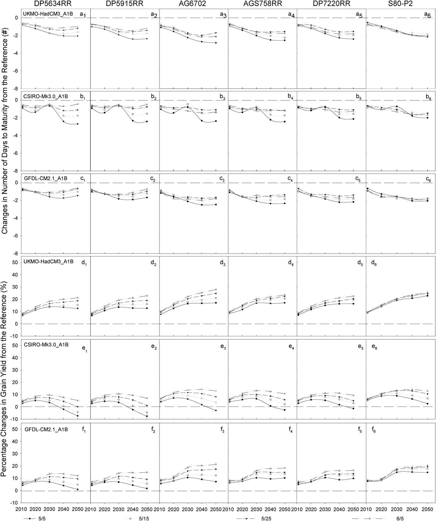
The change in the number of days to maturity and yield for Plains was similar to Midville, although some of the details were different (Fig. 10). The decrease in the number of days to maturity ranged from −0·4 to −4 days and the difference between the projections from 2011 to 2050 was larger than for Midville. There was no decrease in yield for the projections from 2011 to 2050 because the increase in precipitation for Plains was larger than for Midville. The increase in yield ranged from 6 to 24% based on the UKMO GCM, from 1 to 26% based on the CSIRO GCM and from 7 to 30% based on the GFDL GCM.
Simulated number of days to maturity and yield of soybean for four planting dates for Plains, Georgia under projected climate change based on the scenario A1B and GCMs UKMO-HadCM3, CSIRO-Mk3.0 and GFDL-CM2.1. X-axis is the projection for different years; Y-axis is changes in the number of days to maturity and yield. Panels a1–6, b1–6 and c1–6 are the change in number of days to maturity from the reference (1958–2008) under the projections of UKMO-HadCM3, CSIRO-Mk3.0 and GFDL-CM2.1 (#). Panels d1–6, e1–6 and f1–6 are for change in yield (%).

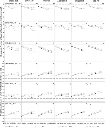
For Tifton, the decrease in number of days to maturity was much less compared to the other four locations and the number of days to maturity increased for the cultivars DP5634RR and DP5915RR, based on the CSIRO GCM for the projections for 2040 and 2050 compared to the reference years (Fig. 11). However, the increase in yield that was predicted was similar to Plains. There was a decrease in the number of days to maturity, ranging from −0·4 to −1·8 days for the UKMO GCM, from 0·4 to −2 days for the CSIRO GCM, and from −0·6 to −2·7 days for the GFDL GCM. The increase in yield ranged from 6 to 26% based on the UKMO and GFDL GCMs, but −1 to 23% based on the CSIRO GCM.
Simulated number of days to maturity and yield of soybean for four planting dates for Tifton, Georgia under projected climate change based on the scenario A1B and GCMs UKMO-HadCM3, CSIRO-Mk3.0 and GFDL-CM2.1. X-axis is the projection for different years; Y-axis is changes in the number of days to maturity and yield. Panels a1–6, b1–6 and c1–6 are the change in number of days to maturity from the reference (1958–2008) under the projections of UKMO-HadCM3, CSIRO-Mk3.0 and GFDL-CM2.1 (#). Panels d1–6, e1–6 and f1–6 are for change in yield (%).

DISCUSSION
All statistics showed that the calibrated CSM-CROPGRO-Soybean model could provide accurate simulations for the six selected cultivars. In general, the present study generated better results when compared with Mavromatis et al. (Reference Mavromatis, Boote, Jones, Irmak, Shinde and Hoogenboom2001), in which the RMSE for grain yield varied from 396 to 559 kg/ha.
The scenarios based on three GCMs showed differences in climate projections. In summary, the shorter soybean-growing season from 2011 to 2050 was caused by the increase in temperature; this observation is similar to the conclusion by Alexandrov & Hoogenboom (Reference Alexandrov and Hoogenboom2000). However, grain yield increased based on the climate scenarios of three GCMs for all five locations, except for the CSIRO GCM for Midville. Gain yield increased over time, partially due to the projected increase in precipitation during growing season except when a severe drought occurred, for instance for the CSIRO GCM for Midville. In addition, the increase in CO2 concentration also partially offset the negative effect of the projected increase in temperature. Because of the large decrease in precipitation during July, August and September for the CSIRO GCM for the 2011 to 2050 projections when compared to the baseline condition, the increase in yield base on the GCM CSRIO was less than the other two GCMs. All previous studies have stated that the soybean grain yield in south-eastern USA will decrease, even considering the impact of an increase in CO2 (Curry et al. Reference Curry, Jones, Boote, Peart, Allen, Pickering, Rosenzweig, Allen, Jones, Tsuji and Hildebrand1995; Alexandrov & Hoogenboom Reference Alexandrov and Hoogenboom2000; Carbone et al. Reference Carbone, Kiechle, Locke, Mearns, McDaniel and Downtown2003).
Some adaptation strategies can be provided for farmers to deal with the potential climate change based on the outcomes of the present study for the selected cultivars with different planting dates at multiple locations in Georgia. For the five locations where the simulations were conducted, Calhoun and Williamson were more suitable for rainfed soybean planting based on the projections from 2011 to 2050, followed by Plains and Tifton. On the other hand, Midville was less favourable for rainfed soybean production due to the projected decrease in precipitation. When other factors, such as the price of soybean, are acceptable, farmers could potentially expand their soybean production acreage especially at Calhoun and Williamson. In other words, soybean production at lower latitudes might shift to higher latitudes, especially for rainfed soybean planting. However, climate scenarios for Midville showed a decrease in precipitation, which means that soybean planted there might need additional irrigation to obtain a higher yield and to reduce the risks due to potential drought.
The simulations to determine the effect of planting date on grain yield showed that later-planted soybean had a higher yield than earlier-planted soybean. Farmers, therefore, should shift to a planting date around 5 June or possibly later, because the increase in mean temperature might cause potential heat and drought stress when planted earlier. However, because of the limitations of low temperatures at Calhoun, the planting date for cultivar S80-P2, which has a relatively longer growing season, could not be shifted to 5 June due to frost that occurred towards the end of the growing season. Therefore, the planting date can be later only if the growing season allows.
Finally, for the same environmental conditions, the cultivars AG6702, AGS758RR and S80-P2 had higher yields than the other four cultivars, especially for Calhoun and Williamson. However, the present study only evaluated the potential adaptation for recently released varieties. There is now an effort for breeding programmes to consider future climate change conditions as part of their evaluations (Ceccarelli et al. Reference Ceccarelli, Grando, Maatougui, Michael, Slash, Haghparast, Rahmanian, Taheri, Al-Yassin, Benbelkacem, Labdi, Mimoun and Nachit2010). Farmers should select soybean cultivars with heat and drought resistance for planting in the future to reduce the potential risks from climate change.
CONCLUSION
The results of the present study show that the genetic coefficient estimator, GENCALC, can be used as a tool for determining the cultivar coefficients for soybean using the limited data that are collected in state-wide variety trials. Based on the climate change projections from the three GCMs, the number of days to maturity decreased for all varieties and for all locations. The projected increase in temperature could benefit later-planted cultivars. However, the projected change in precipitation is the main cause for the change in grain yield. Overall, Calhoun, Williamson, Plains and Tifton are more suitable for soybean production for the next 40 years, while rainfed soybean production in Midville is less suitable due to the potential effects of climate change. One potential adaptation scenario for producers is to change the planting date to around 5 June in order to avoid heat stress and drought that can occur when planted earlier. Overall, the cultivars AG6702, AGS758RR and S80-P2 had the highest yield in the present study and could potentially be selected for rainfed production systems.
In the present study the potential impact of climate change for the baseline from 1961 to 1990 was determined for five locations in Georgia. However, it should be noted that a different baseline period or different locations could show different results due the complexity of the climate change projections.
This work was conducted under the auspices of the Southeast Climate Consortium (SECC; www.SEClimate.org) and supported by a partnership with the United States Department of Agriculture-Risk Management Agency (USDA-RMA), by grants from the US National Oceanic and Atmospheric Administration-Climate Programme Office (NOAA-CPO) and USDA National Institute of Food and Agriculture (NIFA) and by State and Federal funds allocated to Georgia Agricultural Experiment Stations Hatch project GEO01179. The dedicated support provided by Kim Evans is gratefully acknowledged.