1. Background
Methods for turbulent boundary layer wall layer control have generally focused on interacting in some form, with the low-speed wall streak structure first observed by Kline et al. (Reference Kline, Reynolds, Schraub and Runstadler1967). These methods are described in the comprehensive review by Corke & Thomas (Reference Corke and Thomas2018). One of the earliest approaches was ‘riblets’. Other active approaches include wall-normal suction and blowing, oscillating wall motion, uniform and oscillating body forces and lateral sublayer blowing. Riblets have been shown to yield a maximum drag reduction of approximately 8 %. Experiments with numerical simulations of oscillating walls (Baron & Quadrio Reference Baron and Quadrio1996; Trujillo, Bogard & Ball Reference Trujillo, Bogard and Ball1997; Dhanak & Si Reference Dhanak and Si1999; Choi & Clayton Reference Choi and Clayton2001; Choi, Chun-Xiao & Sung Reference Choi, Chun-Xiao and Sung2002) have predicted as much as a 40 % drag reduction, however, the power needed to oscillate the wall far exceeded the power savings due to the drag reduction. Simulations with an oscillating body force resembling a travelling wave (Du & Karniadakis Reference Du and Karniadakis2000, Reference Du and Karniadakis2002) predicted an  ${\textit{O}}(30)$ % drag reduction, suggesting a similar mechanism as an oscillating wall.
Recent active flow control experiments by Thomas et al. (Reference Thomas, Corke, Duong, Midya and Yates2019), Duong (Reference Duong2019) and Duong et al. (Reference Duong, Midya, Corke, Hussain and Thomas2019) have demonstrated unprecedented levels of viscous drag reduction of up to 78 % in turbulent boundary layers that produce a significant net power savings. The approach has focused on actively intervening with an autonomous cycle involving lift-up and break-up of coherent streamwise vorticity that is associated with the low-speed wall streak structure, that can account for as much as 70 % of the [ $uv$]-Reynolds stress (Corino & Brodkey Reference Corino and Brodkey1969), and whose frequency of occurrence scales linearly with the wall skin friction,
 $\tau _w$ (Kline et al. Reference Kline, Reynolds, Schraub and Runstadler1967).
The approach was motivated by simulations by Schoppa & Hussain (Reference Schoppa and Hussain1998) who observed that spanwise blowing in the wall layer of a turbulent channel flow resulted in a 50 % reduction in the viscous drag. They associated this effect with a lessening of the local spanwise mean flow distortion in the region flanking the low-speed wall streak structure. Later, Schoppa & Hussain (Reference Schoppa and Hussain2002) linked this result to control of ‘streak transient growth’, which they believe is responsible for the generation of new vorticity in the buffer layer, and on which the local wall-normal vorticity,  $\omega _y$, is a critical parameter. The link between the generation of streamwise vorticity in the buffer layer and skin friction drag has been provided by Kim (Reference Kim2011).
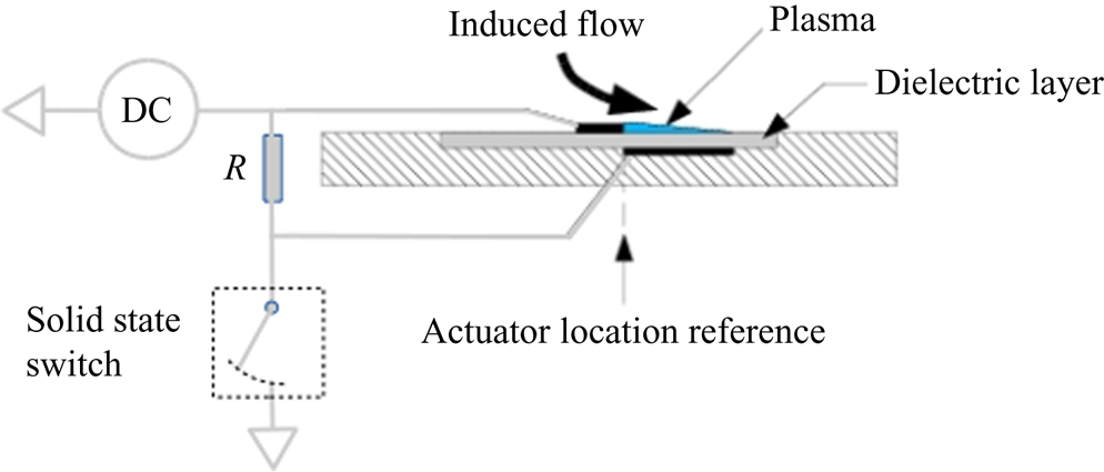
Our Thomas et al. (Reference Thomas, Corke, Duong, Midya and Yates2019), Duong (Reference Duong2019) and Duong et al. (Reference Duong, Midya, Corke, Hussain and Thomas2019), embodiment of this approach consists of an array of dielectric barrier discharge (DBD) plasma actuators that are designed to produce a spanwise velocity component in the wall layer of a turbulent boundary layer. The DBD plasma actuators consist of a pair of electrodes that are separated by a dielectric insulator. The electrodes are staggered as shown in the schematic in figure 1. One of the electrodes is exposed to the air. In the approach used for turbulent boundary drag reduction to minimize the plasma actuator input power, a pulsed-direct current (DC) power source was used. In this, the same DC potential is supplied to both electrodes. A fast-acting solid-state switch is then used to periodically ground the covered electrode for a short duration of  $10^{-5}$–
 $10^{-7}$ s. The alternating current (AC) that conducts through the dielectric during the short instant of the DC pulse causes the air to ionize. As indicated in figure 1, the ionized air forms on the surface of the dielectric over the covered electrode. The ionized air in the presence of the DC voltage potential produces a body force vector that acts on the neutral air in the direction of the electric field gradient. For the staggered electrode arrangement, the body force is directed away from the exposed electrode towards the covered electrode. This is indicated by the arrow labelled‘Induced flow’ in the figure. In the surface mounted configuration shown, this produces an effect that is similar to a tangential wall jet.
Schematic of pulsed-DC plasma actuator.

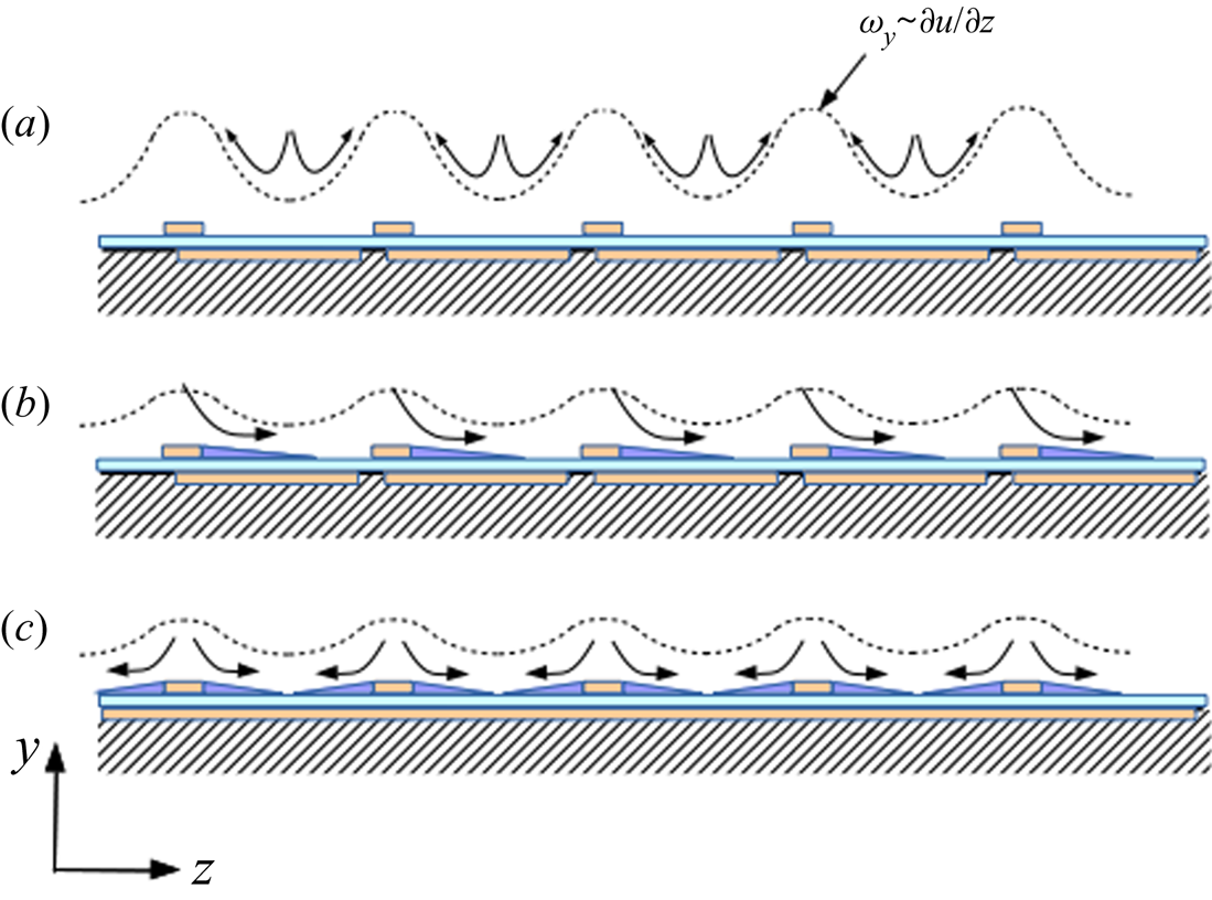
The approach used to produce a steady spanwise mean velocity component in the sublayer of a turbulent boundary layer is illustrated in figure 2. Figure 2(a) shows an idealized view of the spanwise variation of the local streamwise velocity that results from the pairs of counter-rotating streamwise vortices in the near-wall region of a turbulent boundary layer. This variation is the leading term in  $\omega _y$, which as mentioned, is the critical parameter in the streak transient growth mechanism of Schoppa & Hussain (Reference Schoppa and Hussain2002). Figure 2(b,c) shows two concepts that were investigated by Duong et al. (Reference Duong, Midya, Corke, Hussain and Thomas2019) and Thomas et al. (Reference Thomas, Corke, Duong, Midya and Yates2019). Both are based on flush, surface mounted plasma actuators. In concept (b), the plasma actuator was designed to produce a unidirectional spanwise near-wall velocity component (indicated by the curved arrows). In concept (c), the plasma actuators were designed to produce a series of spanwise opposed wall jets. Both have produced comparable drag-reduction levels.
Schematic of plasma flow control approach to reduce the mean flow distortion and thereby  $\omega _y$ produced by quasi-steady near-wall streamwise vortices associated with the wall ‘streak’ structure. (a) The baseline condition. (b) The uniform blowing configuration. (c) The counter blowing configuration.

The spanwise velocity component produced by either of the concepts shown in figure 2 are intended to produce a spanwise velocity component that ‘smooths’ the spanwise variation in the local streamwise velocity that was depicted in figure 2(a). As a result, it reduces  ${\partial u}/{\partial z}$, and hence the wall-normal vorticity,
 $\omega _y$, which is the critical parameter governing the streak transient growth mechanism (Schoppa & Hussain Reference Schoppa and Hussain2002). Our previous results (Duong Reference Duong2019; Duong et al. Reference Duong, Midya, Corke, Hussain and Thomas2019; Thomas et al. Reference Thomas, Corke, Duong, Midya and Yates2019) have indicated the importance of confining the spanwise blowing to the sub-layer and buffer layer in achieving drag reduction.
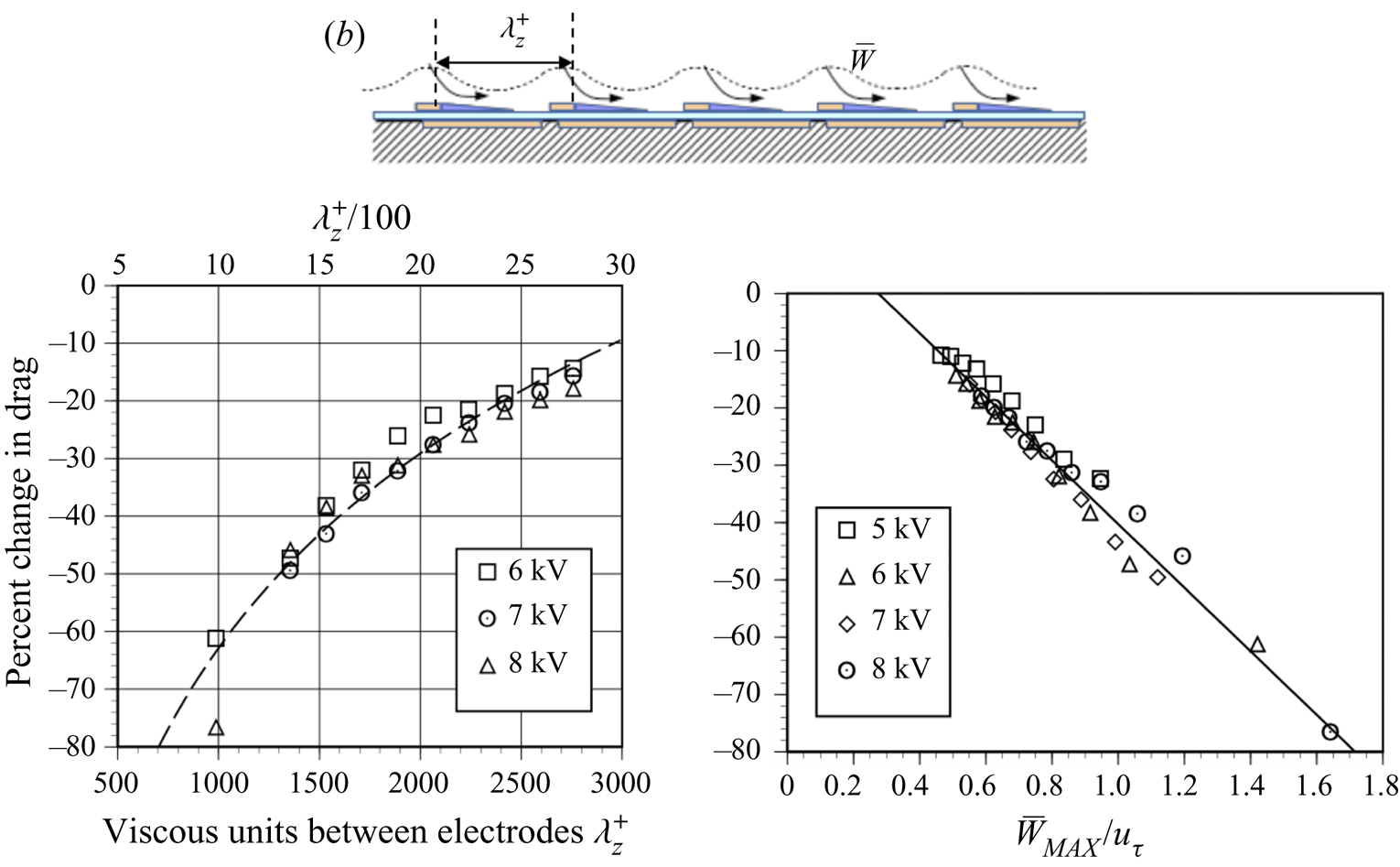
A significant result from the previous experiments (Duong Reference Duong2019; Duong et al. Reference Duong, Midya, Corke, Hussain and Thomas2019; Thomas et al. Reference Thomas, Corke, Duong, Midya and Yates2019) was the determination of boundary-layer-based scaling relations for the actuator design. For example, the degree of drag reduction strongly depends on the spanwise actuator spacing, which dictates the number of wall streak structures (nominally  $z^{+}\simeq 100$ apart) that are being simultaneously controlled. This is indicated in the left plot in figure 3, which shows the amount of drag reduction as a function of the spanwise surface electrode spacing
 $\lambda ^{+}_z=\lambda _z u_{\tau }/\nu$, defined in the illustration at the top of the figure. The upper abscissa in the plot corresponds to the average number of wall streak structures based on an average spacing of
 $z^{+}=100$ (Kline et al. Reference Kline, Reynolds, Schraub and Runstadler1967). The dashed curve is a logarithmic curve fit to the data. The results show a clear pattern of drag reduction with actuator spanwise spacing that scales with the inner-wall length scale,
 $z^{+}$. Using the same results, the percentage of drag reduction was put in terms of the mean spanwise velocity produced by the pulsed-DC plasma actuator normalized by the shear velocity of the baseline turbulent boundary layer. This indicates that the spanwise velocity needed to produce significant drag reduction need only be of the order of
 $u_{\tau }$.
Drag-reduction scaling from Thomas et al. (Reference Thomas, Corke, Duong, Midya and Yates2019) based on inner-wall layer spacing between electrodes,  $z^{+}$, and normalized spanwise blowing velocity,
 $\bar {W}/u_{\tau }$. Electrode arrangement is for unidirectional blowing arrangement (b) in figure 2.

It should be noted that for any given electrode spacing, over-forcing can lead to a drag increase. In the case of the results in figure 3, for the larger  $\lambda _z^{+}$ electrode spacing with the uniform blowing configuration (condition (b) in figure 2), this did not occur. In the experimental set-up described in § 2 with a
 $\lambda _z^{+}=300$, there was an optimum pulsed-DC voltage for maximum drag reduction.
With this background, the object of the present work is to document the characteristics of a turbulent boundary layer under a condition with spanwise wall blowing designed to produce significant viscous drag reduction. In addition, special emphasis will be placed on substantiating the proposed underlying mechanism for drag reduction resulting from a suppression of the turbulence producing events in the wall layer associated with the wall streak structure.
2. Experimental set-up
The experiments were performed in the Notre Dame Low-Speed Wind Tunnel at the Hessert Laboratory for Aerospace Research. The wind tunnel is a closed-return design with turbulence management that results in free-stream turbulence levels ( $u'_{rms}/U_{\infty }$, where rms is root mean square and U is the mean streamwise velocity component) of 0.05 %. The test section dimensions are 0.91 m square cross-section by 2.73 m long. The free-stream velocity range in the test section is from 1 to 50 m s
 $^{-1}$. The tunnel velocity and air temperature are respectively monitored by a Pitot-static probe and temperature sensor at the downstream location where the plasma actuator array was located. The test section is designed with three removable and fully interchangeable windows on all four sides. The windows can be replaced with panels that can be specifically designed for different experiments. One of these openings in the floor at the most downstream location of the test section was used to hold a force balance. Two sidewall openings at the force balance location were used to mount a three-dimensional (3-D) traversing mechanism that was used to locate two X hot-wire probes. Baseline turbulent boundary layer conditions at the leading edge of the force balance platen are reported in table 1. The free-stream velocity was chosen such that it would provide a thick canonical turbulent boundary layer that would maximize the spatial resolution for dual (X) hot-wire probe measurements, particularly within the sublayer.
Baseline turbulent boundary layer conditions at leading edge of force balance.

The turbulent boundary layer was developed on the floor of the wind tunnel test section. The boundary layer was thickened by placing a 2-D trip strip at the entrance to the test section. This was followed by uniformly spaced 2-D roughness elements that covered the first two thirds of the test section floor.
As presented in § 1, the plasma actuator array used in this study was the type shown in figure 2(b) and designed to produce a unidirectional spanwise velocity component near the wall. The spanwise spacing between the plasma actuators was  $\lambda _z=28$ mm. In terms of the turbulent boundary characteristics, this corresponded to
 $\lambda ^{+}_{z}=300$. Based on figure 3, this spacing was designed to produce significant drag reduction that was expected to result in tangible changes in the characteristics of the turbulent boundary that could identify underlying mechanisms.
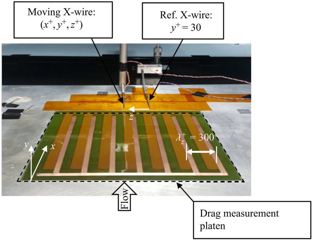
A photograph of the plasma actuator array mounted onto the surface of drag force measurement platen is shown in figure 4. The array is 22.9 cm by 22.9 cm square dimension that covered the whole surface of the platen. It consisted of 7 plasma actuators connected in parallel to the pulsed-DC power source. The electrodes consisted of 0.106 mm thick copper foil tape. In the photograph, the exposed electrodes are the narrow strips aligned in the flow direction. These are on the top surface of the dielectric material. The covered electrodes are the wider copper strips with one each per exposed electrode. These appear as a dull copper colour because they are being viewed through the translucent dielectric material layer. As shown in the schematic in figure 2, one side edge of the exposed and covered electrodes slightly overlap. The dielectric layer was a 22.9 cm by 22.9 cm by 0.1016 mm thick sheet of V2-quality muscovite mica. The underside of the mica was backed by a 0.0254 mm thick sheet of Kapton. The mica sheet was used because it has excellent dielectric properties that do not change over time when subjected to the ionized air. The complete plasma actuator array was bonded to a 25.4 mm thick Garolite sheet. The Garolite sheet was subsequently mounted to the force balance that was used to measure the viscous drag on the surface covered by the plasma actuator array.
Photograph showing plasma actuator array mounted onto the surface of the drag measurement platen, and pair of X hot-wire probes.

The force balance consisted of a recessed platen that rode on a pair of linear air bearings. The air bearings were aligned in the mean flow direction so that it was only sensitive to the streamwise component of the wall shear stress. The platen on which the plasma actuator array was mounted was adjustable at four points so that the flow-side surface of the array could be made flush to within  $\pm$0.254 mm of the test section floor. A cantilever style load cell with a maximum rated load of 0.5 N (51 g) was used to measure the total wall shear stress that acted over the area covered by the plasma actuator array. The load cell had an accuracy of 0.05 % of the maximum rate load which translated to a measurement uncertainty of 0.025 g. Drag force measurements consisted of sampling the load cell voltage over a 30 s interval to obtain an average value. The average voltage was converted to force using a predetermined linear voltage–force calibration. Direct drag measurements by Jasinski & Corke (Reference Jasinski and Corke2020) using the same force balance with a smooth platen surface over a range of momentum thickness Reynolds numbers matched the Coles–Fernholz relation (Baars et al. Reference Baars, Squire, Talluru, Abbassi, Hutchins and Marusic2016) to within 1 %.
Two dual (X) hot-wires were used to document the streamwise,  $u$, and wall-normal,
 $v$, velocity components within the boundary layer. These two X-wire probes are denoted in the photograph shown in figure 4. The hot-wires were operated in a constant temperature mode using a specially designed circuit that allowed the reference ground to float. This was essential for the hot-wire sensors to allow them to be placed in the ionized air stream directly downstream of and directly over the plasma actuator array. Although the air was weakly ionized (typically less than 1PPM weakly ionized gas Corke, Enloe & Wilkinson Reference Corke, Enloe and Wilkinson2010), charge build up on the hot-wires would otherwise lead to their immediate loss. Details of the anemometer circuit are given by Duong (Reference Duong2019).
One of the X-wire probes was mounted to the traversing mechanism and moved in 3-D space throughout the boundary layer. The motion resolution of the traversing mechanism in each direction was  $\varDelta _s=0.0254$ mm, which when normalized by turbulent boundary layer wall variables corresponded to
 $\varDelta _s u_{\tau }/\nu =0.27$.
The other X-wire probe was kept at a fixed location in the boundary layer. The streamwise location was 1 cm, or  $x^{+}=115$ downstream of the actuator array. The spanwise location aligned the X-wire probe with the edge of an exposed electrode facing the covered electrode of one of the plasma actuators in the array. This spanwise location of the fixed X-wire is defined as
 $z=0$. For a majority of the measurements, the wall-normal position of the fixed X-wire probe corresponded to
 $y^{+}=30$.
The voltage time series from the pair of X-wire probes was analogue frequency compensated to 8 kHz and anti-alias filtered at 10 kHz before being simultaneously digitally sampled at 20 kHz. The voltage time series were converted to velocity time series through the application of previously determined voltage–velocity calibrations for each hot-wire sensor. The two time series for each pair of X-wires were decomposed into the  $u$ and
 $v$ velocity components through previously determined angularity calibrations.
3. Results
3.1. Baseline and plasma actuator conditions
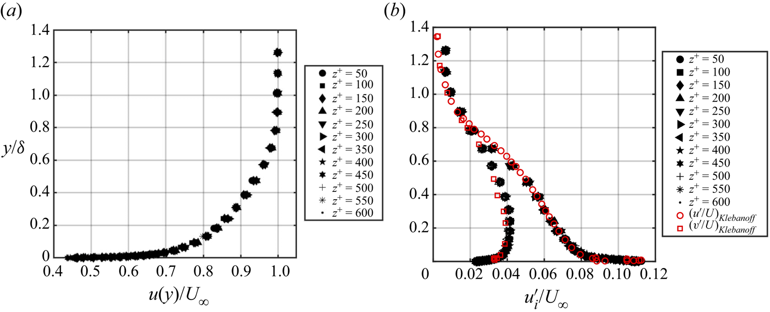
One of the first steps in the experiment was to verify that the mean characteristics of the boundary layer over the plasma actuator array was two-dimensional. This is documented in figure 5, which shows baseline mean velocity and turbulence intensity profiles measured over a range of  $z^{+}=600$, in increments of
 $z^{+}=50$. Physically, this corresponds to a span of 5.22 cm in increments of 4.25 mm, that spanned approximately two spanwise spacings between plasma actuators in the array. Recall that
 $z=0$ corresponds to the location of the fixed X hot-wire.
Mean velocity and  $u$ and
 $v$ turbulence intensity profiles for the baseline turbulent boundary layer.

Both the mean velocity and turbulence intensity profiles show excellent uniformity in the spanwise direction. Included in figure 5(b) is a comparison of the turbulence intensity profiles to that of Klebanoff (Reference Klebanoff1955). The excellent agreement certifies the canonical nature of the turbulent boundary layer in the present experiments.
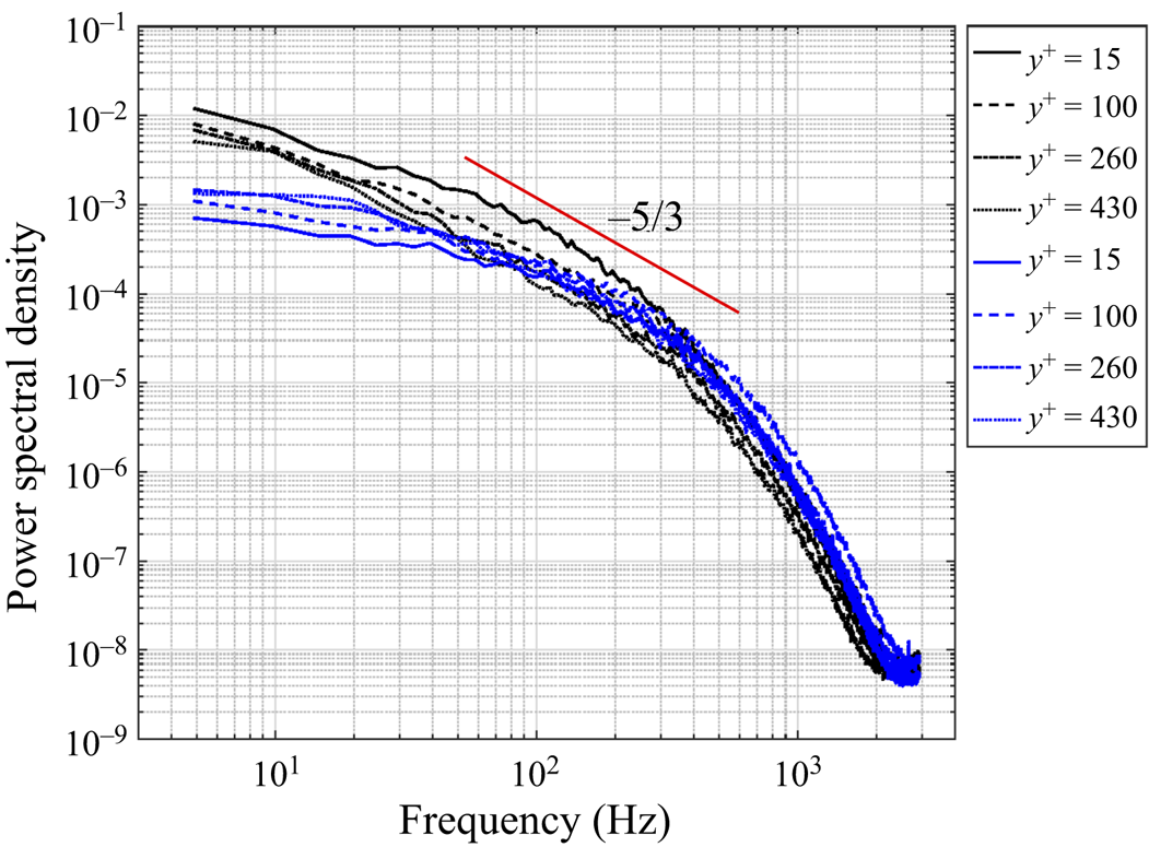
The canonical nature of the baseline turbulent boundary layer is further reflected in frequency spectra of the  $u'$ (shown in black) and
 $v'$ (shown in blue) velocity fluctuations for the baseline turbulent boundary layer that are shown in figure 6. These are presented for four different wall-normal distances of
 $y^{+}=15$, 100, 260 and 430 that encompass the location of peak turbulence fluctuations, the buffer layer and mean profile log–linear profile portion of the boundary layer. The spectra indicate a full distribution of scales including the important inertial sub-range over somewhat less than a full decade of frequency as is indicted by the line with the
 $-5/3$ slope.
Frequency spectra of the  $u$ (black) and
 $v$ (blue) velocity components for the baseline turbulent boundary layer.

The results to follow are based on a plasma array operating condition that was designed to produce a significant drag reduction that would highlight changes in the characteristics of the baseline turbulent boundary layer. The previous results documented by Duong (Reference Duong2019) and Thomas et al. (Reference Thomas, Corke, Duong, Midya and Yates2019) stressed the importance of confining the plasma actuator induced spanwise velocity component,  $\bar {W}$, to the sub- and buffer-layer regions of the turbulent boundary layer. Too large of an induced velocity was shown to lead to an increase in the viscous drag. For the pulsed-DC plasma actuator, the induced velocity is a function of the DC voltage, the time extent of the DC pulse, and the frequency of the DC pulses. Given a pulsing frequency, the time extent of the pulse can be represented as a duty corresponding to a per cent time of the DC pulse compared to the time period between pulses.
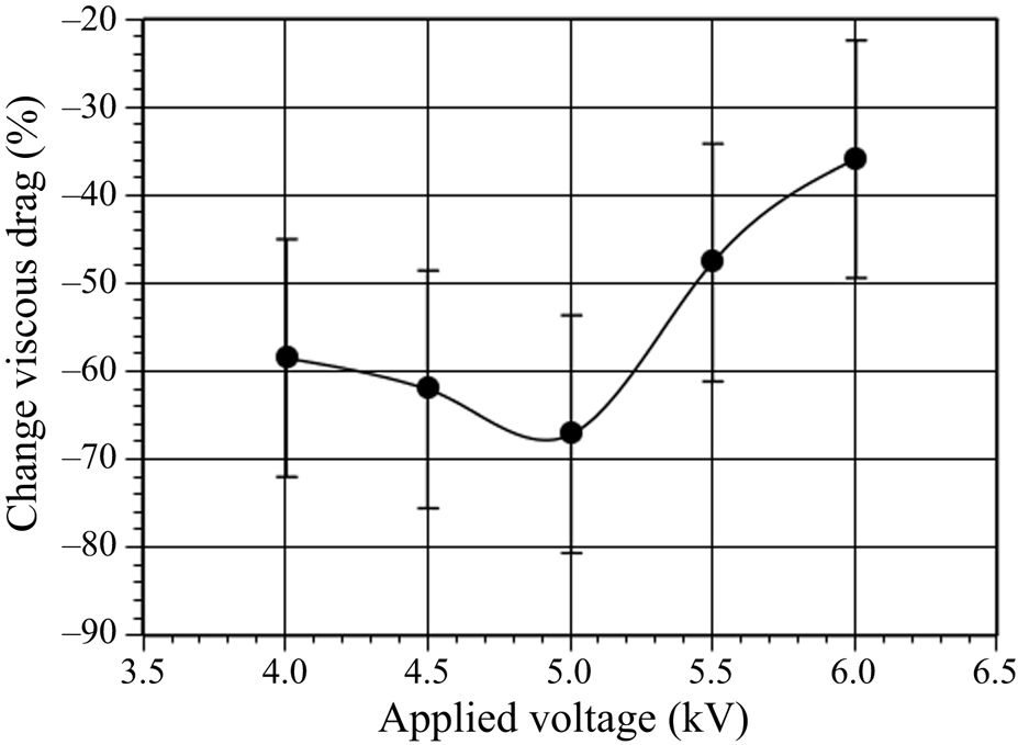
The first step in establishing the conditions for the plasma actuator in the present experiments was to determine the effect of its operation settings on the produced drag reduction. The approach used was to determine the optimum DC voltage for a fixed pulsing frequency of 500 Hz, and a pulse-width duty of 1 %. It is important to point out that the 500 Hz pulse frequency was not tied to any characteristic time scale of the baseline boundary layer. For comparison, the characteristic large-eddy frequency was 35 Hz and the near-wall characteristic frequency was 1.85 kHz.
Figure 7 shows the measured per cent drag reduction compared to the baseline turbulent boundary layer as a function of the plasma actuator DC voltage. Included in the figure are 95 % confidence-interval uncertainty bars. The result reveals a maximum drag reduction of approximately 68 % that occurred at a DC voltage of approximately 5 kV. This is the operating condition used for all of the results to follow, namely a DC voltage of 5 kV, pulsing frequency of 500 Hz and a pulse duty of 1 %.
Per cent drag reduction as a function of pulsed-DC actuator DC voltage at a pulsing frequency of 500 Hz and a pulse duty of 1 %.

The confidence bars in figure 7 reflect the combination of the accuracy of the load cell, and the standard deviation from multiple trials, typically 7 trials at each of the pulsed-DC voltages. In particular, for the voltage that produced the 68 % drag reduction, this corresponded to a reading of 0.136 g. The uncertainty in reading this low drag with a load cell with accuracy of 0.025 gis 18 %. The total uncertainty was the square root of the sum of squares of the measurement accuracy and the standard deviation of the repeated measurements, which was 24 %. The per cent drag reduction was then defined as the change in drag divided by the baseline drag  $\pm$ percentage, giving the total uncertainty which was
 $\pm$24 %. This large value is the result of having a low free-stream velocity, which was intended to help thicken the turbulent boundary layer (TBL) and thereby provide good spatial resolution for the
 $x$-wire measurements. However, the uncertainty was less than the drag-reduction trend with changing pulsed-DC voltage.
As a final point, the electrode spacing ( $\lambda _z^{+}=300$) was selected to produce a significant drag reduction in order to emphasize any changes in the turbulence characteristics. This is not the spacing that we recommend to achieve net drag reduction. At a comparable Mach number, Duong (Reference Duong2019) indicated the net power,
 $\Delta P/P_{in}$, break-even point at a
 $\lambda _z^{+} \simeq 1550$. At
 $\lambda _z^{+} \simeq 1800$, a
 $\Delta P/P_{in}=2.25$ was achieved. At higher Mach numbers, a
 $\lambda _z^{+} \simeq 1000$ is recommended (Duong Reference Duong2019), which at Mach 0.5, gave a
 $\Delta P/P_{in}\simeq 12$.
3.2. Turbulent boundary layer characteristics with drag reduction
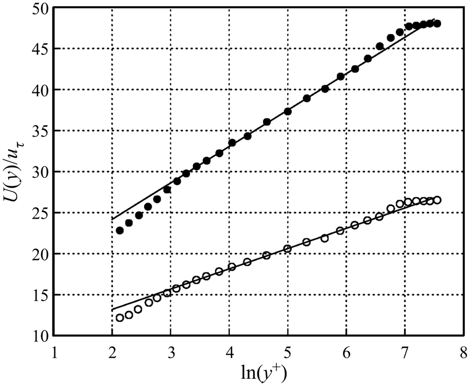
This section documents the characteristics of the turbulent boundary layer that resulted from the viscous drag reduction produced by the plasma actuator array under conditions listed in § 3.1. Figure 8 presents a comparison between the baseline and drag-reduced boundary layers of the inner-wall scaled mean velocity profiles. Here, as in subsequent results to follow,  $u_{\tau }$ used in the inner-wall scaling was determined by direct drag measurement. The straight line through the velocity profile data is a best fit to the logarithmic law of the wall. The drag-reduced boundary layer mean velocity profile retains a well-defined logarithmic region. However, the lower friction velocity in the drag-reduced boundary layer results in an expected shift in the log–linear fit additive constant. Also evident is an increase in the slope of the of the log–linear fit that translates into a decrease in the von Kármán coefficient,
 $\kappa$, from 0.405 found for the baseline boundary layer, to 0.225 found for the drag-reduced boundary layer. This is not surprising based on a recent study by Nagib & Chauhan (Reference Nagib and Chauhan2008) who examined a large set of turbulent boundary layers, and pipe and channel flows that revealed that the Karman coefficient is not universal, but exhibits a dependence on both pressure gradient and flow geometry. In our cases with drag reduction reported by Duong (Reference Duong2019) and Duong et al. (Reference Duong, Midya, Corke, Hussain and Thomas2019), the lower value of the Karman coefficient for the drag-reduced boundary layer was consistent with the Nagib & Chauhan (Reference Nagib and Chauhan2008) values obtained in canonical adverse pressure gradient turbulent boundary layers.
Inner-variable scaled mean velocity profiles for baseline (open symbol) and drag-reduced boundary layers (filled symbol) using  $u_{\tau }$ determined from direct drag measurement.

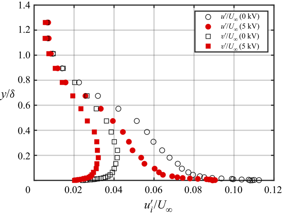
The effect of the drag reduction on the  $u$ and
 $v$ turbulence intensity profiles is presented in figure 9. The profiles for the baseline boundary layer correspond to the open symbols. Those for the drag-reduced boundary layer are shown by the filled symbols. These indicate a reduction in both components of turbulent velocity fluctuations that occurred with the drag reduction. As one might expect, the largest reduction in turbulent fluctuations occurred nearest to the wall. However, reductions in the turbulent fluctuations are evident out to the edge of the boundary layer.
Wall-normal profiles of  $u$ and
 $v$ turbulence intensity for baseline and drag-reduced boundary layers measured at
 $z^{+}=50$ location.

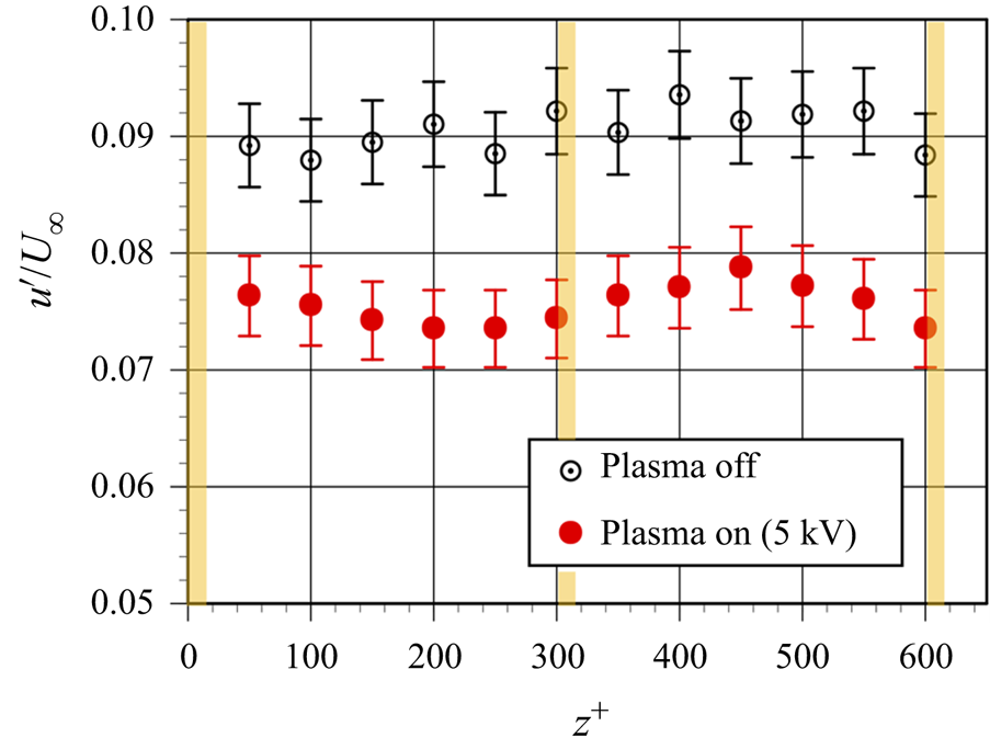
The turbulence intensity profiles shown in figure 9 were measured at the  $z^{+}=50$ spanwise location. Figure 10 illustrates that the effect was uniform across the full
 $z^{+}=600$ expanse of the measurements. This shows the
 $u$ turbulence intensity measured at
 $y^{+}=30$, for the baseline (open symbols) and drag-reduced boundary layers. The vertical lines indicate the locations of the plasma actuators in the array over that
 $z^{+}$ span. On a macro scale, figure 9 illustrates that within the experimental uncertainty, the reduction in the turbulent fluctuations that accompanied the drag reduction was uniform across the actuator array.
Spanwise distribution of  $u$ turbulence intensity measured at
 $y^{+}=30$ for baseline and drag-reduced boundary layers. Vertical lines indicate the plasma actuator locations in array.

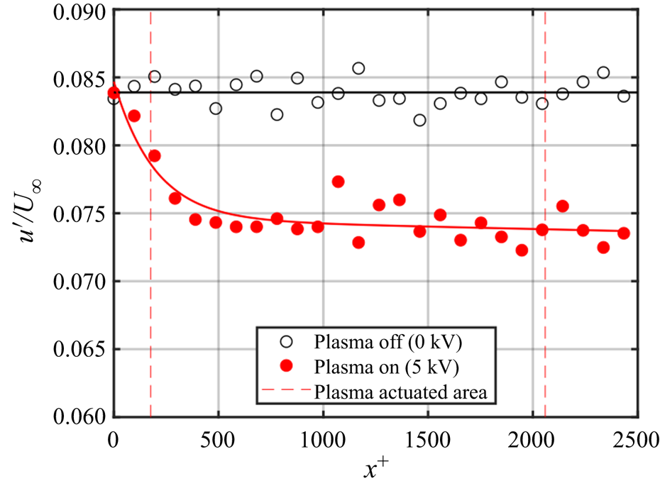
Having established that the drag-reduction results in a significant decrease in the velocity fluctuations near the wall, this decrease was used to establish the development length over the plasma actuator array needed to achieve the drag reduction. This was performed by moving a X hot-wire directly over the plasma actuator array along a line at a spanwise location of  $z^{+} = 50$ (50 wall units away from the edge a plasma actuator exposed electrode), and at a fixed height of
 $y^{+} = 30$. The result for the baseline and the drag-reduced turbulent boundary layers is shown in figure 11. The vertical dashed lines at
 $x^{+}=170$ and
 $x^{+}=2060$ mark the upstream and downstream edges of the plasma actuator array. For the baseline boundary layer (open symbols), the
 $u$ fluctuation level is constant over the full streamwise extent of the measurements. Based on the
 $u$ fluctuations, the effect of the plasma actuator array begins upstream of the array and reaches steady state at approximately
 $x^{+}=300$ from the array leading edge. These levels remain nearly constant over the actuator array, and persist to the most downstream location which is
 $x^{+}=440$ beyond the downstream edge of the plasma actuator array. This is 3.8-times further downstream of the
 $x^{+}=115$ location of the previous wall-normal profiles, therefore measurements taken at
 $x^{+}=115$ downstream of the actuator array are representative of the steady state condition over the array.
Streamwise development of  $u$ fluctuations for baseline and drag-reduced turbulent boundary layers measured at a fixed spanwise location of
 $z^{+} = 50$ and height of
 $y^{+} = 30$.

As a further observation, based on the  $u'$ measurement at
 $y^{+}=30$ in figure 11, only the downstream 84 % of the boundary layer over the drag measurement platen is experiencing the full, steady state drag reduction. Therefore the value measured, which is based on the area-averaged drag force, is under-predicted. As a result, the actual steady state
 $u_{\tau }$ inferred from the drag measurement is slightly lower.
Figure 9 has established a reduction in the turbulence intensity values through most of the boundary layer when normalized by the free-stream velocity,  $U_{\infty }$. One of the questions is how turbulence intensity levels scale with inner-wall variables, specifically
 $u_{\tau }$. In order to seek to answer that, we consider the ratio of the streamwise velocity fluctuations of the drag-reduced and baseline boundary layers, that are each normalized by their respective
 $u_{\tau }$ values. This ratio is defined as
 $R^2_{u^\prime }$ where
 \begin{equation} R_{u^\prime}^2 = \left(\frac{(u^\prime/u_{\tau})_{5\ \textrm{kV}}}{(u^\prime/u_{\tau})_{0\ \textrm{kV}}}\right)^2, \end{equation}
and the subscripts 5 kV and 0 kV refer to the drag-reduced and baseline boundary layers, respectively.
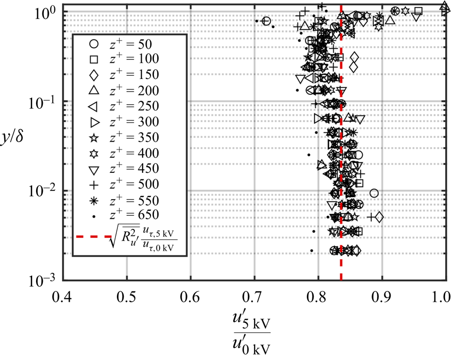
Values of  $R^2_{u^\prime }$ were calculated at every height in the boundary at all of the spanwise locations. The result is shown in figure 12. These profiles are observed to reasonably collapse. An average value based on the region from the wall up to the edge of the log layer, gave a value of
 $\overline {R_{u^\prime }^2}=1.86$. This is shown by the vertical dashed line in the plot.
Wall-normal variation in  $R^2$ given by (3.1) using
 $u^\prime$ turbulence intensity profiles of the baseline (0 kV) and drag-reduced (5 kV) boundary layers at all of the spanwise measurement locations. The vertical dashed line corresponds to
 $\overline {R_{u^\prime }^2}=1.86$.

Rewriting (3.1) as
 \begin{equation} R_{u^\prime}^2 = \left(\frac{u_{\tau,0\ \textrm{kV}} }{u_{\tau,5\ \textrm{kV}}}\right)^2 \left(\frac{u^\prime_{5\ \textrm{kV}}} {u^\prime_{0\ \textrm{kV}}}\right)^2 \end{equation}
separates out the ratio of the wall shear velocities for the baseline (0 kV) and drag-reduced (5 kV) boundary layers, which is known from direct drag measurement, and which
 \begin{equation} \left(\frac{u_{\tau,0\ \textrm{kV}}}{u_{\tau,5\ \textrm{kV}}}\right)^2=2.56, \end{equation}
so that
 \begin{equation} R_{u^\prime}^2 = 2.56 \left(\frac{u^\prime_{5\ \textrm{kV}}}{u^\prime_{0\ \textrm{kV}}}\right)^2 = 1.86. \end{equation}
In order for (3.4) to hold,
 \begin{equation} \left(\frac{u^\prime_{5\ \textrm{kV}}}{u^\prime_{0\ \textrm{kV}}}\right)^2 = 0.73 \quad \mbox{or}\quad \left(\frac{u^\prime_{5\ \textrm{kV}}}{u^\prime_{0\ \textrm{kV}}}\right) = 0.85. \end{equation}
As a check, the ratio of the  $u^\prime$ turbulence intensity between the drag-reduced (5 kV) and baseline (0 kV) boundary layers is plotted in figure 13. This again includes every height in the boundary layer at all of the spanwise locations measured. Again the profiles are observed to reasonably collapse. Taking an average based on the region from the wall to the edge of the log layer gives
 $\overline {(u^\prime _{5\ \textrm {kV}}/u^\prime _{0\ \textrm {kV}})} = 0.84$. The difference from the value in (3.5) is within the uncertainty of the measurements. A similar approach for the
 $v^\prime$ turbulence intensity measurements gave
 $\overline {(v^\prime _{5\ \textrm {kV}}/v^\prime _{0\ \textrm {kV}})} = 0.78$. Thus the method of drag reduction had a larger impact on reducing the
 $v^\prime$ turbulence intensity than on reducing the
 $u^\prime$ turbulence intensity. This is not surprising given that the
 $v^\prime$ fluctuations depend on the energy transfer from the reduced
 $u^\prime$ fluctuations via pressure strain rate terms.
Ratio of  $u^\prime$ turbulence intensity between baseline (0 kV) and drag-reduced (5 kV) boundary layers at all of the spanwise measurement locations. The vertical dashed line corresponds to
 $\overline {(u^\prime _{5\ \textrm {kV}}/u^\prime _{0\ \textrm {kV}})} = 0.84$.

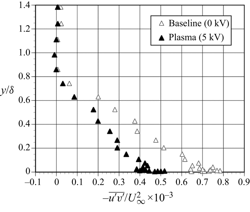
A comparison of wall-normal profiles of the normalized Reynolds stress,  $-\overline {u^\prime v^\prime }/U_\infty ^2$, for the baseline and drag-reduced boundary layers is shown in figure 14. Following the previous results, this is based on measurements taken at
 $x^{+}=115$ downstream of the plasma actuator array. As was the case for the normal stresses, the [
 $u^\prime v^\prime$]-Reynolds stress in the drag-reduced boundary layer is significantly lower compared to the baseline condition. In the near-wall region, the [
 $uv$]-Reynolds stress was reduced by approximately 40 %. Similar to the
 $u^\prime$ and
 $v^\prime$ turbulence intensity profiles that were shown in figure 9, the reduction in
 $u^\prime v^\prime$-Reynolds stress occurred throughout the lower 80 % of the boundary layer. The following results are aimed at the source of this Reynolds stress reduction.
Wall-normal distributions of the normalized  $uv$-Reynolds stress for the baseline and drag-reduced boundary layers.

As previously stated, the underlying premise of the flow control approach was to intervene with an autonomous cycle of low-speed fluid lift-up and break-up that was associated with the low-speed wall streak structure (Kline et al. Reference Kline, Reynolds, Schraub and Runstadler1967), and accounted for as much as 70 % of the [ $u^\prime v^\prime$]-Reynolds stress (Corino & Brodkey Reference Corino and Brodkey1969). One approach pioneered by Lu & Willmarth (Reference Lu and Willmarth1973b), is a conditional sampling method that can quantify the contributions of different events within this cycle to the total [
 $\overline {u^\prime v^\prime }$]-Reynolds stress. This begins by partitioning [
 $u^\prime v^\prime$] time series into quadrants based on the sign (positive or negative) of
 $u'$ and
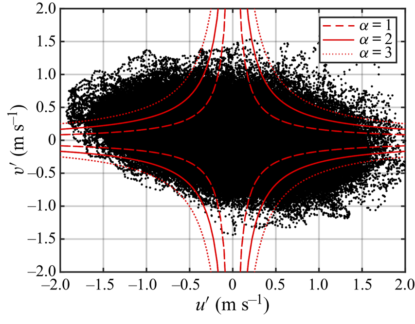
 $v'$. An example for the present experiment for the baseline boundary layer at
 $y^{+}=100$ is shown in figure 15. The dashed curves are hyperbolic functions used as threshold levels for conditioned statistics.
Sample [ $u^\prime v^\prime$] quadrant representation for baseline boundary layer at
 $y^{+} = 100$. Dashed curves are hyperbolic functions used as threshold levels for conditional statistics.

The two events that are most commonly quantified through the quadrant splitting method are ejection and sweep events, also referred to as Q2 and Q4 events, respectively. With reference to figure 15, Q2 events occur in the second quadrant where  $u'(t) < 0$ and
 $v'(t) > 0$. The Q4 events occur in the fourth quadrant where
 $u'(t) > 0$ and
 $v('t) < 0$. Lu & Willmarth (Reference Lu and Willmarth1973b) showed that the Q2 and Q4 events were the largest contributors to the [
 $\overline {u^\prime v^\prime }$]-Reynolds stress production in turbulent boundary layers.
The curves shown in figure 15 define hyperbolic ‘holes’ defined as
 \begin{equation} |u^\prime v^\prime| = \alpha \sqrt{\overline{u^{\prime 2}}}\sqrt{\overline{v^{\prime 2}}}, \end{equation}
where  $\alpha$ is a threshold level, shown as 1, 2 and 3 in figure 15. The [
 $u^\prime v^\prime$] values within a hyperbolic ‘hole’ are below the threshold for counting ‘[
 $u^\prime v^\prime$]-events’, either ‘ejection’ (Q2) or ‘sweep’ (Q4) events.
The formulation of the quadrant contributions to the total [ $\overline {u^\prime v^\prime }$]-Reynolds stress is
 \begin{equation} \frac{\widehat{u^\prime v^\prime_i}}{\overline{u^\prime v^\prime}}=\frac{1}{\overline{u^\prime v^\prime}}\lim_{T\rightarrow \infty} \frac{1}{T}\int^T_0 u^\prime(t)v^\prime(t)S_i(t,\alpha)\,\textrm{d} t\quad (i=1,2,3,4), \end{equation}
where  $i$ denotes the quadrant, and
 $S_i$ is a discriminator for the different quadrants where
 \begin{equation}
S_i(t,\alpha) = \begin{cases} 1 & \text{if }
u^\prime(t) \text{ and } v^\prime(t) \text{ are in quadrant
} i \text{ and } |u^\prime(t)v^\prime(t)| >
\alpha\sqrt{\overline{u^{\prime
2}}}\sqrt{\overline{v^{\prime 2}}},\\ 0 & \text{otherwise}.
\end{cases}
\end{equation}
The contribution to the total [ $\overline {u^\prime v^\prime }$]-Reynolds stress from the hyperbolic ‘hole’ is the same except with discriminator
 $S_H$ so that
 \begin{equation} \frac{\widehat{u^\prime v^\prime_H}}{\overline{u^\prime v^\prime}}=\frac{1}{\overline{u^\prime v^\prime}}\lim_{T\rightarrow \infty} \frac{1}{T}\int^T_0 u^\prime(t)v^\prime(t)S_H(t,\alpha)\,\textrm{d} t\quad (i=1,2,3,4) \end{equation}
and
 \begin{equation}
S_H(t,\alpha) = \begin{cases} 1 & \text{if }
|u^\prime(t)v^\prime(t)| \leq
\alpha\sqrt{\overline{u^{\prime
2}}}\sqrt{\overline{v^{\prime 2}}},\\ 0 & \text{otherwise}.
\end{cases}
\end{equation}
Given these definitions, the total contributions to the [ $\overline {u^\prime v^\prime }$]-Reynolds stress including all four quadrants and the hyperbolic ‘hole’ is
 \begin{equation} \sum_{i=1}^4 = \frac{\widehat{u^\prime v^\prime_i}}{\overline{u^\prime v^\prime}} + \frac{\widehat{u^\prime v^\prime_H}}{\overline{u^\prime v^\prime}} = 1. \end{equation}
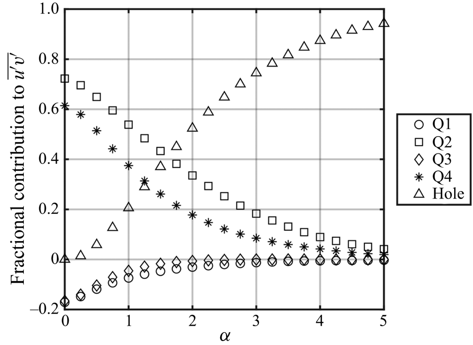
The contribution from each quadrant is a function of the ‘hole’ size, which is based on the parameter,  $\alpha$. This is illustrated in figure 16 for the baseline turbulent boundary layer at
 $y^{+}=15$, where the contributions to the [
 $\overline {u^\prime v^\prime }$]-Reynolds stress are plotted versus the ‘hole’ size parameter,
 $\alpha$. This indicates that the contributions of the Q1 and Q3 to the overall [
 $\overline {u^\prime v^\prime }$]-Reynolds stress is relatively small, and approaches zero asymptotically for large amplitude events,
 $\alpha > 2$. The largest contributions come from Q2 (ejection) and Q4 (sweep) events. Based on Lu & Willmarth (Reference Lu and Willmarth1973a), a value of
 $\alpha =4$ was chosen. This emphasizes the detection of large amplitude, dynamically significant events by the [
 $u^\prime v^\prime$] quadrant splitting approach.
Effect of hyperbolic ‘hole’ size parameter,  $\alpha$ on the quadrant contributions to [
 $\overline {u^\prime v^\prime }$]-Reynolds stress of baseline turbulent boundary layer at
 $y^{+}=15$.

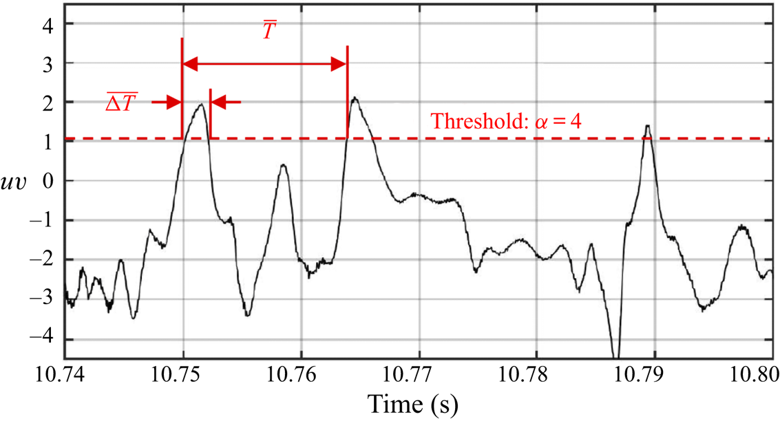
A first step in characterizing the difference between the baseline and drag-reduced turbulent boundary layers is to compile statistics on the average time between and duration of ejection (Q2) and sweep (Q4) events. An event is defined as [ $u^\prime v^\prime$] magnitude exceeding the threshold level defined by the hyperbolic curve with
 $\alpha =4$. This is illustrated in figure 17 which shows a sample [
 $u^\prime v^\prime$] time series with the represented
 $\alpha =4$ threshold shown by the horizontal dashed line. As illustrated, the duration of an event in the ith [
 $u^\prime v^\prime$] quadrant,
 $\overline {\Delta T_{i}}$, is defined to be the time between consecutive upward and downward crossings of the
 $\alpha =4$ threshold. The time between events in the ith [
 $u^\prime v^\prime$] quadrant,
 $\overline {T_{i}}$, is defined as the time between consecutive upward crossings of the
 $\alpha =4$ threshold. Following Antonia (Reference Antonia1972), the ratio,
 $\overline {\Delta T_{i}}/\overline {T_{i}}$, can be thought of as a parameter that is independent of convective speed and serves to characterize the dynamical significance of events occurring in the ith quadrant. Large values of
 $\overline {\Delta T_{i}}/\overline {T_{i}}$ would be associated with frequent and/or long duration events which would be considered most dynamically significant. Conversely, smaller values of
 $\overline {\Delta T_{i}}/\overline {T_{i}}$ would indicate less frequent and/or shorter duration events that are less dynamically significant.
Illustration defining event duration,  $\Delta \bar {T}$, and time between events,
 $\bar {T}$, for
 $u^\prime v^\prime$ time series with
 $\alpha =4$ threshold.

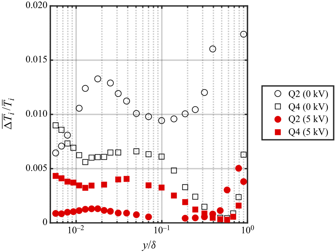
A comparison of the  $\overline {\Delta T_{i}}/\overline {T_{i}}$ ratio between the baseline and drag-reduced turbulent boundary layers for ejection (Q2) and sweep (Q4) events is presented in figure 18. These are shown at different heights from the wall, to the edge of the boundary layer. The open and closed symbols correspond to the baseline and drag-reduced boundary layers, respectively. Throughout the boundary layer, the ratios,
 $\overline {\Delta T_{i}}/\overline {T_{i}}$, corresponding to both ejection and sweep events are substantially reduced with drag reduction. The reduction in the dynamical significance of Q2 events is particularly significant. For example, at
 $y^{+}=15$ (
 $y/\delta \approx 0.01$) and
 $y^{+}=30$ (
 $y/\delta \approx 0.02$), the reduction in
 $\overline {\Delta T_{Q2}}/\overline {T_{Q2}}$ is 89 % and 90 %, respectively. This is fully consistent with the premise that the plasma-induced spanwise near-wall flow has reduced the cycle of low-speed fluid lift-up.
Comparison of the duration of events to the period of events occurring for a hyperbolic hole size of  $\alpha = 4$.

Very near the wall at  $y^{+}=8$ (
 $y/\delta \approx 0.008$),
 $\overline {\Delta T_{Q4}}/\overline {T_{Q4}}$ is reduced by 52 %. This indicates that wall-directed fluid motion giving rise to ‘splatting’ that has been shown associated with viscous drag (Canton et al. Reference Canton, Orlu, Chin, Hutchins, Monty and Schlatter2016; Yao et al. Reference Yao, Chen, Thomas and Hussain2017), has been strongly reduced. Farther from the wall at
 $y^{+}=15$ (
 $y/\delta \approx 0.01$) and
 $y^{+}=30$ (
 $y/\delta \approx 0.02$), the reduction in
 $\overline {\Delta T_{Q4}}/\overline {T_{Q4}}$ is 45 % and 43 %, respectively. It is clear from these observations that the dynamical significance of Q2 and Q4 Reynolds stress producing events has been greatly diminished in the drag-reduced boundary layer.
These results are further explored by presenting the ratios of the time between events,  $\overline {T_{i}}$, and the duration of events,
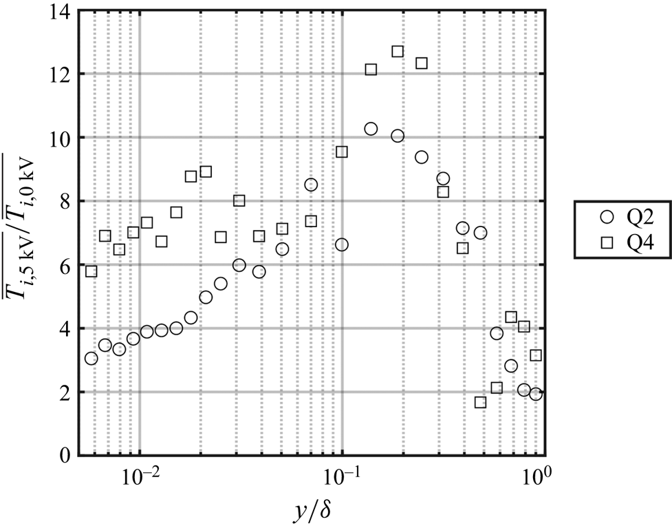
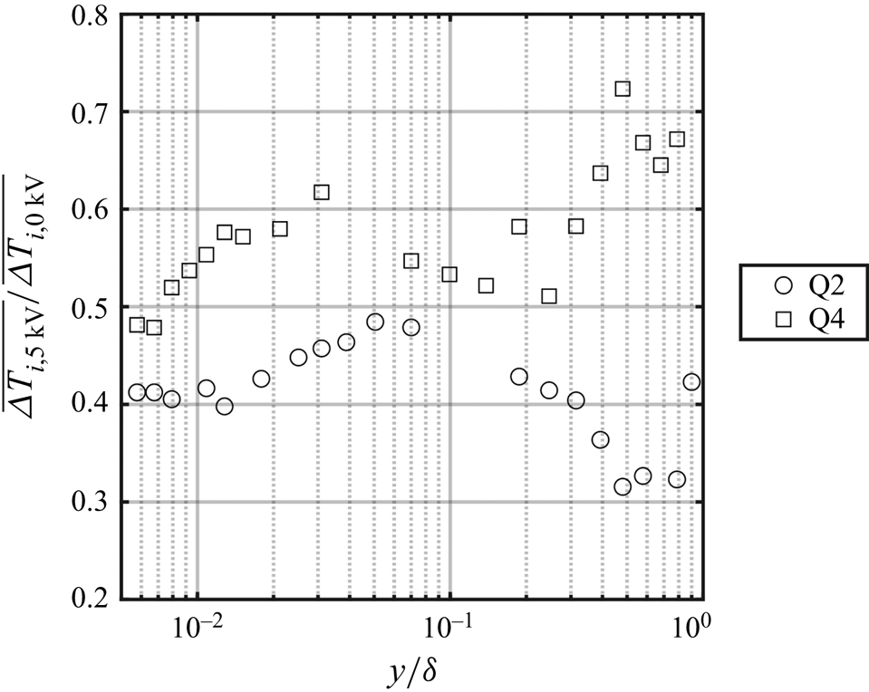
 $\overline {\Delta T_{i}}$, between the baseline and drag-reduced turbulent boundary layers. This is shown across the boundary layer for ejection and sweep events in figures 19 and 20. In the ratios, the event statistic for the drag-reduced boundary layer appears in the numerator so that a value read on the ordinate represents a factor times the event statistic for the baseline boundary layer. Focusing first on the ratio of time between events,
 $\overline {T_{i, 5\ \textrm {kV}}}/\overline {T_{i,0\ \textrm {kV}}}$, figure 19 clearly shows that energetic Q2 and Q4 events are much less frequent in the drag-reduced boundary layer. For example, in the logarithmic region at
 $y/\delta \approx 0.12$ (
 $y^{+}=200$), the interval between successive Q2 events is increased by a factor of 10. For Q4 events at the same location, the interval is increased by a factor of 12. Closer to the wall, the interval between Q2 events is increased by factors of 4 and 5 at
 $y^{+}=15$ and
 $y^{+}=30$, respectively. For Q4 events, the interval increases by factors of 7 and 9 at
 $y^{+}=15$ and
 $y^{+}=30$, respectively.
Comparison of the period of events between baseline and drag-reduced boundary layers for a hyperbolic hole size of  $\alpha = 4$.

Comparison of the duration of events between baseline and drag-reduced boundary layers for a hyperbolic hole size of  $\alpha = 4$.

The effect of the drag reduction on the duration of energetic Q2 and Q4 events is presented in figure 20. With both, the event duration was reduced throughout the boundary layer. Near the wall at  $y^{+}=15$ and
 $y^{+}=30$, the duration of Q2 events are reduced by approximately 58 %. Similarly, the duration of Q4 events was respectively reduced by 45 % and 42 % at
 $y^{+}=15$ and
 $y^{+}=30$. Thus the duration of Reynolds stress producing events in the drag-reduced boundary layer was approximately half of that compared to the baseline boundary layer. Taken together, figures 19 and 20 show that not only was the frequency of Q2 and Q4 events dramatically reduced, but those events that still occur were considerably shorter in duration in the drag-reduced boundary layer. Since these events have been shown to contribute a large portion of the [
 $u^\prime v^\prime$]-Reynolds stress (Corino & Brodkey Reference Corino and Brodkey1969), their reduced duration and increased time between occurrences should affect turbulence production. Furthermore, it is well known that Q2 and Q4 motions will give rise to local shear layers in the boundary layer (so-called uniform momentum zones de Silva, Hutchins & Marusic Reference de Silva, Hutchins and Marusic2016) and can be associated with local turbulence production. This is investigated in the following results.
To investigate the effect of the drag reduction on the boundary layer turbulence production, attention is focused on the production term in the transport equation for the normal stress,  $\overline {u'^{2}}$, namely
 \begin{equation} p ={-}\overline{u^{\prime}v^{\prime}}\frac{\textrm{d}U}{\textrm{d}y}, \end{equation}
which represents the rate of production of  $\overline {u'^{2}}$ from the mean strain rate. This was normalized using outer variables,
 $U_{\infty }$ and
 $\delta$, to obtain the final form,
 \begin{equation} P = p\frac{\delta}{U^{3}_{\infty}} ={-}\overline{u^{\prime}v^{\prime}}\frac{\textrm{d}U}{\textrm{d}\kern0.05em y}\frac{\delta}{U^{3}_{\infty}}. \end{equation}
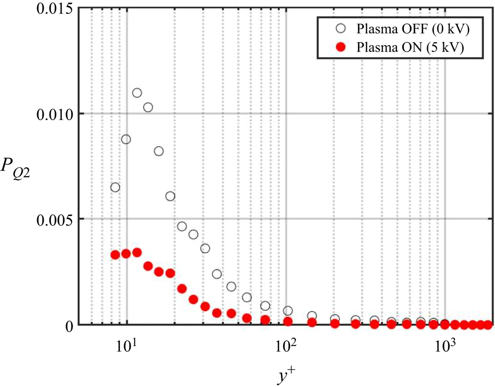
Figure 21 presents a comparison between the baseline and drag-reduced boundary layers of the normalized production,  $P$, determined at different
 $y^{+}$ distances from the wall. These were measured at the same [
 $x,z$] location as the wall-normal profiles shown in previous figures. For the baseline boundary layer, the peak in the turbulence production occurs at approximately
 $y^{+}=12$, in agreement with Klebanoff (Reference Klebanoff1955). When compared to the baseline boundary layer, the turbulence production in the drag-reduced boundary layer decreases everywhere up to
 $y^{+}\approx 400$. The decrease in turbulent production is particularly pronounced near
 $y^{+}=15$, where reductions of approximately 50 % are indicated.
Comparison between baseline and drag-reduced turbulent boundary layers of turbulence production term scaled by outer variables  $U_{\infty }$ and
 $\delta$.

The production results shown in figure 21 included all levels of [ $u^\prime v^\prime$]-Reynolds stress. Using the [
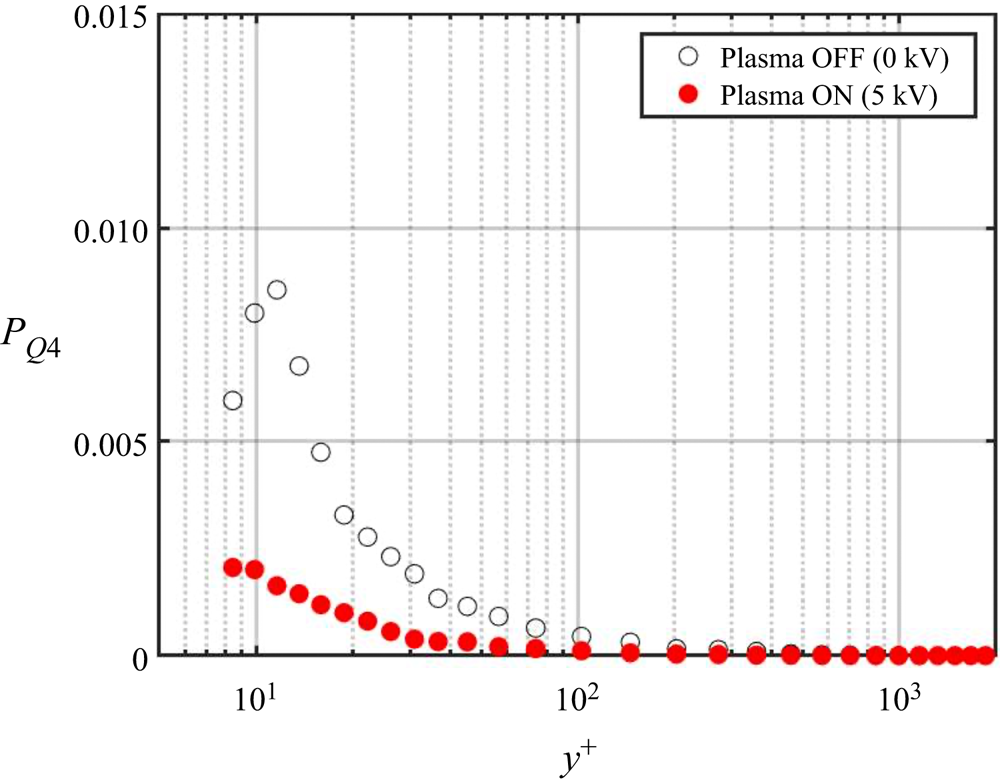
 $u^\prime v^\prime$]-quadrant approach, it is possible to distinguish the contributions to the production of the ejection (Q2) and sweep (Q4) events. This was investigated using a lower threshold value of
 $\alpha =2$, which based on figure 16 still predominately involves only Q2 and Q4 events. The results are shown in figures 22 and 23 for ejection (Q2) and sweep (Q4) events, respectively. As with the production for the baseline boundary layer that included all levels of [
 $u^\prime v^\prime$]-Reynolds stress, the peak in turbulence production for both ejection and sweep events occurs at
 $y^{+}=12$. Also consistent with the previous results is a significant reduction in the turbulence production associated with these events in the drag-reduced boundary layer. For example near
 $y^{+}=15$, production associated with Q2 events was reduced by 71 %, and that associated with Q4 events was reduced by 79 %. The following section explores changes in the near-wall coherent structures that occurred in the drag-reduced boundary layer, and are generally associated with the previous ejection–sweep dynamics.
Comparison between baseline and drag-reduced turbulent boundary layers of turbulence production associated with ejection (Q2) events based on  $\alpha =2$ threshold.

Comparison between baseline and drag-reduced turbulent boundary layers of turbulence production associated with sweep (Q4) events based on  $\alpha =2$ threshold.

3.3. Conditional flow field reconstruction
In order to further investigate the effect of the flow control on the coherent structures in the near-wall region of the boundary layer, conditional-averaged reconstructions of the flow field were performed. For this, the X hot-wire probe at the fixed [ $x,z$] location was lowered to
 $y^{+}=15$. Recall that the fixed probe was located at
 $x^{+}=115$ downstream of the plasma actuator array, where the results in figure 11 had indicated conditions were representative of those over the plasma array. The fixed probe provided the [
 $u,v$] time series used to define ‘events’ on which the conditional averages were based. The other X hot-wire probe was located at the same
 $x$ location as the fixed probe, and moved in the [
 $y,z$] direction with the same range as used to compile results in figure 5. The time series from both X hot-wire probes were sampled simultaneously.
The method for defining an ‘event’ utilized the ‘variable-interval time-averaged’ (VITA) technique that was pioneered by Blackwelder & Kaplan (Reference Blackwelder and Kaplan1976). This utilized the  $u$ velocity time series and applied a discriminator,
 $D$, such that
 \begin{equation} D(t)
= \begin{cases} 1 & \text{if}\
\widehat{\textrm{var}} > ku^{\prime 2}_{rms},\\ 0 &
\text{Otherwise}, \end{cases}
\end{equation}
where
 \begin{equation} \widehat{\textrm{var}}(x_i,t,T)=\widehat{u^{\prime 2}}(x_i,t,T) - [\widehat{u^\prime}(x_i,t,T)]^2 \end{equation}
is the localized variance of streamwise velocity fluctuations over the interval  $T$ at a spatial location,
 $x_i$. With this discriminator, Blackwelder & Kaplan (Reference Blackwelder and Kaplan1976) recommended that
 $k=1.2$, and that
 $Tu_{\tau }^2/\nu = 10$. Furthermore, they applied the detection at
 $y^{+}=15$ in the boundary layer, where the turbulence intensity was a maximum. The conditionally averaged velocity field that results from VITA detection is thought to embody the initial ‘ejection’ of low momentum fluid from the wall that is followed by a faster moving ‘sweep’ of fluid that approaches from outside the wall region (Blackwelder & Kaplan Reference Blackwelder and Kaplan1976).
Once a reference time for each VITA event was determined by the detection function,  $D(t)$, the characteristics of the flow field in time and space were constructed based on a conditional average defined as
 \begin{equation} \langle Q(y_i,z_i,T)\rangle_{y^{+}=15} = \frac{1}{N}\sum_j^N Q(y_i,z_i,t_j+T), \end{equation}
where  $Q$ is the estimated quantity which is a function of the independent variables [
 $y_i,z_i$] that denote the position in space of the moving probe where the sampling occurred, and the subscript
 $y^{+}=15$ denotes the wall-normal position of the fixed probe where the detection occurred. The quantities
 $t_j$ are those points in the time series when a detection occurred. Since
 $D(t)$ was equal to unity only during very short time intervals, the times
 $t$, were taken to be midway between the beginning and end of the period during which
 $D(t)\neq 0$. A positive or negative time delay
 $T$ with a range of
 $-4 \leq T^* \leq 4$, was used to determine the temporal behaviour of
 $Q$ before or after a detection occurred.
 $N$ is the total number of samples added in the ensemble average.
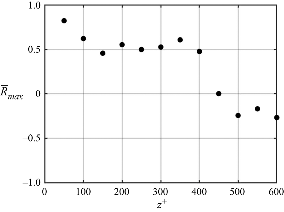
As a first step, it was important to determine the spanwise extent over which detected events were correlated. This is presented for the baseline boundary layer in figure 24, which documents the correlation coefficient,  $[\bar {R}(z^{+},\tau )]_{max}$, of events detected by the fixed probe to that detected by the moving probe. It is defined as the covariance normalized by the product of the standard deviations, or
 $R=\sigma [u(z^{+}_{ref},t)u(z^{+},t+\tau )]/(\sigma [u(z^{+}_{ref})]\sigma [u(z^{+})])$.
 $R$ ranges from
 $\pm 1$. Both probes were located at
 $y^{+}=15$. The spanwise range of the moving probe was
 $50 \leq z^{+} \leq 600$. The results indicate a reasonable spatial correlation, prior to a sharp drop off that extended to
 $z^{+}=400$. This was then taken as the spanwise limit over which flow reconstructions were considered valid. Based on an average
 $z^{+}=100$ spacing between wall streak structures (Kline et al. Reference Kline, Reynolds, Schraub and Runstadler1967), the correlated region encompasses four streak structures.
Spanwise correlation coefficient,  $[\bar {R}(z^{+},\tau )]_{max}$, between the fixed probe at
 $y^+=15$ and
 $z^{+}=0$, and moving probe at
 $y^{+}=15$ and
 $50 \leq z^{+} \leq 600$.

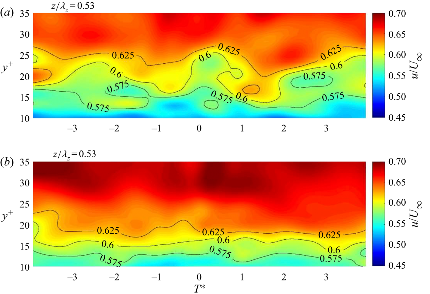
Figure 25 shows the conditionally averaged  $u^\prime$ turbulence levels in the [
 $y^{+},T^*$] plane at
 $z^{+}=50$ for the baseline and drag-reduced boundary layers. The
 $u'/U_{\infty }$ levels are shown as constant level colour contours. These are further denoted by the solid-line curves on which the
 $u'/U_{\infty }$ levels are listed. These focus on the near-wall region with
 $y^{+}\leq 35$.
 $T^*=0$ corresponds to the time of the VITA detection. In the orientation with negative
 $T^*$ to the left of
 $T^*=0$, the equivalent flow direction is from left to right.
Constant level contours of  $\langle u^\prime /U_{\infty }(y_i^{+},z_{50}^{+},T^*)\rangle _{y^{+}=15}$ for the baseline boundary layer (a) and drag-reduced boundary layer (b).

The contours for the baseline boundary layer indicate quasi-periodic ‘bulges’ that extend out to approximately  $y^{+}=30$. The VITA discriminator is a sharp gradient in the
 $u^\prime (t)$. This is apparent at
 $T^*=0$ for the baseline boundary layer. The other ‘bulges’ with sharp gradients are not necessarily related to the detected event at
 $T^*=0$, but were statistically present in the ensemble at the time of the detection. The average time between ‘bulges is approximately
 $\Delta T^*=3$. This is the same order of an average
 $U_{\infty }T/\delta =5$ suggested by Laufer & Narayanan (Reference Laufer and Narayanan1971).
In contrast to the baseline boundary layer, the wall-normal extent of the same  $u'/U_{\infty }$ magnitudes is significantly less for the drag-reduced boundary layer. This includes the extent and duration of the ‘bulges’, which are also observed to occur less frequently over the same time period. This is consistent with the previous [
 $u^\prime v^\prime$]-quadrant splitting results that documented a weakening of the ejection–sweep events in the drag-reduced boundary layer.
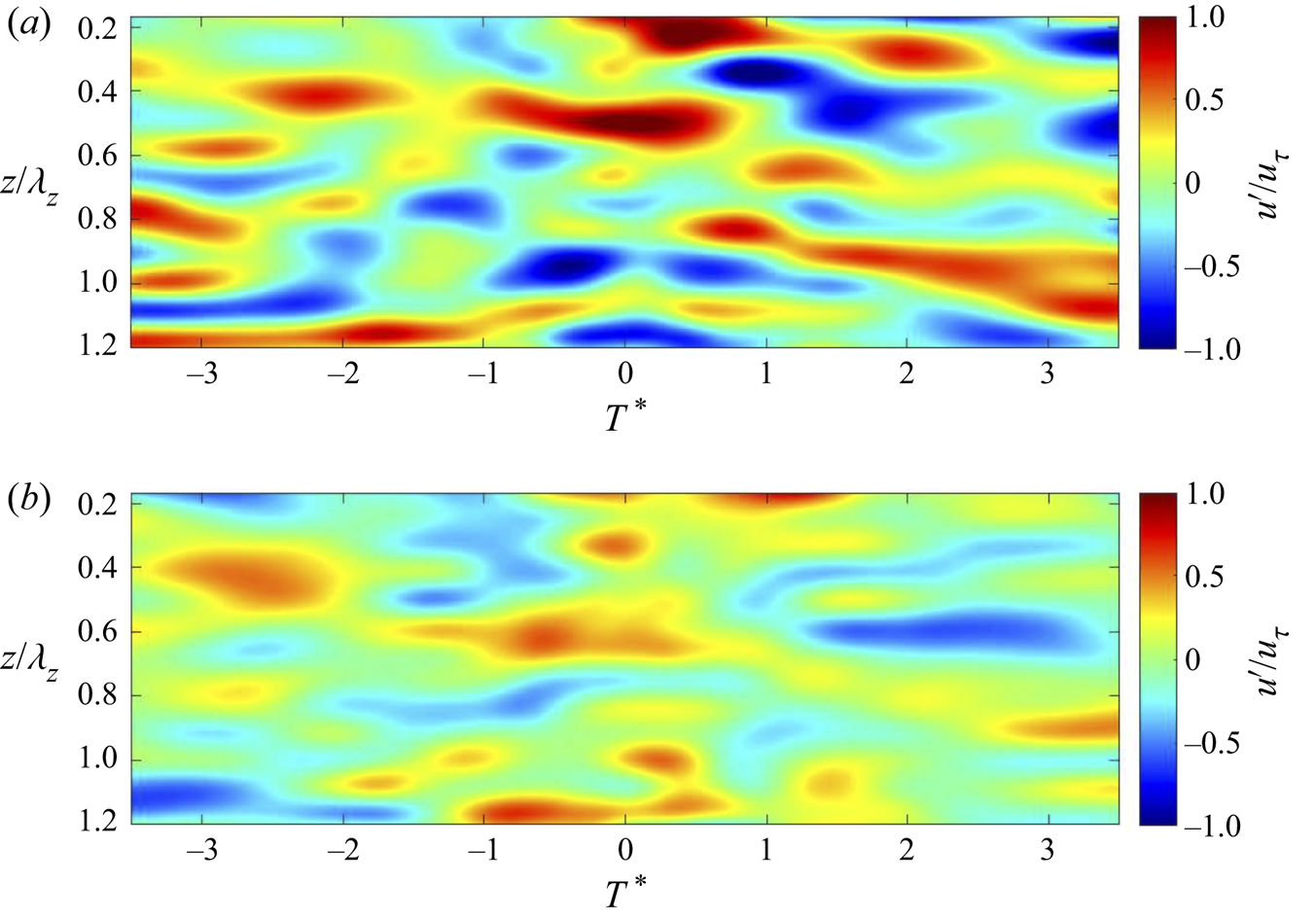
The underlying assumption for the flow control was to reduce the spanwise mean flow distortion that flanks the wall streak structure. To investigate this effect, the conditionally averaged  $u^\prime /u_{\tau }$ levels in the [
 $z^{+},T^*$] plane are presented in figure 26 at a
 $y^{+}=30$ for the baseline and drag-reduced boundary layers. As before, the levels are shown as constant level colour contours. For this, the
 $z^{+}$ distance has been normalized by the
 $\lambda ^{+}_z=300$ spacing between exposed electrodes of the plasma actuator array. For reference, the
 $z^+=100$ average wall streak structure spacing (Kline et al. Reference Kline, Reynolds, Schraub and Runstadler1967) corresponds to
 $z^{+}/\lambda ^{+}_z = 0.3$.
Constant level contours of  $\langle u^\prime /u_{\tau }(y_{30}^{+},z^{+}/\lambda ^{+}_z,T^*)\rangle _{y^{+}=15}$ for the baseline boundary layer (a) and drag-reduced boundary layer (b).

The contours for the baseline boundary layer indicate features that are elongated in the streamwise direction. As before, the equivalent flow direction is from left to right. The average spanwise spacing of these features is fairly close to the  $z^{+}/\lambda ^{+}_z = 0.3$ that would correspond to the average wall streak structure spacing (Kline et al. Reference Kline, Reynolds, Schraub and Runstadler1967). In a locally convected frame, the mean
 $T^*$ extent of the features shown for the baseline case correspond to a streamwise length of
 $x^{+}\sim O(1000)$. In contrast to the baseline boundary layer, the
 $u^\prime /u_{\tau }$ magnitudes are again significantly less for the drag-reduced boundary layer. This has resulted in an increase in the region of low
 $u^\prime$ levels, that indicates an increase in the streamwise and spanwise spacing between the elongated features. The increased spanwise spacing reflects the decrease in
 $u_{\tau }$ so that the physical spacing
 $z u_{\tau }/\nu \simeq 100$ is maintained.
The previous figure presented a view at one height in the boundary layer. In order to provide a more complete depiction of the effect of the drag reduction, a 3-D view based on vorticity was constructed from the conditionally averaged flow field. As a result of only measuring the  $u$ and
 $v$ velocity components, only the
 $z$-component of vorticity was calculated, namely
 $\omega _z= \partial v/\partial x - \partial u/\partial y$. In determining
 $\partial v/\partial x$, a frozen flow assumption was assumed with a convection velocity of
 $0.6U_{\infty }$ which corresponds to the local mean velocity at
 $y^{+}=30$ in the baseline boundary layer. Isometric views of a vorticity isosurface of
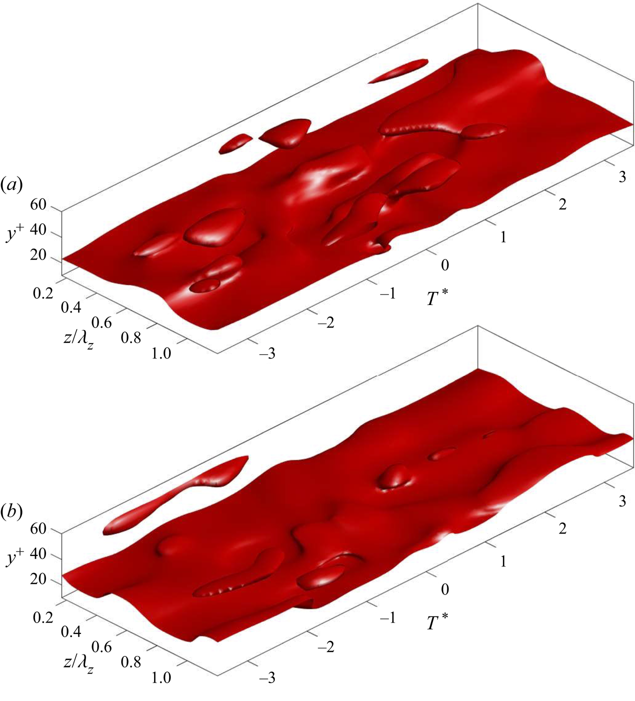
 $|\omega ^{+}_z|=0.1$ are shown for the baseline and drag-reduced boundary layers in figure 27. These support the previous results with a noticeably reduced extent of 3-D features in the wall layer, along with a general smoothing of the vorticity isosurface in the drag-reduced boundary layer.
Vorticity isosurface of  $\langle |\omega ^{+}_z|(y^{+},z^{+}/\lambda ^{+}_z,T^*)\rangle _{y^{+}=15}=0.1$ for the baseline boundary layer (a) and drag-reduced boundary layer (b).

The  $\lambda _{2}$ criterion (Jeong & Hussain Reference Jeong and Hussain1995) was then used to further quantify the difference in the vorticity dynamics between the baseline and drag-reduced boundary layers. As outlined by Jeong & Hussain (Reference Jeong and Hussain1995),
 $\lambda _{2}$ is the second invariant (eigenvalue) of the local pressure Hessian that is based on the local minimum of pressure that corresponds to a vortex centre. The method required several steps to compute the second eigenvalue for each point in the event conditioned velocity field. First, the gradient velocity tensor,
 $P = \nabla u$, was computed for each [
 $y^{+},z^{+},T^*$] point in the velocity field;
 $P$ was then decomposed into symmetric and anti-symmetric parts defined as
 $S = \frac {1}{2}(P + P^{T})$ and
 $A = \frac {1}{2}(P - P^{T})$ from which the eigenvalues of
 $S^{2} + A^{2}$ were computed. In our case,
 $\lambda _2$ was calculated in 2-D [
 $y^{+},T^*$] planes for different
 $z^{+}/\lambda ^{+}_z$ locations, and then pieced together to form a 3-D representation. For the 2-D flow field slices, only two eigenvalues were needed. These were ordered as
 $\lambda _{1} \ge \lambda _{2}$, where a vortex was defined as connecting regions of
 $\lambda _{2} < 0$ (Jeong & Hussain Reference Jeong and Hussain1995). Again, because only
 $u$ and
 $v$ velocity components were measured, only
 $\omega _z$ could be calculated. We acknowledge that this approach is not as comprehensive as computing the 3-D
 $\lambda _2$ structures, and that they represent the invariant of only the
 $\omega _z$ component.
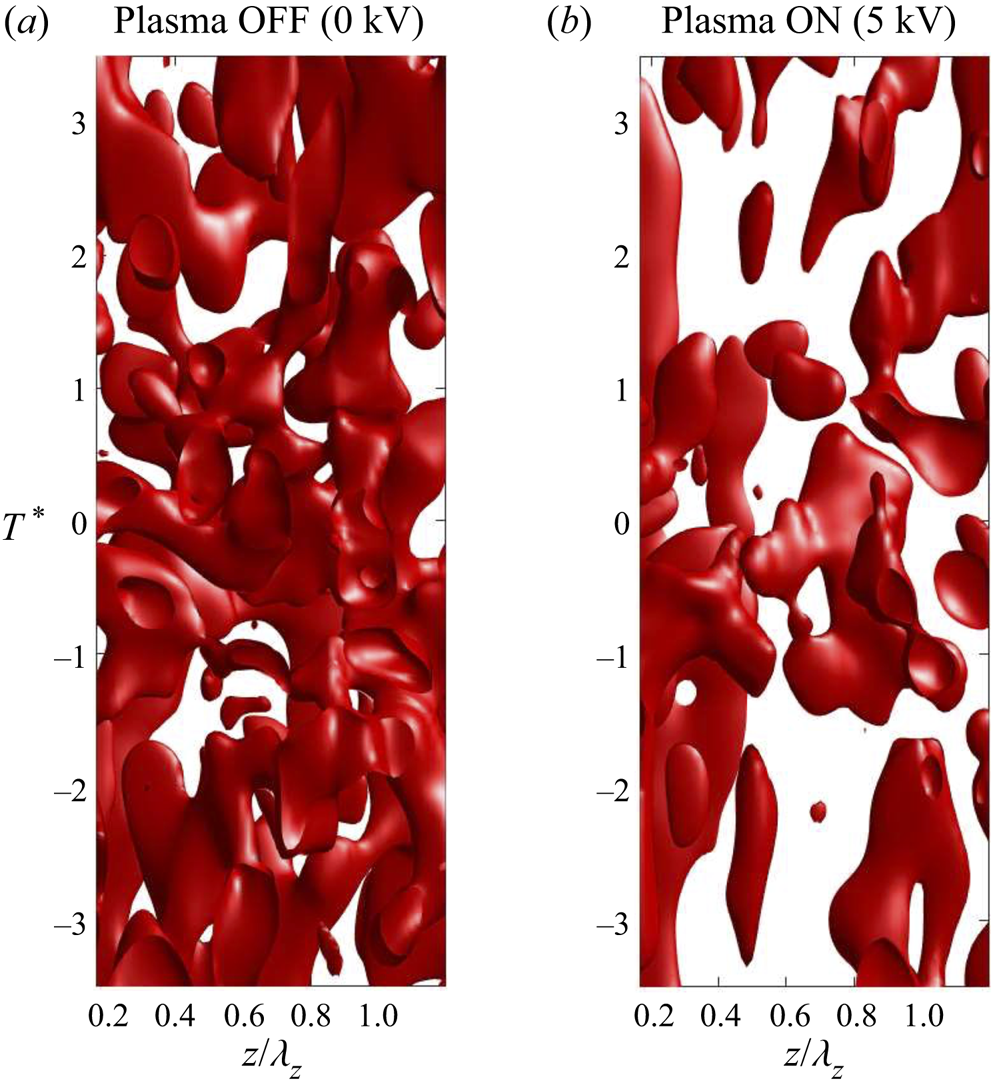
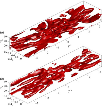
While the  $\lambda _2$ criterion as applied may not form a complete view of the vorticity field, it does reinforce the previous observed differences in the near-wall structure between the baseline and drag-reduced boundary layers. This is presented in figures 28 and 29. These present isosurfaces of
 $\lambda _2=-1.25$. These views illustrate both an increase in the spacing of the
 $\lambda _2$ structures, as well as a lowering of their wall-normal extent in the drag-reduced boundary layer, compared to the baseline boundary layer. These observations are consistent with the underlying premise that the flow control that produced the viscous drag reduction, is simultaneously suppressing the cycle of low-speed fluid lift-up associated with turbulence fluctuations and production, in the wall layer.
Vorticity isosurface -p plasma OFF (0 kV). Top–down views of  $\langle \lambda _2(y_i^{+},z_i^{+},T^*)\rangle _{y^{+}=15}=-1.25$ isosurface for baseline boundary layer (a) and drag-reduced boundary layer (b).

Isometric views of  $\langle \lambda _2(y_i^{+},z_i^{+},T^*)\rangle _{y^{+}=15}=-1.25$ isosurface for baseline boundary layer (a) and drag-reduced boundary layer (b).

4. Conclusions
Experiments were performed using an active flow control approach that has shown the ability to significantly reduce the viscous drag in turbulent boundary layers. The flow control involved generating a steady spanwise velocity component of the order of  $u_{\tau }$, within the sublayer using an array of pulsed-DC plasma actuators similarly employed and characterized by Thomas et al. (Reference Thomas, Corke, Duong, Midya and Yates2019), Duong (Reference Duong2019) and Duong et al. (Reference Duong, Midya, Corke, Hussain and Thomas2019). The intent was to reduce the wall-normal vorticity component,
 $\omega _y$, that is associated with the mean flow distortion caused by quasi-steady streamwise vorticity associated with the wall streak structure first observed by Kline et al. (Reference Kline, Reynolds, Schraub and Runstadler1967). The significance of the
 $\omega _y$ comes from Schoppa & Hussain (Reference Schoppa and Hussain1998) who proposed a mechanism for the self-sustained generation of new vorticity in the buffer layer, and based on Kim (Reference Kim2011), is linked to skin friction drag.
The results compared the characteristics of a baseline turbulent boundary layer to those in which the viscous drag was reduced by 68 %. This involved measurements of  $u$ and
 $v$ velocity components in 3-D space using a pair of dual (X) hot-wire probes. The turbulence intensity profiles documented a significant decrease in the
 $u$ and
 $v$ fluctuations that were largest in the near-wall region, but extended throughout the boundary layer. Using this characteristic decrease as an indicator of the degree of drag reduction, an approximate
 $x^+ = 300$ development length was needed to reach the maximum drag-reduction level over the actuator array. This corresponded to the first 21 % of the streamwise length of the actuator array. The reduced turbulence levels (correlating with drag reduction) persisted to the most downstream measurement location, which was
 $x^+ = 440$ beyond the downstream actuator array. It remains an open and important question of how much further downstream it persisted.
When the reduction in the turbulence intensity levels in the drag-reduced boundary were scaled by  $u_{\tau }$, it was found that the
 $v^\prime$ turbulence intensity was affected more, with an average reduction across the log layer of 22 %. The average reduction for the
 $u^\prime$ turbulence intensity scaled by
 $u_{\tau }$, was 16 %.
The  $[u^\prime v^\prime ]$ quadrant method was used to quantify the contributions of ejection (Q2) and sweep (Q4) events on the [
 $\overline {u^\prime v^\prime }$]-Reynolds stress production in the drag-reduced boundary layer. Analysis showed large increases in the time between both Q2 and Q4 events, as well as a shortening of their durations in the drag-reduced boundary layers. The net result was a large reduction in the dynamical significance of these events that was manifest in the turbulent production, particularly in the near-wall region. Overall, the largest effect was on ejection (Q2) events, which is consistent with a suppression of low-speed fluid lift-up that was correlated with the drag reduction.
When compared to the baseline boundary layer, the turbulence production in the drag-reduced boundary layer decreased everywhere up to  $y^{+} = 400$. The decrease in turbulent production was particularly pronounced at
 $y^{+} = 15$, where the maximum production occurred in the baseline boundary layer. No peak at
 $y^{+} = 15$ was evident in the drag-reduced boundary layer. Also with the drag reduction, the turbulence production through ejection (Q2) and sweep (Q4) events was respectively reduced by 71 % and 79 %.
Conditional averages were used to reconstruct the 3-D coherent motions associated with an event defined by the VITA technique that utilized a peak in the localized variance in streamwise velocity fluctuations as a discriminator. These events were found to be correlated in the spanwise direction out to  $z^{+}=400$. Conditional reconstruction of the
 $u^\prime /U_{\infty }$ in the [
 $y^{+},T^*]$-plane for the baseline boundary layer indicated quasi-periodic bulges in constant level contours that extended out to
 $y^+=30$. The average time between bulges was of the order of
 $T U_{\infty }/\delta =5$. In contrast, in the drag-reduced boundary layer, the wall-normal extent of the same magnitude contours was significantly reduced, as well as the time between bulges significantly extended.
Conditional reconstruction of  $u^\prime /u_{\tau }$ in the
 $[z^{+},T^*]$-plane indicated features that were elongated in the streamwise direction with an average spanwise spacing of
 $z^{+}=100$. The average temporal extent of the features was
 $T U_{\infty }/\delta \approx 1.1$ which, in a locally advected frame, corresponds to a streamwise spatial extent of
 $x^{+}\approx 950$. The scale of these features is consistent with streamwise vortices in the buffer layer that are associated with the wall streak structure. In contrast to the baseline boundary layer, the
 $u^\prime /u_{\tau }$ magnitudes were significantly less for the drag-reduced boundary layer. This resulted in an increase in the region of low
 $u^\prime$ levels that gave the appearance of increased spanwise and streamwise spacing between the elongated features in the drag-reduced boundary layer.
Conditional 3-D reconstructions of the  $\omega _z$ vorticity provided a similar view with a noticeable reduction in the magnitude and streamwise extent of elongated features in the drag-reduced boundary layer. This was further reinforced by a comparison between the baseline and drag-reduced boundary layers of 3-D reconstructions of
 $\lambda _2$ isosurfaces.
The flow control approach was motivated in part, by simulations by Schoppa & Hussain (Reference Schoppa and Hussain1998) that observed that spanwise blowing in the wall layer of a turbulent channel flow resulted in a 50 % reduction in the viscous drag. They associated this effect with a lessening of the local spanwise mean flow distortion in the region flanking the low-speed wall streak structure. Later, Schoppa & Hussain (Reference Schoppa and Hussain2002) linked this result to control of ‘streak transient growth’ in which the local  $\omega _y$ is a critical parameter. The premise was that this control would actively intervene with an autonomous cycle involving lift-up and break-up of coherent streamwise vorticity that is associated with the low-speed wall streak structure. The present experimental results are fully consistent with this premise.
Acknowledgements
The information presented in this report is based upon work through Phase II SBIR with Innovative Technology Applications under NASA Contract NNX16CL27C.
Declaration of interests
The authors report no conflict of interest.
Data availability statement
The data that support the findings of this study are openly available in Duong (Reference Duong2019).