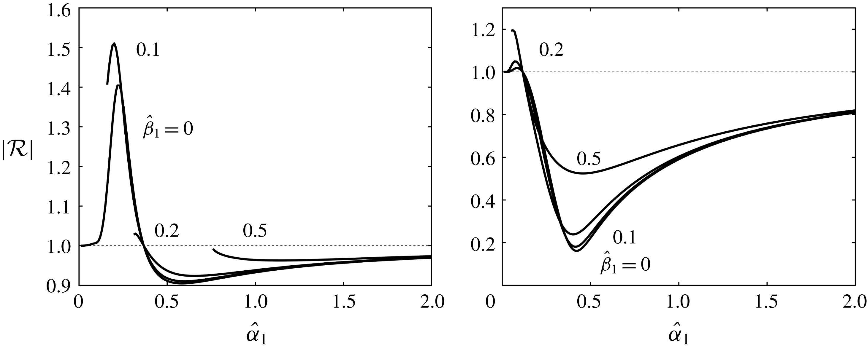
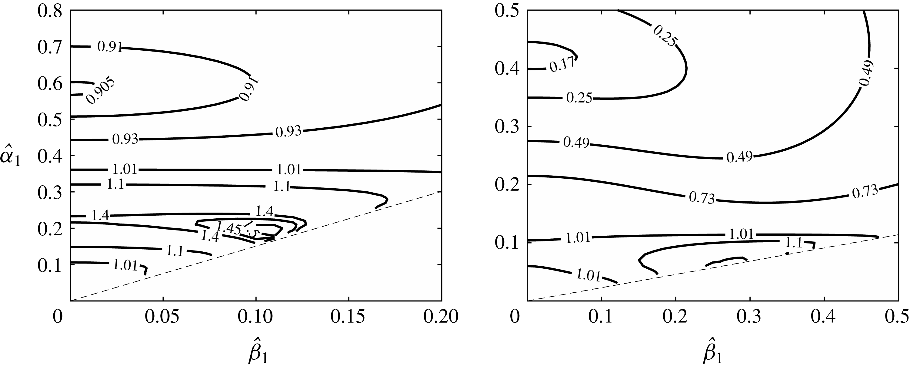
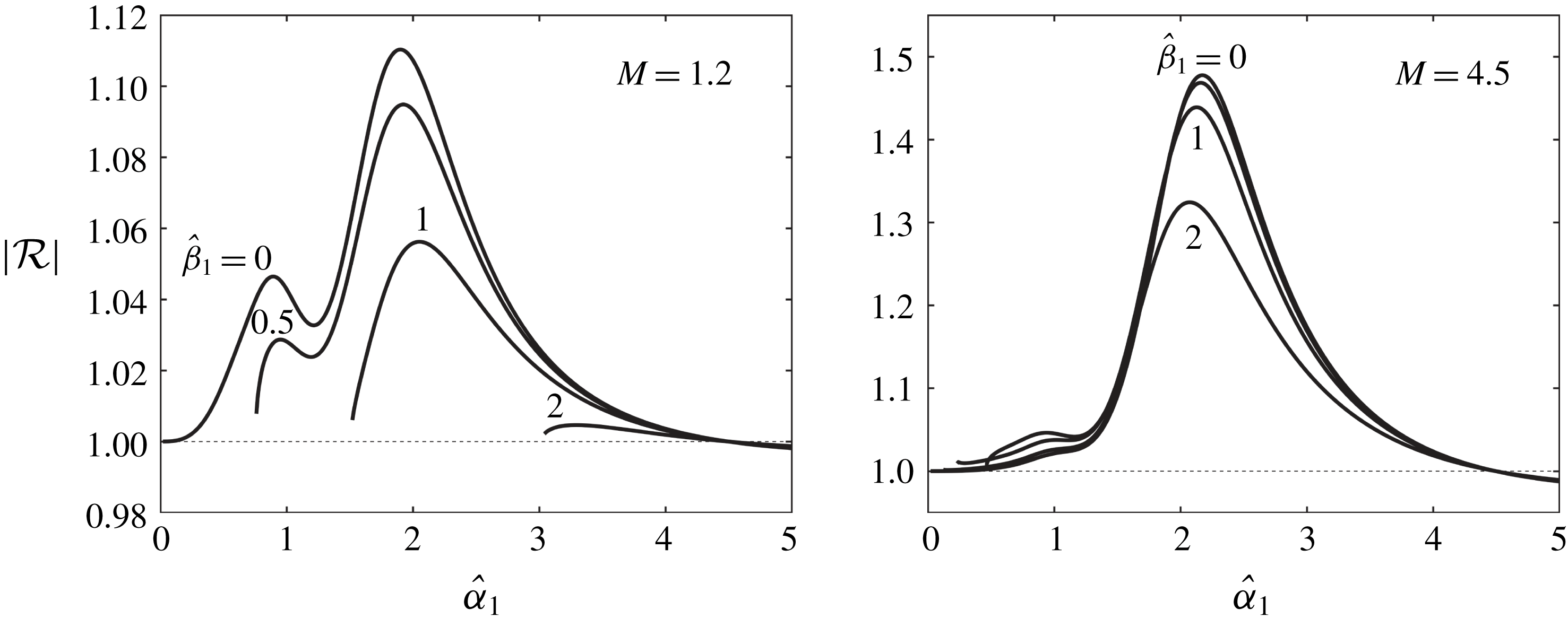
1 Introduction
Laminar–turbulent transition of boundary layers represents an extraordinarily complicated process, which is, at present, not fully understood. It has numerous technological applications, e.g. being important for the prediction and reduction of drag and noise. In the supersonic regime, boundary-layer transition plays a crucial role in the correct characterization of the flow and thermal fields around high-speed vehicles (Fedorov Reference Fedorov2011). In the presence of low-level free-stream turbulence, transition occurs via the so-called natural route, which involves a sequence of stages (Morkovin, Reshotko & Herbert Reference Morkovin, Reshotko and Herbert1994) starting with receptivity, followed by linear instability, nonlinear growth and breakdown to turbulence (Morkovin Reference Morkovin1969; Reshotko Reference Reshotko1976).
Boundary-layer receptivity refers to the process in which external perturbations (e.g. oncoming sound waves, free-stream turbulence and entropy and localized or distributed roughness) excite instability modes. These intrinsic instabilities may amplify to attain amplitudes far above those of the external disturbances, eventually leading the boundary layer to turbulence. Instability modes that may arise depend on the Mach number. In the subsonic regime, they are Tollmien–Schlichting (T–S) waves, which have a viscous origin. In the super- and hyper-sonic regimes, there exist multiple families of modes (Mack Reference Mack1984) including the so-called first Mack modes, which are continuation of T–S modes into the compressible regime, and the second Mack modes, which are essentially inviscid.
Mathematically, the problem of receptivity is different from that of stability. The latter seeks normal modes, which gives rise to an eigenvalue problem. In receptivity theory, because of external forcing, an inhomogeneous boundary-value problem arises. A general unsteady disturbance in a uniform compressible flow can, to leading order, be decomposed into three independent components: acoustic, vorticity and entropy modes (Kovasznay Reference Kovasznay1953). The first is a pressure fluctuation, which propagates through the fluid with the speed of sound. The other two represent, respectively, vorticity and temperature perturbations being convected at the free-stream velocity, and they have been used to model free-stream turbulence in many applications. Usually, none of the external disturbances alone can excite T–S waves because its wavelength would differ from those of the latter if its frequency is chosen to be the same. A crucial task of receptivity study is to identify the scale conversion or matching mechanism, by which the length and time scales of external disturbances are adjusted to match those of the instability, or the external disturbances produce a forcing with the length and time scales matching with those of the instability. The main goal of studying receptivity is to determine the amplitudes of the generated instability waves and, linked to the former, to identify which types of external disturbances can trigger the instability more effectively.
Shapiro (Reference Shapiro1977) and Kachanov, Kozlov & Levchenko (Reference Kachanov, Kozlov and Levchenko1979) were among the earliest to study experimentally the generation of T–S waves by free-stream acoustical and vortical disturbances, respectively. Although the leading edge region was found to be important for excitation, the precise mechanisms had remained unknown until several theoretical discoveries on boundary-layer receptivity were made in the 1980s; for a detailed review, see, for example, Goldstein & Hultgren (Reference Goldstein and Hultgren1989). The triple-deck theory, which is based on high-Reynolds-number asymptotic approximations, has played an important role; this is not surprising since this formalism simplifies the mathematical description of the instability and specifies precisely the time and length scales of the instability modes (Lin Reference Lin1945; Smith Reference Smith1979), which is crucial for studying receptivity. Using this approach, Terent’ev (Reference Terent’ev1981) first analysed the generation of T–S modes by a short vibrating section of a flat plate. The vibrating section generates a T–S wave effectively when its frequency and length are comparable with the characteristic frequency and wavelength of the T–S wave. Goldstein (Reference Goldstein1983) showed that a long-wavelength sound wave interacts with the strongly non-parallel mean flow near the leading edge, first to excite an asymptotic eigensolution called Lam–Rott mode. As its wavelength shortens due to the increase of the boundary-layer thickness, the Lam–Rott eigensolution finally evolves into a lower-branch T–S mode. This solution however undergoes severe decay before reaching the neutral stability point, rendering the mechanism fairly weak. A more efficient mechanism was proposed independently by Ruban (Reference Ruban1984) and Goldstein (Reference Goldstein1985), in which a weak sound wave interacts with a roughness-induced perturbation to excite a T–S wave downstream. They pointed out that for T–S waves to be generated by acoustic disturbances, a resonance condition must hold, which means that the frequency of the oncoming sound must be chosen to be that of the T–S waves. Since this choice would make the wavelength much larger than that of T–S waves, it is crucial to introduce a length scale comparable with the wavelength of the T–S waves. This is achieved by including a suitable wall roughness, which causes a stationary disturbance in the boundary layer; an acoustic wave interacts with it to produce an unsteady forcing, whose length scale and frequency match those of the T–S waves. Ruban, Bernots & Kravtsova (Reference Ruban, Bernots and Kravtsova2016) extended this theory to transonic boundary layers. De Tullio & Ruban (Reference De Tullio and Ruban2015) performed direct numerical simulations (DNS) of the receptivity of subsonic compressible boundary layers to roughness–sound interaction. A comparison with the results of the asymptotic (triple-deck) theory showed that the latter hold down to moderate Reynolds numbers
 $R=O(10^{5})$
, showing a good agreement for Mach number
 $M=0.8$
, and excellent agreement for
 $M=0.2$
.
Duck, Ruban & Zhikharev (Reference Duck, Ruban and Zhikharev1996) considered the receptivity to free-stream vortical disturbances interacting with a localized roughness element on a flat plate. They demonstrate that although this type of disturbance does not penetrate into the boundary layer, it can interact with the roughness-induced perturbation at the outer edge of the boundary layer, thereby producing a forcing to generate a T–S mode. Dietz (Reference Dietz1999) conducted a detailed experimental study of the receptivity to vortical disturbances which were introduced in a controlled manner. A comprehensive set of data was acquired. Prompted by these data, Wu (Reference Wu2001a ) extended the analysis of Duck et al. (Reference Duck, Ruban and Zhikharev1996) to second order and to vortical disturbances with an arbitrary transverse distribution; the latter made a quantitative comparison with experiment possible. A good agreement was found between the second-order theory and the measurements.
A finite-Reynolds-number approach to receptivity was formulated by Zhigulev & Fedorov (Reference Zhigulev and Fedorov1987), Choudhari & Streett (Reference Choudhari and Streett1992) and Crouch (Reference Crouch1992). This method retains the essence of the Goldstein–Ruban theory, but uses inhomogeneous Orr–Sommerfeld (O–S) equations instead of the triple-deck equations to compute the mean-flow distortion as well as the resultant T–S waves. The accuracy of the predictions was confirmed by comparisons with experiments. Of course, this approach is applicable to roughness with a sufficiently small height. For roughness elements with large enough heights that the mean-flow distortion becomes nonlinear, the O–S equation fails to describe both the mean-flow distortion and the scattering. The triple-deck or interactive boundary-layer formalisms need to be used instead (Goldstein, Leib & Cowley Reference Goldstein, Leib and Cowley1987; Bodonyi et al. Reference Bodonyi, Welch, Duck and Tadjfar1989; Nayfeh & Ashour Reference Nayfeh and Ashour1994).
Receptivity due to the interaction of sound waves or vortical disturbances with a distributed roughness has also been addressed in the literature. The interaction can produce an unsteady forcing that has the frequency and wavenumber of a neutral mode. A theoretical study was made by Crouch (Reference Crouch1992, Reference Crouch1994), using a finite-Reynolds-number (O–S equation) approach. However, the analysis did not consider the resonance region in the vicinity of the neutral curve, where the forcing resonates with the neutral T–S mode. Wu (Reference Wu2001b
) presented a (second-order) asymptotic theory based on the triple-deck formalism. By analysing the resonance region, which is of crucial importance for determining correctly the initial amplitude of the excited T–S wave, he showed that the distributed receptivity is much stronger than that for localized roughness, with the coupling coefficient being larger by a factor of
 $O(R^{3/16})$
. The resonance could only be correctly accommodated by accounting for the non-parallel-flow effect.
The receptivity mechanisms highlighted above have also been studied experimentally and by DNS. The reader is referred to King & Breuer (Reference King and Breuer2002), Saric, Reed & Kerschen (Reference Saric, Reed and Kerschen2002) and Würz et al. (Reference Würz, Herr, Wörner, Rist, Wagner and Kachanov2003) for details. In summary, in the subsonic regime, boundary-layer receptivity, especially to acoustical disturbances, is quite well understood and accurately predicted, except for the case of extremely strong sound waves, where nonlinear effects arise and require further investigation (Saric & White Reference Saric and White1998).
Receptivity of supersonic boundary layers is less well understood in comparison with their subsonic counterparts. Mack (Reference Mack1984) and Ma & Zhong (Reference Ma and Zhong2003) documented in great detail various inviscid and viscous instability modes, which were identified primarily by extensive numerical computations solving the Rayleigh and O-S equations. Relevant high-Reynolds-number asymptotic descriptions were given by Smith (Reference Smith1989), Smith & Brown (Reference Smith and Brown1990) and Blackaby, Cowley & Hall (Reference Blackaby, Cowley and Hall1993) among others. Most receptivity mechanisms identified for subsonic boundary layers continue to operate, but with additional physical parameters (e.g. Mach number) and modes on different scalings, their effectiveness may differ significantly, and new mechanisms may be in action. Fedorov & Khokhlov (Reference Fedorov and Khokhlov1991) and Fedorov (Reference Fedorov2003b ) elucidated how the scattering and diffraction of acoustic waves in the leading-edge region generate the so-called slow and fast instability modes, which are the earliest form of instability. Fedorov (Reference Fedorov2003a ) analysed the generation of second Mack modes due to acoustic waves interacting with localized and distributed surface roughness, whereas Fedorov (Reference Fedorov2013) investigated receptivity to small solid particles present in the free stream. Wu (Reference Wu1999) proposed a different mechanism, in which a sound wave and a vortical disturbance with suitable frequencies and wavenumbers interact to generate a forcing in resonance with, and hence generate, a neutral T–S mode. More recently, Qin & Wu (Reference Qin and Wu2016) studied the receptivity of a hypersonic boundary layer past a wedge, where the shock emanating from the apex makes a small angle with respect to the wedge surface, and thus changes the instability substantially (Blackaby et al. Reference Blackaby, Cowley and Hall1993). They showed that each of the three types of free-stream disturbances interacts with the shock to produce a slow acoustic wave downstream which can resonate with a T–S mode.
Experimental studies of supersonic boundary-layer receptivity are extremely difficult, and only a few have been carried out (e.g. Kendall Reference Kendall1975; Maslov et al.
Reference Maslov, Shiplyuk, Sidorenko and Arnal2001; Semionov & Kosinov Reference Semionov and Kosinov2008). DNS therefore stand as a useful tool. Balakumar (Reference Balakumar2003, Reference Balakumar2005) and Ma & Zhong (Reference Ma and Zhong2003, Reference Ma and Zhong2005) performed DNS of the receptivity of the supersonic boundary layer over a flat plate. The leading edge and the shock are taken into account in their computations. The numerical results showed that in the presence of free-stream acoustical, vortical and entropy disturbances, the first and second modes are excited. Qualitatively similar findings have also been revealed for boundary layers over a parabola, blunt plates and cones; the reader is referred to Zhong & Wang (Reference Zhong and Wang2012) for details. However, the precise excitation mechanisms and processes are yet to be fully clarified. It appeared that the free-stream disturbances interact first with the shock, generating acoustic waves downstream, which then excite slow and fast instability modes through the mechanism of Fedorov & Khokhlov (Reference Fedorov and Khokhlov1991). The slow mode evolves into a first Mack mode. Further downstream, the first mode and the fast mode may be converted to a second mode at the so-called synchronization point (Fedorov & Khokhlov Reference Fedorov and Khokhlov2001). This interpretation is applicable to instability modes with streamwise and spanwise wavenumbers,
 $\unicode[STIX]{x1D6FC}$
and
 $\unicode[STIX]{x1D6FD}$
, satisfying the restriction
 $\unicode[STIX]{x1D6FD}<\sqrt{M^{2}-1}\unicode[STIX]{x1D6FC}$
. For those with
 $\unicode[STIX]{x1D6FD}>\sqrt{M^{2}-1}\unicode[STIX]{x1D6FC}$
, the mechanism of sound–vorticity interaction (Wu Reference Wu1999) may be relevant. Recently, Goldstein & Ricco (Reference Goldstein and Ricco2018) showed that the direct excitation by vortical disturbances, as described by Ricco & Wu (Reference Ricco and Wu2007), is likely to be operating.
In this paper, we will investigate the excitation of lower-branch viscous first Mack modes by slow acoustic waves impinging on a supersonic boundary layer. Unlike previous studies of acoustic receptivity, where the phase speed of sound waves in the streamwise direction is of
 $O(1)$
or much greater (in the incompressible limit), here we consider the sound waves which have much smaller,
 $O(R^{-1/8})$
, phase speeds, and their characteristic wavelength and frequency comply with the triple-deck structure. This particular scaling is significant because a perturbation of
 $O(\unicode[STIX]{x1D700}_{s})$
in the free stream generates a signature of order
 $O(\unicode[STIX]{x1D700}_{s}R^{1/8})$
in the lower deck. The impingement and reflection of each sound wave is described by the triple-deck theory. A new receptivity mechanism is to be proposed, which involves the impingement of two acoustic waves on a supersonic boundary layer at certain angles, and the interaction between them generates a forcing in resonance with a neutral T–S mode. Unlike the mechanism in the Goldstein–Ruban theory, the scale conversion does not require any kind of wall roughness and therefore operates over smooth surfaces. This roughness-free receptivity is somewhat similar to the sound–vorticity mechanism of Wu (Reference Wu1999), but is much more effective. Additionally, we will also consider the receptivity due to the interaction of an acoustic wave with a wavy wall. The mechanism is in principle the same as for the subsonic regime, but is stronger by a factor of
 $O(R^{1/8})$
now with the sound wave on the triple-deck scale.
The paper is organized as follows. The problem is formulated in § 2, where the equations for a supersonic boundary layer are presented and the physical idea of the present receptivity mechanism is explained using the dispersion relation for slow acoustic waves (§ 2.3). The asymptotic scalings for wavenumbers and frequencies are specified in § 2.4. This is followed by the asymptotic expansions of the flow variables in the upper, main and lower decks (§§ 2.5–2.7). A neutral T–S eigenmode with a yet unknown amplitude function, has to be included at the right order in the expansions. The impingement and reflection of acoustic waves are analysed, and the interaction between the sound-wave-induced unsteady perturbation and the roughness-induced steady one is considered, leading to an evolution equation for the amplitude function. By matching the T–S wave solution to the upstream forced response, we are able to determine in § 3 the meaningful amplitude thereby introducing an appropriate coupling coefficient, which measures the effectiveness of the receptivity mechanism. The interaction between a slow acoustic wave on the triple-deck scale and the perturbation caused by a wavy is considered in § 4. A parametric study is conducted in § 5 to assess the influence of relevant parameters on the reflection and coupling coefficients. A summary and discussions are given in § 6.
2 Formulation and scalings
We consider the two-dimensional compressible boundary layer over a semi-infinite flat plate. The oncoming flow is assumed to be uniform with a velocity
 $U_{\infty }$
, density
 $\unicode[STIX]{x1D70C}_{\infty }$
, temperature
 $T_{\infty }$
and sound speed
 $a_{\infty }$
. Superimposed on this background flow are three-dimensional small-amplitude disturbances of acoustic nature. We define the Reynolds number
 $R$
and the Mach number
 $M$
as
 $$\begin{eqnarray}R=\unicode[STIX]{x1D70C}_{\infty }U_{\infty }L/\unicode[STIX]{x1D707}_{\infty },\quad M=U_{\infty }/a_{\infty },\end{eqnarray}$$
where
 $\unicode[STIX]{x1D707}_{\infty }$
is the free-stream dynamic viscosity and the reference length scale
 $L$
is chosen to be the distance to the leading edge. In the present paper, we will take
 $R$
to be asymptotically large,
 $R\gg 1$
, and focus on the supersonic regime,
 $M>1$
with
 $M=O(1)$
.
We introduce a Cartesian coordinate system (
 $x_{1},x_{2},x_{3}$
) with its origin at the leading edge of the plate, where
 $x_{1}$
and
 $x_{2}$
are along and normal to the surface, respectively, while
 $x_{3}$
is in the spanwise direction, all being non-dimensionalized by
 $L$
. The time variable
 $t$
is normalized by
 $L/U_{\infty }$
. The velocity
 $\boldsymbol{u}=(u,v,w)$
, density
 $\unicode[STIX]{x1D70C}$
, temperature
 $\unicode[STIX]{x1D70F}$
, pressure
 $p$
and the shear and bulk viscosities,
 $\unicode[STIX]{x1D707}$
and
 $\unicode[STIX]{x1D707}^{\prime }$
, are non-dimensionalized by
 $U_{\infty }$
,
 $\unicode[STIX]{x1D70C}_{\infty }$
,
 $T_{\infty }$
,
 $\unicode[STIX]{x1D70C}_{\infty }U_{\infty }^{2}$
and
 $\unicode[STIX]{x1D707}_{\infty }$
respectively. The fluid is taken to be a perfect gas with a constant ratio of specific heats,
 $\unicode[STIX]{x1D6FE}$
. The non-dimensional Navier–Stokes (N–S) equations then read,
 $$\begin{eqnarray}\displaystyle & \displaystyle \frac{\unicode[STIX]{x2202}\unicode[STIX]{x1D70C}}{\unicode[STIX]{x2202}t}+\unicode[STIX]{x1D735}\boldsymbol{\cdot }(\unicode[STIX]{x1D70C}\boldsymbol{u})=0, & \displaystyle\end{eqnarray}$$
 $$\begin{eqnarray}\displaystyle & \displaystyle \unicode[STIX]{x1D70C}\frac{\text{D}\boldsymbol{u}}{\text{D}t}=-\unicode[STIX]{x1D735}p+\frac{1}{R}\unicode[STIX]{x1D735}\boldsymbol{\cdot }(2\unicode[STIX]{x1D707}\unicode[STIX]{x1D65A})+\unicode[STIX]{x1D735}\left(\left(\unicode[STIX]{x1D707}^{\prime }-\frac{2}{3}\unicode[STIX]{x1D707}\right)\unicode[STIX]{x1D735}\boldsymbol{\cdot }\boldsymbol{u}\right), & \displaystyle\end{eqnarray}$$
 $$\begin{eqnarray}\displaystyle & \displaystyle \unicode[STIX]{x1D70C}\frac{\text{D}\unicode[STIX]{x1D70F}}{\text{D}t}=(\unicode[STIX]{x1D6FE}-1)M^{2}\frac{\text{D}p}{\text{D}t}+\frac{1}{R\,Pr}\unicode[STIX]{x1D735}\boldsymbol{\cdot }(\unicode[STIX]{x1D707}\unicode[STIX]{x1D735}T)+\frac{(\unicode[STIX]{x1D6FE}-1)M^{2}}{R}\unicode[STIX]{x1D6F7}, & \displaystyle\end{eqnarray}$$
 $$\begin{eqnarray}\displaystyle & \displaystyle \unicode[STIX]{x1D6FE}M^{2}p=\unicode[STIX]{x1D70C}\unicode[STIX]{x1D70F}, & \displaystyle\end{eqnarray}$$
where
 $\unicode[STIX]{x1D65A}$
and
 $\unicode[STIX]{x1D6F7}$
stand for the strain rate tensor and the dissipation function, respectively,
 $$\begin{eqnarray}\unicode[STIX]{x1D626}_{ij}=\frac{1}{2}\left(\frac{\unicode[STIX]{x2202}u_{i}}{\unicode[STIX]{x2202}x_{j}}+\frac{\unicode[STIX]{x2202}u_{j}}{\unicode[STIX]{x2202}x_{i}}\right),\quad \unicode[STIX]{x1D6F7}=2\unicode[STIX]{x1D707}\unicode[STIX]{x1D65A}\boldsymbol{ : }\unicode[STIX]{x1D65A}+\left(\unicode[STIX]{x1D707}^{\prime }-\frac{2}{3}\unicode[STIX]{x1D707}\right)(\unicode[STIX]{x1D735}\boldsymbol{\cdot }\boldsymbol{u})^{2},\end{eqnarray}$$
and
 $Pr$
is the Prandtl number. Note that
 $\unicode[STIX]{x1D707}^{\prime }=0$
for a monoatomic gas. The viscosity
 $\unicode[STIX]{x1D707}$
may obey the Chapman or Sutherland law. The operators such as
 $\unicode[STIX]{x1D735}$
are defined with respect to the Cartesian coordinates
 $(x_{1},x_{2},x_{3})$
defined above.
2.1 The base flow
In order to describe the boundary-layer flow, we introduce
 $$\begin{eqnarray}(x,y,z)=(x_{1},R^{1/2}x_{2},x_{3}).\end{eqnarray}$$
The base flow velocity is denoted by
 $(U_{B},R^{-1/2}V_{B},0)$
, the pressure by
 $P_{B}$
, the density and temperature by
 $R_{B}$
and
 $T_{B}$
respectively. If, for simplicity, we assume that
 $Pr=1$
and the wall is adiabatic, then
 $\unicode[STIX]{x2202}T_{B}/\unicode[STIX]{x2202}y=0$
at
 $y=0$
and the temperature profile
 $T_{B}(y)$
is related to
 $U_{B}(y)$
through
 $T_{B}=1+((\unicode[STIX]{x1D6FE}-1)/2)M^{2}(1-U_{B}^{2})$
. Otherwise, the base flow is obtained by solving the similarity equations. Since
 $T_{B}\rightarrow 1$
and
 $R_{B}\rightarrow 1$
as
 $y\rightarrow \infty$
while
 $P_{B}$
is independent of
 $y$
, it follows that
 $P_{B}=1/(\unicode[STIX]{x1D6FE}M^{2})$
, and the state equation gives
 $$\begin{eqnarray}R_{B}T_{B}=\unicode[STIX]{x1D6FE}M^{2}P_{B}.\end{eqnarray}$$
For the case of a flat plate, there exists a compressible version of the Blasius similarity solution, and its streamwise velocity profile is given by (Stewartson Reference Stewartson1964)
 $$\begin{eqnarray}U_{B}=F^{\prime }(\unicode[STIX]{x1D702})\quad \text{with}~\unicode[STIX]{x1D702}=\frac{1}{\sqrt{x}}\int _{0}^{y}R_{B}\,\text{d}y,\end{eqnarray}$$
where
 $\unicode[STIX]{x1D702}$
is the Dorodnitsyn–Howarth variable. The first-term expansion for the base flow as
 $y\rightarrow 0$
reads
 $$\begin{eqnarray}U_{B}(y)\rightarrow \unicode[STIX]{x1D706}C^{-1/2}\unicode[STIX]{x1D70F}_{w}^{-1}y+O(y^{2}),\end{eqnarray}$$
where
 $\unicode[STIX]{x1D706}=\unicode[STIX]{x1D706}_{0}x^{-1/2}$
is the local skin friction with
 $\unicode[STIX]{x1D706}_{0}=F^{\prime \prime }(0)$
, and the constant
 $C=1$
if the viscosity
 $\unicode[STIX]{x1D707}$
is Chapman’s viscosity law, but for Sutherland’s law,
 $C=\unicode[STIX]{x1D70F}_{w}^{1/2}(1+110/T_{\infty })/(\unicode[STIX]{x1D70F}_{w}+110/T_{\infty })$
. From (2.8),
 $R_{B}=1/T_{B}$
and so
 $$\begin{eqnarray}R_{B}\rightarrow \unicode[STIX]{x1D70F}_{w}^{-1}+O(y^{2})\quad \text{as}~y\rightarrow 0.\end{eqnarray}$$
2.2 Equations for the perturbation
The total flow field consists of the steady compressible boundary-layer flow and a small-amplitude perturbation,
 $$\begin{eqnarray}(u,v,w,p,\unicode[STIX]{x1D70C},\unicode[STIX]{x1D70F})=\left(U_{B},R^{-1/2}V_{B},0,\frac{1}{\unicode[STIX]{x1D6FE}M^{2}},R_{B},T_{B}\right)+(\tilde{u} ,\tilde{v},\tilde{w},\tilde{p},\tilde{\unicode[STIX]{x1D70C}},\tilde{\unicode[STIX]{x1D70F}}).\end{eqnarray}$$
After substituting (2.12) into (2.2)–(2.6), and using the second relation in (2.7), the governing equations for the perturbation read
 $$\begin{eqnarray}\displaystyle & \tilde{\unicode[STIX]{x1D70C}}_{t}+U_{B}\tilde{\unicode[STIX]{x1D70C}}_{x}+R_{B}\tilde{u} _{x}+\unicode[STIX]{x1D700}^{-4}(R_{B}\tilde{v}_{y}+R_{B,y}\tilde{v})+R_{B}\tilde{w}_{z}=N_{c}, & \displaystyle\end{eqnarray}$$
 $$\begin{eqnarray}\displaystyle & R_{B}(\tilde{u} _{t}+U_{B}\tilde{u} _{x}+\unicode[STIX]{x1D700}^{-4}U_{B,y}\tilde{v})=-\tilde{p}_{x}+(\unicode[STIX]{x1D707}_{B}\tilde{u} _{y})_{y}+(U_{B,y}\tilde{\unicode[STIX]{x1D70F}})_{y}+N_{u}, & \displaystyle\end{eqnarray}$$
 $$\begin{eqnarray}\displaystyle & R_{B}(\tilde{v}_{t}+U_{B}\tilde{v}_{x})=-\unicode[STIX]{x1D700}^{-4}\tilde{p}_{y}+2(\unicode[STIX]{x1D707}_{B}\tilde{v}_{y})_{y}+N_{v}, & \displaystyle\end{eqnarray}$$
 $$\begin{eqnarray}\displaystyle & R_{B}(\tilde{w}_{t}+U_{B}\tilde{w}_{x})=-\tilde{p}_{z}+(\unicode[STIX]{x1D707}_{B}\tilde{w}_{y})_{y}+(U_{B,y}\tilde{\unicode[STIX]{x1D70F}})_{y}+N_{w}, & \displaystyle\end{eqnarray}$$
 $$\begin{eqnarray}\displaystyle R_{B}(\tilde{\unicode[STIX]{x1D70F}}_{t}+U_{B}\tilde{\unicode[STIX]{x1D70F}}_{x}+\unicode[STIX]{x1D700}^{-4}T_{B,y}\tilde{v}) & = & \displaystyle (\unicode[STIX]{x1D6FE}-1)M^{2}(\tilde{p}_{t}+U_{B}\tilde{p}_{x})+(\unicode[STIX]{x1D707}_{B}\tilde{\unicode[STIX]{x1D70F}}_{y})_{y}+(T_{B,y}\tilde{\unicode[STIX]{x1D70F}})_{y}\nonumber\\ \displaystyle & & \displaystyle +\,2(\unicode[STIX]{x1D6FE}-1)M^{2}\unicode[STIX]{x1D707}_{B}U_{B,y}\tilde{u} _{y}+N_{\unicode[STIX]{x1D70F}},\end{eqnarray}$$
 $$\begin{eqnarray}\unicode[STIX]{x1D6FE}M^{2}\tilde{p}=T_{B}\tilde{\unicode[STIX]{x1D70C}}+R_{B}\tilde{\unicode[STIX]{x1D70F}}+\tilde{\unicode[STIX]{x1D70C}}\tilde{\unicode[STIX]{x1D70F}},\end{eqnarray}$$
where
 $\unicode[STIX]{x1D707}_{B}=\unicode[STIX]{x1D707}(T_{B})$
, and we have defined the small parameter
 $\unicode[STIX]{x1D700}=R^{-1/8}$
; the nonlinear terms are given by (Wu & Hogg Reference Wu and Hogg2006)
 $$\begin{eqnarray}\left.\begin{array}{@{}c@{}}N_{c}=-((\tilde{\unicode[STIX]{x1D70C}}\tilde{u} )_{x}+\unicode[STIX]{x1D700}^{-4}(\tilde{\unicode[STIX]{x1D70C}}\tilde{v})_{y}+(\tilde{\unicode[STIX]{x1D70C}}\tilde{w})_{z}),\\ N_{u}=-R_{B}(\tilde{u} \tilde{u} _{x}+\unicode[STIX]{x1D700}^{-4}\tilde{v}\tilde{u} _{y}+\tilde{w}\tilde{u} _{z})+\tilde{\unicode[STIX]{x1D70C}}\tilde{p}_{x}/R_{B},\\ N_{v}=-R_{B}(\tilde{u} \tilde{v}_{x}+\unicode[STIX]{x1D700}^{-4}\tilde{v}\tilde{v}_{y}+\tilde{w}\tilde{v}_{z})+\unicode[STIX]{x1D700}^{-4}\tilde{\unicode[STIX]{x1D70C}}\tilde{p}_{y}/R_{B},\\ N_{w}=-R_{B}(\tilde{u} \tilde{w}_{x}+\unicode[STIX]{x1D700}^{-4}\tilde{v}\tilde{w}_{y}+\tilde{w}\tilde{w}_{z})+\tilde{\unicode[STIX]{x1D70C}}\tilde{p}_{z}/R_{B},\\ \begin{array}{@{}rcl@{}}N_{\unicode[STIX]{x1D70F}}\, & =\, & -R_{B}(\tilde{u} \tilde{\unicode[STIX]{x1D70F}}_{x}+\unicode[STIX]{x1D700}^{-4}\tilde{v}\tilde{\unicode[STIX]{x1D70F}}_{y}+\tilde{w}\tilde{\unicode[STIX]{x1D70F}}_{z})\\ \, & \, & +\,(\unicode[STIX]{x1D6FE}-1)M^{2}[(\tilde{u} \tilde{p}_{x}+\unicode[STIX]{x1D700}^{-4}\tilde{v}\tilde{p}_{y}+\tilde{w}\tilde{p}_{z})-\tilde{\unicode[STIX]{x1D70C}}(\tilde{p}_{t}+U_{B}\tilde{p}_{x})/R_{B}].\end{array}\end{array}\right\}\end{eqnarray}$$
In (2.13)–(2.17), terms which are unimportant to the order of accuracy in the present paper are ignored; these include the streamwise derivatives of the mean-flow quantities (e.g.
 $U_{B,x}$
,
 $T_{B,x}$
) representing the non-parallel-flow effect, the streamwise momentum and thermal diffusion and all the terms in the dissipation function
 $\unicode[STIX]{x1D6F7}$
, except the leading-order one (i.e. the second to last term on the right-hand side of (2.17)).
It is convenient to combine equations (2.17) and (2.18) to give
 $$\begin{eqnarray}\tilde{\unicode[STIX]{x1D70C}}_{t}+U_{B}\tilde{\unicode[STIX]{x1D70C}}_{x}+\unicode[STIX]{x1D700}^{-4}R_{B,y}\tilde{v}=R_{B}M^{2}(\tilde{p}_{t}+U_{B}\tilde{p}_{x})+T_{B}^{2}\tilde{\unicode[STIX]{x1D70C}}_{yy}-2(\unicode[STIX]{x1D6FE}-1)M^{2}U_{B,y}\tilde{u} _{y}+N_{\unicode[STIX]{x1D70C}},\end{eqnarray}$$
with
 $N_{\unicode[STIX]{x1D70C}}=-R_{B}(\unicode[STIX]{x2202}_{t}+U_{B}\unicode[STIX]{x2202}_{x})(\tilde{\unicode[STIX]{x1D70C}}\tilde{\unicode[STIX]{x1D70F}})-R_{B}N_{\unicode[STIX]{x1D70F}}$
.
2.3 Physical idea and resonant interaction
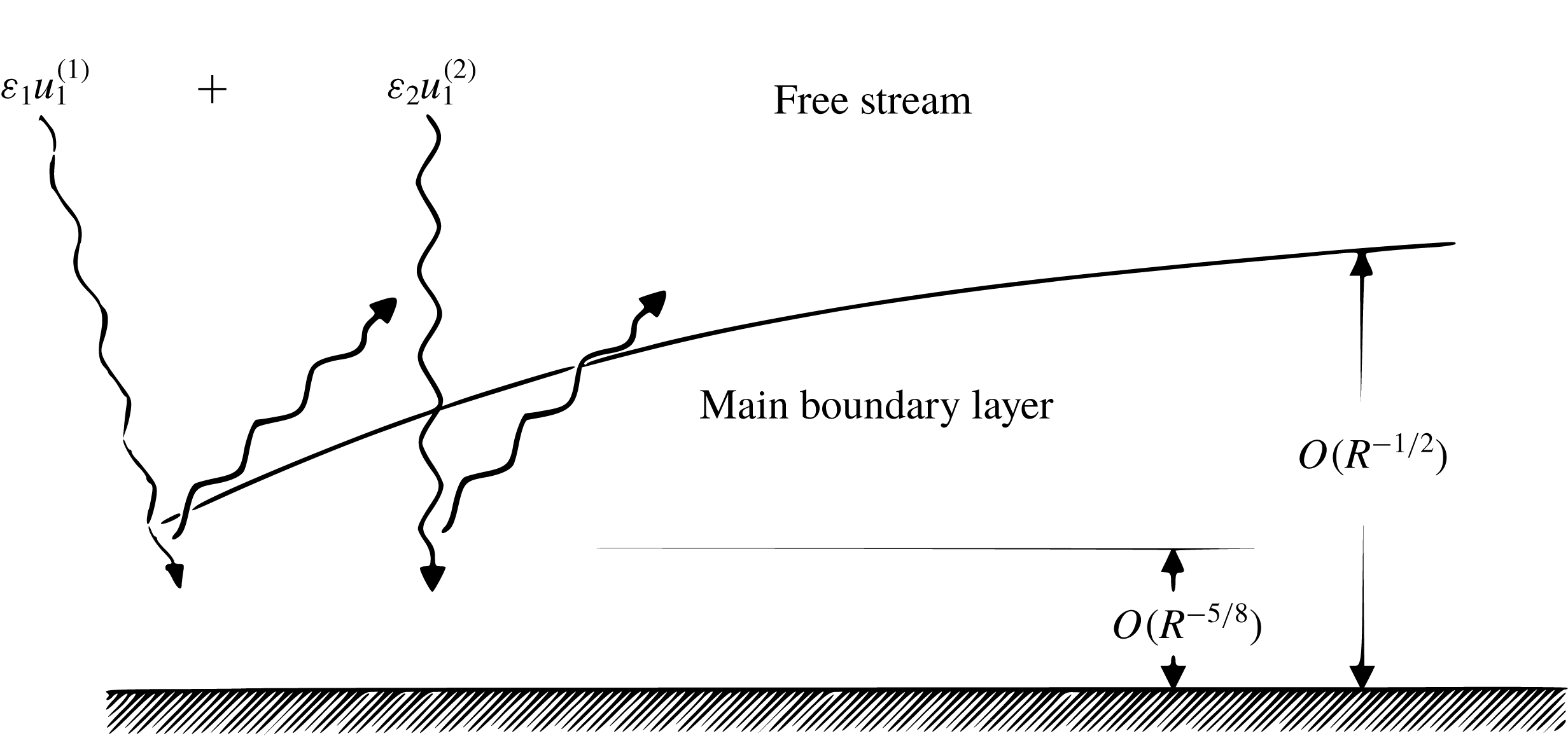
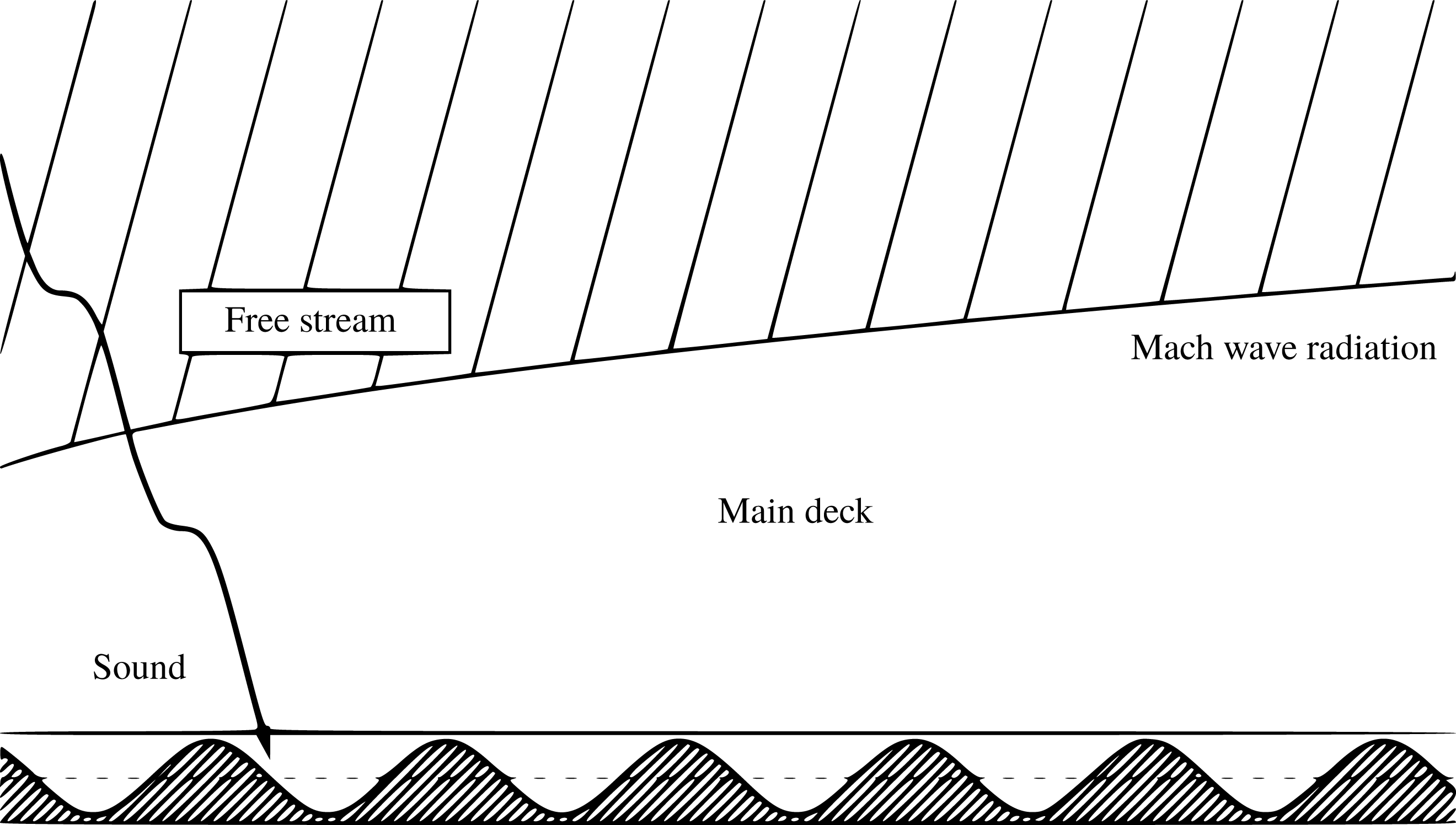
Sketch of the physical setting showing the impingement/penetration of two acoustic waves.

Suppose that two three-dimensional sound waves are present in the free stream (figure 1), and they are represented by
 $$\begin{eqnarray}\unicode[STIX]{x1D700}_{1}\text{e}^{\text{i}(\unicode[STIX]{x1D6FC}_{1}x+\unicode[STIX]{x1D6FD}_{1}z+\unicode[STIX]{x1D6FE}_{1}y-\unicode[STIX]{x1D714}_{1}t)}\quad \text{and}\quad \unicode[STIX]{x1D700}_{2}\text{e}^{\text{i}(\unicode[STIX]{x1D6FC}_{2}x+\unicode[STIX]{x1D6FD}_{2}z+\unicode[STIX]{x1D6FE}_{2}y-\unicode[STIX]{x1D714}_{2}t)}.\end{eqnarray}$$
From the dispersion relation obtained with the inviscid approximation, the phase speeds are
 $$\begin{eqnarray}c=\frac{\unicode[STIX]{x1D714}}{\unicode[STIX]{x1D6FC}}=1\pm \frac{\sqrt{\unicode[STIX]{x1D6FC}^{2}+\unicode[STIX]{x1D6FD}^{2}+\unicode[STIX]{x1D6FE}^{2}}}{\unicode[STIX]{x1D6FC}M},\end{eqnarray}$$
where the plus and minus signs stand for the fast/slow acoustic waves respectively, and
 $\unicode[STIX]{x1D6FC}$
,
 $\unicode[STIX]{x1D6FD}$
,
 $\unicode[STIX]{x1D6FE}$
and
 $c$
refer to
 $\unicode[STIX]{x1D6FC}_{j}$
,
 $\unicode[STIX]{x1D6FD}_{j}$
,
 $\unicode[STIX]{x1D6FE}_{j}$
and
 $c_{j}$
with
 $j=1,2$
. The dispersion relation may be written as
 $M(\unicode[STIX]{x1D714}-\unicode[STIX]{x1D6FC})=\pm (\unicode[STIX]{x1D6FC}^{2}+\unicode[STIX]{x1D6FD}^{2}+\unicode[STIX]{x1D6FE}^{2})^{1/2}$
, or equivalently
 $$\begin{eqnarray}(1-M^{2})\left[\unicode[STIX]{x1D6FC}-\frac{M^{2}\unicode[STIX]{x1D714}}{M^{2}-1}\right]^{2}+\unicode[STIX]{x1D6FD}^{2}+\unicode[STIX]{x1D6FE}^{2}=\frac{M^{2}\unicode[STIX]{x1D714}^{2}}{1-M^{2}},\end{eqnarray}$$
an equation representing a conic section for a given
 $\unicode[STIX]{x1D714}$
in the wavenumber space
 $(\unicode[STIX]{x1D6FC},\unicode[STIX]{x1D6FD},\unicode[STIX]{x1D6FE})$
: an ellipse if
 $M<1$
and a hyperbola when
 $M>1$
. The hyperbola consists of the left and right branches, which lie in the regions
 $\unicode[STIX]{x1D6FC}<M\unicode[STIX]{x1D714}/(M+1)$
and
 $\unicode[STIX]{x1D6FC}>M\unicode[STIX]{x1D714}/(M-1)$
respectively. The interaction between the two waves in (2.21) generates two forms of forcing proportional to
 $\text{e}^{\text{i}\{(\unicode[STIX]{x1D6FC}_{1}\pm \unicode[STIX]{x1D6FC}_{2})x+(\unicode[STIX]{x1D6FD}_{1}\pm \unicode[STIX]{x1D6FD}_{2})z-(\unicode[STIX]{x1D714}_{1}\pm \unicode[STIX]{x1D714}_{2})t\}}$
. The forcing from the sum/difference interactions, corresponding to the plus and minus signs, would be in resonance with a neutral T–S mode
 $\text{e}^{\text{i}\{\unicode[STIX]{x1D6FC}_{TS}x+\unicode[STIX]{x1D6FD}_{TS}z-\unicode[STIX]{x1D714}_{TS}t\}}$
if their wavenumbers and frequencies satisfy the relations
 $$\begin{eqnarray}\unicode[STIX]{x1D6FC}_{1}\pm \unicode[STIX]{x1D6FC}_{2}=\unicode[STIX]{x1D6FC}_{TS},\quad \unicode[STIX]{x1D6FD}_{1}\pm \unicode[STIX]{x1D6FD}_{2}=\unicode[STIX]{x1D6FD}_{TS},\quad \unicode[STIX]{x1D714}_{1}\pm \unicode[STIX]{x1D714}_{2}=\unicode[STIX]{x1D714}_{TS},\end{eqnarray}$$
which will be referred to as the resonance conditions. Our focus will be on first Mack modes, which have larger amplification rates than second Mack modes for
 $M<4.5$
, beyond which second modes become more unstable (Mack Reference Mack1984). In the lower-branch regime, first Mack modes have asymptotically small phase speeds, i.e.
 $\unicode[STIX]{x1D714}_{TS}\ll \unicode[STIX]{x1D6FC}_{TS}$
(in fact,
 $\unicode[STIX]{x1D714}_{TS}=O(R^{-1/8}\unicode[STIX]{x1D6FC}_{TS})$
, see below) at large
 $R$
. Typical sound waves have
 $O(1)$
phase speeds,
 $\unicode[STIX]{x1D714}_{j}=O(\unicode[STIX]{x1D6FC}_{j})$
and so
 $\unicode[STIX]{x1D714}_{1}+\unicode[STIX]{x1D714}_{2}=O(\unicode[STIX]{x1D6FC}_{1}+\unicode[STIX]{x1D6FC}_{2})$
. The required resonance conditions for the sum interaction cannot possibly be met for first Mack modes. The resonance conditions for the difference interaction can be satisfied by a pair of sound waves with
 $O(\unicode[STIX]{x1D6FC}_{1})=O(\unicode[STIX]{x1D6FC}_{2})=O(\unicode[STIX]{x1D6FC}_{TS})$
but nearly the same frequencies,
 $\unicode[STIX]{x1D714}_{1}$
and
 $\unicode[STIX]{x1D714}_{2}$
, suitably chosen such that
 $\unicode[STIX]{x1D714}_{1}-\unicode[STIX]{x1D714}_{2}=\unicode[STIX]{x1D714}_{TS}\ll \unicode[STIX]{x1D714}_{1},\unicode[STIX]{x1D714}_{2}$
. However, for sound waves with
 $c=O(1)$
, the induced signature in the boundary layer is of the same order of magnitude as in the free stream. They are less effective in generating first Mack modes that those with
 $c\ll 1$
or equivalently
 $\unicode[STIX]{x1D714}\ll \unicode[STIX]{x1D6FC}$
. It is however worth pointing out that the general mechanism of sound–sound interaction operates to excite second Mack modes as well; for example, the interaction of slow and fast sound waves does so, as was shown by DNS (Gao, Luo & Wu Reference Gao, Luo and Wu2015).
When
 $\unicode[STIX]{x1D714}\ll \unicode[STIX]{x1D6FC}$
, the dispersion relation (2.23) reduces to
 $\unicode[STIX]{x1D6FD}^{2}+\unicode[STIX]{x1D6FE}^{2}=(M^{2}-1)\unicode[STIX]{x1D6FC}^{2},$
which is possible only in the supersonic regime
 $M>1$
. It follows that the wavenumbers of the two interacting acoustic waves have to satisfy
 $$\begin{eqnarray}|\unicode[STIX]{x1D6FD}_{1}|<\unicode[STIX]{x1D6FC}_{1}\sqrt{M^{2}-1},\quad |\unicode[STIX]{x1D6FD}_{2}|<\unicode[STIX]{x1D6FC}_{2}\sqrt{M^{2}-1}.\end{eqnarray}$$
The difference interaction between the two slow acoustic waves can excite a T–S mode if (2.24) with the
 $-$
sign holds. For a T–S wave, its wavenumbers must satisfy (Smith Reference Smith1989)
 $$\begin{eqnarray}\unicode[STIX]{x1D6FD}_{TS}>\unicode[STIX]{x1D6FC}_{TS}\sqrt{M^{2}-1},\end{eqnarray}$$
which requires that
 $$\begin{eqnarray}\unicode[STIX]{x1D6FD}_{1}-\unicode[STIX]{x1D6FD}_{2}>(\unicode[STIX]{x1D6FC}_{1}-\unicode[STIX]{x1D6FC}_{2})\sqrt{M^{2}-1}.\end{eqnarray}$$
We will show that for any
 $(\unicode[STIX]{x1D6FC}_{TS},\unicode[STIX]{x1D6FD}_{TS})$
, it is always possible to find
 $(\unicode[STIX]{x1D6FC}_{1},\unicode[STIX]{x1D6FD}_{1})$
and
 $(\unicode[STIX]{x1D6FC}_{2},\unicode[STIX]{x1D6FD}_{2})$
to satisfy (2.24) and (2.27). In contrast, the forcing from the sum interaction cannot be in resonance since
 $\unicode[STIX]{x1D6FD}_{1}+\unicode[STIX]{x1D6FD}_{2}<(\unicode[STIX]{x1D6FC}_{1}+\unicode[STIX]{x1D6FC}_{2})\sqrt{M^{2}-1}$
, and is therefore discarded.
In summary, we focus on the difference interaction between sound waves with phase speeds
 $c_{j}=\unicode[STIX]{x1D714}_{j}/\unicode[STIX]{x1D6FC}_{j}\ll 1$
. The ensuing receptivity mechanism is very strong, as will be shown later. A finite-Reynolds-number formulation for the receptivity is possible but is left to the future. Here we take a high-Reynolds-number approach, which has the advantage of being mathematically consistent, probing into the detailed excitation process and giving explicit analytical results.
2.4 Asymptotic scalings
The lower-branch first Mack modes in a supersonic boundary layer have the characteristic scalings
 $\unicode[STIX]{x1D714}_{TS}=R^{1/4}\hat{\unicode[STIX]{x1D714}}_{TS}$
and
 $(\unicode[STIX]{x1D6FC}_{TS},\unicode[STIX]{x1D6FD}_{TS})=R^{3/8}(\hat{\unicode[STIX]{x1D6FC}}_{TS},\hat{\unicode[STIX]{x1D6FD}}_{TS})$
for the frequency and wavenumbers (Smith Reference Smith1989), the same as the T–S waves in the incompressible regime. In the present paper, we assume that the two sound waves are both on the triple-deck scale, and thus their wavenumbers and frequencies are scaled as
 $$\begin{eqnarray}(\unicode[STIX]{x1D6FC}_{j},\unicode[STIX]{x1D6FD}_{j})=R^{3/8}C^{-3/8}\unicode[STIX]{x1D70F}_{w}^{-3/2}(\hat{\unicode[STIX]{x1D6FC}}_{j},\hat{\unicode[STIX]{x1D6FD}}_{j}),\quad \unicode[STIX]{x1D714}_{j}=R^{2/8}C^{-1/4}\unicode[STIX]{x1D70F}_{w}^{-1}\hat{\unicode[STIX]{x1D714}}_{j},\quad (j=1,2).\end{eqnarray}$$
Note that the phase speed
 $c_{j}=O(R^{-1/8})$
, which is what a ‘slow acoustic wave’ means precisely in the present paper. In terms of the rescaled quantities
 $\hat{\unicode[STIX]{x1D6FC}}_{j}$
,
 $\hat{\unicode[STIX]{x1D6FD}}_{j}$
and
 $\hat{\unicode[STIX]{x1D714}}_{j}$
, the resonance conditions (2.24) for the difference interaction are expressed as
 $$\begin{eqnarray}\hat{\unicode[STIX]{x1D6FC}}_{1}-\hat{\unicode[STIX]{x1D6FC}}_{2}=\hat{\unicode[STIX]{x1D6FC}}_{TS},\quad \hat{\unicode[STIX]{x1D6FD}}_{1}-\hat{\unicode[STIX]{x1D6FD}}_{2}=\hat{\unicode[STIX]{x1D6FD}}_{TS},\quad \hat{\unicode[STIX]{x1D714}}_{1}-\hat{\unicode[STIX]{x1D714}}_{2}=\hat{\unicode[STIX]{x1D714}}_{TS}.\end{eqnarray}$$
In view of (2.28), we introduce the time, streamwise and spanwise variables
 $$\begin{eqnarray}\bar{t}=R^{2/8}C^{-1/4}\unicode[STIX]{x1D70F}_{w}^{-1}t,\quad \bar{x}=R^{3/8}C^{-3/8}\unicode[STIX]{x1D70F}_{w}^{-3/2}x,\quad \bar{z}=R^{3/8}C^{-3/8}\unicode[STIX]{x1D70F}_{w}^{-3/2}z.\end{eqnarray}$$
The impingement of each sound wave is also described by the triple-deck theory, which allows us to calculate the reflection coefficient and the signature induced in the boundary layer.
Since the unsteady fluctuation driven by the acoustic pressure acquires
 $O(\unicode[STIX]{x1D700}_{s}R^{1/8})$
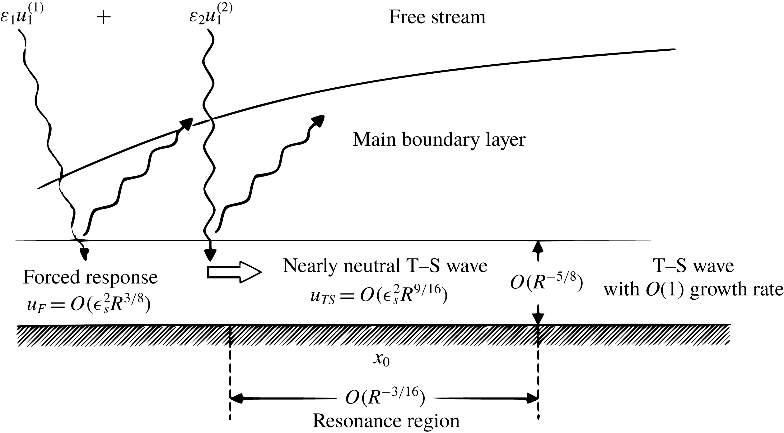
in the lower deck, the dominant interaction between the two impinging sound waves takes place there. As was first pointed out by Wu (Reference Wu1999) for the vortical–sound interaction, the forced response evolves into a T–S mode on approaching the neutral point,
 $x_{0}$
, where the resonance conditions in (2.29) are met. In order to describe this change of the character, it is necessary to include the non-parallel-flow effect, which becomes important in an
 $O(\bar{\unicode[STIX]{x1D700}})$
neighbourhood of
 $x_{0}$
, where
 $\bar{\unicode[STIX]{x1D700}}=R^{-3/16}C^{3/16}\unicode[STIX]{x1D70F}_{w}^{3/4}$
(Ruban Reference Ruban1983; Hall & Smith Reference Hall and Smith1984). The evolution of the forced response to an eigenmode is described by the variable (Wu Reference Wu1999)
 $$\begin{eqnarray}x_{1}=(x-x_{0})/\bar{\unicode[STIX]{x1D700}},\end{eqnarray}$$
and the amplitude of the T–S wave will be a function of
 $x_{1}$
. We may set
 $x_{0}=1$
by taking
 $L$
to be the distance from the neutral point to the leading edge. The wall shear stress of the base flow,
 $\unicode[STIX]{x1D706}=\unicode[STIX]{x1D706}_{0}x^{-1/2}$
, is therefore expanded about
 $x_{0}=1$
as
 $$\begin{eqnarray}\unicode[STIX]{x1D706}=\unicode[STIX]{x1D706}_{0}+\bar{\unicode[STIX]{x1D700}}\unicode[STIX]{x1D706}_{1}x_{1}\quad \text{with}~\unicode[STIX]{x1D706}_{1}=-\unicode[STIX]{x1D706}_{0}/2.\end{eqnarray}$$
2.5 Upper deck
The transverse extent of the upper deck is
 $O(R^{-3/8}L)$
, and thus a wall-normal variable
 $\bar{y}=R^{-1/8}C^{-3/8}\unicode[STIX]{x1D70F}_{w}^{-3/2}y$
is introduced. The mean flow is
 $(U_{B},V_{B},W_{B},P_{B},R_{B},T_{B})=(1,0,0,1/\unicode[STIX]{x1D6FE}M^{2},1,1)$
, and the expansion for the perturbation takes the form
 $$\begin{eqnarray}\displaystyle & \tilde{\boldsymbol{u}}=\unicode[STIX]{x1D700}_{s}\boldsymbol{u}_{1}+\unicode[STIX]{x1D700}_{s}^{2}\bar{\unicode[STIX]{x1D700}}^{-1}R^{2/8}(\boldsymbol{u}_{TS}E_{TS}+\text{c.c.})+\unicode[STIX]{x1D700}_{s}^{2}R^{2/8}\boldsymbol{u}_{2}+\cdots , & \displaystyle\end{eqnarray}$$
 $$\begin{eqnarray}\displaystyle & \tilde{p}=\unicode[STIX]{x1D700}_{s}p_{1}+\unicode[STIX]{x1D700}_{s}^{2}\bar{\unicode[STIX]{x1D700}}^{-1}R^{2/8}(p_{TS}E_{TS}+\text{c.c.})+\unicode[STIX]{x1D700}_{s}^{2}R^{2/8}p_{2}+\cdots , & \displaystyle\end{eqnarray}$$
 $$\begin{eqnarray}\displaystyle & \tilde{\unicode[STIX]{x1D70C}}=\unicode[STIX]{x1D700}_{s}\unicode[STIX]{x1D70C}_{1}+\unicode[STIX]{x1D700}_{s}^{2}\bar{\unicode[STIX]{x1D700}}^{-1}R^{2/8}(\unicode[STIX]{x1D70C}_{TS}E_{TS}+\text{c.c.})+\unicode[STIX]{x1D700}_{s}^{2}R^{2/8}\unicode[STIX]{x1D70C}_{2}+\cdots , & \displaystyle\end{eqnarray}$$
 $$\begin{eqnarray}\displaystyle & \tilde{\unicode[STIX]{x1D70F}}=\unicode[STIX]{x1D700}_{s}\unicode[STIX]{x1D70F}_{1}+\unicode[STIX]{x1D700}_{s}^{2}\bar{\unicode[STIX]{x1D700}}^{-1}R^{2/8}(\unicode[STIX]{x1D70F}_{TS}E_{TS}+\text{c.c.})+\unicode[STIX]{x1D700}_{s}^{2}R^{2/8}\unicode[STIX]{x1D70F}_{2}+\cdots , & \displaystyle\end{eqnarray}$$
where
 $$\begin{eqnarray}E_{TS}=\exp \{\text{i}(\hat{\unicode[STIX]{x1D6FC}}_{TS}\bar{x}+\hat{\unicode[STIX]{x1D6FD}}_{TS}\bar{z}-\hat{\unicode[STIX]{x1D714}}_{TS}\bar{t})\},\end{eqnarray}$$
and we remind the reader that
 $\unicode[STIX]{x1D700}_{1}=\unicode[STIX]{x1D700}_{2}=\unicode[STIX]{x1D700}_{s}$
has been chosen without loss of generality. The
 $O(\unicode[STIX]{x1D700}_{s})$
terms represent the impinging and reflected sound waves. The
 $O(\unicode[STIX]{x1D700}_{s}^{2}R^{2/8})$
terms represent the upper-deck signature of the perturbation forced by the sound–sound interaction in the lower deck; these terms are greater than
 $O(\unicode[STIX]{x1D700}_{s}^{2})$
terms which would be generated by the sound–sound interaction in the upper deck. Due to the resonant nature of the forcing, the T–S mode excited has a magnitude larger by a factor
 $\bar{\unicode[STIX]{x1D700}}^{-1}=O(R^{3/16})$
.
2.5.1 Leading order
Substitution of (2.33)–(2.36) along with the base flow and (2.30) into (2.13)–(2.18) yields, at
 $O(\unicode[STIX]{x1D700}_{s})$
, the linearized equations,
 $$\begin{eqnarray}\frac{\unicode[STIX]{x2202}\unicode[STIX]{x1D70C}_{1}}{\unicode[STIX]{x2202}\bar{x}}+\unicode[STIX]{x1D735}\boldsymbol{\cdot }\boldsymbol{u}_{1}=0,\quad \frac{\unicode[STIX]{x2202}\boldsymbol{u}_{1}}{\unicode[STIX]{x2202}\bar{x}}=-\unicode[STIX]{x1D735}p_{1},\quad \frac{\unicode[STIX]{x2202}\unicode[STIX]{x1D70F}_{1}}{\unicode[STIX]{x2202}\bar{x}}=(\unicode[STIX]{x1D6FE}-1)M^{2}\frac{\unicode[STIX]{x2202}p_{1}}{\unicode[STIX]{x2202}\bar{x}},\end{eqnarray}$$
 $$\begin{eqnarray}\unicode[STIX]{x1D6FE}M^{2}p_{1}=\unicode[STIX]{x1D70F}_{1}+\unicode[STIX]{x1D70C}_{1}.\end{eqnarray}$$
Note that for perturbations with
 $O(R^{2/8})$
frequency and
 $O(R^{3/8})$
wavenumbers, their governing equations in the upper deck are quasi-steady. Equations (2.38)–(2.39) can be combined to obtain an equation for the pressure
 $p_{1}$
,
 $$\begin{eqnarray}M^{2}\frac{\unicode[STIX]{x2202}^{2}p_{1}}{\unicode[STIX]{x2202}\bar{x}^{2}}-\unicode[STIX]{x1D6FB}^{2}p_{1}=0,\end{eqnarray}$$
where the operators
 $\unicode[STIX]{x1D735}$
and
 $\unicode[STIX]{x1D6FB}^{2}$
have been defined with respect to the upper-deck variables
 $\bar{x}$
,
 $\bar{y}$
and
 $\bar{z}$
.
The solution for
 $\boldsymbol{u}_{1}$
,
 $p_{1}$
,
 $\unicode[STIX]{x1D70C}_{1}$
and
 $\unicode[STIX]{x1D70F}_{1}$
can be expressed as the sum of two acoustic modes,
 $$\begin{eqnarray}\boldsymbol{u}_{1}=\boldsymbol{u}_{1}^{(1)}+\boldsymbol{u}_{1}^{(2)},\quad p_{1}=p_{1}^{(1)}+p_{1}^{(2)},\quad \unicode[STIX]{x1D70C}_{1}=\unicode[STIX]{x1D70C}_{1}^{(1)}+\unicode[STIX]{x1D70C}_{1}^{(2)},\quad \unicode[STIX]{x1D70F}_{1}=\unicode[STIX]{x1D70F}_{1}^{(1)}+\unicode[STIX]{x1D70F}_{1}^{(2)},\end{eqnarray}$$
where we assume the solution to be of the travelling-wave form, namely
 $$\begin{eqnarray}(\boldsymbol{u}_{1}^{(j)},p_{1}^{(j)},\unicode[STIX]{x1D70C}_{1}^{(j)},\unicode[STIX]{x1D70F}_{1}^{(j)})=(\hat{\boldsymbol{u}}_{1}^{(j)},\hat{p}_{1}^{(j)},\hat{\unicode[STIX]{x1D70C}}_{1}^{(j)},\hat{\unicode[STIX]{x1D70F}}_{1}^{(j)})E_{j}+\text{c.c.}\quad \text{with}~E_{j}=\text{e}^{\text{i}(\hat{\unicode[STIX]{x1D6FC}}_{j}\bar{x}+\hat{\unicode[STIX]{x1D6FD}}_{j}\bar{z}-\hat{\unicode[STIX]{x1D714}}_{j}\bar{t})}.\end{eqnarray}$$
In order to allow for wave reflection,
 $\hat{p}_{1}^{(j)}$
will take the form
 $$\begin{eqnarray}\hat{p}_{1}^{(j)}=p_{a}^{(j)}(\text{e}^{\text{i}\hat{\unicode[STIX]{x1D6FE}}_{j}\bar{y}}+{\mathcal{R}}^{(j)}\text{e}^{-\text{i}\hat{\unicode[STIX]{x1D6FE}}_{j}\bar{y}}),\end{eqnarray}$$
where the first term represents the incident wave and the second the reflected wave, and
 ${\mathcal{R}}^{(j)}$
is the reflection coefficient to be found as part of the solution. In the following analysis, we will take
 $p_{a}^{(j)}=1$
without losing generality. Substituting
 $p_{1}^{(j)}$
into (2.40) yields a relationship for the wavenumbers
 $$\begin{eqnarray}(M^{2}-1)\hat{\unicode[STIX]{x1D6FC}}_{j}^{2}-\hat{\unicode[STIX]{x1D6FD}}_{j}^{2}-\hat{\unicode[STIX]{x1D6FE}}_{j}^{2}=0.\end{eqnarray}$$
The matching condition with the main-deck solution reads
 $$\begin{eqnarray}\frac{\unicode[STIX]{x2202}p_{1}}{\unicode[STIX]{x2202}\bar{y}}=-\frac{\unicode[STIX]{x2202}v_{1}}{\unicode[STIX]{x2202}\bar{x}}\quad \text{at}~\bar{y}=0,\end{eqnarray}$$
where
 $v_{1}$
will be given by the so-called outer limit of the main-deck solution.
2.5.2 T–S wave
Working with the
 $O(\unicode[STIX]{x1D700}_{s}^{2}\bar{\unicode[STIX]{x1D700}}^{-1}R^{2/8})$
terms in (2.33)–(2.36), we obtain the equations governing the T–S wave,
 $$\begin{eqnarray}\frac{\unicode[STIX]{x2202}^{2}p_{TS}}{\unicode[STIX]{x2202}\bar{y}^{2}}-\hat{\unicode[STIX]{x1D6FE}}_{TS}^{2}p_{TS}=0,\quad \text{i}\hat{\unicode[STIX]{x1D6FC}}_{TS}v_{TS}=-\frac{\unicode[STIX]{x2202}p_{TS}}{\unicode[STIX]{x2202}\bar{y}},\end{eqnarray}$$
where
 $\hat{\unicode[STIX]{x1D6FE}}_{TS}^{2}=(1-M^{2})\hat{\unicode[STIX]{x1D6FC}}_{TS}^{2}+\hat{\unicode[STIX]{x1D6FD}}_{TS}^{2}$
. The solution is found as
 $$\begin{eqnarray}p_{TS}=\hat{p}_{TS}A(x_{1})\text{e}^{-\hat{\unicode[STIX]{x1D6FE}}_{TS}\bar{y}},\quad v_{TS}=-\text{i}\frac{\hat{\unicode[STIX]{x1D6FE}}_{TS}}{\hat{\unicode[STIX]{x1D6FC}}_{TS}}\hat{p}_{TS}A(x_{1})\text{e}^{-\hat{\unicode[STIX]{x1D6FE}}_{TS}\bar{y}},\end{eqnarray}$$
where
 $A(x_{1})$
is the amplitude of the T–S wave. The main mathematical task is to derive the evolution equation for
 $A(x_{1})$
. This will be done by analysing the solution at the next order, which represents the response to the sound–sound interaction. The reader may in the first reading skip the technical details, and turn directly to the key results of physical relevance, which include the reflection coefficient (2.85), the acoustic signature in the boundary layer, equations (2.88)–(2.89) and (2.91), the dispersion relation for the instability (2.97) and the final amplitude equation (2.116).
2.5.3 Response in the upper deck
At
 $O(\unicode[STIX]{x1D700}_{s}^{2}R^{2/8})$
, the equations are
 $$\begin{eqnarray}\displaystyle & \displaystyle \frac{\unicode[STIX]{x2202}\unicode[STIX]{x1D70C}_{2}}{\unicode[STIX]{x2202}\bar{x}}+\unicode[STIX]{x1D735}\boldsymbol{\cdot }\boldsymbol{u}_{2}=-\left(\frac{\unicode[STIX]{x2202}\unicode[STIX]{x1D70C}_{TS}}{\unicode[STIX]{x2202}x_{1}}+\frac{\unicode[STIX]{x2202}u_{TS}}{\unicode[STIX]{x2202}x_{1}}\right)E_{TS}, & \displaystyle\end{eqnarray}$$
 $$\begin{eqnarray}\displaystyle & \displaystyle \frac{\unicode[STIX]{x2202}\boldsymbol{u}_{2}}{\unicode[STIX]{x2202}\bar{x}}=-\unicode[STIX]{x1D735}p_{2}+\left(\frac{-\unicode[STIX]{x2202}\boldsymbol{u}_{TS}}{\unicode[STIX]{x2202}x_{1}}-\frac{\unicode[STIX]{x2202}p_{TS}}{\unicode[STIX]{x2202}x_{1}}\boldsymbol{i}\right)E_{TS}, & \displaystyle\end{eqnarray}$$
 $$\begin{eqnarray}\displaystyle & \displaystyle \frac{\unicode[STIX]{x2202}\unicode[STIX]{x1D70F}_{2}}{\unicode[STIX]{x2202}\bar{x}}=-\frac{\unicode[STIX]{x2202}\unicode[STIX]{x1D70F}_{TS}}{\unicode[STIX]{x2202}x_{1}}E_{TS}+(\unicode[STIX]{x1D6FE}-1)M^{2}\frac{\unicode[STIX]{x2202}p_{2}}{\unicode[STIX]{x2202}\bar{x}}+(\unicode[STIX]{x1D6FE}-1)M^{2}\frac{\unicode[STIX]{x2202}p_{TS}}{\unicode[STIX]{x2202}x_{1}}E_{TS}, & \displaystyle\end{eqnarray}$$
 $$\begin{eqnarray}\displaystyle & \displaystyle \unicode[STIX]{x1D6FE}M^{2}p_{2}=\unicode[STIX]{x1D70F}_{2}+\unicode[STIX]{x1D70C}_{2}. & \displaystyle\end{eqnarray}$$
Elimination of
 $\boldsymbol{u}_{2}$
,
 $\unicode[STIX]{x1D70F}_{2}$
and
 $\unicode[STIX]{x1D70C}_{2}$
among (2.48)–(2.51) gives the equation for
 $p_{2}$
,
 $$\begin{eqnarray}M^{2}\frac{\unicode[STIX]{x2202}^{2}p_{2}}{\unicode[STIX]{x2202}\bar{x}^{2}}-\unicode[STIX]{x1D6FB}^{2}p_{2}=2\text{i}(1-M^{2})\hat{\unicode[STIX]{x1D6FC}}_{TS}A^{\prime }(x_{1})\hat{p}_{TS}\text{e}^{-\hat{\unicode[STIX]{x1D6FE}}_{TS}\bar{y}}E_{TS}.\end{eqnarray}$$
The solution for
 $p_{2}$
takes the form
 $p_{2}=(\hat{P}_{2}(\bar{y})E_{TS}+\text{c.c.})$
, where
 $$\begin{eqnarray}\hat{P}_{2}=\left\{\hat{p}_{2}+\frac{\text{i}\hat{\unicode[STIX]{x1D6FC}}_{TS}}{\hat{\unicode[STIX]{x1D6FE}}_{TS}}(1-M^{2})A^{\prime }\bar{y}\right\}\text{e}^{-\hat{\unicode[STIX]{x1D6FE}}_{TS}\bar{y}},\end{eqnarray}$$
with
 $\hat{p}_{2}$
being an arbitrary function of
 $x_{1}$
. The vertical velocity
 $v_{2}$
can readily be obtained from the vertical momentum equation in (2.49) after substituting
 $p_{2}$
, but it suffices to note that as
 $\bar{y}\rightarrow 0$
,
 $$\begin{eqnarray}\displaystyle & p_{2}\rightarrow \hat{p}_{2}E_{TS}, & \displaystyle\end{eqnarray}$$
 $$\begin{eqnarray}\displaystyle & \displaystyle v_{2}\rightarrow \left(-\frac{(1-M^{2})}{\hat{\unicode[STIX]{x1D6FE}}_{TS}}A^{\prime }\hat{p}_{TS}+\frac{\hat{\unicode[STIX]{x1D6FE}}_{TS}}{\text{i}\hat{\unicode[STIX]{x1D6FC}}_{TS}}\hat{p}_{2}+\frac{\hat{\unicode[STIX]{x1D6FE}}_{TS}}{\hat{\unicode[STIX]{x1D6FC}}_{TS}^{2}}A^{\prime }\hat{p}_{TS}\right)E_{TS}. & \displaystyle\end{eqnarray}$$
2.6 Main deck
The transverse variable is now
 ${\tilde{y}}=C^{-1/2}\unicode[STIX]{x1D70F}_{w}^{-1}y=O(1)$
and the expansion for the perturbation takes the form
 $$\begin{eqnarray}\displaystyle & \tilde{u} =C^{1/8}\unicode[STIX]{x1D70F}_{w}^{1/2}[\unicode[STIX]{x1D700}_{s}R^{1/8}(\hat{u} _{1}^{(1)}E_{1}+\hat{u} _{1}^{(2)}E_{2})+\unicode[STIX]{x1D700}_{s}^{2}\bar{\unicode[STIX]{x1D700}}^{-1}R^{3/8}\tilde{u} _{TS}+\unicode[STIX]{x1D700}_{s}^{2}R^{3/8}\hat{u} _{2}E_{TS}+\cdots ], & \displaystyle\end{eqnarray}$$
 $$\begin{eqnarray}\displaystyle & \tilde{v}=C^{1/4}[\unicode[STIX]{x1D700}_{s}(\hat{v}_{1}^{(1)}E_{1}+\hat{v}_{1}^{(2)}E_{2})+\unicode[STIX]{x1D700}_{s}^{2}\bar{\unicode[STIX]{x1D700}}^{-1}R^{2/8}\tilde{v}_{TS}+\unicode[STIX]{x1D700}_{s}^{2}R^{2/8}\hat{v}_{2}E_{TS}+\cdots ], & \displaystyle\end{eqnarray}$$
 $$\begin{eqnarray}\displaystyle & \tilde{w}=C^{1/4}\unicode[STIX]{x1D70F}_{w}[\unicode[STIX]{x1D700}_{s}({\hat{w}}_{1}^{(1)}E_{1}+{\hat{w}}_{1}^{(2)}E_{2})+\unicode[STIX]{x1D700}_{s}^{2}\bar{\unicode[STIX]{x1D700}}^{-1}R^{2/8}\tilde{w}_{TS}+\unicode[STIX]{x1D700}_{s}^{2}R^{2/8}{\hat{w}}_{2}E_{TS}+\cdots ], & \displaystyle\end{eqnarray}$$
 $$\begin{eqnarray}\displaystyle & \tilde{p}=C^{1/4}[\unicode[STIX]{x1D700}_{s}(\hat{p}_{1}^{(1)}E_{1}+\hat{p}_{1}^{(2)}E_{2})+\unicode[STIX]{x1D700}_{s}^{2}\bar{\unicode[STIX]{x1D700}}^{-1}R^{2/8}\tilde{p}_{TS}+\unicode[STIX]{x1D700}_{s}^{2}R^{2/8}\hat{p}_{2}E_{TS}+\cdots ], & \displaystyle\end{eqnarray}$$
 $$\begin{eqnarray}\displaystyle & \tilde{\unicode[STIX]{x1D70C}}=C^{1/8}\unicode[STIX]{x1D70F}_{w}^{1/2}[\unicode[STIX]{x1D700}_{s}R^{1/8}(\hat{R}_{1}^{(1)}E_{1}+\hat{R}_{1}^{(2)}E_{2})+\unicode[STIX]{x1D700}_{s}^{2}\bar{\unicode[STIX]{x1D700}}^{-1}R^{3/8}\tilde{R}_{TS}+\unicode[STIX]{x1D700}_{s}^{2}R^{3/8}\hat{R}_{2}E_{TS}+\cdots ], & \displaystyle\end{eqnarray}$$
 $$\begin{eqnarray}\displaystyle & \tilde{\unicode[STIX]{x1D70F}}=C^{1/8}\unicode[STIX]{x1D70F}_{w}^{1/2}[\unicode[STIX]{x1D700}_{s}R^{1/8}(\hat{\unicode[STIX]{x1D70F}}_{1}^{(1)}E_{1}+\hat{\unicode[STIX]{x1D70F}}_{1}^{(2)}E_{2})+\unicode[STIX]{x1D700}_{s}^{2}\bar{\unicode[STIX]{x1D700}}^{-1}R^{3/8}\tilde{\unicode[STIX]{x1D70F}}_{TS}+\unicode[STIX]{x1D700}_{s}^{2}R^{3/8}\hat{\unicode[STIX]{x1D70F}}_{2}E_{TS}+\cdots ]. & \displaystyle\end{eqnarray}$$
2.6.1 Leading order
Inserting (2.56)–(2.61) into (2.13)–(2.18), we obtain at leading order
 $O(\unicode[STIX]{x1D700}_{s}R^{1/8})$
the equations,
 $$\begin{eqnarray}\left.\begin{array}{@{}c@{}}\displaystyle \text{i}\hat{\unicode[STIX]{x1D6FC}}_{1}U_{B}\hat{R}_{1}+\text{i}\hat{\unicode[STIX]{x1D6FC}}_{1}R_{B}\hat{u} _{1}+R_{B}^{\prime }\hat{v}_{1}+R_{B}\frac{\unicode[STIX]{x2202}\hat{v}_{1}}{\unicode[STIX]{x2202}{\tilde{y}}}=0,\\ \displaystyle \text{i}\hat{\unicode[STIX]{x1D6FC}}_{1}U_{B}\hat{u} _{1}+U_{B}^{\prime }\hat{v}_{1}=0,\quad \text{i}\hat{\unicode[STIX]{x1D6FC}}_{1}R_{B}U_{B}{\hat{w}}_{1}=-\text{i}\hat{\unicode[STIX]{x1D6FD}}_{1}\hat{p}_{1},\quad \text{i}\hat{\unicode[STIX]{x1D6FC}}_{1}U_{B}\hat{R}_{1}+R_{B}^{\prime }\hat{v}_{1}=0,\end{array}\right\}\end{eqnarray}$$
whose solution is
 $$\begin{eqnarray}\left.\begin{array}{@{}c@{}}\hat{u} _{1}=\hat{A}_{1}U_{B}^{\prime },\quad \hat{v}_{1}=-\text{i}\hat{\unicode[STIX]{x1D6FC}}\hat{A}_{1}U_{B},\quad {\hat{w}}_{1}=-(\hat{\unicode[STIX]{x1D6FD}}_{1}/\hat{\unicode[STIX]{x1D6FC}}_{1})\hat{p}_{1}/(R_{B}U_{B}),\\ \hat{R}_{1}=\hat{A}_{1}R_{B}^{\prime },\quad \hat{\unicode[STIX]{x1D70F}}_{1}=-\hat{A}_{1}R_{B}^{\prime }/R_{B}^{2},\end{array}\right\}\end{eqnarray}$$
where we have used the state equation to obtain
 $\unicode[STIX]{x1D70F}_{1}$
. The matching condition (2.45) gives
 $$\begin{eqnarray}\text{i}\hat{\unicode[STIX]{x1D6FE}}_{1}(1-{\mathcal{R}}^{(1)})=-\hat{\unicode[STIX]{x1D6FC}}_{1}^{2}\hat{A}_{1}.\end{eqnarray}$$
The streamwise and normal velocities of the T–S wave are,
 $$\begin{eqnarray}\tilde{u} _{TS}=BU_{B}^{\prime }({\tilde{y}})E_{TS}+\text{c.c.},\quad \tilde{v}_{TS}=-\frac{\unicode[STIX]{x2202}}{\unicode[STIX]{x2202}\bar{x}}(BU_{B}({\tilde{y}})E_{TS}+\text{c.c.}),\end{eqnarray}$$
where
 $\unicode[STIX]{x2202}/\unicode[STIX]{x2202}\bar{x}\rightarrow \unicode[STIX]{x2202}/\unicode[STIX]{x2202}\bar{x}+\bar{\unicode[STIX]{x1D700}}(\unicode[STIX]{x2202}/\unicode[STIX]{x2202}x_{1})$
. The displacement function
 $B$
must be expanded as (Wu Reference Wu1999)
 $$\begin{eqnarray}B=A(x_{1})B_{1}+\bar{\unicode[STIX]{x1D700}}B_{2}(x_{1}),\end{eqnarray}$$
so that the matching with the upper-deck solution can be carried out. The inner and outer limits of the main-deck solution (2.65) are then
 $$\begin{eqnarray}\displaystyle & \tilde{u} _{TS}\rightarrow [\unicode[STIX]{x1D706}_{0}AB_{1}+\bar{\unicode[STIX]{x1D700}}(\unicode[STIX]{x1D706}_{1}x_{1}AB_{1}+\unicode[STIX]{x1D706}_{0}B_{2})]E_{TS}+\text{c.c.}\quad \text{as}~{\tilde{y}}\rightarrow 0, & \displaystyle\end{eqnarray}$$
 $$\begin{eqnarray}\displaystyle & \tilde{v}_{TS}\rightarrow -[\text{i}\hat{\unicode[STIX]{x1D6FC}}_{TS}AB_{1}+\bar{\unicode[STIX]{x1D700}}(A^{\prime }B_{1}+\text{i}\hat{\unicode[STIX]{x1D6FC}}_{TS}B_{2})]E_{TS}+\text{c.c.}\quad \text{as}~{\tilde{y}}\rightarrow \infty . & \displaystyle\end{eqnarray}$$
Noting that
 $\tilde{p}_{TS}=\hat{P}_{TS}E_{TS}$
, and matching the upper-deck solutions (2.47) and (2.55) with the leading-order and second terms of the main-deck solution (2.68) respectively, we have,
 $$\begin{eqnarray}\displaystyle & \hat{\unicode[STIX]{x1D6FE}}_{TS}\hat{P}_{TS}=\hat{\unicode[STIX]{x1D6FC}}_{TS}^{2}B_{1}, & \displaystyle\end{eqnarray}$$
 $$\begin{eqnarray}\displaystyle & \displaystyle \hat{\unicode[STIX]{x1D6FC}}_{TS}^{2}B_{2}-2\text{i}\hat{\unicode[STIX]{x1D6FC}}_{TS}A^{\prime }(x_{1})B_{1}=\hat{\unicode[STIX]{x1D6FE}}_{TS}\hat{P}_{2}-\text{i}\frac{\hat{\unicode[STIX]{x1D6FC}}_{TS}}{\hat{\unicode[STIX]{x1D6FE}}_{TS}}(1-M^{2})A^{\prime }(x_{1})\hat{P}_{TS}. & \displaystyle\end{eqnarray}$$
2.7 Lower deck
The wall-normal variable is
 $Y=R^{1/8}C^{-5/8}\unicode[STIX]{x1D70F}_{w}^{-3/2}y$
. The base flow is approximated as
 $$\begin{eqnarray}U_{B}(Y)=R^{-1/8}C^{1/8}\unicode[STIX]{x1D70F}_{w}^{1/2}(\unicode[STIX]{x1D706}_{0}+\bar{\unicode[STIX]{x1D700}}\unicode[STIX]{x1D706}_{1}x_{1})Y+\cdots .\end{eqnarray}$$
The expansion takes the form
 $$\begin{eqnarray}\displaystyle & \tilde{u} =C^{1/8}\unicode[STIX]{x1D70F}_{w}^{1/2}[\unicode[STIX]{x1D700}_{s}R^{1/8}(\hat{U} _{1}^{(1)}E_{1}+\hat{U} _{1}^{(2)}E_{2})+\unicode[STIX]{x1D700}_{s}^{2}R^{3/8}(\bar{\unicode[STIX]{x1D700}}^{-1}A(x_{1})\hat{U} _{TS}+\hat{U} _{2})E_{TS}+\cdots ],\qquad & \displaystyle\end{eqnarray}$$
 $$\begin{eqnarray}\displaystyle & \tilde{v}=C^{3/8}\unicode[STIX]{x1D70F}_{w}^{1/2}[\unicode[STIX]{x1D700}_{s}R^{-1/8}(\hat{V}_{1}^{(1)}E_{1}+\hat{V}_{1}^{(2)}E_{2})+\unicode[STIX]{x1D700}_{s}^{2}R^{1/8}(\bar{\unicode[STIX]{x1D700}}^{-1}A(x_{1})\hat{V}_{TS}+\hat{V}_{2})E_{TS}+\cdots ],\qquad & \displaystyle\end{eqnarray}$$
 $$\begin{eqnarray}\displaystyle & \tilde{w}=C^{1/8}\unicode[STIX]{x1D70F}_{w}^{1/2}[\unicode[STIX]{x1D700}_{s}R^{1/8}({\hat{W}}_{1}^{(1)}E_{1}+{\hat{W}}_{1}^{(2)}E_{2})+\unicode[STIX]{x1D700}_{s}^{2}R^{3/8}(\bar{\unicode[STIX]{x1D700}}^{-1}A(x_{1}){\hat{W}}_{TS}+{\hat{W}}_{2})E_{TS}+\cdots ],\qquad & \displaystyle\end{eqnarray}$$
 $$\begin{eqnarray}\displaystyle & \tilde{p}=C^{1/4}[\unicode[STIX]{x1D700}_{s}(\hat{P}_{1}^{(1)}E_{1}+\hat{P}_{1}^{(2)}E_{2})+\unicode[STIX]{x1D700}_{s}^{2}R^{2/8}(\bar{\unicode[STIX]{x1D700}}^{-1}A(x_{1})\hat{P}_{TS}+\hat{P}_{2})E_{TS}+\cdots ].\qquad & \displaystyle\end{eqnarray}$$
The temperature and density disturbances are not considered since it is well known that in the lower deck they do not enter the continuity and momentum equations at leading order. The solution for each term in the expansion (2.72)–(2.75) is now considered.
2.7.1 Signature of sound waves
The leading-order terms in (2.72)–(2.75) represent the unsteady fluctuation driven by the sound waves. It is important to note that the streamwise and spanwise velocities are of
 $O(\unicode[STIX]{x1D700}_{s}R^{1/8})$
, larger than those in the free stream by a factor of
 $R^{1/8}$
. This makes sound waves on the triple-deck scale a more effective receptivity agent than the usual acoustic waves. A similar feature arises for gravity waves on the triple-deck scale (Wu & Zhang Reference Wu and Zhang2008). The velocities
 $\hat{U} _{1}$
,
 $\hat{V}_{1}$
and
 ${\hat{W}}_{1}$
would be governed by the fully nonlinear triple-deck equations if
 $\unicode[STIX]{x1D700}_{s}=O(R^{-2/8})$
. In the present study, we assume that
 $\unicode[STIX]{x1D700}_{s}\ll R^{-2/8}$
so that the linear triple-deck equations suffice. Since the solutions for the two acoustic waves are entirely analogous, only the first one needs to be considered. The linearized equations are
 $$\begin{eqnarray}\left.\begin{array}{@{}c@{}}\text{i}\hat{\unicode[STIX]{x1D6FC}}_{1}\hat{U} _{1}+\hat{V}_{1,Y}+\text{i}\hat{\unicode[STIX]{x1D6FD}}_{1}{\hat{W}}_{1}=0,\\ \text{i}(\hat{\unicode[STIX]{x1D6FC}}_{1}\unicode[STIX]{x1D706}_{0}Y-\hat{\unicode[STIX]{x1D714}}_{1})\hat{U} _{1}+\unicode[STIX]{x1D706}_{0}\hat{V}_{1}=-\text{i}\hat{\unicode[STIX]{x1D6FC}}_{1}\hat{P}_{1}+\hat{U} _{1,YY},\\ \text{i}(\hat{\unicode[STIX]{x1D6FC}}_{1}\unicode[STIX]{x1D706}_{0}Y-\hat{\unicode[STIX]{x1D714}}_{1}){\hat{W}}_{1}=-\text{i}\hat{\unicode[STIX]{x1D6FD}}_{1}\hat{P}_{1}+{\hat{W}}_{1,YY},\end{array}\right\}\end{eqnarray}$$
with the no-slip condition at the wall,
 $$\begin{eqnarray}\hat{U} _{1}=\hat{V}_{1}={\hat{W}}_{1}=0\quad \text{at}~Y=0,\end{eqnarray}$$
and the matching condition with the main-deck solution (2.63),
 $$\begin{eqnarray}\hat{U} _{1}\rightarrow \unicode[STIX]{x1D706}_{0}\hat{A}_{1},\quad {\hat{W}}_{1}\rightarrow 0\quad \text{as}~Y\rightarrow \infty .\end{eqnarray}$$
Eliminating
 $\hat{P}_{1}$
from (2.76), we arrive at
 $$\begin{eqnarray}\left\{\frac{\unicode[STIX]{x2202}^{2}}{\unicode[STIX]{x2202}Y^{2}}-\text{i}(\hat{\unicode[STIX]{x1D6FC}}_{1}\unicode[STIX]{x1D706}_{0}Y-\hat{\unicode[STIX]{x1D714}}_{1})\right\}\hat{V}_{1,YY}=0.\end{eqnarray}$$
After the change of variable
 $$\begin{eqnarray}\unicode[STIX]{x1D702}=(\text{i}\hat{\unicode[STIX]{x1D6FC}}_{1}\unicode[STIX]{x1D706}_{0})^{1/3}Y+\unicode[STIX]{x1D702}_{0}\quad \text{with}~\unicode[STIX]{x1D702}_{0}=-\text{i}\hat{\unicode[STIX]{x1D714}}_{1}/(\text{i}\hat{\unicode[STIX]{x1D6FC}}_{1}\unicode[STIX]{x1D706}_{0})^{2/3},\end{eqnarray}$$
we can write (2.79) into the standard Airy equation for
 $\hat{V}_{1,YY}$
, and the solution for
 $\hat{V}_{1,Y}$
is
 $$\begin{eqnarray}\hat{V}_{1,Y}=q_{1}\int _{\unicode[STIX]{x1D702}_{0}}^{\unicode[STIX]{x1D702}}\text{Ai}(\unicode[STIX]{x1D702}^{\prime })\,\text{d}\unicode[STIX]{x1D702}^{\prime },\end{eqnarray}$$
where
 $q_{1}$
is a constant. Now, the matching condition (2.78) implies that
 $\hat{V}_{1,Y}\rightarrow -\text{i}\hat{\unicode[STIX]{x1D6FC}}_{1}\unicode[STIX]{x1D706}_{0}\hat{A}_{1}$
as
 $Y\rightarrow \infty$
, which gives
 $$\begin{eqnarray}q_{1}\int _{\unicode[STIX]{x1D702}_{0}}^{\infty }\text{Ai}(\unicode[STIX]{x1D702})\,\text{d}\unicode[STIX]{x1D702}=-\text{i}\hat{\unicode[STIX]{x1D6FC}}_{1}\unicode[STIX]{x1D706}_{0}\hat{A}_{1}.\end{eqnarray}$$
The boundary condition (2.77) implies that
 $\hat{V}_{1,YYY}=(\hat{\unicode[STIX]{x1D6FC}}_{1}^{2}+\hat{\unicode[STIX]{x1D6FD}}_{1}^{2})\hat{P}_{1}$
at
 $Y=0$
, use of which on (2.81) leads to
 $$\begin{eqnarray}(\text{i}\hat{\unicode[STIX]{x1D6FC}}_{1}\unicode[STIX]{x1D706}_{0})^{2/3}\text{Ai}^{\prime }(\unicode[STIX]{x1D702}_{0})q_{1}=(\hat{\unicode[STIX]{x1D6FC}}_{1}^{2}+\hat{\unicode[STIX]{x1D6FD}}_{1}^{2})\hat{P}_{1}.\end{eqnarray}$$
Since the pressure is transmitted from the upper deck down to the lower deck without variation, from (2.43) it follows that
 $\hat{P}_{1}=\hat{p}_{1}(0)$
, i.e.
 $$\begin{eqnarray}\hat{P}_{1}=1+{\mathcal{R}}^{(1)}.\end{eqnarray}$$
From (2.64) and (2.82)–(2.84), we obtain the reflection coefficient,
 $$\begin{eqnarray}{\mathcal{R}}^{(1)}=-\left(\hat{\unicode[STIX]{x1D6FC}}_{1}(\hat{\unicode[STIX]{x1D6FC}}_{1}^{2}+\hat{\unicode[STIX]{x1D6FD}}_{1}^{2})\int _{\unicode[STIX]{x1D702}_{0}}^{\infty }\text{Ai}(\unicode[STIX]{x1D702})\,\text{d}\unicode[STIX]{x1D702}+\hat{\unicode[STIX]{x1D6FE}}_{1}\unicode[STIX]{x1D706}_{0}\text{Ai}^{\prime }(\unicode[STIX]{x1D702}_{0})(\text{i}\hat{\unicode[STIX]{x1D6FC}}_{1}\unicode[STIX]{x1D706}_{0})^{2/3}\right)/\unicode[STIX]{x1D6E5}_{1},\end{eqnarray}$$
and the constants
 $q_{1}$
and
 $\hat{P}_{1}$
,
 $$\begin{eqnarray}q_{1}=-2\hat{\unicode[STIX]{x1D6FE}}_{1}\unicode[STIX]{x1D706}_{0}(\hat{\unicode[STIX]{x1D6FC}}_{1}^{2}+\hat{\unicode[STIX]{x1D6FD}}_{1}^{2})/\unicode[STIX]{x1D6E5}_{1},\quad \hat{P}_{1}=-2\hat{\unicode[STIX]{x1D6FE}}_{1}\unicode[STIX]{x1D706}_{0}\text{Ai}^{\prime }(\unicode[STIX]{x1D702}_{0})(\text{i}\hat{\unicode[STIX]{x1D6FC}}_{1}\unicode[STIX]{x1D706}_{0})^{2/3}/\unicode[STIX]{x1D6E5}_{1},\end{eqnarray}$$
where
 $$\begin{eqnarray}\unicode[STIX]{x1D6E5}_{1}=\hat{\unicode[STIX]{x1D6FC}}_{1}(\hat{\unicode[STIX]{x1D6FC}}_{1}^{2}+\hat{\unicode[STIX]{x1D6FD}}_{1}^{2})\int _{\unicode[STIX]{x1D702}_{0}}^{\infty }\text{Ai}(\unicode[STIX]{x1D702})\,\text{d}\unicode[STIX]{x1D702}-\hat{\unicode[STIX]{x1D6FE}}_{1}\unicode[STIX]{x1D706}_{0}\text{Ai}^{\prime }(\unicode[STIX]{x1D702}_{0})(\text{i}\hat{\unicode[STIX]{x1D6FC}}_{1}\unicode[STIX]{x1D706}_{0})^{2/3}.\end{eqnarray}$$
The solution for
 $\hat{V}_{1}$
and
 ${\hat{W}}_{1}$
is found as
 $$\begin{eqnarray}\displaystyle & \displaystyle \hat{V}_{1}=\frac{(\hat{\unicode[STIX]{x1D6FC}}_{1}^{2}+\hat{\unicode[STIX]{x1D6FD}}_{1}^{2})\hat{P}_{1}}{\text{Ai}^{\prime }(\unicode[STIX]{x1D702}_{0})(\text{i}\hat{\unicode[STIX]{x1D6FC}}_{1}\unicode[STIX]{x1D706}_{0})}\left(\unicode[STIX]{x1D702}\int _{\unicode[STIX]{x1D702}_{0}}^{\unicode[STIX]{x1D702}}\text{Ai}(\unicode[STIX]{x1D702})\,\text{d}\unicode[STIX]{x1D702}-\text{Ai}^{\prime }(\unicode[STIX]{x1D702})+\text{Ai}^{\prime }(\unicode[STIX]{x1D702}_{0})\right), & \displaystyle\end{eqnarray}$$
 $$\begin{eqnarray}\displaystyle & \displaystyle {\hat{W}}_{1}=\frac{\text{i}\hat{\unicode[STIX]{x1D6FD}}_{1}\unicode[STIX]{x03C0}}{(\text{i}\hat{\unicode[STIX]{x1D6FC}}_{1}\unicode[STIX]{x1D706}_{0})^{2/3}}\hat{P}_{1}(d_{0}\text{Ai}(\unicode[STIX]{x1D702})-\text{Gi}(\unicode[STIX]{x1D702})), & \displaystyle\end{eqnarray}$$
where
 $d_{0}=\text{Bi}(\unicode[STIX]{x1D702}_{0})\int _{\unicode[STIX]{x1D702}_{0}}^{\infty }\text{Ai}(\unicode[STIX]{x1D702})\,\text{d}\unicode[STIX]{x1D702}/\text{Ai}(\unicode[STIX]{x1D702}_{0})$
, and
 $\text{Gi}(\unicode[STIX]{x1D702})$
denotes Scorer’s function
 $$\begin{eqnarray}\text{Gi}(\unicode[STIX]{x1D702})=\text{Ai}(\unicode[STIX]{x1D702})\int _{\unicode[STIX]{x1D702}_{0}}^{\unicode[STIX]{x1D702}}\text{Bi}(\unicode[STIX]{x1D702})\,\text{d}\unicode[STIX]{x1D702}-\text{Bi}(\unicode[STIX]{x1D702})\int _{\infty }^{\unicode[STIX]{x1D702}}\text{Ai}(\unicode[STIX]{x1D702})\,\text{d}\unicode[STIX]{x1D702}.\end{eqnarray}$$
From the continuity equation (2.76) follows the solution for
 $\hat{U} _{1}$
,
 $$\begin{eqnarray}\hat{U} _{1}=\frac{\text{i}}{\hat{\unicode[STIX]{x1D6FC}}_{1}}\frac{(\hat{\unicode[STIX]{x1D6FC}}_{1}^{2}+\hat{\unicode[STIX]{x1D6FD}}_{1}^{2})\hat{P}_{1}}{\text{Ai}^{\prime }(\unicode[STIX]{x1D702}_{0})(\text{i}\hat{\unicode[STIX]{x1D6FC}}_{1}\unicode[STIX]{x1D706}_{0})^{2/3}}\int _{\unicode[STIX]{x1D702}_{0}}^{\unicode[STIX]{x1D702}}\text{Ai}(\unicode[STIX]{x1D702})\,\text{d}\unicode[STIX]{x1D702}-\frac{\text{i}\hat{\unicode[STIX]{x1D6FD}}_{1}^{2}\unicode[STIX]{x03C0}}{\hat{\unicode[STIX]{x1D6FC}}_{1}(\text{i}\hat{\unicode[STIX]{x1D6FC}}_{1}\unicode[STIX]{x1D706}_{0})^{2/3}}\hat{P}_{1}(d_{0}\text{Ai}(\unicode[STIX]{x1D702})-\text{Gi}(\unicode[STIX]{x1D702})),\end{eqnarray}$$
which is in contrast to the Stokes solution driven by sound waves with
 $O(1)$
phase speeds (cf. Ruban (Reference Ruban1984), Goldstein (Reference Goldstein1985)).
The solution for the other sound wave is the same as (2.88)–(2.91), provided that the corresponding wavenumbers (
 $\hat{\unicode[STIX]{x1D6FC}}_{1}$
,
 $\hat{\unicode[STIX]{x1D6FD}}_{1}$
) and frequency
 $\hat{\unicode[STIX]{x1D714}}_{1}$
are replaced by (
 $\hat{\unicode[STIX]{x1D6FC}}_{2}$
,
 $\hat{\unicode[STIX]{x1D6FD}}_{2}$
) and
 $\hat{\unicode[STIX]{x1D714}}_{2}$
, respectively.
2.7.2 T–S waves
The T–S wave satisfies (2.76), provided that
 $\hat{\unicode[STIX]{x1D6FC}}_{1}$
,
 $\hat{\unicode[STIX]{x1D6FD}}_{1}$
and
 $\hat{\unicode[STIX]{x1D714}}_{1}$
are replaced by
 $\hat{\unicode[STIX]{x1D6FC}}_{TS}$
,
 $\hat{\unicode[STIX]{x1D6FD}}_{TS}$
and
 $\hat{\unicode[STIX]{x1D714}}_{TS}$
, respectively. As expected,
 $\hat{V}_{TS,YY}$
is governed by the equation (cf. (2.79)),
 $$\begin{eqnarray}\left\{\frac{\unicode[STIX]{x2202}^{2}}{\unicode[STIX]{x2202}Y^{2}}-\text{i}(\hat{\unicode[STIX]{x1D6FC}}_{TS}\unicode[STIX]{x1D706}_{0}Y-\hat{\unicode[STIX]{x1D714}}_{TS})\right\}\hat{V}_{TS,YY}=0,\end{eqnarray}$$
and its solution is therefore
 $$\begin{eqnarray}\hat{V}_{TS,Y}=q_{TS}\int _{\tilde{\unicode[STIX]{x1D702}}_{0}}^{\tilde{\unicode[STIX]{x1D702}}}\text{Ai}(\unicode[STIX]{x1D702}^{\prime })\,\text{d}\unicode[STIX]{x1D702}^{\prime },\end{eqnarray}$$
where
 $q_{TS}=1$
is taken for normalization and the variable
 $$\begin{eqnarray}\tilde{\unicode[STIX]{x1D702}}=(\text{i}\hat{\unicode[STIX]{x1D6FC}}_{TS}\unicode[STIX]{x1D706}_{0})^{1/3}Y+\tilde{\unicode[STIX]{x1D702}}_{0}\quad \text{with}~\tilde{\unicode[STIX]{x1D702}}_{0}=-\text{i}\hat{\unicode[STIX]{x1D714}}_{TS}(\text{i}\hat{\unicode[STIX]{x1D6FC}}_{TS}\unicode[STIX]{x1D706}_{0})^{-2/3}.\end{eqnarray}$$
The matching and boundary conditions become
 $\hat{V}_{TS,Y}\rightarrow -\text{i}\hat{\unicode[STIX]{x1D6FC}}_{TS}\unicode[STIX]{x1D706}_{0}B_{1}$
as
 $\tilde{\unicode[STIX]{x1D702}}\rightarrow \infty$
, and
 $\hat{V}_{TS,YYY}(0)=(\hat{\unicode[STIX]{x1D6FC}}_{TS}^{2}+\hat{\unicode[STIX]{x1D6FD}}_{TS}^{2})\hat{P}_{TS}$
, which give, respectively,
 $$\begin{eqnarray}\int _{\tilde{\unicode[STIX]{x1D702}}_{0}}^{\infty }\text{Ai}(\unicode[STIX]{x1D702})\,\text{d}\unicode[STIX]{x1D702}=-\text{i}\hat{\unicode[STIX]{x1D6FC}}_{TS}\unicode[STIX]{x1D706}_{0}B_{1},\end{eqnarray}$$
and
 $$\begin{eqnarray}(\text{i}\hat{\unicode[STIX]{x1D6FC}}_{TS}\unicode[STIX]{x1D706}_{0})^{2/3}\text{Ai}^{\prime }(\tilde{\unicode[STIX]{x1D702}}_{0})=(\hat{\unicode[STIX]{x1D6FC}}_{TS}^{2}+\hat{\unicode[STIX]{x1D6FD}}_{TS}^{2})\hat{P}_{TS}.\end{eqnarray}$$
From (2.95), (2.96) and (2.69) follows the dispersion relation (Smith Reference Smith1989)
 $$\begin{eqnarray}\unicode[STIX]{x1D6E5}(\unicode[STIX]{x1D706}_{0})\equiv \text{i}\hat{\unicode[STIX]{x1D6FC}}_{TS}(\hat{\unicode[STIX]{x1D6FC}}_{TS}^{2}+\hat{\unicode[STIX]{x1D6FD}}_{TS}^{2})\int _{\tilde{\unicode[STIX]{x1D702}}_{0}}^{\infty }\text{Ai}(\unicode[STIX]{x1D702})\,\text{d}\unicode[STIX]{x1D702}-\unicode[STIX]{x1D706}_{0}\hat{\unicode[STIX]{x1D6FE}}_{TS}(\text{i}\hat{\unicode[STIX]{x1D6FC}}_{TS}\unicode[STIX]{x1D706}_{0})^{2/3}\text{Ai}^{\prime }(\tilde{\unicode[STIX]{x1D702}}_{0})=0.\end{eqnarray}$$
The neutral wavenumber and frequency can be determined by
 $$\begin{eqnarray}\hat{\unicode[STIX]{x1D6FC}}_{TS}=\unicode[STIX]{x1D706}_{0}^{5/4}\unicode[STIX]{x1D6FC}_{N},\quad \hat{\unicode[STIX]{x1D6FD}}_{TS}=\unicode[STIX]{x1D706}_{0}^{5/4}\unicode[STIX]{x1D6FD}_{N},\quad \hat{\unicode[STIX]{x1D714}}_{TS}=\unicode[STIX]{x1D706}_{0}^{3/2}\unicode[STIX]{x1D714}_{N},\end{eqnarray}$$
with
 $\unicode[STIX]{x1D6FC}_{N}$
,
 $\unicode[STIX]{x1D6FD}_{N}$
and
 $\unicode[STIX]{x1D714}_{N}$
given by (Smith Reference Smith1989)
 $$\begin{eqnarray}\unicode[STIX]{x1D6FC}_{N}^{1/3}(\unicode[STIX]{x1D6FC}_{N}^{2}+\unicode[STIX]{x1D6FD}_{N}^{2})=d_{1}[(1-M^{2})\unicode[STIX]{x1D6FC}_{N}^{2}+\unicode[STIX]{x1D6FD}_{N}^{2}]^{1/2},\quad \unicode[STIX]{x1D714}_{N}=d_{2}\unicode[STIX]{x1D6FC}_{N}^{2/3},\end{eqnarray}$$
where
 $d_{1}\approx 1.001$
and
 $d_{2}\approx 2.299$
. The relations (2.98)–(2.99) mean that for each
 $\hat{\unicode[STIX]{x1D6FD}}_{TS}$
,
 $\hat{\unicode[STIX]{x1D6FC}}_{TS}=\hat{\unicode[STIX]{x1D6FC}}_{TS}(\hat{\unicode[STIX]{x1D6FD}}_{TS})$
and
 $\hat{\unicode[STIX]{x1D714}}_{TS}=\hat{\unicode[STIX]{x1D714}}_{TS}(\hat{\unicode[STIX]{x1D6FD}}_{TS})$
are found with
 $\hat{\unicode[STIX]{x1D6FD}}_{TS}>\sqrt{M^{2}-1}\hat{\unicode[STIX]{x1D6FC}}_{TS}$
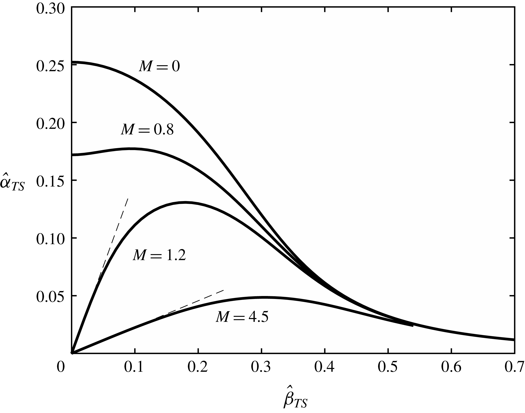
. The neutral curves for four different subsonic and supersonic Mach numbers are plotted in figure 2. The neutral curve can be extended to
 $\hat{\unicode[STIX]{x1D6FD}}_{TS}<0$
by symmetry.
Neutral curve of the T–S wave in the (
 $\hat{\unicode[STIX]{x1D6FC}}_{TS}$
,
 $\hat{\unicode[STIX]{x1D6FD}}_{TS}$
) plane for different Mach numbers. The dashed lines represent
 $\hat{\unicode[STIX]{x1D6FD}}_{TS}=\sqrt{M^{2}-1}\hat{\unicode[STIX]{x1D6FC}}_{TS}$
.

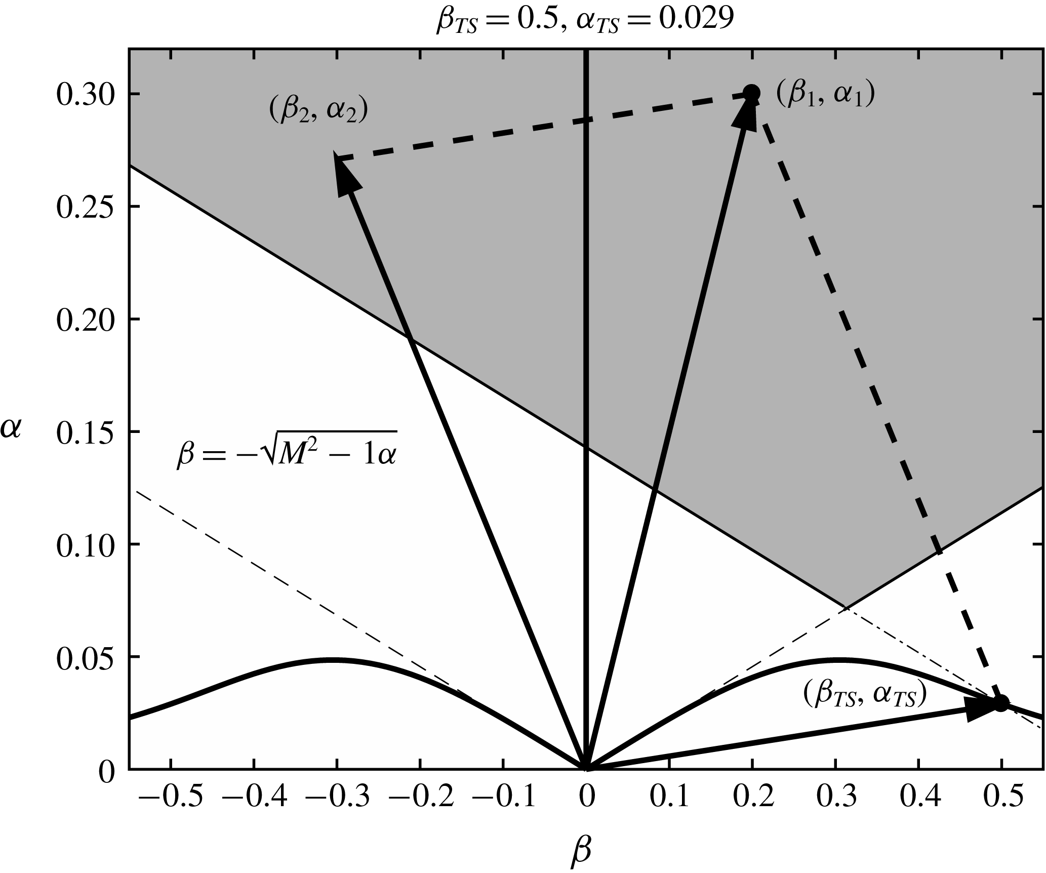
An illustration showing the selection of the sound waves which satisfy the resonance conditions (2.29) for a given T–S wave. The dash-dotted line represents
 $\hat{\unicode[STIX]{x1D6FD}}_{1}-\hat{\unicode[STIX]{x1D6FD}}_{TS}=-\sqrt{M^{2}-1}(\hat{\unicode[STIX]{x1D6FC}}_{1}-\hat{\unicode[STIX]{x1D6FC}}_{TS})$
.

A T–S mode can be excited by different combinations of two slow sound waves. A procedure for the choice of the sound waves is illustrated in figure 3 and described below.
(i) Choice of sound wave 1 (
 $\hat{\unicode[STIX]{x1D6FC}}_{1}$
,
$\hat{\unicode[STIX]{x1D6FD}}_{1}$
,
$\hat{\unicode[STIX]{x1D714}}_{1}$
). Its frequency can be arbitrary, but its wavenumbers must satisfy
$|\hat{\unicode[STIX]{x1D6FD}}_{1}|<\sqrt{M^{2}-1}\hat{\unicode[STIX]{x1D6FC}}_{1}$
.
(ii) Choice of sound wave 2 (
$\hat{\unicode[STIX]{x1D6FC}}_{2}$
,
$\hat{\unicode[STIX]{x1D6FD}}_{2}$
,
$\hat{\unicode[STIX]{x1D714}}_{2}$
). Its wavenumbers and frequency are determined from the resonance conditions (2.29). The wavenumbers must be in the region
$|\hat{\unicode[STIX]{x1D6FD}}_{2}|<\sqrt{M^{2}-1}\hat{\unicode[STIX]{x1D6FC}}_{2}$
too, this is, on recalling (2.29), (2.100)which together with$$\begin{eqnarray}\hat{\unicode[STIX]{x1D6FD}}_{1}-\hat{\unicode[STIX]{x1D6FD}}_{TS}>-\sqrt{M^{2}-1}(\hat{\unicode[STIX]{x1D6FC}}_{1}-\hat{\unicode[STIX]{x1D6FC}}_{TS}),\end{eqnarray}$$
$\hat{\unicode[STIX]{x1D6FD}}_{1}<\sqrt{M^{2}-1}\hat{\unicode[STIX]{x1D6FC}}_{1}$
(see (2.25)) represents the shaded region in figure 3. For any (
$\hat{\unicode[STIX]{x1D6FC}}_{1}$
,
$\hat{\unicode[STIX]{x1D6FD}}_{1}$
) in that region, it is always possible to find another sound wave to satisfy the resonance conditions, thereby exciting the T–S wave.










2.7.3 Forced response
At next order, the equations in the lower deck read
 $$\begin{eqnarray}\left.\begin{array}{@{}c@{}}\text{i}\hat{\unicode[STIX]{x1D6FC}}_{TS}\hat{U} _{2}+\hat{V}_{2,Y}+\text{i}\hat{\unicode[STIX]{x1D6FD}}_{TS}{\hat{W}}_{2}=-A^{\prime }(x_{1})\hat{u} _{TS},\\ \begin{array}{@{}rcl@{}}\text{i}(\hat{\unicode[STIX]{x1D6FC}}_{TS}\unicode[STIX]{x1D706}_{0}Y-\hat{\unicode[STIX]{x1D714}}_{TS})\hat{U} _{2}+\unicode[STIX]{x1D706}_{0}\hat{V}_{2}\, & =\, & -\text{i}\hat{\unicode[STIX]{x1D6FC}}_{TS}\hat{P}_{2}+\hat{U} _{2,YY}-\unicode[STIX]{x1D706}_{1}x_{1}A\hat{v}_{TS}\\ \, & \, & -\,\unicode[STIX]{x1D6EC}(x_{1})Y\hat{u} _{TS}-A^{\prime }(x_{1})\hat{p}_{TS}-N_{1},\end{array}\\ \text{i}(\hat{\unicode[STIX]{x1D6FC}}_{TS}\unicode[STIX]{x1D706}_{0}Y-\hat{\unicode[STIX]{x1D714}}_{TS}){\hat{W}}_{2}=-\text{i}\hat{\unicode[STIX]{x1D6FD}}_{TS}\hat{P}_{2}+{\hat{W}}_{2,YY}-\unicode[STIX]{x1D6EC}(x_{1})Y{\hat{w}}_{TS}-N_{3},\end{array}\right\}\end{eqnarray}$$
where
 $\unicode[STIX]{x1D6EC}$
is defined by
 $$\begin{eqnarray}\unicode[STIX]{x1D6EC}(x_{1})=\unicode[STIX]{x1D706}_{0}A^{\prime }(x_{1})+\text{i}\hat{\unicode[STIX]{x1D6FC}}_{TS}\unicode[STIX]{x1D706}_{1}x_{1}A,\end{eqnarray}$$
and the inhomogeneous terms
 $N_{1}$
and
 $N_{3}$
are given by
 $$\begin{eqnarray}\left.\begin{array}{@{}c@{}}N_{1}=\text{i}(\hat{\unicode[STIX]{x1D6FC}}_{1}-\hat{\unicode[STIX]{x1D6FC}}_{2})\hat{U} _{1}^{(1)}\hat{U} _{1}^{(2)\ast }+\text{i}\hat{\unicode[STIX]{x1D6FD}}_{1}{\hat{W}}_{1}^{(2)\ast }\hat{U} _{1}^{(1)}-\text{i}\hat{\unicode[STIX]{x1D6FD}}_{2}{\hat{W}}_{1}^{(1)}\hat{U} _{1}^{(2)\ast }+\hat{V}_{1}^{(1)}\hat{U} _{1Y}^{(2)\ast }+\hat{V}_{1}^{(2)\ast }\hat{U} _{1Y}^{(1)},\\ N_{3}=\text{i}\hat{\unicode[STIX]{x1D6FC}}_{1}{\hat{W}}_{1}^{(1)}\hat{U} _{1}^{(2)\ast }-\text{i}\hat{\unicode[STIX]{x1D6FC}}_{2}{\hat{W}}_{1}^{(2)\ast }\hat{U} _{1}^{(1)}+\text{i}(\hat{\unicode[STIX]{x1D6FD}}_{1}-\hat{\unicode[STIX]{x1D6FD}}_{2}){\hat{W}}_{1}^{(1)}{\hat{W}}_{1}^{(2)\ast }+\hat{V}_{1}^{(1)}{\hat{W}}_{1Y}^{(2)\ast }+\hat{V}_{1}^{(2)\ast }{\hat{W}}_{1Y}^{(1)}.\end{array}\right\}\end{eqnarray}$$
After rearranging (2.101) as we did before with (2.76), an inhomogeneous Airy equation for
 $\hat{V}_{2,YY}$
can be obtained,
 $$\begin{eqnarray}\left\{\frac{\unicode[STIX]{x2202}^{2}}{\unicode[STIX]{x2202}Y^{2}}-\text{i}(\hat{\unicode[STIX]{x1D6FC}}_{TS}\unicode[STIX]{x1D706}_{0}Y-\hat{\unicode[STIX]{x1D714}}_{TS})\right\}\hat{V}_{2,YY}=\unicode[STIX]{x1D6EC}Y\hat{V}_{TS,YY}-\text{i}(\hat{\unicode[STIX]{x1D6FC}}_{TS}N_{1}+\hat{\unicode[STIX]{x1D6FD}}_{TS}N_{3})_{Y}.\end{eqnarray}$$
The solution can be expressed as (cf. Wu (Reference Wu2001b ))
 $$\begin{eqnarray}\displaystyle \hat{V}_{2,Y} & = & \displaystyle {\textstyle \frac{1}{3}}(\text{i}\hat{\unicode[STIX]{x1D6FC}}_{TS}\unicode[STIX]{x1D706}_{0})^{-1}\unicode[STIX]{x1D6EC}(x_{1})\{(\tilde{\unicode[STIX]{x1D702}}-3\tilde{\unicode[STIX]{x1D702}}_{0})\text{Ai}(\tilde{\unicode[STIX]{x1D702}})+2\tilde{\unicode[STIX]{x1D702}}_{0}\text{Ai}(\tilde{\unicode[STIX]{x1D702}}_{0})\}\nonumber\\ \displaystyle & & \displaystyle +\,\int _{\tilde{\unicode[STIX]{x1D702}}_{0}}^{\tilde{\unicode[STIX]{x1D702}}}\tilde{M}(\unicode[STIX]{x1D702}^{\prime },\tilde{\unicode[STIX]{x1D702}}_{0})\,\text{d}\unicode[STIX]{x1D702}^{\prime }+q_{2}\int _{\tilde{\unicode[STIX]{x1D702}}_{0}}^{\tilde{\unicode[STIX]{x1D702}}}\text{Ai}(\unicode[STIX]{x1D702}^{\prime })\,\text{d}\unicode[STIX]{x1D702}^{\prime },\end{eqnarray}$$
where
 $q_{2}$
is a function of
 $x_{1}$
, and
 $\tilde{M}$
is given by
 $$\begin{eqnarray}\tilde{M}(\tilde{\unicode[STIX]{x1D702}},\tilde{\unicode[STIX]{x1D702}}_{0})=\unicode[STIX]{x03C0}\left\{\text{Bi}(\tilde{\unicode[STIX]{x1D702}})\int _{\infty }^{\tilde{\unicode[STIX]{x1D702}}}\text{Ai}(\unicode[STIX]{x1D702}^{\prime })H(Y^{\prime })\,\text{d}\unicode[STIX]{x1D702}^{\prime }-\text{Ai}(\tilde{\unicode[STIX]{x1D702}})\int _{\tilde{\unicode[STIX]{x1D702}}_{0}}^{\tilde{\unicode[STIX]{x1D702}}}\text{Bi}(\unicode[STIX]{x1D702}^{\prime })H(Y^{\prime })\,\text{d}\unicode[STIX]{x1D702}^{\prime }\right\},\end{eqnarray}$$
with
 $H=-(\hat{\unicode[STIX]{x1D6FC}}_{TS}\unicode[STIX]{x1D706}_{0})^{-1}[\hat{\unicode[STIX]{x1D6FC}}_{TS}N_{1}+\hat{\unicode[STIX]{x1D6FD}}_{TS}N_{3}]_{Y}$
, and
 $\text{Bi}$
being the Airy function.
At this order, the matching condition with the main-deck solution (2.67) reads
 $$\begin{eqnarray}\hat{V}_{2,Y}\rightarrow -\text{i}\hat{\unicode[STIX]{x1D6FC}}_{TS}\unicode[STIX]{x1D706}_{0}B_{2}-(\text{i}\hat{\unicode[STIX]{x1D6FC}}_{TS}\unicode[STIX]{x1D706}_{1}x_{1}A+\unicode[STIX]{x1D706}_{0}A^{\prime }(x_{1}))B_{1}\quad \text{as}~Y\rightarrow \infty ,\end{eqnarray}$$
and thus
 $$\begin{eqnarray}\displaystyle & & \displaystyle -\text{i}\hat{\unicode[STIX]{x1D6FC}}_{TS}\unicode[STIX]{x1D706}_{0}B_{2}-(\text{i}\hat{\unicode[STIX]{x1D6FC}}_{TS}\unicode[STIX]{x1D706}_{1}x_{1}A+\unicode[STIX]{x1D706}_{0}A^{\prime }(x_{1}))B_{1}={\textstyle \frac{2}{3}}(\text{i}\hat{\unicode[STIX]{x1D6FC}}_{TS}\unicode[STIX]{x1D706}_{0})^{-1}\unicode[STIX]{x1D6EC}\tilde{\unicode[STIX]{x1D702}}_{0}\text{Ai}(\tilde{\unicode[STIX]{x1D702}}_{0})\nonumber\\ \displaystyle & & \displaystyle \quad +\,\int _{\tilde{\unicode[STIX]{x1D702}}_{0}}^{\infty }\tilde{M}(\unicode[STIX]{x1D702}^{\prime },\tilde{\unicode[STIX]{x1D702}}_{0})\,\text{d}\unicode[STIX]{x1D702}^{\prime }+q_{2}\int _{\tilde{\unicode[STIX]{x1D702}}_{0}}^{\infty }\text{Ai}(\unicode[STIX]{x1D702}^{\prime })\,\text{d}\unicode[STIX]{x1D702}^{\prime }.\end{eqnarray}$$
The no-slip condition is
 $$\begin{eqnarray}\hat{V}_{2,YYY}=(\hat{\unicode[STIX]{x1D6FC}}_{TS}^{2}+\hat{\unicode[STIX]{x1D6FD}}_{TS}^{2})\hat{P}_{2}-2\text{i}\hat{\unicode[STIX]{x1D6FC}}_{TS}A^{\prime }(x_{1})\hat{P}_{TS}\quad \text{at}~Y=0,\end{eqnarray}$$
leading to
 $$\begin{eqnarray}\displaystyle & & \displaystyle {\textstyle \frac{2}{3}}(\text{i}\hat{\unicode[STIX]{x1D6FC}}_{TS}\unicode[STIX]{x1D706}_{0})^{-1/3}\unicode[STIX]{x1D6EC}\{\text{Ai}^{\prime }(\tilde{\unicode[STIX]{x1D702}}_{0})-\tilde{\unicode[STIX]{x1D702}}_{0}\text{Ai}^{\prime \prime }(\tilde{\unicode[STIX]{x1D702}}_{0})\}+(\text{i}\hat{\unicode[STIX]{x1D6FC}}_{TS}\unicode[STIX]{x1D706}_{0})^{2/3}\left\{\unicode[STIX]{x03C0}\text{Bi}^{\prime }(\tilde{\unicode[STIX]{x1D702}}_{0})\int _{\infty }^{\tilde{\unicode[STIX]{x1D702}}_{0}}\text{Ai}(\unicode[STIX]{x1D702}^{\prime })H(Y^{\prime })\,\text{d}\unicode[STIX]{x1D702}^{\prime }\right\}\nonumber\\ \displaystyle & & \displaystyle \quad +\,(\text{i}\hat{\unicode[STIX]{x1D6FC}}_{TS}\unicode[STIX]{x1D706}_{0})^{2/3}q_{2}\text{Ai}^{\prime }(\tilde{\unicode[STIX]{x1D702}}_{0})=(\hat{\unicode[STIX]{x1D6FC}}_{TS}^{2}+\hat{\unicode[STIX]{x1D6FD}}_{TS}^{2})\hat{P}_{2}-2\text{i}\hat{\unicode[STIX]{x1D6FC}}_{TS}A^{\prime }(x_{1})\hat{P}_{TS}.\end{eqnarray}$$
With
 $B_{1}$
and
 $\hat{P}_{TS}$
being determined from (2.95) and (2.96), the relations (2.108), (2.70) and (2.110) form a system of three equations for four unknowns:
 $q_{2}$
,
 $P_{2}$
,
 $B_{2}$
and
 $A(x_{1})$
. The elimination of
 $P_{2}$
and
 $B_{2}$
yields
 $$\begin{eqnarray}aA^{\prime }+b(\text{i}\hat{\unicode[STIX]{x1D6FC}}_{TS}\unicode[STIX]{x1D706}_{1}x_{1}/\unicode[STIX]{x1D706}_{0})A+(\hat{\unicode[STIX]{x1D6FC}}_{TS}^{2}+\hat{\unicode[STIX]{x1D6FD}}_{TS}^{2})^{-1}\unicode[STIX]{x1D6E5}(\unicode[STIX]{x1D706}_{0})q_{2}={\mathcal{F}},\end{eqnarray}$$
where
 $$\begin{eqnarray}\displaystyle a & = & \displaystyle \frac{2}{3}\tilde{\unicode[STIX]{x1D702}}_{0}\text{Ai}(\tilde{\unicode[STIX]{x1D702}}_{0})+\left(\frac{\hat{\unicode[STIX]{x1D6FD}}_{TS}^{2}}{\hat{\unicode[STIX]{x1D6FE}}_{TS}^{2}}+\frac{2\hat{\unicode[STIX]{x1D6FC}}_{TS}^{2}}{\hat{\unicode[STIX]{x1D6FC}}_{TS}^{2}+\hat{\unicode[STIX]{x1D6FD}}_{TS}^{2}}\right)\int _{\tilde{\unicode[STIX]{x1D702}}_{0}}^{\infty }\text{Ai}(\unicode[STIX]{x1D702}^{\prime })\,\text{d}\unicode[STIX]{x1D702}^{\prime }\nonumber\\ \displaystyle & & \displaystyle +\,\frac{2}{3}\frac{\hat{\unicode[STIX]{x1D6FE}}_{TS}(\text{i}\hat{\unicode[STIX]{x1D6FC}}_{TS}\unicode[STIX]{x1D706}_{0})^{5/3}}{\hat{\unicode[STIX]{x1D6FC}}_{TS}^{2}(\hat{\unicode[STIX]{x1D6FC}}_{TS}^{2}+\hat{\unicode[STIX]{x1D6FD}}_{TS}^{2})}\{\text{Ai}^{\prime }(\tilde{\unicode[STIX]{x1D702}}_{0})-\tilde{\unicode[STIX]{x1D702}}_{0}\text{Ai}^{\prime \prime }(\tilde{\unicode[STIX]{x1D702}}_{0})\},\qquad\end{eqnarray}$$
 $$\begin{eqnarray}\displaystyle & \displaystyle b=\frac{2}{3}\tilde{\unicode[STIX]{x1D702}}_{0}\text{Ai}(\tilde{\unicode[STIX]{x1D702}}_{0})-\int _{\tilde{\unicode[STIX]{x1D702}}_{0}}^{\infty }\text{Ai}(\unicode[STIX]{x1D702}^{\prime })\,\text{d}\unicode[STIX]{x1D702}^{\prime }+\frac{2}{3}\frac{\hat{\unicode[STIX]{x1D6FE}}_{TS}(\text{i}\hat{\unicode[STIX]{x1D6FC}}_{TS}\unicode[STIX]{x1D706}_{0})^{5/3}}{\hat{\unicode[STIX]{x1D6FC}}_{TS}^{2}(\hat{\unicode[STIX]{x1D6FC}}_{TS}^{2}+\hat{\unicode[STIX]{x1D6FD}}_{TS}^{2})}\{\text{Ai}^{\prime }(\tilde{\unicode[STIX]{x1D702}}_{0})-\tilde{\unicode[STIX]{x1D702}}_{0}\text{Ai}^{\prime \prime }(\tilde{\unicode[STIX]{x1D702}}_{0})\},\qquad & \displaystyle\end{eqnarray}$$
 $$\begin{eqnarray}\displaystyle & \displaystyle {\mathcal{F}}=\unicode[STIX]{x1D712}\int _{\infty }^{\tilde{\unicode[STIX]{x1D702}}_{0}}\text{Ai}(\unicode[STIX]{x1D702}^{\prime })H(Y^{\prime })\,\text{d}\unicode[STIX]{x1D702}^{\prime }-\text{i}\hat{\unicode[STIX]{x1D6FC}}_{TS}\int _{\tilde{\unicode[STIX]{x1D702}}_{0}}^{\infty }\tilde{M}(\unicode[STIX]{x1D702}^{\prime },\tilde{\unicode[STIX]{x1D702}}_{0})\,\text{d}\unicode[STIX]{x1D702}^{\prime },\qquad & \displaystyle\end{eqnarray}$$
 $$\begin{eqnarray}\displaystyle & \unicode[STIX]{x1D712}=\unicode[STIX]{x03C0}\unicode[STIX]{x1D706}_{0}\hat{\unicode[STIX]{x1D6FE}}_{TS}(\text{i}\hat{\unicode[STIX]{x1D6FC}}_{TS}\unicode[STIX]{x1D706}_{0})^{2/3}\text{Bi}^{\prime }(\tilde{\unicode[STIX]{x1D702}}_{0})/(\hat{\unicode[STIX]{x1D6FC}}_{TS}^{2}+\hat{\unicode[STIX]{x1D6FD}}_{TS}^{2}).\qquad & \displaystyle\end{eqnarray}$$
Since
 $\unicode[STIX]{x1D6E5}(\unicode[STIX]{x1D706}_{0})=0$
, we arrive at the evolution equation for
 $A(x_{1})$
,
 $$\begin{eqnarray}A^{\prime }(x_{1})=\unicode[STIX]{x1D70E}x_{1}A+N,\end{eqnarray}$$
where
 $$\begin{eqnarray}\unicode[STIX]{x1D70E}=-\text{i}\hat{\unicode[STIX]{x1D6FC}}_{TS}\unicode[STIX]{x1D706}_{1}b/(\unicode[STIX]{x1D706}_{0}a),\quad N={\mathcal{F}}/a.\end{eqnarray}$$
3 Receptivity: evolution from the forced response to eigenmode
3.1 Matching between T–S wave solution and upstream forced response
The amplitude equation (2.116) describes the evolution of the forced response upstream of the T–S wave (figure 4). On assuming that the amplitude of the T–S wave vanishes, i.e.
 $A(x_{1})\rightarrow 0$
as
 $x_{1}\rightarrow -\infty$
, the equation (2.116) has the solution (Wu Reference Wu1999)
 $$\begin{eqnarray}A(x_{1})=N\text{e}^{\unicode[STIX]{x1D70E}x_{1}^{2}/2}\int _{-\infty }^{x_{1}}\text{e}^{-\unicode[STIX]{x1D70E}\unicode[STIX]{x1D709}^{2}/2}\,\text{d}\unicode[STIX]{x1D709}.\end{eqnarray}$$
It can be shown that as
 $x_{1}\rightarrow -\infty$
,
 $$\begin{eqnarray}A(x_{1})\rightarrow \frac{N}{\unicode[STIX]{x1D70E}(-x_{1})}+O(x_{1}^{-3}).\end{eqnarray}$$
Receptivity mechanism due to sound–sound interaction.

To demonstrate the matching with the upstream response, we note that at an upstream position
 $x$
(figure 4),
 $q_{2}$
represents the amplitude of the forced response,
 $A_{F}$
,
 $$\begin{eqnarray}A_{F}\equiv q_{2}=\frac{\hat{\unicode[STIX]{x1D6FC}}_{TS}^{2}+\hat{\unicode[STIX]{x1D6FD}}_{TS}^{2}}{\unicode[STIX]{x1D6E5}(\unicode[STIX]{x1D706})}{\mathcal{F}}.\end{eqnarray}$$
By performing a Taylor expansion of
 $\unicode[STIX]{x1D6E5}(\unicode[STIX]{x1D706})$
about
 $\unicode[STIX]{x1D706}_{0}$
,
 $$\begin{eqnarray}\unicode[STIX]{x1D6E5}(\unicode[STIX]{x1D706})=\unicode[STIX]{x1D6E5}(\unicode[STIX]{x1D706}_{0})+\left.\frac{\unicode[STIX]{x2202}\unicode[STIX]{x1D6E5}}{\unicode[STIX]{x2202}\unicode[STIX]{x1D706}}\right|_{\unicode[STIX]{x1D706}_{0}}(\unicode[STIX]{x1D706}-\unicode[STIX]{x1D706}_{0})+\cdots =-\frac{\hat{\unicode[STIX]{x1D6FC}}_{TS}(\hat{\unicode[STIX]{x1D6FC}}_{TS}^{2}+\hat{\unicode[STIX]{x1D6FD}}_{TS}^{2})\unicode[STIX]{x1D706}_{0}b}{\text{i}\unicode[STIX]{x1D706}_{0}^{2}}(\unicode[STIX]{x1D706}-\unicode[STIX]{x1D706}_{0})+\cdots ,\end{eqnarray}$$
the behaviour of
 $A_{F}$
as
 $x\rightarrow x_{0}$
is obtained,
 $$\begin{eqnarray}A_{F}\rightarrow \frac{\unicode[STIX]{x1D706}_{0}{\mathcal{F}}}{\text{i}\hat{\unicode[STIX]{x1D6FC}}_{TS}b(\unicode[STIX]{x1D706}-\unicode[STIX]{x1D706}_{0})}.\end{eqnarray}$$
Substitution of (2.32) and (2.117) into (3.5) shows that
 $$\begin{eqnarray}A_{F}\rightarrow R^{3/16}\frac{N}{\unicode[STIX]{x1D70E}(-x_{1})},\end{eqnarray}$$
which confirms that
 $$\begin{eqnarray}R^{3/16}A(x_{1})\rightarrow A_{F}\quad \text{as}~x_{1}\rightarrow -\infty .\end{eqnarray}$$
In the downstream limit
 $x_{1}\rightarrow +\infty$
, it can be shown that
 $$\begin{eqnarray}A(x_{1})\rightarrow A_{\infty }\text{e}^{\unicode[STIX]{x1D70E}x_{1}^{2}/2},\end{eqnarray}$$
with
 $$\begin{eqnarray}A_{\infty }=N\int _{-\infty }^{+\infty }\text{e}^{-\unicode[STIX]{x1D70E}\unicode[STIX]{x1D709}^{2}/2}\,\text{d}\unicode[STIX]{x1D709}=N\sqrt{\frac{2\unicode[STIX]{x03C0}}{\unicode[STIX]{x1D70E}}}.\end{eqnarray}$$
Further downstream where
 $x_{1}=O(R^{3/16})$
, the T–S wave eventually acquires an
 $O(1)$
growth rate (figure 4), and evolves exponentially over the fast streamwise scale
 $\bar{x}$
. The amplitude takes the form (Wu Reference Wu1999, Reference Wu2001b
)
 $$\begin{eqnarray}A\text{e}^{\text{i}\hat{\unicode[STIX]{x1D6FC}}_{TS}\bar{x}}=A_{\infty }\exp \left\{\text{i}R^{3/8}\int _{x_{0}}^{x}\hat{\unicode[STIX]{x1D6FC}}_{TS}(x)\,\text{d}x\right\},\end{eqnarray}$$
which shows that the downstream development is equivalent to a free modal evolution with
 $A_{\infty }$
being the initial amplitude.
3.2 Coupling coefficients
A convenient representation of the magnitude of the T–S wave is the maximum value of its streamwise velocity, which can be directly measured in experiments, e.g. King & Breuer (Reference King and Breuer2002). Solving the spanwise momentum equation, we obtain the spanwise velocity
 $$\begin{eqnarray}{\hat{W}}_{TS}=\frac{\text{i}\hat{\unicode[STIX]{x1D6FD}}_{TS}\text{Ai}^{\prime }(\tilde{\unicode[STIX]{x1D702}}_{0})}{\hat{\unicode[STIX]{x1D6FC}}_{TS}^{2}+\hat{\unicode[STIX]{x1D6FD}}_{TS}^{2}}L(\tilde{\unicode[STIX]{x1D702}}),\end{eqnarray}$$
where
 $L(\tilde{\unicode[STIX]{x1D702}})$
is the solution to the equation
 $L^{\prime \prime }-\tilde{\unicode[STIX]{x1D702}}L=1$
satisfying the boundary conditions
 $L(\tilde{\unicode[STIX]{x1D702}}_{0})=0$
and
 $L(\infty )=0$
. From the continuity equation, (2.93) and (2.72), it follows that the streamwise velocity at the neutral point is given by
 $$\begin{eqnarray}u_{TS}=\unicode[STIX]{x1D700}_{s}^{2}\bar{\unicode[STIX]{x1D700}}^{-1}R^{3/8}C^{1/8}\unicode[STIX]{x1D70F}_{w}^{1/2}\hat{\unicode[STIX]{x1D6FC}}_{TS}^{-1}A_{\infty }U_{m},\end{eqnarray}$$
where
 $$\begin{eqnarray}U_{m}=\max _{\tilde{\unicode[STIX]{x1D702}}}\left|\int _{\tilde{\unicode[STIX]{x1D702}}_{0}}^{\tilde{\unicode[STIX]{x1D702}}}\text{Ai}(\unicode[STIX]{x1D702}^{\prime })\,\text{d}\unicode[STIX]{x1D702}^{\prime }-\frac{\unicode[STIX]{x1D6FD}_{N}^{2}}{\unicode[STIX]{x1D6FC}_{N}^{2}+\unicode[STIX]{x1D6FD}_{N}^{2}}\text{Ai}^{\prime }(\tilde{\unicode[STIX]{x1D702}}_{0})L(\tilde{\unicode[STIX]{x1D702}})\right|.\end{eqnarray}$$
The coupling coefficient for the sound–sound interaction can be defined as
 $$\begin{eqnarray}C_{A}\equiv u_{TS}/\unicode[STIX]{x1D700}_{s}=\unicode[STIX]{x1D700}_{s}R^{9/16}C^{-1/16}\unicode[STIX]{x1D70F}_{w}^{-1/4}\hat{\unicode[STIX]{x1D6FC}}_{TS}^{-1}A_{\infty }U_{m}\equiv \unicode[STIX]{x1D700}_{s}R^{9/16}\unicode[STIX]{x1D6EC}_{SS}.\end{eqnarray}$$
Clearly,
 $\unicode[STIX]{x1D6EC}_{SS}$
is the rescaled coupling coefficient, and depends on the parameters such as
 $\hat{\unicode[STIX]{x1D714}}_{1}$
,
 ${\hat{c}}_{1}$
, etc.
4 Receptivity to slow acoustic waves interacting with distributed roughness
In this section, we consider the generation of T–S waves due to a sound wave interacting with distributed roughness. This receptivity mechanism has been studied previously for incompressible boundary layers (e.g. Choudhari (Reference Choudhari1993), Wu (Reference Wu2001b
)) and compressible boundary layers (Fedorov Reference Fedorov2003a
). The frequency of the sound wave is taken to be
 $O(R^{2/8})$
, comparable with that of the T–S wave. Earlier studies assumed that its phase speed was of
 $O(1)$
so that the wavenumber is
 $O(R^{2/8})$
; in the incompressible limit, the phase speed and wavenumber are infinite and zero, respectively. In this paper, the sound wave is taken to have a much smaller speed
 $c=O(R^{-1/8})$
so that its wavenumber is
 $O(R^{3/8})$
. Although the frequency and wavenumbers of such sound waves are comparable with those of T–S waves, the former does not excite the latter directly because they have different dispersion relations. A scale tuning mechanism is still required in order to satisfy the required resonance conditions. This can be provided by suitable distributed surface roughness. Sound waves on the triple-deck scale will lead to stronger receptivity.
4.1 Physical idea and asymptotic scaling
Sketch of the ‘difference-mode’ interaction between a sound wave and a wavy wall (distributed roughness) in the supersonic regime, featuring Mach wave radiation.

Suppose that a three-dimensional sound wave,
 $\unicode[STIX]{x1D700}_{s}\{\text{e}^{\text{i}(\hat{\unicode[STIX]{x1D6FC}}_{s}\bar{x}+\hat{\unicode[STIX]{x1D6FD}}_{s}\bar{z}+\hat{\unicode[STIX]{x1D6FE}}_{s}\bar{y}-\hat{\unicode[STIX]{x1D714}}_{s}\bar{t})}+\text{c.c.}\}$
, impinges on the boundary layer and, that a distributed roughness is present (figure 5), represented by a wavy wall, whose position is given by
 $$\begin{eqnarray}Y=h\hat{F}_{w}\{\text{e}^{\text{i}(\hat{\unicode[STIX]{x1D6FC}}_{w}\bar{x}+\hat{\unicode[STIX]{x1D6FD}}_{w}\bar{z}+\hat{\unicode[STIX]{x1D6FE}}_{w}\bar{y})}+\text{c.c.}\},\end{eqnarray}$$
where
 $h\ll 1$
is a measure of the roughness height, which is related to the physical height
 $h^{\ast }$
by the equation
 $$\begin{eqnarray}h=R^{5/8}C^{-5/8}\unicode[STIX]{x1D70F}_{w}^{-3/2}h^{\ast }/L.\end{eqnarray}$$
In (4.1),
 $\hat{F}_{w}$
is of
 $O(1)$
and can be set to unity, but is retained for book-keeping purpose. With the same scaling (2.28) for the wavenumbers as in the previous problem, the resonance conditions for the present mechanism are,
 $$\begin{eqnarray}\hat{\unicode[STIX]{x1D6FC}}_{s}-\hat{\unicode[STIX]{x1D6FC}}_{w}=\hat{\unicode[STIX]{x1D6FC}}_{TS},\quad \hat{\unicode[STIX]{x1D6FD}}_{s}-\hat{\unicode[STIX]{x1D6FD}}_{w}=\hat{\unicode[STIX]{x1D6FD}}_{TS},\quad \hat{\unicode[STIX]{x1D714}}_{s}=\hat{\unicode[STIX]{x1D714}}_{TS},\end{eqnarray}$$
which ensure that the difference mode produced through the interaction excites the T–S mode. It is interesting to note that in this case, the sum mode may excite T–S modes as well because one of the interacting elements, the roughness, is not subject to the restriction
 $\hat{\unicode[STIX]{x1D6FD}}_{w}<\sqrt{M^{2}-1}\hat{\unicode[STIX]{x1D6FC}}_{w}$
. The corresponding resonance conditions to meet would be
 $$\begin{eqnarray}\hat{\unicode[STIX]{x1D6FC}}_{s}+\hat{\unicode[STIX]{x1D6FC}}_{w}=\hat{\unicode[STIX]{x1D6FC}}_{TS},\quad \hat{\unicode[STIX]{x1D6FD}}_{s}+\hat{\unicode[STIX]{x1D6FD}}_{w}=\hat{\unicode[STIX]{x1D6FD}}_{TS},\quad \hat{\unicode[STIX]{x1D714}}_{s}=\hat{\unicode[STIX]{x1D714}}_{TS}.\end{eqnarray}$$
For the present mechanism, the solutions for the sound wave and the T–S eigenmode are the same as in the sound–sound interaction. Throughout § 5, we will thus consider only the solution for the roughness-induced mean-flow distortion and its interaction with the sound wave.
4.2 Upper deck
As in the previous problem, the wall-normal variable is
 $\bar{y}=R^{-1/8}C^{-3/8}\unicode[STIX]{x1D70F}_{w}^{-3/2}y$
, but the expansions become
 $$\begin{eqnarray}\displaystyle & \tilde{\boldsymbol{u}}=\unicode[STIX]{x1D700}_{s}\boldsymbol{u}_{s}+hR^{-2/8}\boldsymbol{u}_{M}+\unicode[STIX]{x1D700}_{s}h\bar{\unicode[STIX]{x1D700}}^{-1}(\boldsymbol{u}_{TS}E_{TS}+\text{c.c.})+\unicode[STIX]{x1D700}_{s}h\boldsymbol{u}_{2}+\cdots , & \displaystyle\end{eqnarray}$$
 $$\begin{eqnarray}\displaystyle & \tilde{p}=\unicode[STIX]{x1D700}_{s}p_{s}+hR^{-2/8}p_{M}+\unicode[STIX]{x1D700}_{s}h\bar{\unicode[STIX]{x1D700}}^{-1}(p_{TS}E_{TS}+\text{c.c.})+\unicode[STIX]{x1D700}_{s}hp_{2}+\cdots , & \displaystyle\end{eqnarray}$$
 $$\begin{eqnarray}\displaystyle & \tilde{\unicode[STIX]{x1D70C}}=\unicode[STIX]{x1D700}_{s}R_{s}+hR^{-2/8}R_{M}+\unicode[STIX]{x1D700}_{s}h\bar{\unicode[STIX]{x1D700}}^{-1}(R_{TS}E_{TS}+\text{c.c.})+\unicode[STIX]{x1D700}_{s}hR_{2}+\cdots , & \displaystyle\end{eqnarray}$$
 $$\begin{eqnarray}\displaystyle & \tilde{\unicode[STIX]{x1D70F}}=\unicode[STIX]{x1D700}_{s}\unicode[STIX]{x1D70F}_{s}+hR^{-2/8}\unicode[STIX]{x1D70F}_{M}+\unicode[STIX]{x1D700}_{s}h\bar{\unicode[STIX]{x1D700}}^{-1}(\unicode[STIX]{x1D70F}_{TS}E_{TS}+\text{c.c.})+\unicode[STIX]{x1D700}_{s}h\unicode[STIX]{x1D70F}_{2}+\cdots . & \displaystyle\end{eqnarray}$$
Substitution of (4.5)–(4.8) into (2.2)–(2.6) yields, at order
 $O(\unicode[STIX]{x1D700}_{s})$
, the same linearized equations for the sound wave as in the previous problem, and at
 $O(hR^{-2/8})$
, the equations for the roughness-induced mean-flow distortion. The solution for the latter is now considered. The general expression for the pressure is
 $$\begin{eqnarray}p_{M}=P_{M}(r^{+}\text{e}^{\text{i}\hat{\unicode[STIX]{x1D6FE}}_{w}\bar{y}}+r^{-}\text{e}^{-\text{i}\hat{\unicode[STIX]{x1D6FE}}_{w}\bar{y}})E_{w}\quad \text{with}~E_{w}=\text{e}^{\text{i}(\hat{\unicode[STIX]{x1D6FC}}_{w}\bar{x}+\hat{\unicode[STIX]{x1D6FD}}_{w}\bar{z})},\end{eqnarray}$$
where
 $\hat{\unicode[STIX]{x1D6FE}}_{w}=\sqrt{(M^{2}-1)\hat{\unicode[STIX]{x1D6FC}}_{w}^{2}-\hat{\unicode[STIX]{x1D6FD}}_{w}^{2}}$
, and
 $r^{\pm }$
are constants. Two cases have to be distinguished, depending on whether
 $\sqrt{M^{2}-1}\hat{\unicode[STIX]{x1D6FC}}_{w}-\hat{\unicode[STIX]{x1D6FD}}_{w}$
is positive or negative. For the former case, two families of straight lines,
 $$\begin{eqnarray}\hat{\unicode[STIX]{x1D6FC}}_{w}\bar{x}\pm \sqrt{(M^{2}-1)\hat{\unicode[STIX]{x1D6FC}}_{w}^{2}-\hat{\unicode[STIX]{x1D6FD}}_{w}^{2}}\bar{y}=\text{const.},\end{eqnarray}$$
represent the fronts of the so-called Mach waves. We need to make use of the principle of causality, or equivalently, the requirement that the vertical group velocity is positive,
 $\unicode[STIX]{x2202}\hat{\unicode[STIX]{x1D714}}_{w}/\unicode[STIX]{x2202}\hat{\unicode[STIX]{x1D6FE}}_{w}>0$
, in order to choose the correct branch for the outgoing wave. By using the dispersion relation
 $-M^{2}(\hat{\unicode[STIX]{x1D6FC}}_{w}-\hat{\unicode[STIX]{x1D714}}_{w})^{2}+\hat{\unicode[STIX]{x1D6FC}}_{w}^{2}+\hat{\unicode[STIX]{x1D6FD}}_{w}^{2}+\hat{\unicode[STIX]{x1D6FE}}_{w}^{2}=0$
and differentiating with respect to
 $\hat{\unicode[STIX]{x1D6FE}}_{w}$
, it follows that
 $$\begin{eqnarray}\frac{\unicode[STIX]{x2202}\hat{\unicode[STIX]{x1D714}}_{w}}{\unicode[STIX]{x2202}\hat{\unicode[STIX]{x1D6FE}}_{w}}=-\!\left.\frac{\hat{\unicode[STIX]{x1D6FE}}_{w}}{M^{2}(\hat{\unicode[STIX]{x1D6FC}}_{w}-\hat{\unicode[STIX]{x1D714}}_{w})}\right|_{\hat{\unicode[STIX]{x1D714}}_{w}\rightarrow 0}>0,\end{eqnarray}$$
which is possible only if
 $\hat{\unicode[STIX]{x1D6FE}}_{w}<0$
. Thus, the outgoing wave is
 $\text{e}^{-\text{i}\hat{\unicode[STIX]{x1D6FE}}_{w}\bar{y}}$
and the correct branch is
 $\text{e}^{-\text{i}\sqrt{(M^{2}-1)\hat{\unicode[STIX]{x1D6FC}}_{w}^{2}-\hat{\unicode[STIX]{x1D6FD}}_{w}^{2}}\bar{y}}$
(see figure 5); we set
 $r^{+}=0$
and
 $r^{-}=1$
in (4.9) on the understanding that
 $r^{-}$
can be absorbed into
 $P_{M}$
. On the other hand, if
 $\hat{\unicode[STIX]{x1D6FD}}_{w}>\sqrt{M^{2}-1}\hat{\unicode[STIX]{x1D6FC}}_{w}$
, the other branch
 $\text{e}^{\text{i}\sqrt{(M^{2}-1)\hat{\unicode[STIX]{x1D6FC}}_{w}^{2}-\hat{\unicode[STIX]{x1D6FD}}_{w}^{2}}\bar{y}}$
, with
 $r^{+}=1$
and
 $r^{-}=0$
, needs to be chosen to ensure that
 $p_{M}\sim \text{e}^{-\unicode[STIX]{x1D708}\bar{y}}$
with
 $\unicode[STIX]{x1D708}=\sqrt{\hat{\unicode[STIX]{x1D6FD}}_{w}^{2}-(M^{2}-1)\hat{\unicode[STIX]{x1D6FC}}_{w}^{2}}$
being a real number. In this case, the roughness-induced perturbation is trapped within the boundary layer.
At next orders, equations similar to those for the sound–sound interaction hold:
 $O(\unicode[STIX]{x1D700}_{s}hR^{3/16})$
for the T–S wave and
 $O(\unicode[STIX]{x1D700}_{s}h)$
for the response. It turns out that, in order for the sum mode to generate a T–S wave, the wavenumbers must satisfy
 $\hat{\unicode[STIX]{x1D6FD}}_{w}>\sqrt{M^{2}-1}\hat{\unicode[STIX]{x1D6FC}}_{w}$
, while for the difference mode to generate a T–S wave
 $\hat{\unicode[STIX]{x1D6FD}}_{w}<\sqrt{M^{2}-1}\hat{\unicode[STIX]{x1D6FC}}_{w}$
instead.
4.3 Main deck
The transverse variable is
 ${\tilde{y}}=C^{-1/2}\unicode[STIX]{x1D70F}_{w}^{-1}y=O(1)$
, and the expansions take the form
 $$\begin{eqnarray}\displaystyle & \tilde{u} =C^{1/8}\unicode[STIX]{x1D70F}_{w}^{1/2}[\unicode[STIX]{x1D700}_{s}R^{1/8}\hat{u} _{s}+hR^{-1/8}\hat{u} _{M}E_{w}+\unicode[STIX]{x1D700}_{s}h\bar{\unicode[STIX]{x1D700}}^{-1}R^{1/8}\tilde{u} _{TS}+\unicode[STIX]{x1D700}_{s}hR^{1/8}\hat{u} _{2}E_{TS}+\cdots ],\qquad & \displaystyle\end{eqnarray}$$
 $$\begin{eqnarray}\displaystyle & \tilde{v}=C^{1/4}[\unicode[STIX]{x1D700}_{s}\hat{v}_{s}+hR^{-2/8}\hat{v}_{M}E_{w}+\unicode[STIX]{x1D700}_{s}^{2}\bar{\unicode[STIX]{x1D700}}^{-1}\tilde{v}_{TS}+\unicode[STIX]{x1D700}_{s}h\hat{v}_{2}E_{TS}+\cdots ],\qquad & \displaystyle\end{eqnarray}$$
 $$\begin{eqnarray}\displaystyle & \tilde{w}=C^{1/4}\unicode[STIX]{x1D70F}_{w}[\unicode[STIX]{x1D700}_{s}{\hat{w}}_{s}+hR^{-2/8}{\hat{w}}_{M}E_{w}+\unicode[STIX]{x1D700}_{s}h\bar{\unicode[STIX]{x1D700}}^{-1}\tilde{w}_{TS}+\unicode[STIX]{x1D700}_{s}h{\hat{w}}_{2}E_{TS}+\cdots ],\qquad & \displaystyle\end{eqnarray}$$
 $$\begin{eqnarray}\displaystyle & \tilde{p}=C^{1/4}[\unicode[STIX]{x1D700}_{s}\hat{p}_{s}+hR^{-2/8}\hat{p}_{M}E_{w}+\unicode[STIX]{x1D700}_{s}h\bar{\unicode[STIX]{x1D700}}^{-1}\tilde{p}_{TS}+\unicode[STIX]{x1D700}_{s}h\hat{p}_{2}E_{TS}+\cdots ],\qquad & \displaystyle\end{eqnarray}$$
 $$\begin{eqnarray}\displaystyle & \tilde{\unicode[STIX]{x1D70C}}=C^{1/8}\unicode[STIX]{x1D70F}_{w}^{1/2}[\unicode[STIX]{x1D700}_{s}R^{1/8}\hat{R}_{s}+hR^{-1/8}\hat{R}_{M}E_{w}+\unicode[STIX]{x1D700}_{s}h\bar{\unicode[STIX]{x1D700}}^{-1}R^{1/8}\tilde{R}_{TS}+\unicode[STIX]{x1D700}_{s}hR^{1/8}\hat{R}_{2}E_{TS}+\cdots ],\qquad & \displaystyle\end{eqnarray}$$
 $$\begin{eqnarray}\displaystyle & \tilde{\unicode[STIX]{x1D70F}}=C^{1/8}\unicode[STIX]{x1D70F}_{w}^{1/2}[\unicode[STIX]{x1D700}_{s}R^{1/8}\hat{\unicode[STIX]{x1D70F}}_{s}+h\hat{\unicode[STIX]{x1D70F}}_{M}E_{w}+\unicode[STIX]{x1D700}_{s}h\bar{\unicode[STIX]{x1D700}}^{-1}R^{2/8}\tilde{\unicode[STIX]{x1D70F}}_{TS}+\unicode[STIX]{x1D700}_{s}hR^{2/8}\hat{\unicode[STIX]{x1D70F}}_{2}E_{TS}+\cdots ].\qquad & \displaystyle\end{eqnarray}$$
The solution for the mean-flow distortion is (Smith, Sykes & Brighton Reference Smith, Sykes and Brighton1977)
 $$\begin{eqnarray}\hat{u} _{M}=\hat{A}_{M}U_{B}^{\prime },\quad \hat{v}_{M}=-\text{i}\unicode[STIX]{x1D6FC}_{w}\hat{A}_{M}U_{B},\end{eqnarray}$$
where
 $\hat{A}_{M}$
is a constant.
4.4 Lower deck
The expansions take the form
 $$\begin{eqnarray}\displaystyle & \tilde{u} =C^{1/8}\unicode[STIX]{x1D70F}_{w}^{1/2}[\unicode[STIX]{x1D700}_{s}R^{1/8}\hat{U} _{s}+hR^{-1/8}\hat{U} _{M}E_{w}+\unicode[STIX]{x1D700}_{s}hR^{1/8}(\bar{\unicode[STIX]{x1D700}}^{-1}A(x_{1})\hat{U} _{TS}+\hat{U} _{2})E_{TS}+\cdots ],\qquad & \displaystyle\end{eqnarray}$$
 $$\begin{eqnarray}\displaystyle & \tilde{v}=C^{3/8}\unicode[STIX]{x1D70F}_{w}^{1/2}[\unicode[STIX]{x1D700}_{s}R^{-1/8}\hat{V}_{s}+hR^{-3/8}\hat{V}_{M}E_{w}+\unicode[STIX]{x1D700}_{s}hR^{-1/8}(\bar{\unicode[STIX]{x1D700}}^{-1}A(x_{1})\hat{V}_{TS}+\hat{V}_{2})E_{TS}+\cdots ],\qquad & \displaystyle\end{eqnarray}$$
 $$\begin{eqnarray}\displaystyle & \tilde{w}=C^{1/8}\unicode[STIX]{x1D70F}_{w}^{1/2}[\unicode[STIX]{x1D700}_{s}R^{1/8}{\hat{W}}_{s}+hR^{-1/8}{\hat{W}}_{M}E_{w}+\unicode[STIX]{x1D700}_{s}hR^{1/8}(\bar{\unicode[STIX]{x1D700}}^{-1}A(x_{1}){\hat{W}}_{TS}+{\hat{W}}_{2})E_{TS}+\cdots ],\qquad & \displaystyle\end{eqnarray}$$
 $$\begin{eqnarray}\displaystyle & \tilde{p}=C^{1/4}[\unicode[STIX]{x1D700}_{s}\hat{P}_{s}+hR^{-1/4}\hat{P}_{M}E_{w}+\unicode[STIX]{x1D700}_{s}h(\bar{\unicode[STIX]{x1D700}}^{-1}A(x_{1})\hat{P}_{TS}+\hat{P}_{2})E_{TS}+\cdots ].\qquad & \displaystyle\end{eqnarray}$$
The expansions for the density and temperature are omitted again since they play no role at leading order. The solution for the roughness-induced mean-flow distortion is given in appendix A.
4.4.1 Forced response
We now consider the forced response, which satisfies the same equations (2.101) for the interaction between two slow sound waves, except that the inhomogeneous terms
 $N_{1}$
and
 $N_{3}$
now read
 $$\begin{eqnarray}\left.\begin{array}{@{}c@{}}N_{1}=\text{i}(\hat{\unicode[STIX]{x1D6FC}}_{s}-\hat{\unicode[STIX]{x1D6FC}}_{w})\hat{U} _{s}\hat{U} _{M}^{\ast }+\text{i}\hat{\unicode[STIX]{x1D6FD}}_{s}{\hat{W}}_{M}^{\ast }\hat{U} _{s}-\text{i}\hat{\unicode[STIX]{x1D6FD}}_{w}{\hat{W}}_{s}\hat{U} _{M}^{\ast }+\hat{V}_{s}\hat{U} _{MY}^{\ast }+\hat{V}_{M}^{\ast }\hat{U} _{sY},\\ N_{3}=\text{i}\hat{\unicode[STIX]{x1D6FC}}_{s}{\hat{W}}_{s}\hat{U} _{M}^{\ast }-\text{i}\hat{\unicode[STIX]{x1D6FC}}_{w}{\hat{W}}_{M}^{\ast }\hat{U} _{s}+\text{i}(\hat{\unicode[STIX]{x1D6FD}}_{s}-\hat{\unicode[STIX]{x1D6FD}}_{w}){\hat{W}}_{s}{\hat{W}}_{M}^{\ast }+\hat{V}_{s}{\hat{W}}_{MY}^{\ast }+\hat{V}_{M}^{\ast }{\hat{W}}_{sY},\end{array}\right\}\end{eqnarray}$$
for the excitation by the difference mode. The forcing terms for the sum mode are
 $$\begin{eqnarray}\left.\begin{array}{@{}c@{}}N_{1}=\text{i}(\hat{\unicode[STIX]{x1D6FC}}_{s}+\hat{\unicode[STIX]{x1D6FC}}_{w})\hat{U} _{s}\hat{U} _{M}+\text{i}\hat{\unicode[STIX]{x1D6FD}}_{s}{\hat{W}}_{M}\hat{U} _{s}+\text{i}\hat{\unicode[STIX]{x1D6FD}}_{w}{\hat{W}}_{s}\hat{U} _{M}+\hat{V}_{s}\hat{U} _{MY}+\hat{V}_{M}\hat{U} _{sY},\\ N_{3}=\text{i}\hat{\unicode[STIX]{x1D6FC}}_{s}{\hat{W}}_{s}\hat{U} _{M}+\text{i}\hat{\unicode[STIX]{x1D6FC}}_{w}{\hat{W}}_{M}\hat{U} _{s}+\text{i}(\hat{\unicode[STIX]{x1D6FD}}_{s}+\hat{\unicode[STIX]{x1D6FD}}_{w}){\hat{W}}_{s}{\hat{W}}_{M}+\hat{V}_{s}{\hat{W}}_{MY}+\hat{V}_{M}{\hat{W}}_{sY}.\end{array}\right\}\end{eqnarray}$$
Note that the transverse velocity
 $\hat{V}_{s}$
of the acoustic-induced fluctuation contributes to the forcing for a sound wave on the triple-deck scale.
The boundary conditions for the forced response, for both difference- and sum-mode cases, read
 $$\begin{eqnarray}\hat{U} _{2}(0)=-(\text{i}\hat{\unicode[STIX]{x1D6FC}}_{s}\unicode[STIX]{x1D706}_{0})^{1/3}{\hat{U} _{s}}^{\prime }(\unicode[STIX]{x1D702}_{0})\hat{F}_{w},\quad \hat{V}_{2}(0)=0,\quad {\hat{W}}_{2}(0)=-(\text{i}\hat{\unicode[STIX]{x1D6FC}}_{s}\unicode[STIX]{x1D706}_{0})^{1/3}{{\hat{W}}_{s}}^{\prime }(\unicode[STIX]{x1D702}_{0})\hat{F}_{w},\end{eqnarray}$$
which implies that
 $\hat{V}_{2,Y}(0)=\text{i}(\text{i}\hat{\unicode[STIX]{x1D6FC}}_{s}\unicode[STIX]{x1D706}_{0})^{1/3}\{\hat{\unicode[STIX]{x1D6FC}}_{TS}{\hat{U} _{s}}^{\prime }(\unicode[STIX]{x1D702}_{0})+\hat{\unicode[STIX]{x1D6FD}}_{TS}{\hat{W}}_{s}^{\prime }(\unicode[STIX]{x1D702}_{0})\}\hat{F}_{w}$
, with the expressions for
 $\hat{U} _{s}^{\prime }(\unicode[STIX]{x1D702}_{0})$
and
 ${\hat{W}}_{s}^{\prime }(\unicode[STIX]{x1D702}_{0})$
being deduced from (2.91) and (2.89), respectively, as
 $$\begin{eqnarray}\displaystyle & \displaystyle \hat{U} _{s}^{\prime }(\unicode[STIX]{x1D702}_{0})=\frac{\text{i}\hat{P}_{s}}{\hat{\unicode[STIX]{x1D6FC}}_{s}(\text{i}\hat{\unicode[STIX]{x1D6FC}}_{s}\unicode[STIX]{x1D706}_{0})^{2/3}}\left[\frac{(\hat{\unicode[STIX]{x1D6FC}}_{s}^{2}+\hat{\unicode[STIX]{x1D6FD}}_{s}^{2})\text{Ai}(\unicode[STIX]{x1D702}_{0})}{\text{Ai}^{\prime }(\unicode[STIX]{x1D702}_{0})}-\hat{\unicode[STIX]{x1D6FD}}_{s}^{2}\int _{\unicode[STIX]{x1D702}_{0}}^{\infty }\text{Ai}(\tilde{\unicode[STIX]{x1D702}})\,\text{d}\tilde{\unicode[STIX]{x1D702}}\right], & \displaystyle\end{eqnarray}$$
 $$\begin{eqnarray}\displaystyle & \displaystyle {\hat{W}}_{s}^{\prime }(\unicode[STIX]{x1D702}_{0})=-\hat{\unicode[STIX]{x1D6FD}}_{s}\hat{P}_{s}\int _{\unicode[STIX]{x1D702}_{0}}^{\infty }\text{Ai}(\tilde{\unicode[STIX]{x1D702}})\,\text{d}\tilde{\unicode[STIX]{x1D702}}. & \displaystyle\end{eqnarray}$$
Rearranging the forced-response equations in the same way as we did for (2.101), it can be shown that the no-slip condition (4.25) implies that
 $$\begin{eqnarray}\displaystyle \hat{V}_{2,YYY} & = & \displaystyle (\hat{\unicode[STIX]{x1D6FC}}_{TS}^{2}+\hat{\unicode[STIX]{x1D6FD}}_{TS}^{2})\hat{P}_{2}-2\text{i}\hat{\unicode[STIX]{x1D6FC}}_{TS}A^{\prime }(x_{1})\hat{P}_{TS}\nonumber\\ \displaystyle & & \displaystyle +\,\hat{\unicode[STIX]{x1D714}}_{TS}(\text{i}\hat{\unicode[STIX]{x1D6FC}}_{s}\unicode[STIX]{x1D706}_{0})^{1/3}\{\hat{\unicode[STIX]{x1D6FC}}_{TS}{\hat{U} _{s}}^{\prime }(\unicode[STIX]{x1D702}_{0})+\hat{\unicode[STIX]{x1D6FD}}_{TS}{\hat{W}}_{s}^{\prime }(\unicode[STIX]{x1D702}_{0})\}\hat{F}_{w}\quad \text{at}~Y=0.\end{eqnarray}$$
An inhomogeneous Airy equation (2.104) for
 $\hat{V}_{2,YY}$
is obtained and solved to give
 $$\begin{eqnarray}\displaystyle \hat{V}_{2,Y} & = & \displaystyle {\textstyle \frac{1}{3}}(\text{i}\hat{\unicode[STIX]{x1D6FC}}_{TS}\unicode[STIX]{x1D706}_{0})^{-1}\unicode[STIX]{x1D6EC}(x_{1})\{(\tilde{\unicode[STIX]{x1D702}}-3\tilde{\unicode[STIX]{x1D702}}_{0})\text{Ai}(\tilde{\unicode[STIX]{x1D702}})+2\tilde{\unicode[STIX]{x1D702}}_{0}\text{Ai}(\tilde{\unicode[STIX]{x1D702}}_{0})\}+\int _{\tilde{\unicode[STIX]{x1D702}}_{0}}^{\tilde{\unicode[STIX]{x1D702}}}\tilde{M}(\unicode[STIX]{x1D702}^{\prime },\tilde{\unicode[STIX]{x1D702}}_{0})\,\text{d}\unicode[STIX]{x1D702}^{\prime }\nonumber\\ \displaystyle & & \displaystyle +\,q_{2}\int _{\tilde{\unicode[STIX]{x1D702}}_{0}}^{\tilde{\unicode[STIX]{x1D702}}}\text{Ai}(\unicode[STIX]{x1D702}^{\prime })\,\text{d}\unicode[STIX]{x1D702}^{\prime }+\text{i}(\text{i}\hat{\unicode[STIX]{x1D6FC}}_{s}\unicode[STIX]{x1D706}_{0})^{1/3}\{\hat{\unicode[STIX]{x1D6FC}}_{TS}{\hat{U} _{s}}^{\prime }(\unicode[STIX]{x1D702}_{0})+\hat{\unicode[STIX]{x1D6FD}}_{TS}{\hat{W}}_{s}^{\prime }(\unicode[STIX]{x1D702}_{0})\}\hat{F}_{w},\end{eqnarray}$$
where
 $q_{2}$
is a function of
 $x_{1}$
, and
 $\tilde{M}$
has the same expression as (2.106) but with
 $H$
being replaced by the forcing (4.23) or (4.24) pertaining to the present problem.
The matching condition with the main-deck solution (2.67) gives (2.107), but with the solution (4.29) it leads to
 $$\begin{eqnarray}\displaystyle & & \displaystyle -\text{i}\hat{\unicode[STIX]{x1D6FC}}_{TS}\unicode[STIX]{x1D706}_{0}\hat{B}_{2}-(\text{i}\hat{\unicode[STIX]{x1D6FC}}_{TS}\unicode[STIX]{x1D706}_{1}x_{1}\hat{A}+\unicode[STIX]{x1D706}_{0}A^{\prime }(x_{1}))B_{1}={\textstyle \frac{2}{3}}(\text{i}\hat{\unicode[STIX]{x1D6FC}}_{TS}\unicode[STIX]{x1D706}_{0})^{-1}\unicode[STIX]{x1D6EC}\tilde{\unicode[STIX]{x1D702}}_{0}\text{Ai}(\tilde{\unicode[STIX]{x1D702}}_{0})+\int _{\tilde{\unicode[STIX]{x1D702}}_{0}}^{\infty }\tilde{M}(\unicode[STIX]{x1D702}^{\prime },\tilde{\unicode[STIX]{x1D702}}_{0})\,\text{d}\unicode[STIX]{x1D702}^{\prime }\nonumber\\ \displaystyle & & \displaystyle \quad +\,\text{i}(\text{i}\hat{\unicode[STIX]{x1D6FC}}_{s}\unicode[STIX]{x1D706}_{0})^{1/3}\{\hat{\unicode[STIX]{x1D6FC}}_{TS}{\hat{U} _{s}}^{\prime }(\unicode[STIX]{x1D702}_{0})+\hat{\unicode[STIX]{x1D6FD}}_{TS}{\hat{W}}_{s}^{\prime }(\unicode[STIX]{x1D702}_{0})\}\hat{F}_{w}+q_{2}\int _{\tilde{\unicode[STIX]{x1D702}}_{0}}^{\infty }\text{Ai}(\unicode[STIX]{x1D702}^{\prime })\,\text{d}\unicode[STIX]{x1D702}^{\prime }.\end{eqnarray}$$
 $$\begin{eqnarray}\displaystyle & & \displaystyle {\textstyle \frac{2}{3}}(\text{i}\hat{\unicode[STIX]{x1D6FC}}_{TS}\unicode[STIX]{x1D706}_{0})^{-1/3}\unicode[STIX]{x1D6EC}\{\text{Ai}^{\prime }(\tilde{\unicode[STIX]{x1D702}}_{0})-\tilde{\unicode[STIX]{x1D702}}_{0}\text{Ai}^{\prime \prime }(\tilde{\unicode[STIX]{x1D702}}_{0})\}\nonumber\\ \displaystyle & & \displaystyle \qquad +\,(\text{i}\hat{\unicode[STIX]{x1D6FC}}_{TS}\unicode[STIX]{x1D706}_{0})^{2/3}\left\{\unicode[STIX]{x03C0}\text{Bi}^{\prime }(\tilde{\unicode[STIX]{x1D702}}_{0})\int _{\infty }^{\tilde{\unicode[STIX]{x1D702}}_{0}}\text{Ai}(\unicode[STIX]{x1D702}^{\prime })H(Y^{\prime })\,\text{d}\unicode[STIX]{x1D702}^{\prime }\right\}+(\text{i}\hat{\unicode[STIX]{x1D6FC}}_{TS}\unicode[STIX]{x1D706}_{0})^{2/3}q_{2}\text{Ai}^{\prime }(\tilde{\unicode[STIX]{x1D702}}_{0})\nonumber\\ \displaystyle & & \displaystyle \quad =(\hat{\unicode[STIX]{x1D6FC}}_{TS}^{2}+\hat{\unicode[STIX]{x1D6FD}}_{TS}^{2})\hat{P}_{2}-2\text{i}\hat{\unicode[STIX]{x1D6FC}}_{TS}A^{\prime }(x_{1})\hat{P}_{TS}\nonumber\\ \displaystyle & & \displaystyle \qquad +\,\hat{\unicode[STIX]{x1D714}}_{TS}(\text{i}\hat{\unicode[STIX]{x1D6FC}}_{s}\unicode[STIX]{x1D706}_{0})^{1/3}\{\hat{\unicode[STIX]{x1D6FC}}_{TS}{\hat{U} _{s}}^{\prime }(\unicode[STIX]{x1D702}_{0})+\hat{\unicode[STIX]{x1D6FD}}_{TS}{\hat{W}}_{s}^{\prime }(\unicode[STIX]{x1D702}_{0})\}\hat{F}_{w}.\end{eqnarray}$$
The relation (2.70), which follows from the matching between the upper-deck solution and the second term of the main-deck solution, remains valid. From (2.70) and (4.30)–(4.31), we obtain the same amplitude equation as (2.116) but
 $N$
is now given by
 $$\begin{eqnarray}N=\frac{1}{a}\left\{{\mathcal{F}}_{R}-\frac{\hat{\unicode[STIX]{x1D714}}_{TS}\unicode[STIX]{x1D706}_{0}\hat{\unicode[STIX]{x1D6FE}}_{TS}(\text{i}\hat{\unicode[STIX]{x1D6FC}}_{s}\unicode[STIX]{x1D706}_{0})^{1/3}}{\hat{\unicode[STIX]{x1D6FC}}_{TS}^{2}+\hat{\unicode[STIX]{x1D6FD}}_{TS}^{2}}\left(1+\frac{r_{A}}{\tilde{\unicode[STIX]{x1D702}}_{0}}\right)\hat{F}_{w}(\hat{\unicode[STIX]{x1D6FC}}_{TS}{\hat{U} _{s}}^{\prime }(\unicode[STIX]{x1D702}_{0})+\hat{\unicode[STIX]{x1D6FD}}_{TS}{\hat{W}}_{s}^{\prime }(\unicode[STIX]{x1D702}_{0}))\right\},\end{eqnarray}$$
where
 ${\mathcal{F}}_{R}$
is the same as
 ${\mathcal{F}}$
, provided that
 $H$
is replaced by the one pertaining to the sound–roughness interaction, and
 $r_{A}=\text{Ai}^{\prime }(\tilde{\unicode[STIX]{x1D702}}_{0})/\int _{\tilde{\unicode[STIX]{x1D702}}_{0}}^{\infty }\text{Ai}(\unicode[STIX]{x1D702}^{\prime })\,\text{d}\unicode[STIX]{x1D702}^{\prime }$
.
In the present case of a slow sound wave interacting with a wavy wall, the excited T–S mode has a streamwise velocity
 $u_{TS}=\unicode[STIX]{x1D700}_{s}h\bar{\unicode[STIX]{x1D700}}^{-1}R^{1/8}C^{1/8}\unicode[STIX]{x1D70F}_{w}^{1/2}\hat{\unicode[STIX]{x1D6FC}}_{TS}^{-1}A_{\infty }U_{m}$
, as (4.19) indicates, and the coupling coefficient is defined as
 $$\begin{eqnarray}C_{R}=u_{TS}/\unicode[STIX]{x1D700}_{s}=hR^{5/16}C^{-1/16}\unicode[STIX]{x1D70F}_{w}^{-1/4}\hat{\unicode[STIX]{x1D6FC}}_{TS}^{-1}A_{\infty }U_{m}\equiv hR^{5/16}\unicode[STIX]{x1D6EC}_{SR},\end{eqnarray}$$
which may, after using (4.2), be written as
 $$\begin{eqnarray}C_{R}=\frac{h^{\ast }}{L}R^{15/16}C^{-11/16}\unicode[STIX]{x1D70F}_{w}^{-7/4}\hat{\unicode[STIX]{x1D6FC}}_{TS}^{-1}A_{\infty }U_{m}.\end{eqnarray}$$
5 Parametric study and discussion
The analysis until now has provided the expressions for the two quantities of interest, the coupling coefficient,
 $\unicode[STIX]{x1D6EC}_{SS}$
or
 $\unicode[STIX]{x1D6EC}_{SR}$
, and the reflection coefficient
 ${\mathcal{R}}$
. Using Matlab, we will now evaluate them for typical values of the relevant parameters.
5.1 Reflection coefficient
The reflection coefficient
 ${\mathcal{R}}$
depends on the frequency
 $\hat{\unicode[STIX]{x1D714}}_{1}$
and wavenumbers
 $\hat{\unicode[STIX]{x1D6FC}}_{1}$
and
 $\hat{\unicode[STIX]{x1D6FD}}_{1}$
. We first consider
 $\hat{\unicode[STIX]{x1D714}}_{1}$
whose size is comparable with
 $\hat{\unicode[STIX]{x1D714}}_{TS}$
. Figure 6 shows how
 $|{\mathcal{R}}|$
varies with
 $\hat{\unicode[STIX]{x1D6FC}}_{1}$
and
 $\hat{\unicode[STIX]{x1D6FD}}_{1}$
at two Mach numbers
 $M=1.2$
and
 $M=4.5$
. In each case, for relatively small
 $\hat{\unicode[STIX]{x1D6FD}}_{1}$
, there exists a small interval of
 $\hat{\unicode[STIX]{x1D6FC}}_{1}$
, for which
 $|{\mathcal{R}}|>1$
, i.e. over-reflection takes place. When
 $\hat{\unicode[STIX]{x1D6FD}}_{1}$
exceeds a critical value,
 $|{\mathcal{R}}|<1$
for all
 $\hat{\unicode[STIX]{x1D6FC}}_{1}$
. In order to give an overview of the reflection property, figure 7 shows contours of
 $|{\mathcal{R}}|$
as a function of the streamwise and spanwise wavenumbers. Note that
 $\hat{\unicode[STIX]{x1D6FC}}_{1}>\hat{\unicode[STIX]{x1D6FD}}_{1}/\sqrt{M^{2}-1}$
for a sound wave to exist in the supersonic regime. In the
 $M=1.2$
case,
 $|{\mathcal{R}}|$
is nearly unity in the majority of the parameter plane, except in a small region surrounding the maximum at
 $(\hat{\unicode[STIX]{x1D6FC}}_{1},\hat{\unicode[STIX]{x1D6FD}}_{1})\simeq (0.2,0.1)$
, where
 $|{\mathcal{R}}|$
is significantly greater than 1, indicating over-reflection. In the
 $M=4.5$
case,
 $|{\mathcal{R}}|$
varies in a greater region, and
 $|{\mathcal{R}}|<1$
in the majority of the parameter space, that is, the boundary layer is absorbing. Moderate over-reflection occurs for a small region of the parameter space near the maximum
 $(\hat{\unicode[STIX]{x1D6FC}}_{1},\hat{\unicode[STIX]{x1D6FD}}_{1})\simeq (0.07,0.28)$
.
Value of
 $|{\mathcal{R}}|$
as a function of
 $\hat{\unicode[STIX]{x1D6FC}}_{1}$
for
 $\hat{\unicode[STIX]{x1D6FD}}_{1}=0$
, 0.1, 0.2, 0.5. The frequencies chosen are
 $\hat{\unicode[STIX]{x1D714}}_{1}=2\hat{\unicode[STIX]{x1D714}}_{TS}$
with
 $\hat{\unicode[STIX]{x1D714}}_{TS}=0.28$
for
 $M=1.2$
, and
 $\hat{\unicode[STIX]{x1D714}}_{TS}=0.13$
for
 $M=4.5$
.

Contour plot of
 $|{\mathcal{R}}|$
as a function of
 $\hat{\unicode[STIX]{x1D6FC}}_{1}$
and
 $\hat{\unicode[STIX]{x1D6FD}}_{1}$
for
 $M=1.2$
and
 $M=4.5$
. The frequency chosen is
 $\hat{\unicode[STIX]{x1D714}}_{1}=2\hat{\unicode[STIX]{x1D714}}_{TS}$
with
 $\hat{\unicode[STIX]{x1D714}}_{TS}=0.28$
.

We now consider another typical case, namely,
 $\hat{\unicode[STIX]{x1D714}}_{1}$
and
 $\hat{\unicode[STIX]{x1D714}}_{2}$
are appreciably greater than
 $\hat{\unicode[STIX]{x1D714}}_{TS}$
, but still of order one. An
 $\hat{\unicode[STIX]{x1D714}}_{1}=O(1)$
means that for
 $c_{1}=O(1)$
,
 $\hat{\unicode[STIX]{x1D6FC}}_{1}$
must also be of
 $O(1)$
. Figure 8 shows the variation of
 $|{\mathcal{R}}|$
with
 $\hat{\unicode[STIX]{x1D6FC}}_{1}$
for a range of
 $\hat{\unicode[STIX]{x1D6FD}}_{1}$
. A mild over-reflection occurs for small
 $\hat{\unicode[STIX]{x1D6FC}}_{1}$
in the
 $M=1.2$
case. Over-reflection is more pronounced for the
 $M=4.5$
case.
Value of
 $|{\mathcal{R}}|$
as a function of
 $\hat{\unicode[STIX]{x1D6FC}}_{1}$
for
 $\hat{\unicode[STIX]{x1D6FD}}_{1}=0$
, 0.5, 1, 2. The frequency chosen is
 $\hat{\unicode[STIX]{x1D714}}_{1}=3$
.

Value of
 $|{\mathcal{R}}|$
as a function of
 $\hat{\unicode[STIX]{x1D714}}_{1}$
for
 $\hat{\unicode[STIX]{x1D6FD}}_{1}=0$
, 0.05, 0.1 for the
 $M=1.2$
case, and
 $\hat{\unicode[STIX]{x1D6FD}}_{1}=0$
, 0.2, 0.5 for the
 $M=4.5$
case. The streamwise wavenumber chosen is
 $\hat{\unicode[STIX]{x1D6FC}}_{1}=0.2$
. The asymptote (5.1) is plotted for
 $\hat{\unicode[STIX]{x1D6FD}}_{1}=0$
as the dashed lines.

In figures 9 and 10,
 $|{\mathcal{R}}|$
is plotted against
 $\hat{\unicode[STIX]{x1D714}}_{1}$
for different spanwise wavenumbers, each with a fixed
 $\hat{\unicode[STIX]{x1D6FC}}_{1}$
. For low frequencies, under-reflection takes place, while for moderate frequencies, over-reflection is observed. The value of
 $|{\mathcal{R}}|$
exhibits a peak at
 $\hat{\unicode[STIX]{x1D714}}_{1}\sim O(\hat{\unicode[STIX]{x1D6FC}}_{1})$
, after which
 $|{\mathcal{R}}|$
decays monotonically and approaches unity as
 $\hat{\unicode[STIX]{x1D714}}_{1}\rightarrow \infty$
. This behaviour can be demonstrated analytically by noting that
 $\int _{\unicode[STIX]{x1D702}_{0}}^{\infty }\text{Ai}(\unicode[STIX]{x1D702}^{\prime })\,\text{d}\unicode[STIX]{x1D702}^{\prime }/\text{Ai}^{\prime }(\unicode[STIX]{x1D702}_{0})\sim -\unicode[STIX]{x1D702}_{0}^{-1}(1-\unicode[STIX]{x1D702}_{0}^{-3/2}+\cdots )$
for
 $\unicode[STIX]{x1D702}_{0}=-\text{i}\hat{\unicode[STIX]{x1D714}}_{1}/(\text{i}\hat{\unicode[STIX]{x1D6FC}}_{1}\unicode[STIX]{x1D706}_{0})^{2/3}\gg 1$
. It follows from (2.85) that as
 $\hat{\unicode[STIX]{x1D714}}_{1}\rightarrow \infty$
,
 $$\begin{eqnarray}{\mathcal{R}}=1-\frac{2\text{i}\hat{\unicode[STIX]{x1D6FC}}_{1}(\hat{\unicode[STIX]{x1D6FC}}_{1}^{2}+\hat{\unicode[STIX]{x1D6FD}}_{1}^{2})}{\hat{\unicode[STIX]{x1D6FE}}_{1}\unicode[STIX]{x1D706}_{0}}\hat{\unicode[STIX]{x1D714}}_{1}^{-1}-\frac{2\hat{\unicode[STIX]{x1D6FC}}_{1}^{2}(\hat{\unicode[STIX]{x1D6FC}}_{1}^{2}+\hat{\unicode[STIX]{x1D6FD}}_{1}^{2})^{2}}{\hat{\unicode[STIX]{x1D6FE}}_{1}^{2}\unicode[STIX]{x1D706}_{0}^{2}}\hat{\unicode[STIX]{x1D714}}_{1}^{-2}+\cdots .\end{eqnarray}$$
Value of
 $|{\mathcal{R}}|$
as a function of
 $\hat{\unicode[STIX]{x1D714}}_{1}$
for
 $\hat{\unicode[STIX]{x1D6FD}}_{1}=0$
, 0.5, 1 in the
 $M=1.2$
case and
 $\hat{\unicode[STIX]{x1D6FD}}_{1}=0$
, 1, 2 in the case
 $M=4.5$
. The streamwise wavenumber chosen is
 $\hat{\unicode[STIX]{x1D6FC}}_{1}=2$
. The asymptote (5.1) is plotted for
 $\hat{\unicode[STIX]{x1D6FD}}_{1}=0$
as the dashed line on the right figure.

Figure 11 shows contour plots of
 $|{\mathcal{R}}|$
as a function of
 $\hat{\unicode[STIX]{x1D6FC}}_{1}$
and
 $\hat{\unicode[STIX]{x1D6FD}}_{1}$
for the two different Mach numbers considered already. This time, the frequency chosen is
 $\hat{\unicode[STIX]{x1D714}}_{1}=3$
. Two local maxima for
 $|{\mathcal{R}}|$
are found in the
 $M=1.2$
case, at
 $(\hat{\unicode[STIX]{x1D6FC}}_{1},\hat{\unicode[STIX]{x1D6FD}}_{1})\simeq (0.9,0)$
and
 $(\hat{\unicode[STIX]{x1D6FC}}_{1},\hat{\unicode[STIX]{x1D6FD}}_{1})\simeq (1.9,0)$
. In the
 $M=4.5$
case, a strong over-reflection occurs near
 $(\hat{\unicode[STIX]{x1D6FC}}_{1},\hat{\unicode[STIX]{x1D6FD}}_{1})\simeq (2.2,0)$
, and very moderate over-reflection takes place at a much higher spanwise wavenumber
 $\hat{\unicode[STIX]{x1D6FD}}_{1}\simeq 1.7$
and
 $\hat{\unicode[STIX]{x1D6FC}}_{1}\simeq 1$
.
Contour plot of
 $|{\mathcal{R}}|$
as a function of
 $\hat{\unicode[STIX]{x1D6FC}}_{1}$
and
 $\hat{\unicode[STIX]{x1D6FD}}_{1}$
for the
 $M=1.2$
case (a) and
 $M=4.5$
case (b). The frequency chosen is
 $\hat{\unicode[STIX]{x1D714}}_{1}=3$
.

5.2 Rescaled coupling coefficient for sound–sound interaction
The main quantity of interest, the coupling coefficient, is now investigated for different conditions. Figure 12 shows contour plots of the rescaled coupling coefficients
 $\unicode[STIX]{x1D6EC}_{SS}$
as a function of
 $\hat{\unicode[STIX]{x1D6FC}}_{1}$
and
 $\hat{\unicode[STIX]{x1D6FD}}_{1}$
for
 $M=1.2$
and
 $M=4.5$
respectively. For the
 $M=1.2$
case, a maximum
 $\unicode[STIX]{x1D6EC}_{SS}\approx 200$
appears near
 $(\hat{\unicode[STIX]{x1D6FC}}_{1},\hat{\unicode[STIX]{x1D6FD}}_{1})=(0.2,0)$
. For the
 $M=4.5$
case, two maxima occur, both with
 $\unicode[STIX]{x1D6EC}_{SS}\approx 600$
. Note that in all these cases, the coupling coefficient peaks are found in the regions of
 $\hat{\unicode[STIX]{x1D6FC}}_{1}\sim O(\hat{\unicode[STIX]{x1D714}}_{1})$
, i.e.
 ${\hat{c}}_{1}=O(1)$
.
Contour plot of
 $\unicode[STIX]{x1D6EC}_{SS}$
as a function of
 $\hat{\unicode[STIX]{x1D6FC}}_{1}$
and
 $\hat{\unicode[STIX]{x1D6FD}}_{1}$
. The neutral T–S mode excited has
 $\hat{\unicode[STIX]{x1D6FD}}_{TS}=0.2$
, for which
 $(\hat{\unicode[STIX]{x1D714}}_{TS},\hat{\unicode[STIX]{x1D6FC}}_{TS})=(0.28,0.13)$
at
 $M=1.2$
, and
 $(\hat{\unicode[STIX]{x1D714}}_{TS},\hat{\unicode[STIX]{x1D6FC}}_{TS})=(0.13,0.04)$
at
 $M=4.5$
. The sound-wave frequency chosen is
 $\hat{\unicode[STIX]{x1D714}}_{1}=2\hat{\unicode[STIX]{x1D714}}_{TS}$
.

Figure 13 shows the coupling coefficient against the phase speed of the sound wave, for four different spanwise wavenumbers. In the
 $M=1.2$
case, the maximum coupling coefficient is attained at
 $\hat{\unicode[STIX]{x1D6FD}}_{1}=0$
. In the
 $M=4.5$
case,
 $\hat{\unicode[STIX]{x1D6FD}}_{1}=0.1$
appears as the spanwise wavenumber that maximizes
 $\unicode[STIX]{x1D6EC}_{SS}$
. In both cases,
 $\unicode[STIX]{x1D6EC}_{SS}$
concentrates around
 ${\hat{c}}_{1}=O(1)$
, and diminishes rapidly as
 ${\hat{c}}_{1}$
increases, indicating that the slow acoustic waves on the triple-deck scale are most effective in generating T–S modes.
Value of
 $\unicode[STIX]{x1D6EC}_{SS}$
as a function of
 ${\hat{c}}_{1}$
for
 $\hat{\unicode[STIX]{x1D6FD}}_{1}=0$
, 0.1, 0.2 and 0.3. The neutral T–S mode excited has
 $\hat{\unicode[STIX]{x1D6FD}}_{TS}=0.2$
, for which
 $(\hat{\unicode[STIX]{x1D714}}_{TS},\hat{\unicode[STIX]{x1D6FC}}_{TS})=(0.28,0.13)$
at
 $M=1.2$
, and
 $(\hat{\unicode[STIX]{x1D714}}_{TS},\hat{\unicode[STIX]{x1D6FC}}_{TS})=(0.13,0.04)$
at
 $M=4.5$
. The sound-wave frequencies chosen are
 $\hat{\unicode[STIX]{x1D714}}_{1}=2\hat{\unicode[STIX]{x1D714}}_{TS}$
.

We now consider the cases where the frequencies of the two sound waves,
 $\hat{\unicode[STIX]{x1D714}}_{1}$
and
 $\hat{\unicode[STIX]{x1D714}}_{2}$
, are both much greater than
 $\hat{\unicode[STIX]{x1D714}}_{TS}$
, but
 $\hat{\unicode[STIX]{x1D714}}_{1}-\hat{\unicode[STIX]{x1D714}}_{2}=\hat{\unicode[STIX]{x1D714}}_{TS}$
. Figure 14(a) shows the contours of
 $\unicode[STIX]{x1D6EC}_{SS}$
for
 $M=1.2$
. Two maxima were observed: one at
 $(\hat{\unicode[STIX]{x1D6FC}}_{1},\hat{\unicode[STIX]{x1D6FD}}_{1})=(0.86,0.42)$
, and the other at
 $(\hat{\unicode[STIX]{x1D6FC}}_{1},\hat{\unicode[STIX]{x1D6FD}}_{1})=(0.8,0)$
. The maxima are both about
 $\unicode[STIX]{x1D6EC}_{SS}\approx 40$
. Figure 14(b) displays the contours of
 $\unicode[STIX]{x1D6EC}_{SS}$
for the
 $M=4.5$
case. The coupling coefficient is much larger with a maximum
 $\unicode[STIX]{x1D6EC}_{SS}\approx 3000$
at
 $(\hat{\unicode[STIX]{x1D6FC}}_{1},\hat{\unicode[STIX]{x1D6FD}}_{1})=(0.67,1.65)$
. A comparison of the results in figures 12 and 14 suggests that at lower Mach numbers, acoustic waves with
 $\hat{\unicode[STIX]{x1D714}}_{1}=O(\hat{\unicode[STIX]{x1D714}}_{TS})$
are more effective, whereas at high Mach numbers, the boundary layer is more receptive to acoustic with relatively high frequencies.
Contour plot of
 $\unicode[STIX]{x1D6EC}_{SS}$
as a function of
 $\hat{\unicode[STIX]{x1D6FC}}_{1}$
and
 $\hat{\unicode[STIX]{x1D6FD}}_{1}$
. The neutral T–S mode excited has
 $\hat{\unicode[STIX]{x1D6FD}}_{TS}=0.2$
, for which
 $(\hat{\unicode[STIX]{x1D714}}_{TS},\hat{\unicode[STIX]{x1D6FC}}_{TS})=(0.28,0.13)$
at
 $M=1.2$
, and
 $(\hat{\unicode[STIX]{x1D714}}_{TS},\hat{\unicode[STIX]{x1D6FC}}_{TS})=(0.13,0.04)$
at
 $M=4.5$
. The frequency chosen is
 $\hat{\unicode[STIX]{x1D714}}_{1}=3$
.

Figure 15 shows
 $\unicode[STIX]{x1D6EC}_{SS}$
against
 ${\hat{c}}_{1}$
for the two Mach numbers considered;
 $\unicode[STIX]{x1D6EC}_{SS}$
attains its largest values for
 ${\hat{c}}_{1}=O(1)$
, and its size decreases as
 ${\hat{c}}_{1}$
increases for all spanwise wavenumbers.
Value of
 $\unicode[STIX]{x1D6EC}_{SS}$
as a function of
 ${\hat{c}}_{1}$
for different values of
 $\hat{\unicode[STIX]{x1D6FD}}_{1}$
. The neutral T–S mode excited has
 $\hat{\unicode[STIX]{x1D6FD}}_{TS}=0.2$
, for which
 $(\hat{\unicode[STIX]{x1D714}}_{TS},\hat{\unicode[STIX]{x1D6FC}}_{TS})=(0.28,0.13)$
at
 $M=1.2$
, and
 $(\hat{\unicode[STIX]{x1D714}}_{TS},\hat{\unicode[STIX]{x1D6FC}}_{TS})=(0.13,0.04)$
at
 $M=4.5$
. The sound-wave frequency chosen is
 $\hat{\unicode[STIX]{x1D714}}_{1}=3$
.

A further parametric study of
 $\unicode[STIX]{x1D6EC}_{SS}$
as a function of
 ${\hat{c}}_{1}$
has been carried out for two different neutral T–S modes,
 $\hat{\unicode[STIX]{x1D6FD}}_{TS}=0.2$
and
 $\hat{\unicode[STIX]{x1D6FD}}_{TS}=0.5$
, which are in the increasing and decreasing portions of the neutral curve (figure 2) respectively at the Mach number
 $M=4.5$
. The results are displayed in figure 16 (for
 $\hat{\unicode[STIX]{x1D6FC}}_{1}=0.2$
and
 $\hat{\unicode[STIX]{x1D6FC}}_{1}=1$
). The value of
 $\unicode[STIX]{x1D6EC}_{SS}$
reaches
 $O(10^{2})$
and
 $O(10^{4})$
magnitude for moderate values of
 ${\hat{c}}_{1}$
in the
 $\hat{\unicode[STIX]{x1D6FD}}_{TS}=0.2$
and
 $\hat{\unicode[STIX]{x1D6FD}}_{TS}=0.5$
cases respectively. As
 ${\hat{c}}_{1}$
is increased further,
 $\unicode[STIX]{x1D6EC}_{SS}$
decreases, indicating the significance of the slow acoustic waves on the triple-deck scaling, as expected on the theoretical basis.
Value of
 $\unicode[STIX]{x1D6EC}_{SS}$
as a function of
 ${\hat{c}}_{1}$
for
 $\hat{\unicode[STIX]{x1D6FC}}_{1}=0.2$
(a,b),
 $\hat{\unicode[STIX]{x1D6FC}}_{1}=1$
(c,d) and different values of
 $\hat{\unicode[STIX]{x1D6FD}}_{1}$
at
 $M=4.5$
. The neutral T–S modes excited have
 $\hat{\unicode[STIX]{x1D6FD}}_{TS}=0.2$
, for which
 $(\hat{\unicode[STIX]{x1D714}}_{TS},\hat{\unicode[STIX]{x1D6FC}}_{TS})=(0.13,0.04)$
, and
 $\hat{\unicode[STIX]{x1D6FD}}_{TS}=0.5$
, for which
 $(\hat{\unicode[STIX]{x1D714}}_{TS},\hat{\unicode[STIX]{x1D6FC}}_{TS})=(0.104,0.029)$
. The result for
 $\hat{\unicode[STIX]{x1D6FD}}_{1}=1$
and
 $\hat{\unicode[STIX]{x1D6FD}}_{TS}=0.2$
is plotted to
 $1/8$
of the original values.

5.3 Rescaled coupling coefficient for sound–roughness interaction
Results for the receptivity due to sound–roughness interactions are now presented. The rescaled coupling coefficient
 $\unicode[STIX]{x1D6EC}_{SR}$
against
 ${\hat{c}}_{1}$
is shown in figure 17 for
 $\hat{\unicode[STIX]{x1D6FD}}_{TS}=0.2$
at two different Mach numbers. The excitation through the difference and sum modes is referred to as S - R and S + R, respectively. One notes that
 $\unicode[STIX]{x1D6EC}_{SR}$
acquires
 $O(1)$
values, and the results for S + R and S - R interactions are very similar. Receptivity is considerably stronger for
 $M=4.5$
than for
 $M=1.2$
. Figure 18 shows
 $\unicode[STIX]{x1D6EC}_{SR}$
for the T–S mode with
 $\hat{\unicode[STIX]{x1D6FD}}_{TS}=0.5$
. The trend is similar to the case of
 $\hat{\unicode[STIX]{x1D6FD}}_{TS}=0.2$
. However, the coupling coefficients are approximately twice and five times of those for
 $\hat{\unicode[STIX]{x1D6FD}}_{TS}=0.2$
at
 $M=1.2$
and 4.5, respectively.
Value of
 $\unicode[STIX]{x1D6EC}_{SR}$
as a function of
 ${\hat{c}}_{1}$
for
 $\hat{\unicode[STIX]{x1D6FD}}_{1}=0$
, 0.2, 0.4 and 1 in the cases of S + R (a,b) and S - R (c,d) interactions for
 $\hat{\unicode[STIX]{x1D6FD}}_{TS}=0.2$
. The frequencies chosen are
 $\hat{\unicode[STIX]{x1D714}}_{1}=\hat{\unicode[STIX]{x1D714}}_{TS}$
with
 $\hat{\unicode[STIX]{x1D714}}_{TS}=0.28$
(
 $\hat{\unicode[STIX]{x1D6FC}}_{TS}=0.13$
) for
 $M=1.2$
and
 $\hat{\unicode[STIX]{x1D714}}_{TS}=0.13$
(
 $\hat{\unicode[STIX]{x1D6FC}}_{TS}=0.04$
) for
 $M=4.5$
.

Value of
 $\unicode[STIX]{x1D6EC}_{SR}$
as a function of
 ${\hat{c}}_{1}$
for
 $\hat{\unicode[STIX]{x1D6FD}}_{1}=0$
, 0.2, 0.4 and 1 in the cases of S + R (a,b) and S - R (c,d) interactions for
 $\hat{\unicode[STIX]{x1D6FD}}_{TS}=0.5$
. The frequencies chosen are
 $\hat{\unicode[STIX]{x1D714}}_{1}=\hat{\unicode[STIX]{x1D714}}_{TS}$
with
 $\hat{\unicode[STIX]{x1D714}}_{TS}=0.1108$
(
 $\hat{\unicode[STIX]{x1D6FC}}_{TS}=0.032$
) for
 $M=1.2$
and
 $\hat{\unicode[STIX]{x1D714}}_{TS}=0.104$
(
 $\hat{\unicode[STIX]{x1D6FC}}_{TS}=0.029$
) for
 $M=4.5$
.

5.4 Initial amplitude and coupling coefficient at typical Reynolds numbers
The results displayed in §§ 5.2 and 5.3 for the rescaled coupling coefficients
 $\unicode[STIX]{x1D6EC}_{SS}$
and
 $\unicode[STIX]{x1D6EC}_{SR}$
(as well as the frequencies, wavenumbers and phase speeds) are independent of the Reynolds number
 $R$
. The corresponding coupling coefficients,
 $C_{A}$
and
 $C_{R}$
, and the initial magnitude of
 $u_{TS}$
are calculated for representative values of
 $R$
,
 $\hat{\unicode[STIX]{x1D6FC}}_{1}$
,
 $\hat{\unicode[STIX]{x1D6FD}}_{1}$
and
 $\hat{\unicode[STIX]{x1D714}}_{1}$
, the wavenumbers and frequency of the sound wave involved in the generation of the T–S mode. The normalized roughness amplitude
 $h$
is related to the physical height
 $h^{\ast }$
through the relation (4.2). The sound-wave amplitude
 $\unicode[STIX]{x1D700}_{s}$
, the roughness height
 $h^{\ast }$
and the value of
 $L$
are taken to be those of King & Breuer (Reference King and Breuer2002):
 $\unicode[STIX]{x1D700}_{s}=10^{-5}$
,
 $h^{\ast }=20\times 10^{-6}$
m and
 $L=0.5$
m. For the three Mach numbers considered, the Reynolds number is chosen to be
 $R=10^{6}$
for
 $M=1.2$
,
 $2\times 10^{6}$
for
 $M=3$
and
 $R=4\times 10^{6}$
for
 $M=4.5$
, typical values encountered in aeronautical applications. As is shown in table 1, for sound–sound interaction the coupling coefficient
 $C_{A}=O(1)$
at
 $M=1.2$
, and at
 $M=3$
and 4.5,
 $C_{A}$
is of
 $O(1)$
for low-frequency sound but of
 $O(10)$
for high-frequency sound. The coupling coefficient for the sound–roughness interaction,
 $C_{R}$
, is of
 $O(10)$
at
 $M=1.2$
and 3, and increases to
 $O(10^{2})$
at 4.5 with an isothermal wall. This means that the amplitude of the generated T–S modes could vary from several up to nearly 100 times that of the impinging sound waves. Calculations have been carried out using Sutherland’s law and isothermal wall condition with
 $(T_{\infty }=300~\text{K})$
and
 $\unicode[STIX]{x1D70F}_{w}=3$
, for the cases of
 $M=3$
and 4.5, where the local wall shear
 $\unicode[STIX]{x1D706}_{0}=0.40037$
and 0.406 respectively. For the moderate Mach numbers considered, the results are not significantly different from those for the Chapman’s law and adiabatic walls. It is worth noting that the level of acoustic waves in supersonic wind tunnel experiments is likely to be much higher than
 $\unicode[STIX]{x1D700}_{s}=10^{-5}$
used here. If
 $\unicode[STIX]{x1D700}_{s}$
raises to
 $10^{-4}$
, the initial amplitude and coupling coefficient would be 100 and 10 times as large respectively for the sound–sound interaction. For the sound–roughness interaction, equation (4.34) indicates a strong dependence on the wall temperature,
 $C_{R}\sim \unicode[STIX]{x1D70F}_{w}^{-7/4}$
. For an insulated wall at large Mach numbers,
 $\unicode[STIX]{x1D70F}_{w}\sim O(0.2M^{2})$
, but for a severely cooled wall,
 $\unicode[STIX]{x1D70F}_{w}\sim O(1)$
and so the receptivity would be much stronger, which could substantially reduce, or even offset, the benefit of wall cooling for stabilizing the first Mack (T–S) modes.
Typical values of the initial T–S mode amplitude
 $u_{TS}$
and coupling coefficients,
 $C_{A}$
and
 $C_{R}$
(sum-mode interaction), at representative Reynolds numbers. The results labelled with ‘isoth.’ are for Sutherland’s law and isothermal wall with
 $\unicode[STIX]{x1D70F}_{w}=3$
.

6 Summary and conclusions
In this paper, the response and receptivity of supersonic boundary layers over smooth and wavy walls to impinging slow acoustic waves were investigated theoretically in the limit of asymptotically large Reynolds numbers. Two receptivity scenarios were considered. The first one involves the interaction of two slow acoustic waves, and is a new mechanism that operates in boundary layers over a smooth wall. The second one involves the interaction between a sound wave and the stationary perturbation induced by a wavy wall. In both cases, it was demonstrated that with suitable frequencies and wavenumbers of the sound waves and roughness elements, the Tollmien–Schlichting (first Mack) instability modes are excited near the lower branch of the neutral curve. The expressions for the coupling coefficient for the sound–sound and sound–roughness cases were derived, and a parametric study as a function of the oncoming perturbations was carried out for two representative Mach numbers.
The present high-Reynolds-number analysis elucidates the scale matching or resonance mechanisms, which are at the core of receptivity. It led us to identify the most relevant scaling, and obtain a relatively simple and explicit expression for the coupling coefficient in each of the two mechanisms. A significant aspect of the present mechanisms is that the characteristic frequency and wavelength of the sound waves are on the triple-deck scale, and so their phase speed is small, being of
 $O(R^{-1/8})$
. The impingement and reflection of such a slow sound wave become interactive, and are described by the triple-deck theory. The most important consequence of this choice of scaling is that
 $O(\unicode[STIX]{x1D700}_{s})$
fluctuations in the free stream generate a much larger,
 $O(\unicode[STIX]{x1D700}_{s}R^{1/8})$
, velocity signature in the lower deck, i.e. the boundary layer acts as an amplifier. This is in contrast to the usual scaling of the phase speed being
 $O(1)$
or larger, for which such an amplification effect is absent: an
 $O(\unicode[STIX]{x1D700}_{s})$
free-stream perturbation generates a response of the same order of magnitude. For the sound waves on the triple-deck scale, the receptivity is therefore much more efficient. For the sound–sound interaction, the initial amplitude, which is due to the dominant interaction in the lower deck, is of
 $O(\unicode[STIX]{x1D700}_{s}^{2}R^{9/16})$
, greater than that for the usual scaling by a factor of
 $O(R^{1/4})$
. In the case of sound–roughness interaction, the initial amplitude of the T–S wave excited is of
 $O(\unicode[STIX]{x1D700}_{s}hR^{5/16})$
, greater than the standard result (cf. Wu (Reference Wu2001b
)) by a factor of
 $O(R^{1/8})$
.
It is our hope that the present theoretical work, which characterizes and emphasizes the special role of slow acoustic waves in the receptivity of supersonic boundary layers, would stimulate related experimental studies. It is almost certain that the receptivity mechanisms investigated operate in wind tunnel experiments because the sound waves emitted by the walls are pretty strong (Laufer Reference Laufer1961; Kendall Reference Kendall1975; Schneider Reference Schneider2001). Kendall (Reference Kendall1975) observed that instability waves arise downstream of their neutral points in a supersonic boundary layer over a smooth wall. Later, Kendall (Reference Kendall1987) suggested that the excitation might be attributed to the Mach waves, which were radiated by the turbulent boundary layers over the tunnel walls and propagate at speeds less than the free-stream velocity. In order to support this idea, he generated pressure fluctuations using a rotor device in the free stream. Instability modes were indeed detected, but the excitation was due to the fact that the pressure waves generated were highly localized in the streamwise direction. However, a single (more-or-less) sinusoidal pressure wave such as Mach waves alone cannot trigger instability modes. Our work shows that the interaction of two suitable sound waves can. This may offer a possible explanation for the original finding of Kendall (Reference Kendall1975), but a firm conclusion requires further investigations. Our theory shows that an instability mode can be excited by a continuum of pairs of sound waves. Given that noise in wind tunnels is broadband and random in its nature, a statistical approach is necessary to account for all possible acoustic components contributing to the excitation of a mode. Further theoretical developments in this direction would enable us to characterize the effect of tunnel noise and calibrate the laboratory transition data so that they could be used to the flight condition.
Supersonic boundary-layer transition indeed occurs at large Reynolds numbers, but receptivity may take place at moderate Reynolds numbers of
 $O(10^{5})$
or somewhat higher, depending on the disturbances frequency. It is thus necessary to comment on the accuracy of the high-Reynolds-number asymptotic approach as applied to such values of
 $R$
. For first Mack modes, the wavenumbers/phase speeds predicted by triple-deck theory are found to be approximately 40 % smaller/greater than those given by finite-Reynolds-number calculations for
 $R$
of
 $O(10^{5})$
. A similar level of error might be expected in the receptivity result. While 40 % inaccuracy in the wavenumber and phase speed is rather substantial, the asymptotic prediction with the same level of error for the coupling coefficient still provides the correct order of magnitude. Past studies suggest that with the consistent treatments of forcing and instability in triple-deck theory the error in receptivity actually tends to be smaller. For example, comparisons with experiments (Wu Reference Wu2001a
,Reference Wu
b
) indicate that the theory, especially with the extension to second-order accuracy, predicts fairly accurately receptivity in the incompressible regime. Recent DNS studies (De Tullio & Ruban Reference De Tullio and Ruban2015; Mengaldo et al.
Reference Mengaldo, Kravtsova, Ruban and Sherwin2015) showed that the same is true for subsonic boundary layers. Nevertheless, further work is still needed in order to validate the present theoretical results for supersonic boundary layers. With the key mechanisms being understood, it is possible to reformulate a receptivity theory on a finite-Reynolds-number basis in the same spirit as in Choudhari & Streett (Reference Choudhari and Streett1992) and Crouch (Reference Crouch1992), or in Zhigulev & Fedorov (Reference Zhigulev and Fedorov1987) and Fedorov (Reference Fedorov2003a
). In this undertaking, it is important to take into account the streamwise variation of the base flow in order to describe properly the resonant nature of the interactions between the distributed perturbations (driven by impinging acoustic waves and surface roughness). As an alternative, or in addition, to the finite-Reynolds-number approach, DNS may be performed.
Acknowledgements
C.G.H. acknowledges the support of a Roth Doctoral Fellowship from the Department of Mathematics of Imperial College London. X.W. would like to thank Professor A. Ruban and Dr S. J. Cowley for helpful discussions. The referees are thanked for their comments and suggestions, which helped us improve the manuscript. This research was part of the EPSRC-funded project LFC-UK (grant EP/I1037946/1).
Appendix A. Mean-flow distortion equations in the lower deck
The linearized equations hold when
 $h\ll 1$
, namely,
 $$\begin{eqnarray}\left.\begin{array}{@{}c@{}}\text{i}\hat{\unicode[STIX]{x1D6FC}}_{w}\hat{U} _{M}+\hat{V}_{M,Y}+\text{i}\hat{\unicode[STIX]{x1D6FD}}_{w}{\hat{W}}_{M}=0,\\ \text{i}\hat{\unicode[STIX]{x1D6FC}}_{w}\unicode[STIX]{x1D706}_{0}Y\hat{U} _{M}+\unicode[STIX]{x1D706}_{0}\hat{V}_{M}=-\text{i}\hat{\unicode[STIX]{x1D6FC}}_{w}\hat{P}_{M}+\hat{U} _{M,YY},\\ \text{i}\hat{\unicode[STIX]{x1D6FC}}_{w}\unicode[STIX]{x1D706}_{0}Y{\hat{W}}_{M}=-\text{i}\hat{\unicode[STIX]{x1D6FD}}_{w}\hat{P}_{M}+{\hat{W}}_{M,YY}.\end{array}\right\}\end{eqnarray}$$
After linearizing the no-slip boundary condition at
 $Y=hF_{w}+\text{c.c.}$
for
 $h\ll 1$
, we obtain
 $$\begin{eqnarray}\hat{U} _{M}=-\unicode[STIX]{x1D706}_{0}\hat{F}_{w},\quad \hat{V}_{M}={\hat{W}}_{M}=0\quad \text{at}~Y=0.\end{eqnarray}$$
The matching condition with the main-deck solution (4.18) reads
 $$\begin{eqnarray}\hat{U} _{M}\rightarrow \unicode[STIX]{x1D706}_{0}\hat{A}_{M},\quad {\hat{W}}_{M}\rightarrow 0\quad \text{as}~Y\rightarrow \infty .\end{eqnarray}$$
Eliminating
 $\hat{P}_{M}$
from (A 1), we arrive at
 $$\begin{eqnarray}\left\{\frac{\unicode[STIX]{x2202}^{2}}{\unicode[STIX]{x2202}Y^{2}}-\text{i}\hat{\unicode[STIX]{x1D6FC}}_{w}\unicode[STIX]{x1D706}_{0}Y\right\}\hat{V}_{M,YY}=0.\end{eqnarray}$$
After the change of variable
 $$\begin{eqnarray}\unicode[STIX]{x1D702}=(\text{i}\hat{\unicode[STIX]{x1D6FC}}_{w}\unicode[STIX]{x1D706}_{0})^{1/3}Y,\end{eqnarray}$$
we can write (A 4) into the Airy equation for
 $\hat{V}_{M,YY}$
, and its solution is found as
 $$\begin{eqnarray}\hat{V}_{M,Y}=\text{i}\hat{\unicode[STIX]{x1D6FC}}_{w}\unicode[STIX]{x1D706}_{0}\hat{F}_{w}+q_{w}\int _{0}^{\unicode[STIX]{x1D702}}\text{Ai}(\unicode[STIX]{x1D702})\,\text{d}\unicode[STIX]{x1D702},\end{eqnarray}$$
where
 $q_{w}$
is constant. The matching condition (A 3) implies that
 $\hat{V}_{M,Y}\rightarrow -\text{i}\hat{\unicode[STIX]{x1D6FC}}_{w}\unicode[STIX]{x1D706}_{0}\hat{A}_{M}$
, which gives
 $$\begin{eqnarray}\text{i}\hat{\unicode[STIX]{x1D6FC}}_{w}\unicode[STIX]{x1D706}_{0}\hat{A}_{M}+q_{w}\int _{0}^{\infty }\text{Ai}(\unicode[STIX]{x1D702})\,\text{d}\unicode[STIX]{x1D702}+\text{i}\hat{\unicode[STIX]{x1D6FC}}_{w}\unicode[STIX]{x1D706}_{0}\hat{F}_{w}=0.\end{eqnarray}$$
After combining the
 $x$
- and
 $z$
-momentum equations in (A 1) and applying boundary conditions (A 2) again, another relation follows,
 $$\begin{eqnarray}(\hat{\unicode[STIX]{x1D6FC}}_{w}^{2}+\hat{\unicode[STIX]{x1D6FD}}_{w}^{2})\hat{P}_{M}=(\text{i}\hat{\unicode[STIX]{x1D6FC}}_{w}\unicode[STIX]{x1D706}_{0})^{2/3}q_{w}\text{Ai}^{\prime }(0).\end{eqnarray}$$
The pressure is transmitted from the upper deck down to the lower deck, and the matching condition (2.45), applied to the mean-flow distortion, gives
 $$\begin{eqnarray}\text{i}\sqrt{(M^{2}-1)\hat{\unicode[STIX]{x1D6FC}}_{w}^{2}-\hat{\unicode[STIX]{x1D6FD}}_{w}^{2}}\hat{P}_{M}=\hat{\unicode[STIX]{x1D6FC}}_{w}^{2}\hat{A}_{M},\end{eqnarray}$$
if the branch
 $\text{e}^{-\text{i}\sqrt{(M^{2}-1)\hat{\unicode[STIX]{x1D6FC}}_{w}^{2}-\hat{\unicode[STIX]{x1D6FD}}_{w}^{2}}\bar{y}}$
is chosen. On the other hand, if
 $(M^{2}-1)\hat{\unicode[STIX]{x1D6FC}}_{w}^{2}<\hat{\unicode[STIX]{x1D6FD}}_{w}^{2}$
, the matching condition changes to
 $$\begin{eqnarray}\sqrt{\hat{\unicode[STIX]{x1D6FD}}_{w}^{2}-(M^{2}-1)\hat{\unicode[STIX]{x1D6FC}}_{w}^{2}}\hat{P}_{M}=\hat{\unicode[STIX]{x1D6FC}}_{w}^{2}\hat{A}_{M}.\end{eqnarray}$$
From (A 7), (A 8) and (A 9) or (A 10), it follows that
 $$\begin{eqnarray}\hat{P}_{M}=-3(\text{i}\hat{\unicode[STIX]{x1D6FC}}_{w}\unicode[STIX]{x1D706}_{0})^{5/3}\hat{\unicode[STIX]{x1D6FC}}_{w}^{2}\text{Ai}^{\prime }(0)\hat{F}_{w}/{\mathcal{D}},\end{eqnarray}$$
where
 ${\mathcal{D}}$
is defined as
 $$\begin{eqnarray}{\mathcal{D}}_{I}(\hat{\unicode[STIX]{x1D6FC}}_{w},\hat{\unicode[STIX]{x1D6FD}}_{w})=\hat{\unicode[STIX]{x1D6FC}}_{w}^{2}(\hat{\unicode[STIX]{x1D6FC}}_{w}^{2}+\hat{\unicode[STIX]{x1D6FD}}_{w}^{2})+3\text{i}(\text{i}\hat{\unicode[STIX]{x1D6FC}}_{w}\unicode[STIX]{x1D706}_{0})^{5/3}\text{Ai}^{\prime }(0)\sqrt{(M^{2}-1)\hat{\unicode[STIX]{x1D6FC}}_{w}^{2}-\hat{\unicode[STIX]{x1D6FD}}_{w}^{2}},\end{eqnarray}$$
or
 $$\begin{eqnarray}{\mathcal{D}}_{II}(\hat{\unicode[STIX]{x1D6FC}}_{w},\hat{\unicode[STIX]{x1D6FD}}_{w})=\hat{\unicode[STIX]{x1D6FC}}_{w}^{2}(\hat{\unicode[STIX]{x1D6FC}}_{w}^{2}+\hat{\unicode[STIX]{x1D6FD}}_{w}^{2})+3(\text{i}\hat{\unicode[STIX]{x1D6FC}}_{w}\unicode[STIX]{x1D706}_{0})^{5/3}\text{Ai}^{\prime }(0)\sqrt{\hat{\unicode[STIX]{x1D6FD}}_{w}^{2}-(M^{2}-1)\hat{\unicode[STIX]{x1D6FC}}_{w}^{2}},\end{eqnarray}$$
depending on the branch considered. The solution for the velocities can be obtained from (A 1) as (Smith et al. Reference Smith, Sykes and Brighton1977, Sykes Reference Sykes1978; Wu & Zhang Reference Wu and Zhang2008)
 $$\begin{eqnarray}\displaystyle & \displaystyle \hat{V}_{M}=(\text{i}\hat{\unicode[STIX]{x1D6FC}}_{w}\unicode[STIX]{x1D706}_{0})^{2/3}\hat{F}_{w}\left[\unicode[STIX]{x1D702}-\frac{3\hat{\unicode[STIX]{x1D6FC}}_{w}^{2}(\hat{\unicode[STIX]{x1D6FC}}_{w}^{2}+\hat{\unicode[STIX]{x1D6FD}}_{w}^{2})}{{\mathcal{D}}}\left(\unicode[STIX]{x1D702}\int _{0}^{\unicode[STIX]{x1D702}}\text{Ai}(\unicode[STIX]{x1D702}^{\prime })\,\text{d}\unicode[STIX]{x1D702}^{\prime }-\text{Ai}^{\prime }(\unicode[STIX]{x1D702})+\text{Ai}^{\prime }(0)\right)\right], & \displaystyle \nonumber\\ \displaystyle & & \displaystyle\end{eqnarray}$$
 $$\begin{eqnarray}\displaystyle & \displaystyle {\hat{W}}_{M}=-\text{i}\unicode[STIX]{x03C0}\hat{\unicode[STIX]{x1D6FD}}_{w}(\text{i}\hat{\unicode[STIX]{x1D6FC}}_{w}\unicode[STIX]{x1D706}_{0})^{-2/3}\hat{P}_{M}\left(\text{Gi}(\unicode[STIX]{x1D702})-\frac{\text{Bi}(0)}{3\text{Ai}(0)}\text{Ai}(\unicode[STIX]{x1D702})\right), & \displaystyle\end{eqnarray}$$
 $$\begin{eqnarray}\displaystyle & \displaystyle \hat{U} _{M}=-\unicode[STIX]{x1D706}_{0}\hat{F}_{w}+\frac{3\unicode[STIX]{x1D706}_{0}\hat{\unicode[STIX]{x1D6FC}}_{w}^{2}(\hat{\unicode[STIX]{x1D6FC}}_{w}^{2}+\hat{\unicode[STIX]{x1D6FD}}_{w}^{2})\hat{F}_{w}}{{\mathcal{D}}}\int _{0}^{\unicode[STIX]{x1D702}}\text{Ai}(\unicode[STIX]{x1D702}^{\prime })\,\text{d}\unicode[STIX]{x1D702}^{\prime }-\frac{\hat{\unicode[STIX]{x1D6FD}}_{w}}{\hat{\unicode[STIX]{x1D6FC}}_{w}}A\left(\text{Gi}(\unicode[STIX]{x1D702})-\frac{\text{Bi}(0)}{3\text{Ai}(0)}\text{Ai}(\unicode[STIX]{x1D702})\right). & \displaystyle \nonumber\\ \displaystyle & & \displaystyle\end{eqnarray}$$