



1. Introduction
We study the non-linear Schrödinger (NLS) equation with the modulated dispersion:
 \begin{align}
\begin{cases}
i \partial_t u = \Delta u {\frac{d w}{dt}} +|u|^{2k}u,\quad (t,x)\in{\mathbb{R}}\times{\mathbb{T}}^d,\\
u(0,x)=u_0(x),
\end{cases}
\end{align}
where  $k,d\in{\mathbb{N}}$,
 $w:{\mathbb{R}}\to {\mathbb{R}}$ is a real-valued function and
 $u:{\mathbb{R}}\times {\mathbb{T}}^d\to {\mathbb{C}}$ is the unknown function. The goal of this note is to show the local well-posedness for the Cauchy problem of (1.1). Equations of this type arise in the study of an optical fibre with dispersion management [Reference Agrawal1]. One of our motivations comes from the mathematical study of the NLS equation with the modulated dispersion:
 \begin{align}
i du + \partial_x^2 u \circ d\beta +|u|^{2} u\, dt=0,\quad x\in {\mathbb{R}},\ t \gt 0,
\end{align}
where β is a standard real-valued Brownian motion and the product is a Stratonovich product [Reference de Bouard and Debussche11]. Equation (1.2) is obtained as a limit (as ɛ → 0) of the following equation
 \begin{align*}
i\partial_t u+\frac{1}{\varepsilon}m\bigg(\frac{t}{\varepsilon^2}\bigg)\partial_x^2 u + |u|^2 u=0,
\quad x\in {\mathbb{R}},\quad t \gt 0,
\end{align*}
where m satisfies certain assumptions [Reference Marty19]. When  $w(t)=\beta(t)$ is a Brownian motion, the derivative of w is not well defined. So, the equation of (1.1) needs to be interpreted in a proper sense as in (1.2). The mathematical analysis of dispersion managed models has attracted much attention in recent years. See [Reference Chouk, Gubinelli, Li, Li and Oh8, Reference Cimpean and Grecu9, Reference de Bouard and Debussche11, Reference Debussche and Tsutsumi12, Reference Hundertmark and Lee15, Reference Hundertmark and Lee16, Reference Zharnitsky, Grenier, Turitsyn, Jones and Hesthaven25]. In [Reference Chouk and Gubinelli7], Chouk–Gubinelli proposed a new approach to study non-linear dispersive equations by establishing the theory of Young integral. In particular, they showed the local well-posedness for (1.1) with
 $(d,k)=(1,1)$ in
 $L^2({\mathbb{T}})$ when w is ρ-irregular for
 $\rho \gt \frac{1}{2}$ (see definition 1). The goal of this article is to generalize their result concerning the dimension and the order of the non-linearity.
Stewart [Reference Stewart23] studied (1.1) with d = 1 and the non-linearity  $|u|^{p-1}u$ for
 $1 \lt p\le 3$ when
 $w(t)=\beta(t)$ is a Brownian motion. Its proof was based on the Strichartz estimates for the linear propagator of
 $idu=\Delta u \circ d\beta$ and obtained the global solution in
 $L^2({\mathbb{T}})$. It was also shown that these solutions (when p = 3) coincide with those constructed by [Reference Chouk and Gubinelli7].
When  $w(t)=t$, the Eq. (1.1) becomes the NLS equation
 \begin{align}
i \partial_t u = \Delta u +|u|^{2k}u,
\end{align}
and the Cauchy problem has been extensively studied since the pioneering work by Bourgain [Reference Bourgain3]. The local well-posedness in  $H^s({\mathbb{T}}^d)$ is known to hold for any
 $d,k\in{\mathbb{N}}$ and any subcritical/critical regularities
 $s\ge s_c=\frac{d}{2}-\frac{1}{k}$ with the exception of the case
 $(d,k)=(1,1)$. In this case, the Cauhcy problem is globally well-posed in
 $L^2({\mathbb{T}})$ by [Reference Bourgain3]. See also [Reference Tao24] for the local theory of (1.3). There is also a large body of literature dealing with random data non-linear dispersive equations [Reference Bényi, Oh and Pocovnucu2, Reference Burq and Tzvetkov4, Reference Burq and Tzvetkov5, Reference Colliander and Oh10, Reference Deng, Nahmod and Yue13].
In this note, we do not restrict ourselves to the case where w is a Brownian motion. Following the same spirit as [Reference Chouk and Gubinelli7], we consider a function w belonging to some class which is introduced in definition 1. Remark that our approach is purely deterministic.
First we translate the equation of (1.1) in the Duhamel form. We denote the linear propagator corresponding to  $\Delta u\frac{dw}{dt}$ by
 $U^w(t)$, i.e.,
 \begin{align*}
U^w(t) \varphi
= \sum\limits_{n\in{\mathbb{Z}}^d} e^{in\cdot x+i|n|^2 w(t)}\hat{\varphi}(n),
\end{align*}
where  $\hat{\varphi}$ is the Fourier transform of φ. Notice that
 $w(-t)=-w(t)$ does not hold in general and we have
 $(U^w(t))^{-1}=U^{-w}(t)$ instead. Then, the Duhamel formula corresponding to (1.1) is written as
 \begin{align}
\varphi(t) = U^w(t) \varphi_0
-iU^w(t) \int_0^t U^{-w}(\tau)(|\varphi(\tau)|^{2k}\varphi(\tau))d\tau.
\end{align}
We will investigate the effect of w on the regularity of the well-posedness of (1.4). For that purpose, following [Reference Chouk and Gubinelli7], we introduce  $(\rho,\gamma)$-irregularity of w.
Definition 1.
Let ρ > 0 and  $0 \lt \gamma\le 1$. We say that a function
 $w\in C([0,T];{\mathbb{R}})$ is
 $(\rho,\gamma)$-irregular if:
 \begin{align}
\|\Phi^w\|_{\mathcal{W}_T^{\rho,\gamma}}
:=\sup_{a\in{\mathbb{R}}}\sup_{0\le s \lt t\le T} (1+|a|)^\rho
\frac{|\Phi_t^w(a)-\Phi_s^w(a)|}{|t-s|^\gamma} \lt \infty,
\end{align}
where  $\Phi_t^w(a)=\int_0^t e^{iaw(r)}dr$. Moreover, we say that w is ρ-irregular if there exists
 $\gamma \gt \frac 12$ such that w is
 $(\rho,\gamma)$-irregular.
Remark 1.1.
If w is a continuous function on  $[0,T]$, then we see from the mean value theorem that
 $\|\Phi^w\|_{\mathcal{W}_T^{0,\gamma}} \lt \infty$ for
 $0 \lt \gamma\le 1$.
Remark 1.2.
It is well known that  $\sup_{s \lt t}|t-s|^{-1-\varepsilon}|f(t)-f(s)| \lt {\infty}$ for a continuous function f implies that f is constant. However,
 $\Phi_t^w(a)$ cannot be a constant with respect to t because of the definition of
 $\Phi_t^w(a)$. This is why we do not consider the case γ > 1.
Remark 1.3.
The purely dispersive case corresponds to  $w(t)=t$ for
 $t\in{\mathbb{R}}$. In this case, w is
 $(\rho,\gamma)$-irregular with
 $\rho+\gamma\le 1$. Indeed, we have
 \begin{align*}
|\Phi_t^w(a)-\Phi_s^w(a)|
\le
\begin{cases}
|a|^{\theta-1}|t-s|^\theta, &{\rm if}\quad |a|\ge 1,\\
|t-s|, &{\rm if}\quad |a|\le 1
\end{cases}
\end{align*}
for any  $\theta\in[0,1]$. It then follows from the definition that
 \begin{align*}
\|\Phi^w\|_{\mathcal{W}_T^{\rho,\gamma}}
\lesssim \sup_{|a|\le 1}\sup_{0\le s \lt t\le T}|t-s|^{1-\gamma}
+\sup_{|a| \gt 1}\sup_{0\le s \lt t\le T}|a|^{\rho+\theta-1}
|t-s|^{\theta-\gamma} \lt \infty,
\end{align*}
provided that  $\rho+\gamma\le 1$.
It is worth recalling that a fractional Brownian motion is  $(\rho,\gamma)$-irregular for some
 $\rho,\gamma$. The following theorem was obtained in [Reference Catellier and Gubinelli6].
Theorem 1.1.
Let  $(W_t)_{t\ge 0}$ be a fractional Brownian motion of Hurst index
 $H\in(0,1)$ then for any
 $\rho \lt \frac{1}{2H}$ there exist
 $\gamma \gt \frac 12$ so that with probability one the sample paths of W are
 $(\rho,\gamma)$-irregular.
In this article, we construct solutions by using the Young integral theory developed by [Reference Chouk and Gubinelli7]. First we define
 \begin{align*}
\mathcal{N}(\varphi_1,\ldots, \varphi_{2k+1})
:=\bigg(\prod\limits_{j=1}^{k+1}\varphi_{2j-1}\bigg)\prod\limits_{l=1}^{k}\bar{\varphi}_{2l}.
\end{align*}
For simplicity, we denote  $\mathcal{N}(\varphi,\cdots,\varphi)$ by
 $\mathcal{N}(\varphi)$. We also define a map
 $X:[0,\infty)\times H^{s_1}({\mathbb{T}}^d)\times\ldots\times H^{s_1}({\mathbb{T}}^d)\to H^{s_2}({\mathbb{T}}^d)$ by
 \begin{align}
X_t(\varphi_1,\ldots,\varphi_{2k+1})
=-i \int_0^t U^{-w}(\tau)\mathcal{N}(U^{w}(\tau)\varphi_1,\ldots, U^{w}(\tau)\varphi_{2k+1}) d\tau
\end{align}
for some  $s_1,s_2\ge 0$ (for example,
 $s_1 \gt d/2$ and
 $s_2\ge 0$). For simplicity, we write
 $X_t(\varphi)=X_t(\varphi,\bar{\varphi},\ldots,\bar{\varphi},\varphi)$ and we also we write
 $X_{s;t}=X_t-X_s$. Then, thanks to proposition 4.1, when w is
 $(\rho,\gamma)$-irregular, it holds that
 $X\in C^\gamma([0,T];\mathcal{L}(H^s({\mathbb{T}}^d)))$ for T > 0 and
 $s \gt \frac d2- \frac{\rho}{k}$. See §1.1 for the definition
 $\mathcal{L}(V)$. Therefore, we can define the Young integral associated with this X as the limit of suitable Riemann sums (see theorem 2.1). For that purpose, let
 $\{t_j\}_{j=0}^n\subset{\mathbb{R}}$ satisfying
 $0=t_0 \lt t_1 \lt \cdots \lt t_{n-1} \lt t_n=t$ and set
 $\delta_t:=\max_{1\le j\le n}|t_j-t_{j-1}|$. We define
 \begin{align*}
\int_0^t X_{d\tau} (g_1(\tau),\ldots,g_{2k+1}(\tau))
:=\lim_{\delta_t\to0}
\sum\limits_{j=0}^n X_{t_j;t_{j+1}}(g_1(t_j),\ldots,g_{2k+1}(t_j)).
\end{align*}
Under these preparations, we will solve the following equation:
 \begin{align}
\varphi(t)=\varphi_0+\int_0^t X_{d\tau}(\varphi(\tau)).
\end{align}
We can see that  $\psi(t) = U^w(t) \varphi(t)$ solves (1.4) if φ is smooth and satisfies (1.7). Moreover, thanks to theorem 2.1, ψ satisfies (1.1) if
 $w\in C^1$. Our main result is the following:
Theorem 1.2.
Let  $d,k\in {\mathbb{N}}$ with
 $(d,k)\neq(1,1)$ and let
 $T_0 \gt 0$. Let
 $0 \lt \rho\le 1$. Let
 $0 \lt \lambda \lt \gamma\le 1$ and
 $\gamma+\lambda \gt 1$. Assume that a real-valued continuous function w is
 $(\rho,\gamma)$-irregular. Then for any
 $s \gt s(\rho):= \frac d2-\frac{\rho}{k}$ and any
 $\psi\in H^s({\mathbb{T}}^d)$, there exists
 $T=T(\|\psi\|_{H^s},\|\Phi^w\|_{\mathcal{W}_{T_0}^{\rho,\gamma}})\in(0,T_0)$ such that there exists a solution
 $u\in C^\lambda([0,T];H^s({\mathbb{T}}^d))$ to (1.7) emanating from ψ. Moreover, u is unique in
 $C^\lambda([0,T];H^s({\mathbb{T}}^d))$. Finally, the solution map
 $\psi\to u$ is continuous from the ball of
 $H^s({\mathbb{T}}^d)$ with radius R centred at the origin into
 $C^\lambda([0,T];H^s({\mathbb{T}}^d))$.
Remark 1.4.
After the submission of this article, the author became aware that Chouk–Gubinelli–Li–Li–Oh [Reference Chouk, Gubinelli, Li, Li and Oh8] had refined the Young integral theory and established the well-posedness of several dispersive equations, including the KdV equation, the Benjamin–Ono equation, and the intermediate long-wave equation. Furthermore, more recently, Robert [Reference Robert21] investigated a broad class of dispersive equations, including (1.1), and showed refined well-posedness results by leveraging the regularization effect of noise through the occupation time formula. See also [Reference Robert22].
Remark 1.5.
We make some remarks with respect to the regularity.
(i) Recall that
 $s(1)=\frac{d}{2}-\frac{1}{k}$ is the scaling critical index for the NLS equation (1.3). So, when ρ = 1, we can construct the solution at the subcritical range, i.e.,
$s \gt s(1)$ with
$(d,k)\neq(1,1)$.
(ii) When ρ > 1, we can still prove the local well-posedness in
$H^s({\mathbb{T}}^d)$ for
$s \gt s(1)$ with
$(d,k)\neq (1,1)$ by the same proof as that of theorem 1.2.(iii) Although our theorem does not contain the case
$(d,k)=(1,1)$, Chouk–Gubinelli [Reference Chouk and Gubinelli7] showed the local well-posedness in
$L^2({\mathbb{T}})$ for this case.(iv) Notice that
$w(t)=1$ satisfies
$\|\Phi^w\|_{\mathcal{W}_T^{0,\gamma}} \lt \infty$ for
$0 \lt \gamma\le 1$. The corresponding equations is
$i\partial_t u=|u|^{2k}u$. By a classical argument, particularly using the Sobolev inequality
$L^{\infty}({\mathbb{T}}^d)\hookrightarrow H^{\frac{d}{2}+}({\mathbb{T}}^d)$, we can show the well-posedness for this equation in
$H^s({\mathbb{T}}^d)$ for
$s \gt \frac d2$. This observation links to the case where ρ > 0 is sufficiently small in theorem 1.2.


Remark 1.6.
In theorem 1.2, we first fix  $T_0 \gt 0$ for the sake of completeness. However, we choose
 $T\in(0,T_0)$ sufficiently small in the proof, so we can assume
 $T_0=1$ without loss of generality.
Remark 1.7.
Kishimoto [Reference Kishimoto17] showed that the trilinear estimate corresponding to (1.3) with  $(d,k)=(2,1)$ fails to hold in
 $L^2({\mathbb{T}}^2)$. That is, one cannot treat data in
 $L^2({\mathbb{T}}^2)$ via the fixed point argument for the 2D cubic NLS equation.
The proof of theorem 1.2 is based on the Young integral theory developed by [Reference Catellier and Gubinelli6, Reference Chouk and Gubinelli7]. In [Reference Chouk and Gubinelli7], Chouk–Gubinelli studied the Cauchy problem of (1.1) with  $(d,k)=(1,1)$, i.e., 1D cubic case, and showed the local well-posedness in
 $L^2({\mathbb{T}})$ when w is
 $(\rho,\gamma)$-irregular with
 $\rho \gt \frac{1}{2}$ and
 $\gamma \gt \frac{1}{2}$. They made a use of the irregularity of w and extracted a smoothing property in order to close estimates at low regularities. This phenomenon is called a regularization by noise, and this was achieved by (divisor) counting estimates for a cubic non-linearity. In the present work, we treat a non-linearity of order
 $2k+1$. So, we borrow the multilinear estimate (lemma 3.3) proved by [Reference Kishimoto18] in the study of the unconditional uniqueness of (1.3). We interpolate this estimate with a trivial estimate (that is, a dispersion-less estimate) and then we apply theorem 2.2 which is the fixed point argument in the Young integral setting. For more connections with stochastic analysis, see Section 2 of [Reference Robert20].
This paper is organized as follows. In §2, we recall some results of Young integrals. In §3, we show the multilinear estimate which is the main estimate of this article. In §4, we give a proof of theorem 1.2.
1.1. Notation
In this subsection, we fix the notation. We write  ${\langle {\cdot} \rangle }=(1+|\cdot|^2)^{\frac{1}{2}}$. We denote weighted sequential
 $\ell^p$-norms by
 $\|\psi\|_{\ell_s^p}:=\|{\langle {\cdot} \rangle }^s \psi(\cdot)\|_{\ell^p({\mathbb{Z}}^d)}$ for
 $p\in[1,\infty]$ and
 $s\in{\mathbb{R}}$. In what follows, we only consider Hilbert spaces V whose norm satisfies
 $\|\bar{v}\|_{V}=\|v\|_V$ for
 $v\in V$. We denote the space of all n-linearFootnote 1 bounded operators on
 $V\times\cdots\times V$ (i.e., n variables) with values in W by
 $\mathcal{L}_n(V,W)$. Its norm is defined by
 \begin{align*}
\|f\|_{\mathcal{L}_n(V,W)}
=\sup_{\substack{\psi_1,\dots,\psi_n\in V \\ \psi_j\neq0}}
\frac{\|f(\psi_1,\dots,\psi_n)\|_W}{\|\psi_1\|_V \cdots \|\psi_n\|_V}
\end{align*}
and set  $\mathcal{L}_n(V):=\mathcal{L}_n(V,V)$. Clearly, we have
 $\mathcal{N}\in \mathcal{L}_{2k+1}(H^{s_1},H^{s_2})$ for some
 $s_1,s_2\ge 0$. Let T > 0 and U be a Banach space. We define
 $C^\gamma([0,T];U)$ as the space of γ-Hölder continuous functions from
 $[0,T]$ to U. We also define the semi-norm
 \begin{align*}
\|f\|_{C^\gamma([0,T];U)}
:=\sup_{0\le s \lt t\le T}\frac{\|f(t)-f(s)\|_U}{|t-s|^\gamma}.
\end{align*}
We equip the space  $C^\gamma([0,T];U)$ with the following norm:
 \begin{align*}
\|f\|_{C^{0,\gamma}([0,T];U)}
:=\|f\|_{C([0,T];U)}+\|f\|_{C^\gamma([0,T];U)}.
\end{align*}
Recall that the space  $C^\gamma([0,T];U)$ is a Banach space with the norm
 $\|\cdot\|_{C^{0,\gamma}([0,T];U)}$. We write
 $\|\cdot\|_{C_T^{0,\gamma}U}:=\|\cdot\|_{C^{0,\gamma}([0,T];U)}$ for simplicity.
2. Young integral
Our local well-posedness result depends on the following result which is proved in [Reference Chouk and Gubinelli7, theorem 2.3].
Theorem 2.1 (Young integral)
Let  $T,\gamma,\lambda \gt 0$ and let
 $n\in{\mathbb{N}}$. Assume that
 $\gamma+\lambda \gt 1$. Let
 $f\in C^{\gamma}([0,T];\mathcal{L}_n(V))$ and
 $\{g_j\}_{j=1}^n\subset C^{\lambda}([0,T];V)$ then the limit of Riemann sums
 \begin{align*}
\begin{array}{ll}
I_t(f;g_1,\ldots,g_n) &=\int_0^t f_{d\tau} (g_1(\tau),\ldots,g_n(\tau))\\
&:=\lim_{\delta_t\to 0}\sum\limits_{i}(f_{t_{i+1}}(g_1(t_i),\ldots,g_n(t_i))-f_{t_{i}}(g_1(t_i),\ldots,g_n(t_i)))\end{array}
\end{align*}
exist in V as the partition  $\{t_i\}_i$ of
 $[0,t]$ is refined, it is independent of the partition, and there exists
 $C=C(\gamma,\lambda,n) \gt 0$ such that
 \begin{align*}
\begin{array}{ll}
&\|I_t(f;g_1,\ldots,g_n)-I_s(f;g_1,\ldots,g_n)-(f_t-f_s)(g_1(s),\ldots,g_n(s))\|_V\\
&\le C|t-s|^{\gamma+\lambda}
\|f\|_{C_T^{\gamma}(\mathcal{L}_n(V))}
\sum\limits_{j=1}^n \|g_j\|_{C_T^\lambda V}
\prod\limits_{\substack{l=1,\\ j\neq j}}^n \|g_l\|_{C_T V}.\end{array}
\end{align*}
In what follows, we use the shorthand notation  $f_t(\psi)=f_t(\psi,\ldots,\psi)$. In this note, we will take f = X and show that
 $X\in C^\gamma([0,T];\mathcal{L}_{n}(H^s({\mathbb{T}}^d)))$ in proposition 4.1, where X is defined in (1.6).
The following theorem is essentially proved in [Reference Chouk and Gubinelli7, theorem 2.4] and provides a fixed point procedure in the context of the Young integral. For more general theory, see [Reference Chouk, Gubinelli, Li, Li and Oh8, Reference Galeti14].
Theorem 2.2 (Young solutions)
Let  $n\in{\mathbb{N}}$ and
 $T_0 \gt 0$. Let
 $\gamma,\lambda \gt 0$ satisfy
 $\lambda \lt \gamma\le 1$ and
 $\gamma+\lambda \gt 1$. Assume that
 $Y\in C^\gamma([0,T_0];\mathcal{L}_n(V))$ and
 $Y_0\equiv 0$. For any
 $\psi_0\in V$, there exists
 $T\in (0,T_0)$ depending only on
 $\|Y\|_{C^\gamma ([0,T_0]; \mathcal{L}_n(V))}$ and
 $\|\psi_0\|_V$ such that the Young equation associated with the operator Y given by
 \begin{align}
\psi(t)=\psi_0+\int_0^t Y_{d\tau }(\psi(\tau)),\quad 0\le t\le T
\end{align}
has a unique solution  $\psi\in C^\lambda([0,T];V)$. Moreover, the solution map
 $\psi_0\to \psi$ is continuous from the ball of
 $H^s({\mathbb{T}}^d)$ with radius R centred at the origin into
 $C^\lambda([0,T];H^s({\mathbb{T}}^d))$.
Proof. Let  $T\in (0,T_0)$ and we define
 $\{\psi_m\}_{m\in{\mathbb{N}}_0}\subset C^{\lambda}([0,T];V)$ as
 $\psi_m(0)=\psi_0$. We also define
 \begin{align*}
\psi_{m+1}(t) =\psi_0+\int_0^t Y_{d\tau}(\psi_m(\tau)),\quad 0\le t\le T.
\end{align*}
First we show that  $\psi_m\in C^\lambda ([0,T];V)$ by induction. By definition, we have
 \begin{align*}
\psi_1(t)=\psi_0+\int_0^t Y_{d\tau}(\psi_0) =\psi_0+Y_t(\psi_0),
\end{align*}
which implies that  $\psi_1\in C^\lambda([0,T];V)$ since
 $\|\psi_1\|_{C_T^\lambda V}\lesssim T^{\gamma-\lambda}\|Y\|_{C_T^\gamma (\mathcal{L}_n(V))}\|\psi_0\|_{V}^n$ and
 $\gamma\ge\lambda$. In particular,
 $\psi_1(t)$ is continuous in V. By the triangle inequality, we also have
 $\|\psi_m\|_{C_T V}\le T^{\lambda}\|\psi_m\|_{C_T^\lambda V}+\|\psi_0\|_V$. We see from proposition 2.1 that
 \begin{align*}
&\bigg\|\int_s^t Y_{d\tau}(\psi_m(\tau))\bigg\|_{V}\\
&\le \bigg\|\int_s^t Y_{d\tau}(\psi_m(\tau))-(Y_t-Y_s)(\psi_m(s))\bigg\|_{V}
+\|(Y_t-Y_s)(\psi_m(s))\|_V\\
&\lesssim |t-s|^{\lambda+\gamma} \|Y\|_{C_T^\gamma(\mathcal{L}_n(V))}\|\psi_m\|_{C_T^\lambda V}
\|\psi_m\|_{C_T V}^{n-1}
+\|Y_{s;t}\|_{\mathcal{L}_n(V)}\|\psi_m(s)\|_V^n\\
&\lesssim |t-s|^{\gamma} \|Y\|_{C_T^\gamma(\mathcal{L}_n(V))}
(\|\psi_0\|_{V}+T^\lambda\|\psi_m\|_{C_T^\lambda V})^n,
\end{align*}
which implies that  $\psi_{m+1}\in C^\lambda([0,T];V)$ by the induction on m. It immediately follows that
 $\psi_{m+1}\in C([0,T];V)$ and
 \begin{align*}
\|\psi_{m+1}\|_{C_T^\lambda V}
\lesssim T^{\gamma-\lambda}\|Y\|_{C_T^\gamma(\mathcal{L}_n(V))}
(\|\psi_0\|_{V}+T^\lambda\|\psi_m\|_{C_T^\lambda V})^n.
\end{align*}
Next, we show that  $\{\psi_m\}$ is Cauchy in
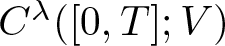 $C^\lambda([0,T];V)$. As in the above estimate, we obtain
 \begin{align*}
& \|\psi_{m_1+1}-\psi_{m_2+1}\|_{C_T^{0,\lambda} V}\\
& \le CT^{\gamma-\lambda} \|Y\|_{C_T^\gamma (\mathcal{L}_n(V))}
(\|\psi_0\|_V+\|\psi_{m_1}\|_{C_T^\lambda V}
+\|\psi_{m_2}\|_{C_T^\lambda V})^{n-1}
\|\psi_{m_1}-\psi_{m_2}\|_{C_T^{0,\lambda} V}
\end{align*}
for  $m_1,m_2\in{\mathbb{N}}$ and
 $0 \lt T \lt 1$. By choosing T > 0 sufficiently small, the claim follows. Moreover, there exists
 $\psi\in C^\lambda([0,T];V)$ such that
 $\|\psi_m-\psi\|_{C_T^{0,\lambda} V}\to 0$ as
 $m\to{\infty}$. Since
 $Y\in C^\gamma([0,T];\mathcal{L}_n(V))$, we see from the above estimate that
 \begin{align*}
\bigg\|\int_0^t Y_{d\tau}(\psi_m(\tau))
-\int_0^t Y_{d\tau}(\psi(\tau))\bigg\|_{C_T^{0,\gamma}V}
\to 0
\end{align*}
as  $m\to{\infty}$, which implies that ψ satisfies (2.1) for
 $0\le t\le T$. Notice that the solution is unique in
 $C^\lambda([0,T];V)$. Finally, following the above argument with a slight modification, we can obtain the continuous dependence. This completes the proof.
Remark 2.1.
In theorem 2.2, notice that  $\lambda \lt \gamma$ and
 $\gamma+\lambda \gt 1$ imply
 $\gamma \gt \frac12$. This corresponds to [Reference Chouk and Gubinelli7, theorem 2.4].
3. Multilinear estimates
In this section, we show the multilinear estimate which assures that our map X (defined in (1.6)) satisfies the assumption of theorem 2.2. We need to have an estimate of the following type:
Proposition 3.1.
Let  $d,k\in{\mathbb{N}}$ with
 $(d,k)\neq(1,1)$ and let
 $0 \lt \rho\le 1$. Let
 $s \gt s(\rho)=\frac d2-\frac{\rho}{k}$ and
 $-s\le s'\le s$. Then, for any
 $1\le q\le 2k+1$
 \begin{align}
\bigg\|\sum\limits_{\substack{n_1,\dots,n_{2k+1}\in{\mathbb{Z}}^d\\n_0-n_1+\dots-n_{2k+1}=0}}
\frac{1 }{{\langle {\Omega} \rangle }^\rho }
\prod\limits_{j=1}^{2k+1}\psi_j(n_j)\bigg\|_{\ell_{s'}^2({\mathbb{Z}}_{n_0}^d)}
\lesssim \|\psi_q\|_{\ell_{s'}^2}
\prod\limits_{\substack{j=1\\j\neq q}}^{2k+1}\|\psi_j\|_{\ell_s^2},
\end{align}
where  $\Omega=|n_0|^2-|n_1|^2+\cdots-|n_{2k+1}|^2$.
The following estimate corresponds to the case ρ = 0 in (3.1).
Lemma 3.2.
Let  $d,k\in{\mathbb{N}}$. Let
 $s\ge \frac d2$. Then, we have
 \begin{align}
\sum\limits_{\substack{n_0,n_1,\dots,n_{2k+1}\in{\mathbb{Z}}^d \\ n_0-n_1+\cdots-n_{2k+1}=0}}
\prod\limits_{j=0}^{2k+1}\psi_j(n_j)
\lesssim N_{\mathrm{max}}^{-2s}\prod\limits_{j=0}^{2k+1}N_j^s \|\psi_j\|_{\ell^2({\mathbb{Z}}^d)}
\end{align}
for any non-negative functions  $\{\psi_j\}_{j=0}^{2k+1}\subset\ell^2({\mathbb{Z}}^d)$ satisfying
 $\text{supp} \psi_j\subset\{n\in{\mathbb{Z}}^d:N_j\le {\langle {n} \rangle } \lt 2N_l\}$, where
 $N_{\mathrm{max}}:=\max_{0\le j\le 2k+1}N_j$. Here, the implicit constant is uniform in
 $\{N_j\}$.
Proof. By the symmetry, we may assume that
 \begin{align*}
N_0\ge N_2\ge \cdots\ge N_{2k},
\quad
N_1\ge N_3\ge \cdots \ge N_{2k+1},
\quad N_0\ge N_1.
\end{align*}
Note that  $N_{\mathrm{max}}=N_0\sim \max\{N_1,N_2\}$. Without loss of generality, we may assume that
 $N_{\mathrm{second}}=N_1$, where
 $N_{\mathrm{second}}$ is the second largest among
 $N_0,\ldots,N_{2k+1}$. The case
 $N_{\mathrm{second}}=N_2$ follows similarly: we only have to switch roles of ψ 1 and ψ 2. The Cauchy–Schwarz inequality and the Bernstein inequality show that the left-hand side of (3.2) is bounded by
 \begin{align*}
&\sum\limits_{n_1,\dots,n_{2k+1}\in{\mathbb{Z}}^d}\psi_{0}(n_1-n_2+\cdots+n_{2k+1})
\prod\limits_{j=1}^{2k+1}\psi_j(n_j)\\
&\le \|\psi_0\|_{\ell^2}\|\psi_1\|_{\ell^2}
\sum\limits_{n_2,\dots,n_{2k+1}\in{\mathbb{Z}}^d}\prod\limits_{j=2}^{2k+1}
\psi_j (n_j)
\lesssim \|\psi_0\|_{\ell^2}\|\psi_1\|_{\ell^2}
\prod\limits_{j=2}^{2k+1} N_j^{\frac d2}\|\psi_j\|_{\ell^2},
\end{align*}
which shows (3.2).
The following estimate is due to Kishimoto [Reference Kishimoto18], which corresponds to ρ > 1 in (3.1). Thanks to this strong decay of  ${\langle {\mu} \rangle }^{-\rho}$, we can obtain a better estimate than (3.2) with respect to the regularity.
Lemma 3.3. ([Reference Kishimoto18], lemma 3.1)
Let  $d,k\in{\mathbb{N}}$ with
 $(d,k)\neq(1,1)$. Let
 $s \gt s(1)=\frac d2-\frac{1}{k}$. Then, we have
 \begin{align}
\sum\limits_{\substack{n_0,n_1,\dots,n_{2k+1}\in{\mathbb{Z}}^d \\ n_0-n_1+\cdots-n_{2k+1}=0 \\ |n_0|^2-|n_1|^2+\cdots-|n_{2k+1}|^2=\mu}}
\prod\limits_{j=0}^{2k+1}\psi_j(n_j)
\lesssim N_{\mathrm{max}}^{-2s}\prod\limits_{j=0}^{2k+1}N_j^s \|\psi_j\|_{\ell^2({\mathbb{Z}}^d)}
\end{align}
for any  $\mu\in{\mathbb{Z}}$,
 $\{N_j\}_{j=0}^{2k+1}\subset 2^{{\mathbb{N}}_0}$, and any non-negative functions
 $\{\psi_j\}_{j=0}^{2k+1}\subset\ell^2({\mathbb{Z}}^d)$ satisfying
 $\text{supp} \psi_j\subset\{n\in{\mathbb{Z}}^d:N_j\le {\langle {n} \rangle } \lt 2N_l\}$, where
 $N_{\mathrm{max}}:=\max_{0\le j\le 2k+1}N_j$. Here, the implicit constant is uniform in µ and
 $\{N_j\}$.
Now, we prove proposition 3.1 by interpolating (3.2) and (3.3).
Proof of proposition 3.1
We mainly follow the proof of corollary 3.2 in [Reference Kishimoto18]. We only consider the case q = 1. Other cases follow from the same argument. By duality, if suffices to show
 \begin{align*}
\bigg|\sum\limits_{\substack{n_0,n_1,\dots,n_{2k+1}\in {\mathbb{Z}}^d\\n_0-n_1+\cdots-n_{2k+1}=0}}
\frac{1}{{\langle {\Omega} \rangle }^\rho}\prod\limits_{j=0}^{2k+1}\psi_j(n_j)\bigg|
\le C\|\psi_0\|_{\ell_{-s'}^2}\|\psi_1\|_{\ell_{s'}^2}
\prod\limits_{j=2}^{2k+1}\|\psi_j\|_{\ell_{s}^2},
\end{align*}
where  $\Omega=|n_0|^2-|n_1|^2+\cdots-|n_{2k+1}|^2$. We choose sufficiently small ɛ > 0 so that
 $s \gt s(\rho)+2\varepsilon$ and
 $k\varepsilon \lt \rho$. For this ɛ > 0, we also put
 $\theta:=\rho-k\varepsilon\in(0,1)$. We write
 $P_N\psi(n):={\mathbf 1}_{\{N\le {\langle {n} \rangle } \lt 2N\}}\psi(n)$. By the Hölder inequality in µ, the left-hand side of the above estimate is bounded by
 \begin{align*}
\begin{array}{ll}
&\sum\limits_{N_0,\dots,N_{2k+1}\in 2^{{\mathbb{N}}_0}}\sum\limits_{\mu\in{\mathbb{Z}}}
\sum\limits_{n_0,\dots,n_{2k+1}\in{\mathbb{Z}}^d}
\frac{{\mathbf 1}_{A(\mu)}}{{\langle {\mu} \rangle }^\rho}\prod\limits_{j=0}^{2k+1}|P_{N_j}\psi_j(n_j)|\\
&= \sum\limits_{N_0,\dots,N_{2k+1}}
\bigg(\sum\limits_{\mu\in{\mathbb{Z}}}\frac{1}{{\langle {\mu} \rangle }^{\rho}}
\bigg(\sum\limits_{n_0,\dots,n_{2k+1}\in{\mathbb{Z}}^d}{\mathbf 1}_{A(\mu)}\prod\limits_{j=0}^{2k+1}|P_{N_j}\psi_j(n_j)|\bigg)^{\theta}\\
&\quad\quad\quad\times
\bigg(\sum\limits_{n_0,\dots,n_{2k+1}\in{\mathbb{Z}}^d}{\mathbf 1}_{A(\mu)}\prod\limits_{j=0}^{2k+1}|P_{N_j}\psi_j(n_j)|\bigg)^{1-\theta}\bigg)\\
&\le \sum\limits_{N_0,\dots,N_{2k+1}}
\bigg(\sum\limits_{\mu\in{\mathbb{Z}}}\frac{1}{{\langle {\mu} \rangle }^{1+}}\sum\limits_{n_0,\dots,n_{2k+1}\in{\mathbb{Z}}^d}{\mathbf 1}_{A(\mu)}\prod\limits_{j=0}^{2k+1}|P_{N_j}\psi_j(n_j)|\bigg)^{\theta}\\
&\quad\quad\quad \times
\bigg(\sum\limits_{\mu\in{\mathbb{Z}}}\sum\limits_{n_0,\dots,n_{2k+1}\in{\mathbb{Z}}^d}{\mathbf 1}_{A(\mu)}\prod\limits_{j=0}^{2k+1}|P_{N_j}\psi_j(n_j)|\bigg)^{1-\theta}.
\end{array}
\end{align*}
Here,  $A(\mu)$ is defined by
 $A(\mu):=\{(n_0,n_1,\dots,n_{2k+1})\in({\mathbb{Z}}^d)^{2k+2}:(*)_\mu\}$, where ‘
 $(*)_\mu$’ denotes the condition
 \begin{align*}
n_0-n_1+\cdots-n_{2k+1}=0,\quad
\Omega=|n_0|^2-|n_1|^2+\cdots-|n_{2k+1}|^2=\mu.
\end{align*}
We also used  $\rho \gt \theta$. Note that
 $\theta (s(1)+\varepsilon)+\frac{(1-\theta) d}{2}=s(\theta)+\theta\varepsilon \lt s(\rho)+2\varepsilon$ since
 $\theta=\rho-k\varepsilon$. Notice that the value
 $\mu=|n_0|^2-|n_1|^2+\cdots-|n_{2k+1}|^2$ is determined once
 $n_0,\dots,n_{2k+1}$ are given. Thus, we have
 \begin{align*}
\sup_{n_0,\dots,n_{2k+1}\in{\mathbb{Z}}^d}\sum\limits_{\mu\in{\mathbb{Z}}}{\mathbf 1}_{A(\mu)}=1.
\end{align*}
Then, (3.2) with  $s=\frac d2$ and (3.3) with
 $s=s(1)+\varepsilon$ show that
 \begin{align*}
\begin{array}{ll}
&\lesssim \sum\limits_{N_0,\dots,N_{2k+1}}
\bigg(\frac{N_0N_1\cdots N_{2k+1}}{N_{\mathrm{max}}^2}\bigg)^{s(\theta)+\theta\varepsilon}\prod\limits_{j=0}^{2k+1}\|P_{N_j}\psi_j\|_{\ell^2}\\
&\lesssim \sum\limits_{N_0,\dots,N_{2k+1}} \bigg(\frac{N_0 N_1\cdots N_{2k+1}}{N_{\mathrm{max}}^2}\bigg)^{-\varepsilon'}
\|P_{N_0}\psi_0\|_{\ell_{-s'}^2}
\|P_{N_1}\psi_1\|_{\ell_{s'}^2}
\prod\limits_{j=2}^{2k+1}\|P_{N_j}\psi_j\|_{\ell_{s}^2},
\end{array}
\end{align*}
where  $\varepsilon'=s-s(\theta)-\theta\varepsilon \gt 0$. At the last inequality, we used
 $N_0^sN_1^s/N_{\mathrm{max}}^{2s}\le N_0^{-s'}N_1^{s'}$ for any
 $-s\le s'\le s$. For
 $N_{\mathrm{max}}$ and
 $N_{\mathrm{second}}\sim N_{\mathrm{max}}$, we can use the Cauchy–Schwarz inequality by orthogonality. Here,
 $N_{\mathrm{second}}$ is the second largest among
 $N_0,\ldots,N_{2k+1}$. On the other hand, summations over other Nj’s can be closed thanks to a negative power of Nj. This completes the proof.
4. Well-posedness
In this section, we prove our main result (theorem 1.2). For that purpose, we first investigate the property of our map X.
Proposition 4.1.
Let  $k,d\in {\mathbb{N}}$ with
 $(k,d)\neq (1,1)$ and
 $T,\rho,\gamma \gt 0$. Let
 $s \gt \frac d2-\frac{\rho}{k}$. Assume that a function
 $w\in C([0,T];{\mathbb{R}})$ is
 $(\rho,\gamma)$-irregular. Let X be defined in (1.6). Then, it holds that
 $X\in C^\gamma([0,T];\mathcal{L}_{2k+1}(H^s({\mathbb{T}}^d)))$.
Proof. Let  $\{\psi_j\}_{j=1}^{2k+1}\subset H^s({\mathbb{T}}^d)$. We see from proposition 3.1 that
 \begin{align*}
&\|X_{t_1;t_2}(\psi_1,\ldots,\psi_{2k+1})\|_{H^s}\\
&=\bigg\|\int_{t_1}^{t_2}\sum\limits_{n_1,\dots,n_{2k+1}\in{\mathbb{Z}}^d}
{\langle {n} \rangle }^{s}e^{-iw(\tau)\Omega}
{\mathbf 1}_{\{n=\sum\limits_{j=1}^{2k+1}\zeta_j n_j\}}
\prod\limits_{j=1}^{2k+1}J_j\hat{\psi}_{j}(n_{j})
d\tau\bigg\|_{\ell^2({\mathbb{Z}}_n^d)}\\
&\lesssim \|\Phi^w\|_{\mathcal{W}_T^{\rho,\gamma}}|t_2-t_1|^\gamma
\bigg\|\sum\limits_{n_1,\dots,n_{2k+1}\in{\mathbb{Z}}^d}
\frac{{\langle {n} \rangle }^{s}{\mathbf 1}_{\{n=\sum\limits_{j=1}^{2k+1}\zeta_j n_j\}}}{{\langle {\Omega} \rangle }^\rho}
\prod\limits_{j=1}^{2k+1}|\hat{\psi}_j(n_{j})|\bigg\|_{\ell^2({\mathbb{Z}}_n^d)}\\
&\lesssim \|\Phi^w\|_{\mathcal{W}_T^{\rho,\gamma}}|t_2-t_1|^\gamma
\prod\limits_{j=1}^{2k+1}\|\psi_j\|_{H^s},
\end{align*}
where  $\Omega=|n|^2-\sum\limits_{j=1}^{2k+1}\zeta_j|n_j|^2$,
 $\zeta_{2j-1}=+$,
 $\zeta_{2j}=-$,
 $J_{2j-1}\psi=\psi$ and
 $J_{2j}\psi=\bar{\psi}$ for a function ψ. Then, we have
 \begin{align*}
\|X\|_{C^\gamma ([0,T];\mathcal{L}_{2k+1}(H^s))}
=\sup_{0\le s \lt t\le T}\sup_{\psi_j\in H^s}
\frac{\|X_{s;t}(\psi_1,\ldots,\psi_{2k+1})\|_{H^s}}{|t-s|^\gamma \prod_{j=1}^{2k+1}\|\psi_j\|_{H^s}}
\lesssim \|\Phi^w\|_{\mathcal{W}_T^{\rho,\gamma}} \lt \infty
\end{align*}
as desired. This completes the proof.
Now, we are ready to prove our main result (theorem 1.2).
Proof of theorem 1.2
Let X be defined in (1.6). Proposition 4.1 implies that  $X\in C^\gamma([0,T_0]; \mathcal{L}_{2k+1}(H^s({\mathbb{T}}^d)))$ for any
 $T_0 \gt 0$. From the definition of X, it is clear that
 $X_0(\psi)=0$ for any
 $\psi\in H^s({\mathbb{T}}^d)$. Then, theorem 2.2 shows that there exists
 $T\in(0,T_0)$ depending only on
 $\|X\|_{C^\gamma([0,T_0];\mathcal{L}_{2k+1}(H^s({\mathbb{T}}^d)))}$ and
 $\|\varphi_0\|_{H^s}$ such that there exists a unique solution
 $\varphi\in C^\lambda([0,T];H^s({\mathbb{T}}^d))$ to (1.7), which completes the proof.
Acknowledgements
The author appreciates the valuable comments provided by the anonymous referee. The author is grateful to Professor Yuzhao Wang for suggesting this problem and fruitful discussion. He also thanks Professor Tristan Robert for letting the author know the paper [Reference Kishimoto17]. The author was supported by the EPSRC New Investigator Award (grant no. EP/V003178/1), Iizuka Takeshi Scholarship Foundation, JSPS KAKENHI Grant Number 23K19019, and a grant from the Harris Science Research Institute of Doshisha University.



