2. Formulation

Consider a gaseous reactant–oxidiser mixture at rest with given density $\rho _0$ , temperature $T_0$ and mass fractions of fuel and oxidiser, $Y_{F0}$ and $Y_{O0}$ , respectively, which is bounded by a wall in a half-space. We consider a planar configuration in which all variables depend only on one spatial coordinate, $x^\prime$ , and time, $t^\prime$ . Here and below, the prime symbols denote dimensional quantities if the same letters are used for dimensional and dimensionless quantities. The low Mach number approximation is adopted in the present study. For simplicity, changes in the thermal conductivity, $\lambda$ , the fuel diffusion, $\mathcal D$ , and the specific heat (at constant pressure), $c_{\!p}$ , of the mixture are neglected. In the following, the thermal diffusion coefficient is based on the initial density of the mixture, ${\mathcal D}_T=\lambda /\rho _0 c_{\!p}$ .

The ignition process is initiated by a change in the wall temperature condition. We consider two cases. In the first case, the ignition process is initiated by heat release from the wall for a finite time $t^\prime _*$ , with intensity $H_w$ . After this time the wall becomes adiabatic. In the second case the ignition process is produced by a change in the wall temperature, $T|_{x=0}=T_w(t^\prime )$ .

In the present study, the lean flammability limit is defined as the limit of fuel concentration and temperature below which a solution in the form of a planar combustion wave does not exist. This can be achieved by setting a critical cutoff temperature, $T_c$ , below which the rate of fuel conversion into products vanishes. This effect is present, for instance, in the two-step chain-branching model proposed in Dold et al. (Reference Dold, Thatcher, Omon-Arancibia and Redman2002) and Dold (Reference Dold2007). Within this model, there is a cross-over temperature below which the rate of radical removal by diffusion exceeds the rate of chain branching. In the present study, however, we use a simpler global irreversible one step reaction of the form

(2.1) \begin{align} \text{Fuel} + \text{Oxidizer} \to \text{Products} + \text{Heat} \end{align}

that proceeds at a rate $\omega ^\prime \sim {\mathcal B}(\rho ^\prime Y_{\!F}/W_{\!F})\boldsymbol{\cdot }(\rho ^\prime Y_O/W_O)$ . In the model used in this study, the rate of the fuel-to-products transformation becomes zero below a certain temperature, i.e. when $T\lt T_c$ , as specified below. Here, ${\mathcal B}$ is the pre-exponential factor, $\rho ^\prime$ is the mixture density, while $Y_{\!F}$ , $Y_O$ , $W_{\!F}$ , $W_O$ denote the mass fractions and molecular weights of the fuel and oxidiser.

For simplicity, we assume that the mixture is lean in fuel and denote its mass fraction by $Y$ , treating the oxidiser mass fraction as a constant absorbed in $\mathcal B$ together with the fuel and oxidiser molecular weights. We want to formulate a reaction rate model for which, if the adiabatic (maximum) temperature achieved in a hypothetical planar combustion wave propagating at a constant velocity with respect to the unburned gas, $T_a=T_0+Q Y_0/c_{\!p}$ , where $Q$ is the heat release per unit fuel mass, is lower than the cutoff temperature, $T_a\lt T_c$ , then a standard planar wave solution does not exist.

Two different models are proposed here to describe this dependence of the fuel consumption rate on temperature. In the first case, we use a stepwise (Heaviside) dependence, $\omega ^\prime ={\rho ^\prime }^2{\mathcal B}Y \textrm {Hev} (T-T_c)$ . In the second model, the standard Arrhenius kinetics $\omega ^\prime ={\rho ^\prime }^2{\mathcal B}Y\exp \{{\mathcal E}/{\mathcal R}T_c-{\mathcal E}/{\mathcal R}T\}$ for $T\gt T_c$ is used. Here, $\mathcal E$ is the overall activation energy and $\mathcal R$ is the universal gas constant. As will be seen below, the specific dependence of the reaction rate on temperature at $T\gt T_c$ turns out to be irrelevant for the new mode of combustion wave propagation described in the present work.

Dimensionless variables are introduced as follows:

(2.2) \begin{equation} \begin{array}{c} \theta =(T-T_0)/(T_c-T_0),\quad Y=Y^\prime /Y_0, \quad \rho =\rho ^\prime /\rho _0,\\[9pt] t=t^\prime /t_c,\quad x=x^\prime /\ell _c,\quad u=u^\prime /u_c,\\ \end{array} \end{equation}

where the scales for time $t_c$ , distance $\ell_c$ , and speed $u_c$ , are determined from the relationships

(2.3) \begin{equation} t_c=\ell _c^2/{\mathcal D}_T,\quad t_c\rho _0{\mathcal B}=k_0,\quad u_c=\ell _c/t_c. \end{equation}

The dimensionless governing equations take the form

(2.4) \begin{equation} {\partial \rho \over \partial t}+{\partial (\rho u)\over \partial x}=0, \end{equation}

(2.5) \begin{equation} \rho {\partial \theta \over \partial t}+\rho u {\partial \theta \over \partial x}={\partial ^2\theta \over \partial x^2}+q\omega , \end{equation}

(2.6) \begin{equation} \rho {\partial Y\over \partial t}+\rho u {\partial Y\over \partial x}={1\over \textit{Le}}{\partial ^2 Y\over \partial x^2}-\omega , \end{equation}

(2.7) \begin{equation} \rho (1+\alpha \theta )=1, \end{equation}

where the last equation represents the equation of state of an ideal gas. As is usual within the zero Mach approximation applied to the one-dimensional dynamics, the equation for conservation of momentum is not required. Given the distributions of the variables, the equation determining the velocity field can be written as follows:

(2.8) \begin{equation} {\partial u\over \partial x}=\alpha \left({\partial ^2 \theta \over \partial x^2}+q\omega \right)\!. \end{equation}

This equation, obtained by manipulating (2.4)–(2.5) and (2.7), is used instead of (2.4) in what follows.

The dimensionless reaction rate takes the form $\omega =\rho ^2\,K(\theta )Y$ , where

(2.9) \begin{equation} K(\theta )=\left \{ \begin{array}{ll} k(\theta ),\quad &\theta \geqslant 1,\\[5pt] 0,\quad &\theta \lt 1,\\ \end{array}\right . \end{equation}

with $k(\theta )=k_0$ or $k(\theta )=k_0\exp \{\beta (\theta -1)/[1+\gamma (\theta -1)]\}$ for the stepwise and the Arrhenius kinetics, respectively. Note that the dimensionless cutoff temperature is defined as $\theta _c=1$ in this notation and as such appears in the expressions of the dimensionless reaction rates.

The following initial and boundary conditions are imposed. In the case of an imposed heat flux from the wall, we have

(2.10) \begin{equation} x=0:\, {\partial \theta /\partial x}=\left \{ \begin{array}{ll} -h_w,\, &t\lt t_*,\\[5pt] 0,\, &t\geqslant t_*,\\ \end{array}\right . \, {\partial Y/\partial x}=0,\quad u=0. \end{equation}

Obviously, to achieve ignition below flammability using a prescribed wall temperature, this value must exceed the cutoff temperature at least at some initial time. For this reason, the following boundary conditions were used in the case of imposed wall temperature:

(2.11) \begin{equation} x=0:\,\theta =\left \{ \begin{array}{ll} \theta _{*},\quad &t\lt t_*,\\[5pt] \theta _{w},\quad &t\geqslant t_*,\\ \end{array}\right . \quad {\partial Y/\partial x}=0,\,\quad u=0, \end{equation}

where $\theta _{*}\gt 1$ was applied. This dependence ensures ignition of the mixture at the beginning of the combustion process.

For the initial conditions and conditions far from the wall, we use

(2.12) \begin{equation} t=0:\quad \theta =0,\quad Y=1, \end{equation}

(2.13) \begin{equation} x\to \infty :\quad {\partial \theta /\partial x}={\partial Y/\partial x}=0. \end{equation}

The initial distribution for the velocity field, $u$ , is not required within the low Mach approximation, since the velocity at each moment of time is determined from (2.8). The boundary conditions at $x\to \infty$ , defined by (2.13), are imposed in a weak form. This choice does not affect the results presented below, since the initial distributions defined by (2.12) satisfy them.

The following non-dimensional parameters appear in the above formulation: the Zel’dovich number, $\beta ={\mathcal E}(T_c-T_0)/{\mathcal R}T_c^2$ , the fuel Lewis number, $\textit{Le}={\mathcal D}_T/{\mathcal D}$ , the heat expansion parameter, $\alpha =(T_c-T_0)/T_0$ , the dimensionless heat of reaction, $q=QY_0/[c_{\!p}(T_c-T_0)]$ , the dimensionless heat flux emitted by the wall, $h_w=\ell _c H_w/\lambda (T_c-T_0)$ , the dimensionless time of wall heating action, $t_*=t^\prime _*/t_c$ , appearing in (2.10), and the dimensionless pre-exponential factor, $k_0$ , given by (2.3). Below, we use $k_0=\beta ^2$ in order to have a dimensionless velocity of the planar front (when it exists) of the order of unity as $\beta \to \infty$ in the case of the Arrhenius kinetics. Anticipating the results of the asymptotic analysis presented in § 5, the choice of $k_0$ is irrelevant for the $t\gg 1$ dynamics below the flammability limit.

It should be noted that, strictly speaking, the heat-release parameter $\gamma$ appearing in (2.9) for the Arrhenius kinetics and the $\alpha$ parameter in (2.7) are related by the equation $\gamma = \alpha / (\alpha + 1)$ . However, in the limit of the constant-density approximation (the diffusion–thermal approximation), when $\alpha \to 0$ , the temperature dependence of the reaction rate in the case of Arrhenius kinetics is still written as $k(\theta )=k_0\exp \{\beta (\theta -1)/ [1+\gamma (\theta -1)]\}$ in many studies. In this sense, $\gamma$ plays the role of an independent parameter characterising the kinetics. For this reason, to ensure the generality of the results, we also consider $\alpha$ and $\gamma$ as two independent parameters.

To characterise the combustion dynamics, we track the flame position, $x_{\!f}$ , defined as the point where the temperature is equal to unity, $\theta |_{x=x_{\!f}}=1$ . In cases where there are two such points, the one located closer to the fresh mixture is selected. Looking ahead, these cases are observed in calculations with a fixed wall temperature smaller than one. Numerical calculations show that at this point the reaction rate reaches its maximum value.

Note that, with the chosen dimensionless variables, the flame adiabatic temperature is equal to $q$ . This value is achieved in a planar combustion front with complete fuel consumption propagating at a constant velocity relative to the fresh mixture (when it exists). The values $\beta =10$ and $\gamma =0.7$ are chosen as representative values, while $\textit{Le}$ , $q$ and $\alpha$ are varied.

3. Numerical treatment

For a given heat flux at the wall (i.e. the boundary conditions given by (2.10)) and for the case in which chemical reactions are neglected (i.e. $\omega \equiv 0$ ), the temperature field at $t\ll 1$ is described by the well-known analytical solution

(3.1) \begin{equation} \theta =h_w t^{1/2}\{2e^{-\eta ^2/4}/\sqrt {\pi }-\eta [1-\textrm {erf}(\eta /2)]\}, \end{equation}

where $\eta =x/t^{1/2}$ , and $\textrm {erf}(\boldsymbol{\cdot })$ is the error function. When the wall temperature increases sharply from $0$ to $\theta _*$ , the temperature distribution can be written for $\alpha =0$ in analytical form as

(3.2) \begin{equation} \theta =\theta _*[1-\textrm {erf}(\eta /2)]. \end{equation}

Thus, immediately after wall heating, at $t\ll 1$ , the heated region is small, of order $O(t^{1/2})$ . In order to take this into account, the transformation $x=\eta e^{\tau /2}$ , $t=e^{\tau }$ is applied. Using these new variables, (2.5)–(2.6) and (2.7) become

(3.3) \begin{equation} \rho \left[{\partial \theta \over \partial \tau }+ \left(V-{\eta \over 2} \right){\partial \theta \over \partial \eta } \right]={\partial ^2 \theta \over \partial \eta ^2}+q \omega e^{\tau }, \end{equation}

(3.4) \begin{equation} \rho \left[{\partial Y\over \partial \tau }+ \left(V-{\eta \over 2}\right){\partial Y\over \partial \eta } \right]={1\over \textit{Le}}{\partial ^2 Y\over \partial \eta ^2}-\omega e^{\tau }, \end{equation}

(3.5) \begin{equation} {\partial V\over \partial \eta }=\alpha \left[{\partial ^2\theta \over \partial \eta ^2} +q\omega e^\tau \right]\!, \end{equation}

where $V=t^{1/2}u$ is introduced for the velocity variable. Equations (3.3)–(3.5) also indicate that at $t\ll 1$ , or at $\tau \to -\infty$ , the contribution of the combustion reaction is small, since the reaction rate $\omega$ remains finite.

The computations were carried out in a finite domain of $0\le \eta \le \eta _{\textit{max}}$ and the initial condition given by (2.12) was imposed at $\tau =\tau _{\textit{min}}$ . Typical values of $\eta _{\textit{max}}=15\div 20$ and $\tau _{\textit{min}}=-(10\div 15)$ were used. All the numerical results reported below were obtained using second-order, three-point central differences for spatial derivatives on a rectangular uniform grid with a typical resolution of $\delta \eta =\eta _{\textit{max}}/4000$ . The presence of the highly nonlinear reaction rate terms required us to choose a sufficiently small time step, $\delta \tau =10^{-6}$ . The independence of the results on $\delta \eta$ and $\delta \tau$ was verified specifically.

4. Numerical results

In cases where the combustion front formed after successful ignition propagates at a constant velocity $u_{\!p}$ , a reference frame associated with the front is typically used, namely, the $x^\prime \to x-u_{\!p}t$ transformation. Omitting the primes, (2.5)–(2.6) are written as

(4.1) \begin{equation} m{\text{d}\theta \over \text{d}x}={\text{d}^2\theta \over \text{d}x^2}+q\omega , \end{equation}

(4.2) \begin{equation} m{\text{d} Y\over \text{d}x}={1\over \textit{Le}}{\text{d}^2 Y\over \text{d}x^2}-\omega , \end{equation}

were $m=\rho (u-u_{\!p})$ is a constant. This value determines the flame velocity with respect to the unburned gas. The (negative) value of $m$ represents the eigenvalue of the problem, to be determined from (4.1)–(4.2) subject to the boundary conditions

(4.3) \begin{equation} x\to \infty :\quad \theta =Y-1=0;\quad x\to -\infty :\quad \text{d}\theta /\text{d}x=\text{d}Y/\text{d}x=0, \end{equation}

if the flame propagates from left to right.

The well-known first integral of this problem

(4.4) \begin{equation} m(\theta +qY)={\text{d}\theta \over \text{d}x}+{q\over \textit{Le}}{\text{d}Y\over \text{d}x}+mq, \end{equation}

allows us to get the temperature behind the flame, $\theta _{x\to -\infty }=q(1-Y_{x\to -\infty })$ , where $Y_{x\to -\infty }\geqslant 0$ is the value of possible fuel leakage. From (4.1) it can be obtained that

(4.5) \begin{align} {\text{d}\theta \over \text{d}x}=-q\int \limits _{-\infty }^x \omega e^{-m(\xi -x)}\text{d}\xi \lt 0 \end{align}

and the temperature decreases monotonically with $x$ . Thus, the value of $\theta _{x\to -\infty }$ corresponds to the maximum temperature for the combustion front propagating with a constant velocity. Therefore, if $q\lt 1$ , the maximum temperature of the hypothetical flame becomes less than the cutoff temperature, which is equal to unity. It means that for $q\lt 1$ the solution of (2.5)–(2.6) in the form of a planar combustion front propagating at a constant velocity does not exist.

4.1. Imposed heat flux from the wall

Numerical calculations based on (3.3)–(3.5) subject to the boundary conditions specified by (2.10) were carried out for $q\lt 1$ . For all the cases described below, when specifying the wall heat flux determined by (2.10), the values $h_w=1.2$ and $t_*=1$ were used. Remember that the boundary conditions at the wall become adiabatic as $t\gt t_*$ . Figure 1 shows the flame position versus time obtained using the stepwise reaction model. In the left plot, the solid curves correspond to $q=0.7$ and various $\alpha$ values. In the right plot, the value of $q$ is varied, while $\alpha =5$ is maintained for all curves. The vertical dotted-dashed line indicates the time of wall heating, $t_*$ , after which the wall becomes adiabatic. Anticipating the asymptotic results presented in § 5, the dashed lines show the asymptotic dependencies of the flame position on time at $t\gg 1$ .

Figure 1.

Flame position versus time calculated for the stepwise kinetics and various parameter values with the boundary given by (2.10). (a) The plot shows curves calculated for $q = 0.7$ and various $\alpha$ ; (b) curves for $\alpha = 5$ and various $q$ . The vertical dashed–dotted line indicates the value of $t_*$ . The dashed lines show the asymptotic dependencies $x_{\!f}=At^{1/2}$ described in § 5 for $t\gg 1$ .

Figure 1. Long description

Two line graphs depict the flame position over time for different parameter values. Panel A: The left graph shows curves calculated for Le equal to 0.3 and q equal to 0.7 with varying alpha values of 0, 3, and 5. The x-axis represents time (t) in logarithmic scale ranging from 10^−2 to 10^6, and the y-axis represents the flame position (x_f) in logarithmic scale ranging from 10^−1 to 10^4. The vertical dashed-dotted line indicates the value of t equal to 1. The dashed lines show the asymptotic dependencies described in the reference for alpha equal to 0. Panel B: The right graph shows curves for Le equal to 0.3 and alpha equal to 5 with varying q values of 0.5, 0.6, and 0.7. The x-axis represents time (t) in logarithmic scale ranging from 10^−2 to 10^6, and the y-axis represents the flame position (x_f) in logarithmic scale ranging from 10^−1 to 10^4. The vertical dashed-dotted line indicates the value of t equal to 1. The dashed lines show the asymptotic dependencies described in the reference for q equal to 0.5.

Figure 2 illustrates the distributions of temperature, mass fraction of fuel, reaction rate and gas velocity obtained for $q=0.7$ , $\alpha =2$ and $\textit{Le}=0.3$ presented for different times during flame propagation. It can be seen that the reaction rate distributions become narrower and narrower at long times when compared with the characteristic lengths of temperature or mass fraction changes. Another important observation is that at $t\gg 1$ , in the region between the wall and the flame, $0\lt x\lt x_{\!f}$ , the temperature, mass fraction and velocity fields are practically uniform, namely $\theta \approx 1$ , $Y\approx 0$ and $V\approx 0$ .

Figure 2.

Distributions of temperature, fuel mass fraction and reaction rate plotted for different moments of time, for $\alpha =2$ , $q=0.7$ and $\textit{Le}=0.3$ , calculated with the boundary conditions given by (2.10).

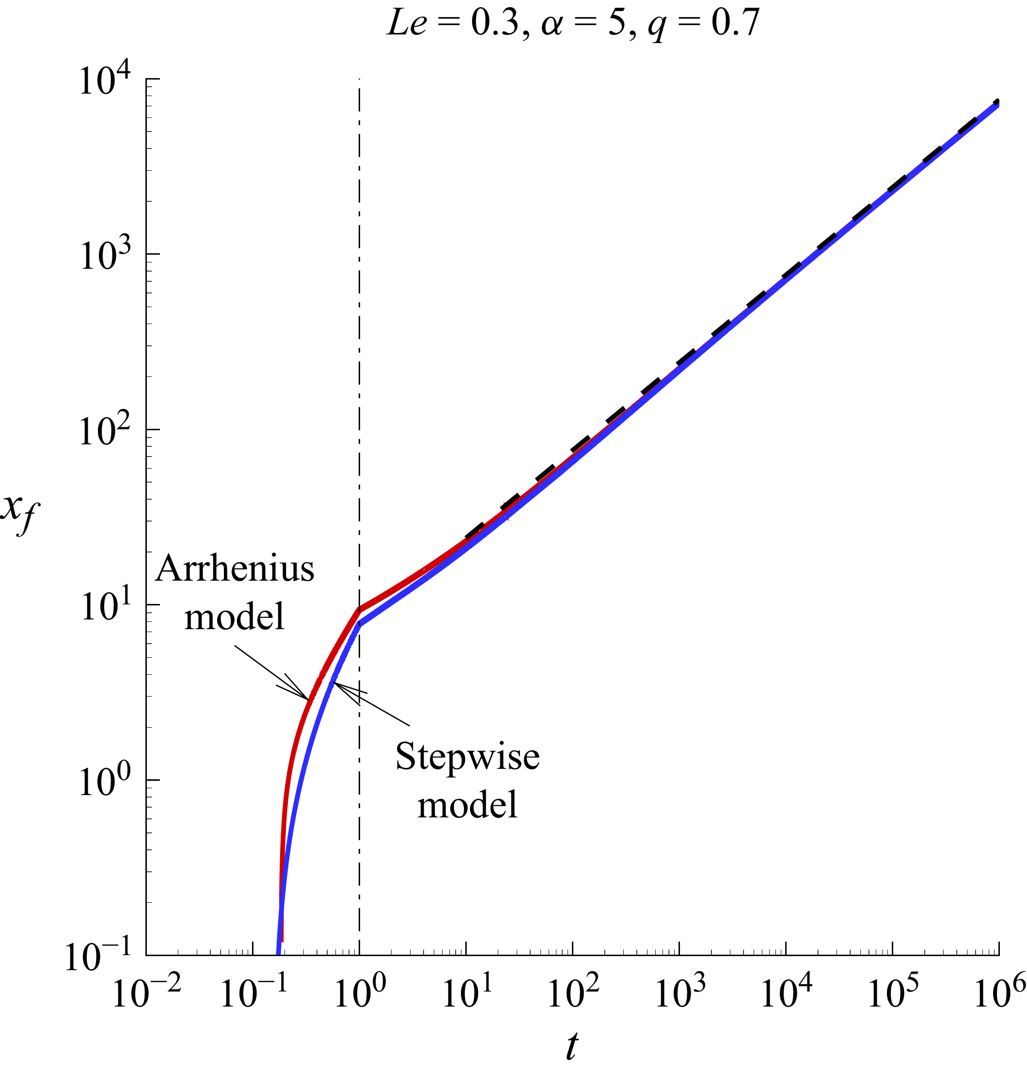
All the results presented in figures 1 and 2 were obtained for the stepwise reaction rate model, namely when $K(\theta ) = k_0$ for $\theta \gt 1$ was used in (2.9). Figure 3 compares the flame position dependencies on time obtained for the stepwise and Arrhenius models. It can be seen that, although the flame positions $x_{\!f}$ calculated within these two models differ slightly after the heating action ceases, at sufficiently long times the curves overlap. This means that the specific dependence of $K(\theta )$ for $\theta \gt 1$ is not relevant when $t\gg 1$ .

Figure 3.

Comparison of flame position versus time obtained for the stepwise and Arrhenius dependencies, calculated with the wall boundary conditions in (2.10). The vertical dashed–dotted line indicates the value of $t_*=1$ . The dashed lines show the asymptotic dependencies $x_{\!f}=At^{1/2}$ obtained for $t\gg 1$ in § 5.

4.2. Imposed wall temperature dependence

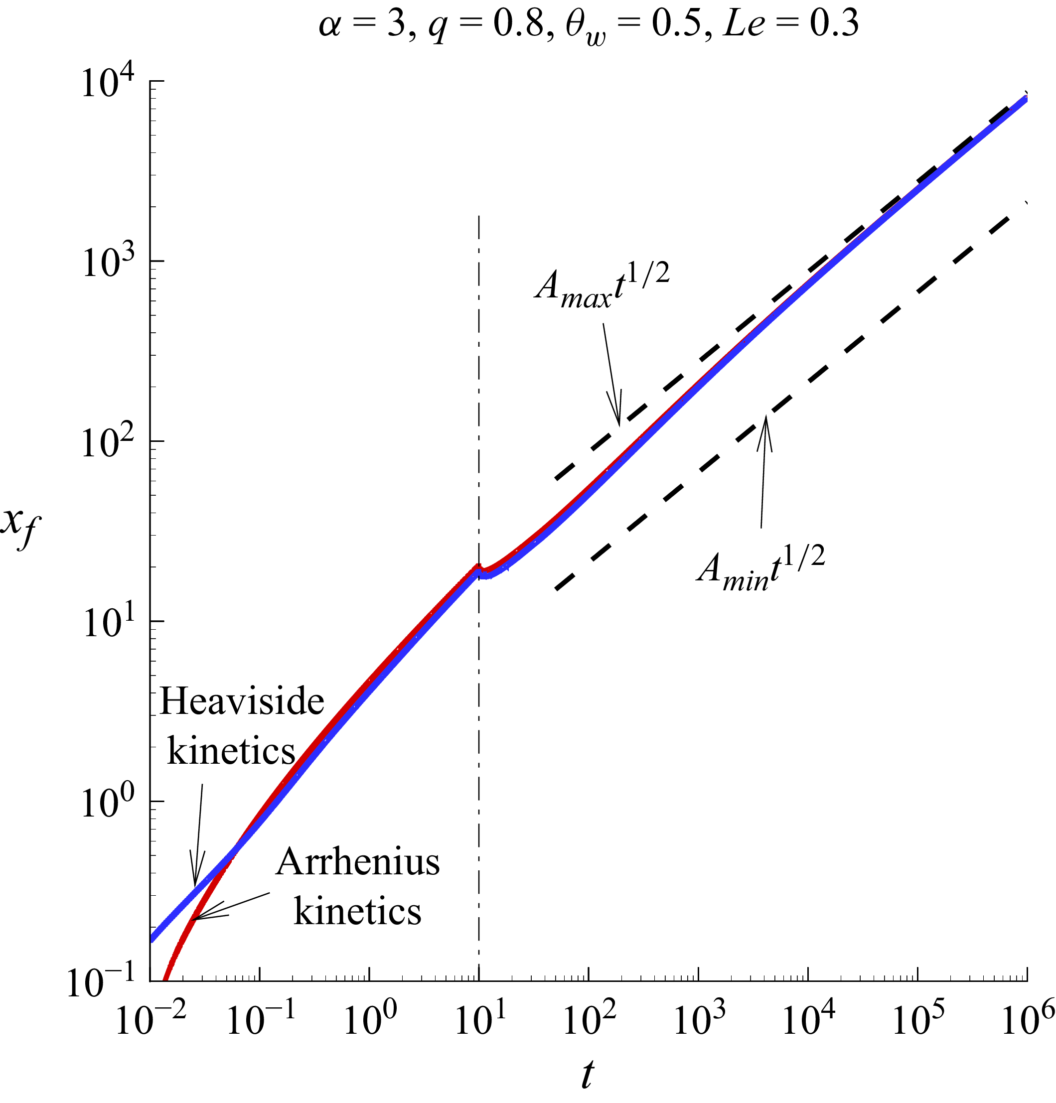
For calculations with the law for wall temperature given by (2.11), the values $t_*=10$ and $\theta _{*}=2$ were used in the numerical calculations reported here. Figure 4 shows the evolution of the flame positions relative to the wall obtained for the stepwise and Arrhenius reaction rate models. It can be seen that, as in the case of a given heat flux, the curves overlap at $t\gg 1$ . The temperature, fuel mass fraction, reaction rate and gas velocity profiles are shown in figure 5, calculated for some time instants in the case of the Arrhenius model for $K(\theta )$ . It can be noted that in this case the gas velocity distribution does not become close to zero, instead, it is negative between the flame front and the wall.

Figure 4.

Flame position versus time obtained for the stepwise and Arrhenius dependencies for $K(\theta )$ for $\alpha =3$ and $\theta _w=0.5$ calculated with the boundary conditions in (2.11). The vertical dashed–dotted line indicates the value of $t_*=10$ . The dashed lines show the asymptotic dependencies $x_{\!f}=A_{\textit{min}}t^{1/2}$ and $x_{\!f}=A_{\textit{max}}t^{1/2}$ obtained for $t\gg 1$ in § 5.

Figure 5.

Distributions of temperature, fuel mass fraction and reaction rate plotted for different moments of time, for $\alpha =3$ , $\theta _w=0.5$ , $q=0.8$ and $\textit{Le}=0.3$ , calculated with the boundary conditions given by (2.11).

Figure 5. Long description

Three line graphs depict the distributions of temperature, fuel mass fraction, and reaction rate over time. Panel A: The line graph shows the distributions at t = 10^2. The x-axis represents the spatial coordinate ranging from 0 to 150, and the y-axis on the left represents the normalized temperature (θ), fuel mass fraction (Y), and reaction rate (ω), while the y-axis on the right represents the velocity (V). The red line indicates the temperature distribution, the blue line indicates the fuel mass fraction, the green line indicates the velocity, and the black line indicates the reaction rate. Panel B: The line graph shows the distributions at t = 10^4. The x-axis represents the spatial coordinate ranging from 0 to 2000, and the y-axes are the same as in Panel A. The red line indicates the temperature distribution, the blue line indicates the fuel mass fraction, the green line indicates the velocity, and the black line indicates the reaction rate. Panel C: The line graph shows the distributions at t = 10^6. The x-axis represents the spatial coordinate ranging from 0 to 20000, and the y-axes are the same as in Panel A. The red line indicates the temperature distribution, the blue line indicates the fuel mass fraction, the green line indicates the velocity, and the black line indicates the reaction rate.

5. Asymptotic description for $\boldsymbol{t\gg 1}$

Figures 3 and 4 demonstrate that as $t\gg 1$ , the flame position versus time becomes independent of the specific type of kinetics appearing in (2.9), namely the dependence of $K(\theta )$ for $\theta \gt 1$ . In turn, the profiles of the variables at long times, shown in figures 2 and 5, indicate that the reaction rate, $\omega$ , acts as a Dirac delta function in the combustion zone occurring at $\theta \approx \theta _c$ (equal to unity). Thus, we can write

(5.1) \begin{equation} \omega =B\delta (x-x_{\!f}),\quad \textrm {where}\quad B={1\over \textit{Le}}{\partial Y\over \partial x}\bigg |_{x=x_{\!f}+0}. \end{equation}

To find the solution for $t\gg 1$ , it is convenient to transform the coordinates by introducing $\xi =(x-x_{\!f}(t))/\sqrt {t}$ in (2.5)–(2.6) and (2.8), where $x_{\!f}(t)$ is the flame position. Thus, the combustion front is fixed at $\xi =0$ . The resulting equations take the form

(5.2) \begin{equation} t\rho {\partial \theta \over \partial t}+\rho \bigg (V-{\text{d}x_{\!f}\over \text{d}t}\sqrt {t} -{\xi \over 2}\bigg ){\partial \theta \over \partial \xi } ={\partial ^2\theta \over \partial \xi ^2}+t q \omega, \end{equation}

(5.3) \begin{equation} t\rho {\partial Y\over \partial t}+\rho \bigg (V-{\text{d}x_{\!f}\over \text{d}t}\sqrt {t} -{\xi \over 2}\bigg ){\partial Y\over \partial \xi } ={1\over \textit{Le}}{\partial ^2 Y\over \partial \xi ^2}-t\omega , \end{equation}

(5.4) \begin{equation} {\partial V\over \partial \xi }=\alpha \bigg ({\partial ^2\theta \over \partial \xi ^2}+tq\omega \bigg ). \end{equation}

Finally, for the reaction rate multiplied by time, one can write that

(5.5) \begin{equation} t\,\omega =\tilde B\delta (\xi ),\quad \textrm {where}\quad \tilde B={1\over \textit{Le}}{\partial Y\over \partial \xi }\bigg |_{\xi =0+}, \end{equation}

where the property of the Dirac delta function, $\delta (az)=a^{-1}\delta (z)$ , was used.

The boundary conditions that need to be added to (5.2)–(5.4) are

(5.6) \begin{equation} \begin{array}{ll} \xi =-\xi _{\!f}:\quad & \left \{ \begin{array}{l} {\partial \theta /\partial x}=0,\\[5pt] \theta =\theta _w, \\[5pt] \end{array}\right . \quad {\partial Y/\partial \xi }=0,\quad V=0, \\[11pt] \xi \to \infty :\quad &\theta =0,\quad Y=1,\\ \end{array} \end{equation}

where $\xi _{\!f}=x_{\!f}/\sqrt {t}$ . The upper and lower conditions for the temperature field at $\xi =-\xi _{\!f}$ correspond to the case of the adiabatic wall and the case of the fixed wall temperature, respectively. The conditions for temperature and fuel mass fraction at the flame front are

(5.7) \begin{equation} \xi =0:\quad \theta =1,\quad Y=0. \end{equation}

The presence of the $\delta$ -function in (5.2)–(5.4) is equivalent to the following conditions:

(5.8) \begin{equation} \parallel {\partial \theta /\partial \xi }\parallel +q \parallel {\partial Y/\partial \xi }\parallel /\textit{Le}=0, \quad \parallel V \parallel =0, \end{equation}

where $\parallel f \parallel =f(0+)-f(0-)$ . These conditions are obtained by integrating of (5.2)–(5.4) around $\xi =0$ and eliminating $\tilde B$ .

Let’s assume that, in the first approximation,

(5.9) \begin{equation} x_{\!f}(t)=A t^{1/2},\quad \theta =\theta _0(\xi ),\quad Y=Y_0(\xi ),\quad V=V_0(\xi ), \end{equation}

where the value of $A$ is to be determined. Substituting these expressions into (5.2)–(5.4) we have the following equations:

(5.10) \begin{equation} \left \{ \begin{array}{l} \displaystyle \rho _0\bigg (V_0-{\xi +A\over 2}\bigg ){\text{d}\theta _0\over \text{d}\xi }={\text{d}^2\theta _0\over \text{d}\xi ^2},\\[12pt] \displaystyle \rho _0\bigg (V_0-{\xi +A\over 2}\bigg ){{\rm d} Y_0\over \text{d}\xi }={1\over \textit{Le}} {\text{d}^2 Y_0\over \text{d}\xi ^2},\\[12pt] \displaystyle {{\rm d} V_0\over \text{d}\xi }=\alpha {\text{d}^2\theta _0\over \text{d}\xi ^2},\\ \end{array}\right . \end{equation}

where $\rho _0=(1+\alpha \theta _0)^{-1}$ .

Equations (5.10) are to be solved subject to the boundary conditions

(5.11) \begin{equation} \begin{array}{lll} \displaystyle \xi =-A:\quad & \left \{\begin{array}{l} \text{d}\theta _0/\text{d}\xi =0,\\[7pt] \theta _0=\theta _w,\\ \end{array}\right . \quad &{\text{d} Y_0/\text{d}\xi }=0,\quad V_0=0,\\[12pt] \xi =0:\quad &\theta _0=1,\quad &Y_0=0,\\[12pt] \xi \to \infty :\quad &\theta _0=0,\quad &Y_0=1,\\ \end{array} \end{equation}

where again the upper and lower conditions for the temperature field at $\xi = -A$ correspond to the case of the adiabatic wall and the case of the fixed wall temperature. Additionally, the conditions in (5.8) should be fulfilled. The value $A$ represents the eigenvalue of the problem, similar to the value of the propagation speed of the combustion wave when it exists in the standard mode.

It can be immediately seen that $Y_0\equiv 0$ for $-A\lt \xi \lt 0$ . Indeed, if we formally write from (5.10) that

(5.12) \begin{align} {{\rm d} Y_0\over \text{d}\xi }=C\exp \bigg (\textit{Le} \int \limits _{-A}^\xi \rho _0 [V_0-(\tilde \xi +A)/2]\text{d}\tilde \xi \bigg )\quad \textrm {for}\quad -A\lt \xi \lt 0, \end{align}

then from the boundary condition it follows that $C\equiv 0$ .

In the general cases, for $\alpha \ne 0$ , problem (5.10)–(5.11) was solved numerically by a shooting method. Numerical integration was carried out in two directions, from $\xi =0$ to $\xi =-A$ , and from $\xi =0$ to $\xi =\infty$ . In the numerical procedure, the value $\xi =\xi _{\textit{max}}$ was used. The velocity value, the temperature and fuel mass fraction gradients at the flame front, namely $V_0(0)$ , $\text{d}\theta _0/\text{d}\xi |_{\xi =0\pm }$ and $\text{d} Y_0/\text{d}\xi |_{\xi =0+}$ , were used as shooting parameters. One can see that the parameter $q$ does not enter directly into (5.10)–(5.11). Thus, these equations were integrated for a given value of $A$ . The resulting solution was then used to find from (5.8) the value of $q$ corresponding to a given value of $A$ .

For the case of an adiabatic wall, it can be easily shown that $\theta _0\equiv 1$ for $-A\lt \xi \lt 0$ . Figure 6 illustrates the distributions of the temperature, mass fraction and velocity calculated from (5.10)–(5.11) for $\alpha =3$ , $\textit{Le}=0.3$ , $A=3$ and $q\approx 0.625$ . This state is marked by a filled circle in figure 7.

Figure 6.

Asymptotic distributions of temperature, mass fraction and velocity for propagation from an adiabatic wall, for $\alpha =3$ , $\textit{Le}=0.3$ , $A=3$ and $q=0.625$ . The vertical dashed line indicates the position of the wall, $\xi _{\!f}=-A$ .

Figure 7.

(a) dependence of $A$ on $q$ for different values of $\alpha$ , for $\textit{Le}=0.3$ for propagation from an adiabatic wall. Open circles mark the values of $q_c$ , the critical (minimum) values for $q$ . The filled circle indicates the state corresponding to the distributions in figure 6. Open triangles show the dependence obtained analytically for $\alpha =0$ from (6.3). (b) dependence of $q_c$ on $\textit{Le}$ for different values of $\alpha$ .

Figure 7 shows the results of calculating (5.10)–(5.11) for the case of an adiabatic wall, namely for $\text{d}\theta _0/\text{d}\xi =0$ at $\xi =-A$ . Panel (a) shows the dependence of $A$ on $q$ for various values of $\alpha$ and $\textit{Le}=0.3$ . One can see that there exists a critical value, $q=q_c$ , marked in (a) by open circles, such that the solution exists only within the interval $q_c\lt q\lt 1$ . This value corresponds to $A=0$ .

The dependencies of the critical value $q_c$ on the Lewis number are given in figure 7(b) for different values of the $\alpha$ parameter. The results show that the critical heat-release value, $q_c$ , becomes unity as the Lewis number approaches unity for all values of $\alpha$ . Thus, the new flame propagation regime exist only for $\textit{Le}\lt 1$ .

Figure 8 shows the values of $A$ obtained for cases of flame propagation from a wall with a fixed temperature, $\theta _w$ , calculated for different values of $q$ and $\alpha =3$ . As indicated above, in order to obtain a curve for a given $q$ , calculations of (5.10)–(5.11) were carried out for a fixed value of $A$ , and a suitable value for $\theta _w$ was chosen in order to obtain, from (5.8), the required value of $q$ . One can see that, for certain values of the parameter $q$ , the curve $A$ , depending on $\theta _w$ , becomes double valued: there are lower and upper branches, $A_{\textit{min}}$ and $A_{\textit{max}}$ , for the same value of $\theta _w$ . This takes place within the interval $\theta _{wc}\lt \theta _w\lt 1$ . This result is qualitatively similar to what was obtained analytically and reported recently in Kurdyumov et al. (Reference Kurdyumov, Jiménez and Fernández-Galisteo2026) for a model with constant density, that is, for the $\alpha =0$ case.

Figure 8.

Dependencies of $A$ on $\theta _w$ plotted for different values of $q$ , all the curves calculated with $\alpha =3$ , $\textit{Le}=0.3$ . The filled circles indicate the states corresponding to the profiles shown in figure 9.

Figure 8. Long description

A line graph with the y-axis labeled A and the x-axis labeled θw. The graph includes multiple lines representing different values of q. The lines are color-coded: green for q = 0.8 and q = 1.1, red for q = 0.7 and q = 0.6, blue for q = 0.5, and black for q = 0.5. Each line shows the relationship between A and θw for the respective value of q. The filled circles on the lines indicate specific states corresponding to profiles shown in another figure. The lines generally show an upward trend as θw increases, with some variations depending on the value of q.

The values of $\theta _{wc}$ (the turning points) are marked in figure 8 by open triangles. It should also be noted that the two-valued interval for $A$ exists when $q\gt q_c$ , and, apparently, the value of $\theta _{wc}$ goes to minus infinity when $q\to 1$ . As can be seen from the figure, the critical value is $q_c\approx 0.5$ for $\alpha =3$ . It is also interesting to note that for $q\gt 1$ , the lower branch of solutions continues to exist. That is, for $q\gt 1$ , when the classical solution describing combustion waves moving at a constant velocity exists, the new regime in which the flame distance from the wall increases proportionally to the square root of time also exists. However, as shown in Kurdyumov et al. (Reference Kurdyumov, Jiménez and Fernández-Galisteo2026) for the case of $\alpha = 0$ , this solution is unstable.

A key feature of the $\sqrt {t}$ solution is its long-range action. That is, if the wall temperature is specified, its value will always influence the numerical value of the constant $A$ , as shown in figure 8. This solution does not become asymptotically independent of the boundary conditions, as in the case of combustion wave propagation at a constant velocity. Figure 9 illustrates the distributions of temperature, mass fraction and velocity for solutions corresponding to the two branches of the $A$ versus $\theta _w$ dependence plotted for $q=0.8$ and $\alpha =3$ . These solutions correspond to the two filled circles on the $q=0.8$ response curve in figure 8. Panel (a) corresponds to the lower circle, and panel (b) to the upper circle.

Figure 9.

Asymptotic profiles of temperature, mass fraction and propagation velocity from a wall with a fixed temperature $\theta _w$ for $\alpha =3$ , $q=0.8$ and $\textit{Le}=0.3$ , calculated for $A=3$ and $A=7.8$ . The corresponding values of $\theta _w$ are $0.175$ and $0.179$ , marked by filled circles in figure 8. The vertical dashed lines indicate (different) wall positions, $\xi _{\!f}=-A$ .

Figure 10(a) presents the dependence of $A$ on $\theta _w$ for $q=0.8$ and $\textit{Le}=0.3$ obtained for different values of $\alpha$ . The open triangles on the curve with $\alpha =0$ show the values obtained analytically and reported in Kurdyumov et al. (Reference Kurdyumov, Jiménez and Fernández-Galisteo2026). The excellent agreement between the results validates the numerical shooting method used in the present study.

Figure 10(b) shows the dependencies of $A$ on $\theta _w$ for $\alpha = 3$ , $q = 0.8$ and various values of the Lewis number. It can be seen that, for fixed values of $\alpha$ and $q$ , the new flame propagation regime exists only for Lewis numbers below a certain critical value, $\textit{Le}\lt \textit{Le}_c$ . For $\alpha =3$ and $q=0.8$ , this critical value is $\textit{Le}_c\approx 0.6$ .

Figure 10.

(a) dependence of $A$ on $\theta _w$ for different values of $\alpha$ , for $q=0.8$ and $\textit{Le}=0.3$ for propagation from a wall with a fixed temperature, $\theta _w$ . Open triangles show the dependence obtained analytically for $\alpha =0$ from (6.7). (b) dependence of $A$ on $\theta _w$ for different values of $\textit{Le}$ , for $q=0.8$ .

Figure 10. Long description

Panel A: A line graph shows the dependence of variable A on theta_w for different values of alpha, with Le equal to 0.3 and q equal to 0.8. The x-axis represents theta_w ranging from −1.0 to 2.0, and the y-axis represents A ranging from 0 to 10. The graph includes lines for alpha values of 0, 1, 2, and 3, with corresponding colors red, black, blue, and green. Open triangles indicate the dependence obtained analytically for alpha equal to 0. Panel B: Another line graph shows the dependence of A on theta_w for different values of Le, with alpha equal to 3 and q equal to 0.8. The x-axis represents theta_w ranging from −1.0 to 2.0, and the y-axis represents A ranging from 0 to 10. The graph includes lines for Le values of 0.3, 0.5, 0.7, and 0.9, with corresponding colors green, blue, red, and black.

The numerical values for $A$ obtained from solving (5.10)–(5.11) were used to plot the dashed curves in figures 1, 3 and 4. One can see that, both in the case of a specified heat flux from the wall and in the case of a fixed wall temperature, the numerical curves for flame position versus time perfectly match the dependence $x_{\!f}=A t^{1/2}$ for $t\gg 1$ with the values of $A$ found from the asymptotic calculations. In the case of a given wall temperature, when there are two values for $A$ at a given value of $\theta _w$ , the numerical curve approaches $x_{\!f}=A _{\textit{max}} t^{1/2}$ at $t\gg 1$ . As shown in Kurdyumov et al. (Reference Kurdyumov, Jiménez and Fernández-Galisteo2026) for the case of $\alpha =0$ , the lower solution, $x_{\!f}=A_{\textit{min}} t^{1/2}$ , is unstable in the sense that this asymptotic state, which is also a solution of the problem, is not an attractor.

It should be emphasised that taking into account the thermal expansion of the gas expands the parametric range in which the new flame propagation regime occurs. This can be seen from figure 10(a), where the values of $A$ are plotted as a function of $\theta _w$ for various $\alpha$ . It is clear that the region $\theta _{wc}\lt \theta _w\lt 1$ where a two-valued solution exists increases with increasing values of $\alpha$ .

It should be noted that the parameter $k_0$ used to define the dimensionless time in (2.3), and which was chosen as $k_0=\beta ^2$ in the numerical calculations, does not affect the flame dynamics in the new regime. Indeed, if we write the dependence of the flame position on time in dimensional units, we obtain

(5.13) \begin{equation} x^\prime _{\!f}= A\boldsymbol{\cdot }\sqrt { {\mathcal D}_T t^\prime }, \end{equation}

where $x^\prime _{\!f}$ and $t^\prime$ are the dimensional quantities. On the other hand, the parameter $k_0$ is also absent from (5.10)–(5.11) determining $A$ as a function of $\textit{Le}$ and $q$ . That is, this a diffusion-controlled instead of kinetics-controlled flame propagation regime.

6. Flame propagation below the flammability limit as an extended Stefan phase-transition problem

It is interesting to note that the structure of the solution for combustion wave propagation in a mixture below the flammability limit resembles the classical Stefan problem for phase-transition surface propagation. Indeed, let us consider the case of $\alpha = 0$ , namely the constant-density approximation. In this approach, (5.10) become linear and admit an analytical solution. For the case of a given heat flux from the wall, i.e. when the wall is adiabatic at $t\gg 1$ , we have

(6.1) \begin{equation} \theta _0=\left \{ \begin{array}{ll} \displaystyle {\textrm {erf}[(\xi +A)/2]-1\over \textrm { erf}(A/2)-1},\quad &\xi \gt 0,\\[11pt] \displaystyle 1,\quad &\xi \lt 0,\\ \end{array}\right . \end{equation}

(6.2) \begin{equation} Y_0=\left \{ \begin{array}{ll} \displaystyle {\textrm {erf}[\sqrt {\textit{Le}}A/2]-\textrm {erf}[\sqrt {\textit{Le}}(A+\xi )/2] \over \textrm {erf}[\sqrt {\textit{Le}}A/2]-1} ,&\xi \gt 0,\\[11pt] \displaystyle 0, &\xi \lt 0.\\ \end{array}\right . \end{equation}

Substituting (6.1)–(6.2) into the first of (5.8) we obtain the relation determining $q$ as a function of $A$ and $\textit{Le}$

(6.3) \begin{equation} q=e^{(1-\textit{Le}) A^2/4}\sqrt {\textit{Le}}{(\textrm {erf}(\sqrt {\textit{Le}}A/2)-1)\over \textrm {erf}(A/2)-1}. \end{equation}

This dependence, indicated with open triangles in figure 7(a), coincides with high accuracy with the numerical curve drawn for $\alpha =0$ .

Figure 11 shows the dependency of $A$ on $q$ from (6.3) plotted for $\textit{Le}=0.3$ and $\textit{Le}=0.5$ . To the right of the vertical dashed line there are classical solutions in the form of a front propagating with constant velocity, $x_{\!f}=u_{\!f} t$ . To the left of the vertical line, the planar front propagates according to the law $x_{\!f}=A t^{1/2}$ , where the value of $A$ is determined from (6.3).

Figure 11.

Dependencies of $A$ on $q$ for $\textit{Le}=0.3$ and $\textit{Le}=0.5$ ; dashed lines show (6.4).

From (6.3) it can be seen that

(6.4) \begin{equation} A=\sqrt { {2(1-\textit{Le})\over \textit{Le} (1-q)}}- {(2\textit{Le}+3)\sqrt {1-q}\over \sqrt {2\textit{Le}(1-\textit{Le})}} \end{equation}

as $q\to 1$ . It can also be shown that the critical points corresponding to $A=0$ and marked by open circles in figure 11 are $q_c=\sqrt {\textit{Le}}$ . Thus it is demonstrated that for $\textit{Le}\lt 1$ there exist non-trivial solutions for the propagation of a planar front if $\sqrt {\textit{Le}}\lt q\lt 1$ , i.e. in mixtures below the flammability limit. In contrast to the classical solution propagating with a constant velocity, for this new propagation mode the flame front position varies as $x_{\!f}=A t^{1/2}$ with time. Accordingly, the flame speed in the new propagation mode varies inversely proportional to the square root of time, $x_{\!f}^\prime \sim t^{-1/2}$ . However, numerical calculations show that the flame spreads over very long distances.

In the case of fixed wall temperature, $\theta _w$ , the solution of (5.10)–(5.11) for $\alpha =0$ takes the form

(6.5) \begin{equation} \theta _0=\left \{ \begin{array}{ll} \displaystyle {\textrm {erf}[(\xi +A)/2]-1\over \textrm { erf}(A/2)-1},\quad &\xi \gt 0,\\[15pt] \displaystyle \theta _w-{(\theta _w-1)\textrm {erf}[(\xi +A)/2]\over \textrm {erf}(A/2)},\quad &\xi \lt 0,\\ \end{array}\right . \end{equation}

(6.6) \begin{equation} Y_0=\left \{ \begin{array}{ll} \displaystyle {\textrm {erf}[\sqrt {\textit{Le}}A/2]-\textrm {erf}[\sqrt {\textit{Le}}(A+\xi )/2]\over \textrm {erf}[\sqrt {\textit{Le}}A/2]-1} ,\quad &\xi \gt 0,\\[11pt] \displaystyle 0,\quad &\xi \lt 0.\\ \end{array}\right . \end{equation}

Substituting these expressions into the first of (5.8) we obtain the equation for determining $A$ as a function of $\theta _w$ , $q$ and $\textit{Le}$

(6.7) \begin{equation} {1\over \textrm {erf}(A/2)-1}+{\theta _w-1\over \textrm {erf}(A/2)}-{q\exp [(1-\textit{Le})A^2/4] \over \sqrt {\textit{Le}}[\textrm {erf}(\sqrt {\textit{Le}}A/2)-1]}=0. \end{equation}

A detailed analysis of the case of front propagation from a wall with a given temperature for the $\alpha =0$ case is presented in Kurdyumov et al. (Reference Kurdyumov, Jiménez and Fernández-Galisteo2026) and is not repeated here. Here, we only present the following result. The critical value of $q=q_c$ above which two roots for $A$ take place is determined by the slope of the curve $\theta _w$ versus $A$ at $A=0$ . It can be shown from (6.7) that $q_c=\sqrt {\textit{Le}}$ . The dependence of the values of $A$ on $\theta _w$ from (6.7) is marked with open triangles in figure 10(a), validating the numerical results. Thus, in the two cases considered, the case where the heat flux from the wall is imposed and the case where the wall temperature is imposed, the new flame propagation regime occurs for $\sqrt {\textit{Le}}\lt q\lt 1$ as $\alpha =0$ .

The analytical expressions for $Y_0$ given by (6.2) and (6.6) coincide. If we calculate the derivative jump conditions for the mass fraction as $\textit{Le}\gg 1$ , we have

(6.8) \begin{equation} {\text{d} Y_0\over \text{d}\xi }\bigg |_{\xi =0+}-{\text{d} Y_0\over \text{d}\xi }\bigg |_{\xi =0-}={qA\over 2}+{1\over \textit{Le}}\boldsymbol{\cdot }{q\over A}+O\bigg ({1\over \textit{Le}^2}\bigg ). \end{equation}

Thus, by writing the conditions for the temperature jump in the initial variables in the limit $\textit{Le}\to \infty$ , we recover the classical Stefan condition for determining the velocity of the phase-transition surface

(6.9) \begin{equation} {\partial \theta \over \partial x}\bigg |_{x=x_{\!f}+}-{\partial \theta \over \partial x}\bigg |_{x=x_{\!f}-}+q{\text{d} x_{\!f}\over \text{d}t}=0. \end{equation}

Finally, if we consider the ‘extended’ Stefan problem, where the amount of heat released at the phase-transition surface is proportional to the reactant flux toward it, and take into account the gas movement caused by thermal expansion, then the problem of the propagation of a combustion wave in a mixture below the flammability limit is reduced for $t\gg 1$ to precisely this extended problem (it should also be noted that in the notation of this article $q\lt 0$ during the propagation of the defrosting front moving from the warm wall).