1 Introduction
1.1 Jets in cross-flow
Jets in cross-flow considers the scenario where a bulk of fluid is released from an exit orifice and interacts with the fluid that is flowing across the orifice (Mahesh Reference Mahesh2013). Also known as transverse jets, the study of jets in cross-flow is relevant to a wide range of industrial applications, including the efficient mixing between cold and hot air in gas turbine combustors, thrust vectoring of turbojets, pollutant dispersion from smoke stacks and the control of flow separation at high-pitching airfoils or diverging ducts (Margason Reference Margason1993; Seifert et al. Reference Seifert, Bachar, Koss, Shepshelovich and Wygnanskil1993). Different applications concern the diverse aspects of jets in cross-flow, e.g. entrainment, penetration and momentum exchange. These aspects can be linked to the four prominent vortex structures yielded during the interaction between jets and cross-flow (Smith & Mungal Reference Smith and Mungal1998). These are, respectively, the horseshoe vortices originating just upstream of the jet, ring-type vortices rolled up in the jet shear layer, a pair of quasi-steady ‘hanging’ vortices formed in the skewed mixing layer on the lateral edges of the jet, and a quasi-streamwise counter-rotating vortex pair (CVP) in the far field whose vorticity origin has long been disputed (Breidenthal Reference Breidenthal1984; Kelso, Lim & Perry Reference Kelso, Lim and Perry1996; Yuan & Street Reference Yuan and Street1998).
1.2 Flow control with synthetic jets
For the flow control community, the signature structure of jets in cross-flow, i.e. the CVP, is particularly interesting. By skewing and pitching the jet axis with respect to the main flow, one side of the CVP will rapidly diminish due to near-wall viscous dissipation, leading to a single dominant vortex, similar to the vortices behind weak solid vortex generators (Compton & Johnston Reference Compton and Johnston1992; Lin Reference Lin2002). As such, skewed and inclined jets have also been referred to as vortex generator jets (Johnston & Nishi Reference Johnston and Nishi1990). Compared to conventional vortex generators, vortex generator jets can be deployed on demand, eliminating the parasitic drag in off conditions (Cattafesta & Sheplak Reference Cattafesta and Sheplak2011). Nevertheless, external pressure supply (i.e. gas tank) and pipe systems have to be utilized in order to deliver the pressurized gas continuously into the jet holes. These additional weight and space penalties can be relaxed if the time-mean mass flow required for effective flow control is reduced. In Seifert et al. (Reference Seifert, Bachar, Koss, Shepshelovich and Wygnanskil1993) and Bons, Sondergaard & Rivir (Reference Bons, Sondergaard and Rivir2000), oscillatory blowing with frequency modulation is demonstrated to perform equally well as steady blowing, while the momentum coefficient (ratio of time-mean jet momentum to main-flow momentum) is reduced by one order of magnitude from
 $O(1\,\%)$
to
 $O(0.1\,\%)$
. As an ultimate successor to steady and oscillatory jets, zero-net-mass-flux jets require no external gas supply and can be produced by vibrating diaphragms or pistons in a cavity with openings (Glezer & Amitay Reference Glezer and Amitay2002). This periodic variation creates a train of vortex rings which propagate away from the exit orifice and synthesize a pseudo-continuous jet in the far field (Smith & Swift Reference Smith and Swift2003). As such, the devices producing zero-net-mass-flux jets are termed synthetic jet actuators (SJAs).
Because of the simple construction and fast response, SJAs have received considerable attention from the active flow control community during the last decade (Smith & Glezer Reference Smith and Glezer1998; Cattafesta & Sheplak Reference Cattafesta and Sheplak2011). Slot-type synthetic jets are commonly used in airfoil flow control due to their quasi-two-dimensional manner, and distinct mechanisms are exhibited depending on the reduced frequency (
 $F^{+}$
) based on separation length scales and free-stream velocity (Amitay et al.
Reference Amitay, Smith, Kibens, Parekh and Glezer2001). In low-frequency operation (
 $F^{+}\sim O(1)$
), hydrodynamic instabilities are leveraged to promote spanwise vortices that transport high-momentum flow from the free stream to the near-wall region (Glezer, Amitay & Honohan Reference Glezer, Amitay and Honohan2005). In contrast, in high-frequency operation (
 $F^{+}\sim O(10)$
), synthetic jets serve as a virtual hump to the cross-flow, which modifies the apparent aerodynamic shape of the airfoil and changes the streamwise pressure distribution, leading to a partial or complete suppression of separation (Mittal & Rampunggoon Reference Mittal and Rampunggoon2002). In Zhang & Zhong (Reference Zhang and Zhong2011), synthetic jets issuing from round orifices were arranged in a row to reduce the turbulent flow separation over a ramp. Noticeable reduction in the height of the separation bubble was achieved at a ratio of peak jet velocity to free-stream velocity of 0.6–1.5.
1.3 Plasma synthetic jets: formation and flow control applications
Based on the above discussion, it becomes evident that, to achieve effective separation control, the peak jet velocity and actuation frequency of SJAs should exceed or at least match the free-stream velocity and characteristic frequency pertaining to the separated flow, respectively (Cattafesta & Sheplak Reference Cattafesta and Sheplak2011). These two requirements pose significant challenges for piezoelectrically driven SJAs (peak velocity typically less than
 $60~\text{m}~\text{s}^{-1}$
, frequency range
 $O$
(1 kHz)) and piston-driven SJAs (frequency range
 $O$
(100 Hz), limited by mechanical components) particularly in high-Reynolds-number high-speed flows (Smith & Glezer Reference Smith and Glezer1998; Crittenden & Glezer Reference Crittenden and Glezer2006). As an alternative to producing zero-net-mass-flux jets in a mechanical way (namely, changing the cavity volume), rapid thermalization and/or pressurization of the actuator cavity via pulsed arc/spark discharge provides a promising route for mitigating amplitude and bandwidth limits (Grossman, Bohdan & VanWie Reference Grossman, Bohdan and Vanwie2003). This type of actuator, termed a plasma synthetic jet actuator (PSJA) or spark-jet actuator, is capable of producing supersonic pulsed jets at high frequency (
 ${>}5$
kHz) with a proper geometrical design of the exit nozzle (e.g. Laval shape) and the cavity (Narayanaswamy, Raja & Clemens Reference Narayanaswamy, Raja and Clemens2010; Reedy et al.
Reference Reedy, Kale, Dutton and Elliott2013). The mechanical construction of PSJAs is very simple, usually consisting of an exit orifice (diameter 0.5–3 mm), a closed cavity (volume 20–
 $2000~\text{mm}^{3}$
) and several internally placed electrodes depending on the trigger configuration (Belinger et al.
Reference Belinger, Naudé, Cambronne and Caruana2014; Zong & Kotsonis Reference Zong and Kotsonis2016a
). A complete working cycle consists of three stages, i.e. energy deposition stage, jet (ejection) stage and refresh (ingestion) stage. The peak jet exit velocity is demonstrated to increase with the cube root of the dimensionless energy deposition defined as the ratio of discharge energy to the internal energy of the cavity gas (Zong et al.
Reference Zong, Cui, Wu, Zhang, Liang, Jia and Li2015a
; Zong & Kotsonis Reference Zong and Kotsonis2018). The limiting working frequency of PSJAs is set by the Helmholtz natural frequency related to the actuator geometry (Chiatto & de Luca Reference Chiatto and de Luca2017; Zong & Kotsonis Reference Zong and Kotsonis2018), above which significant misfires are expected due to shortage of refresh time (Narayanaswamy et al.
Reference Narayanaswamy, Raja and Clemens2010).
At this point, it is necessary to clarify that, although both plasma synthetic jet (PSJs) and widely investigated piezoelectric synthetic jets fall into the same category of zero-net-mass-flux jets, pertinent differences in their formation and evolution characteristics transcend simple metrics such as attainable velocity and frequency range and merit significantly deeper analysis. First of all, due to the continuous heat deposition caused by repetitive arc discharge, the mean cavity temperature of a PSJA increases sharply (Belinger et al.
Reference Belinger, Hardy, Barricau, Cambronne and Caruana2011; Zong et al.
Reference Zong, Wu, Li, Song, Zhang and Jia2015b
) when the thermal cutoff frequency derived in Zong & Kotsonis (Reference Zong and Kotsonis2017b
) is exceeded. Accordingly, the averaged jet density drops and can be as low as 30 % of the ambient density at a typical discharge frequency of
 $O$
(1 kHz) (Zong et al.
Reference Zong, Wu, Li, Song, Zhang and Jia2015b
; Zong & Kotsonis Reference Zong and Kotsonis2017b
). This low-density feature results in a relatively lower jet spreading rate in the quiescent flow (Zong & Kotsonis Reference Zong and Kotsonis2018), with reference to piezoelectric synthetic jets. Secondly, the peak jet velocity of PSJs is always several times higher than the suction velocity (Zong & Kotsonis Reference Zong and Kotsonis2016a
), which indicates a weaker influence on the near-exit region while at the same time enabling the generation of a net impulse in one cycle (Anderson & Knight Reference Anderson and Knight2012). For piezoelectric synthetic jets featuring sinusoidal exit velocity, the time-mean impulse determined from the integral of momentum flux is always zero. Thirdly, for PSJs, the duration of the jet stage is determined mainly by the geometrical parameters of the actuator (orifice diameter, cavity volume, etc.) and changes marginally with the actuation frequency (Zong & Kotsonis Reference Zong and Kotsonis2017b
, Reference Zong and Kotsonis2018). In contrast, for piezoelectric synthetic jets, the duration of the ejection stage always increases with decreasing actuation frequency by definition. Last but not least, multiple alternations between the jet and refresh stage are observed in one working cycle of the PSJA, and the alternation frequency is essentially the Helmholtz natural resonance frequency of the actuator cavity (Chiatto & de Luca Reference Chiatto and de Luca2017; Zong & Kotsonis Reference Zong and Kotsonis2018). In the case of piezoelectric SJAs, the Helmholtz natural resonance frequency is absent in the exit-velocity curve yet manifested as a peak in the velocity–frequency spectrum (Gallas et al.
Reference Gallas, Carroll, Cattafesta, Holman, Nishida and Sheplak2003; Chiatto et al.
Reference Chiatto, Capuano, Coppola and de Luca2017).
The control authority of PSJs has been validated extensively in high-Reynolds-number flows, including shock wave manipulation, shock wave/boundary-layer interaction control and jet noise control. In the first case, the high-momentum jet is generally issued normal to the main flow. As a result, a penetration length of 1.5 boundary-layer thicknesses was obtained by Narayanaswamy et al. (Reference Narayanaswamy, Raja and Clemens2010), and a maximum shock wave deflection angle of
 $5^{\circ }$
was induced by a single pulsed jet in a Mach 1.5 flow (Emerick et al.
Reference Emerick, Ali, Foster, Alvi and Popkin2014). In the case of shock wave/boundary-layer interaction control, PSJs are typically skewed and pitched to produce streamwise vortices (vortex generator jet mode) that enhance mixing upstream of the separation region. At a Strouhal number of approximately 0.02–0.04 (Narayanaswamy, Raja & Clemens Reference Narayanaswamy, Raja and Clemens2012; Greene et al.
Reference Greene, Clemens, Magari and Micka2015), the low-frequency fluctuation associated with the large-scale separated flow was reduced by 30 %, and the distance between separation line and compression ramp corner was reduced by 40 %. For jet noise control, where high mixing rate is preferred, a preliminary study by Chedevergne et al. (Reference Chedevergne, Léon, Bodoc and Caruana2015) has shown that the pressure waves created by PSJAs can trigger the development of large-scale structures in the jet shear layer.
1.4 Background of the present study: regime map of plasma synthetic jets in cross-flow
Interpretation of the control mechanism pertaining to PSJAs and optimization of the control effect necessitate a clear understanding of the flow scenarios arising from the interaction of jets and cross-flow. For pulsed jets in quiescent condition, depending on how the stroke ratio
 $L_{s}^{\ast }$
(defined as the ratio of stroke length to orifice diameter; see (3.6) for mathematical expression) compares with the formation number (approximately 4), either isolated vortex rings (
 $L_{s}^{\ast }<4$
) or vortex rings with a trailing vorticity column (
 $L_{s}^{\ast }>4$
) have been observed (Gharib, Rambod & Shariff Reference Gharib, Rambod and Shariff1998; Sau & Mahesh Reference Sau and Mahesh2007). The presence of external cross-flow complicates the above regime division by adding another dimension (i.e. velocity ratio, defined as the ratio of jet reference velocity to free-stream velocity) to the parameter space. As a result, hairpin vortices (HV) are formed at a velocity ratio of less than 2, regardless of stroke ratio (Sau & Mahesh Reference Sau and Mahesh2008). When the jet velocity ratio exceeds 2, downstream-tilting vortex rings followed by a trailing jet column and isolated upstream-tilting vortex rings are produced, respectively, in the right side (larger) and left side (smaller) of the transition stroke ratio on the regime map. Different from pulsed jets without suction, conventional synthetic jets driven by piezoelectric diaphragms exhibit sinusoidal exit-velocity variation over one period. For synthetic jets, the time-mean velocity over the ejection phase (
 $U_{0}$
) is typically chosen as the jet reference velocity (Glezer & Amitay Reference Glezer and Amitay2002; Smith & Glezer Reference Smith and Glezer2002), and the mean velocity ratio is defined as
 $r=U_{0}/U_{\infty }$
. Three distinct vortical structures (HV, stretched vortex rings (SVR) and tilted and distorted vortex rings (TDVR)) are observed on the parameter map, extended along velocity and stroke ratios (Jabbal & Zhong Reference Jabbal and Zhong2007, Reference Jabbal and Zhong2008). For purposes of separation control where high wall shear stress is desired, the regime of SVR is recommended (Jabbal & Zhong Reference Jabbal and Zhong2010).
PSJs morphologically lie in between pulsed jets (zero suction) and conventional synthetic jets (suction velocity equals injection velocity), in the sense that the peak suction velocity (no more than
 $20~\text{m}~\text{s}^{-1}$
) over one period is typically much lower than the peak jet velocity. As such, much longer time is needed for refresh to satisfy mass conservation in the actuator cavity (Zong & Kotsonis Reference Zong and Kotsonis2018). These features are expected to yield a peculiar regime map for PSJs in cross-flow. Up to the present point, only Zong & Kotsonis (Reference Zong and Kotsonis2017c
) have investigated the interaction of PSJs with cross-flow, based on a single case at a mean velocity ratio of 2.2 and a stroke length of approximately 18. As a result, a downstream-tilting vortex ring and a CVP evolved from the hanging vortex pair (HVP) are generated. Nevertheless, in Zong & Kotsonis (Reference Zong and Kotsonis2017c
), the well-known jet shear-layer vortices (SVs) are missing in the topological description, and the interconnection between different vortices remains unclear. Moreover, the influence of velocity ratio on the topological and quantitative characteristics of PSJs in cross-flow has never been investigated, prior to the present study. The elucidation of the physics and velocity-ratio dependence of PSJs in cross-flow forms the goal of the present work.
In this study, the knowledge of PSJs in cross-flow is improved from a single point in the two-dimensional parameter space (
 $r=2.2$
,
 $L_{s}^{\ast }=18$
; Zong & Kotsonis Reference Zong and Kotsonis2017c
) to a line with constant Strouhal number and varying mean velocity ratio (
 $0.7\leqslant r\leqslant 1.6$
). High-speed phase-locked particle image velocimetry (PIV) measurements are performed in both symmetry (i.e. streamwise) and spanwise planes to detect, respectively, the jet trajectory and emanating streamwise vortices. The set-up and measurement schemes are described in § 2. Baseline results of PSJs without cross-flow and the turbulent boundary layer without PSJs are introduced in § 3. From §§ 4–6, the time evolution of PSJs in cross-flow at large and small velocity ratio is analysed in detail, and a conceptual model is proposed for the two identified flow regimes. Comparisons between pulsed jets in cross-flow, conventional synthetic jets in cross-flow and PSJs in cross-flow are executed throughout the analysis.
2 Experimental set-up
2.1 Wind tunnel, actuator and power supply
The present experiments are carried out in the W-tunnel of Delft University of Technology. The W-tunnel is an open-jet wind tunnel featuring interchangeable contraction parts. In this study, a contraction part with
 $0.4~\text{m}\times 0.4~\text{m}$
exit area is used and further connected smoothly with a 2 m long test section made of Plexiglas. The free-stream velocity (
 $U_{\infty }$
) measured by a pitot tube installed in the test section is kept constant at
 $20~\text{m}~\text{s}^{-1}$
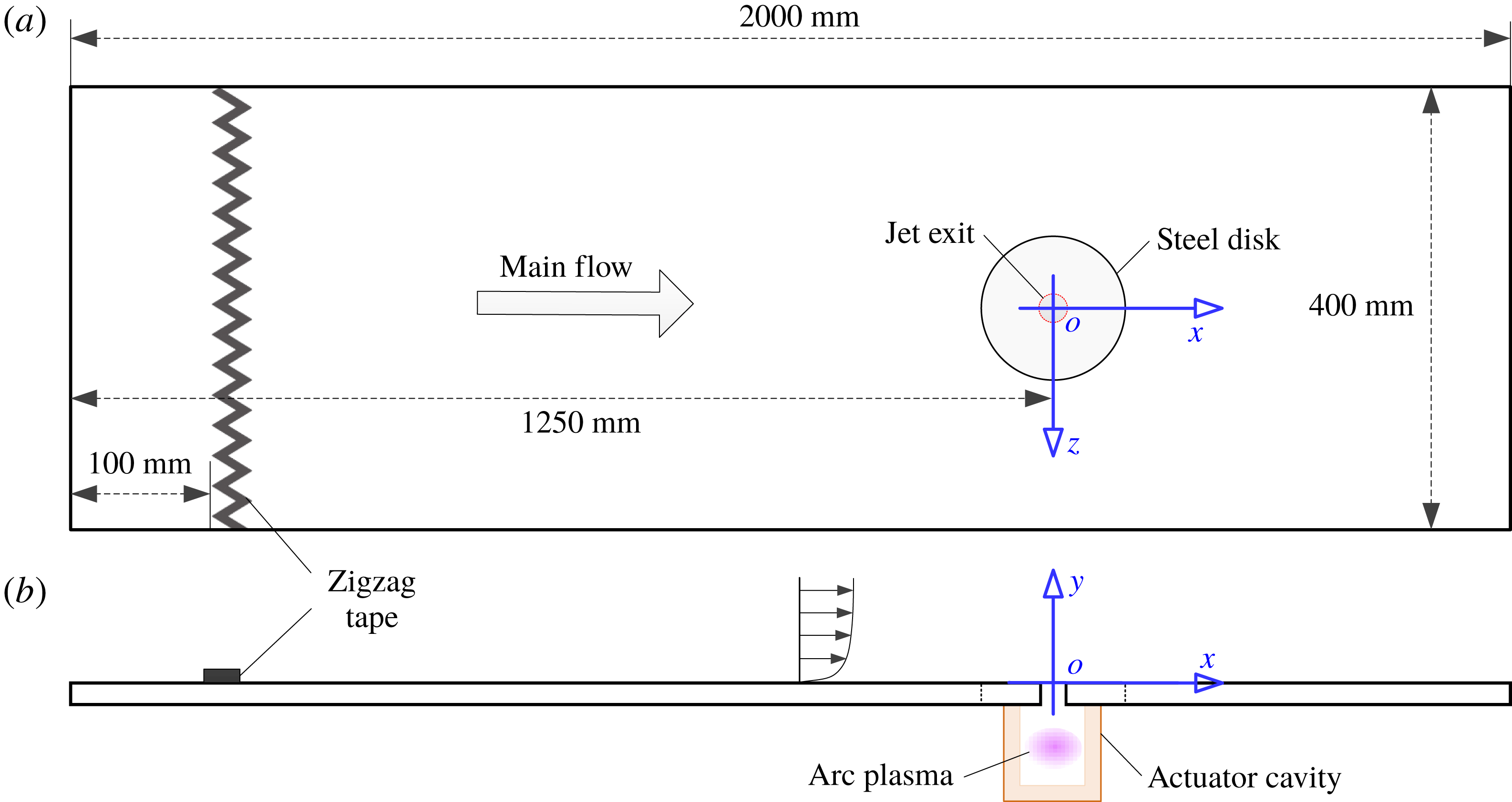
, and the corresponding free-stream turbulence level is approximately 0.5 %. As shown in figure 1, the boundary layer originating from the settling chamber is developed naturally on the bottom plate of this test section and tripped by a zigzag tape located 100 mm downstream of the leading edge. Owing to the growth of the boundary-layer thickness, a slightly favourable pressure gradient is experienced in the test section and estimated to be less than
 $0.024\unicode[STIX]{x1D70C}_{0}U_{\infty }^{2}$
per metre, where
 $\unicode[STIX]{x1D70C}_{0}$
is the ambient density determined by atmospheric pressure (
 $P_{0}=1.01\times 10^{5}~\text{Pa}$
) and temperature (
 $T_{0}=293~\text{K}$
) (Zong & Kotsonis Reference Zong and Kotsonis2017c
). A steel disk is flush-mounted in the bottom plate, and a circular orifice (diameter
 $D=2~\text{mm}$
) is drilled in the centre of this disk, serving as the exit of PSJs. This steel disk accommodates the actuator cavity positioned underneath and provides the possibility of orifice shape investigation. The distance from the exit orifice centre to the leading edge of the bottom plate is 1250 mm. A coordinate system is established in the jet exit centre, with
 $x$
,
 $y$
and
 $z$
being the streamwise direction, wall-normal direction and spanwise direction, respectively.
Bottom plate of the test section: (a) top view and (b) side view. The coordinate system used throughout this study is indicated in blue. Not to scale.

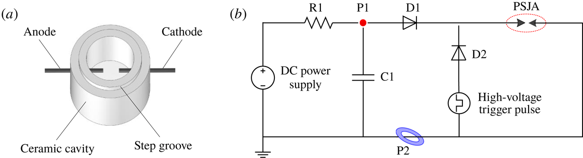
PSJs are issued from an enclosed ceramic cavity directly fitted underneath the steel disk via a circular step groove. The construction of this ceramic cavity (single-walled shell, the material being MACOR) is shown in figure 2(a). The height and diameter of the inner cylindrical cavity are 15 mm and 12 mm, respectively, leading to a cavity volume of
 $V_{ca}=1696~\text{mm}^{3}$
. In a plane located 7.5 mm above the cavity bottom, two opposing holes (diameter 1 mm) are drilled through the cavity wall. Two tungsten needles are inserted through these holes, to act as anode and cathode, respectively. The inter-electrode gap is fixed to 2 mm. The sequential discharge power supply (i.e. a trigger discharge followed by a capacitive discharge) described in Zong & Kotsonis (Reference Zong and Kotsonis2018) is adopted to feed the actuator, as sketched in figure 2(b). The energy-storing capacitor C1 (withstand voltage 5 kV, capacitance
 $0.1~\unicode[STIX]{x03BC}\text{F}$
) is charged by a direct-current (DC) power supply (peak voltage 2.5 kV), with resistor R1 (resistance
 $2~\text{k}\unicode[STIX]{x03A9}$
) limiting the charging current. High-voltage low-current trigger pulses are generated by a high-voltage amplifier (Trek Model 20/20HC) to ignite the electrode gap. As soon as the discharge channel is established, the energy stored in C1 is released rapidly into the electrode gap, thermalizing and pressurizing the cavity gas. Subsequently, C1 is recharged, awaiting for the next trigger pulse. Two diodes (D1 and D2) are added to isolate the high-voltage amplifier and the DC power supply from each other for protection purposes. The intensity and working frequency of the PSJs can be tuned independently by the initial capacitor voltage (
 $V_{0}$
) and trigger frequency (
 $f_{d}$
), respectively.
2.2 Measurement techniques and test scheme
Sketches of (a) actuator cavity and (b) discharge circuit. PSJA is modelled as an air gap in the discharge circuit. P1 and P2 indicate, respectively, the measurement stations of discharge voltage and current.

The primary focus of the present study is the effect of velocity ratio (denoted as
 $r$
) on PSJs in cross-flow. In order to enable variations in velocity ratio, the amplitude of the emitted jet is controlled by appropriate scaling of the discharge energy. This is consequently controlled by the initial capacitor voltage. Four cases with increasing initial capacitor voltage (
 $V_{0}=0.88$
, 1.25, 1.77 and 2.5 kV) are tested. The discharge frequency is fixed at 200 Hz, as this value is slightly lower than the thermal cutoff frequency of a similar geometrical configuration (210 Hz) reported by Zong & Kotsonis (Reference Zong and Kotsonis2017b
). With discharge frequency below this thermal cutoff frequency, the mean cavity density is expected to remain close to the ambient density due to a sufficiently long refresh time.
Electrical measurements are necessary to quantify the discharge energy (
 $E_{d}$
) and duration (
 $T_{d}$
) in each case, which significantly affect the variation of the jet exit velocity (Zong et al.
Reference Zong, Wu, Li, Song, Zhang and Jia2015b
). The discharge voltage (
 $u_{d}$
) and current (
 $i_{d}$
) are measured by a high-voltage probe (Tektronix, P6015A) and a current monitor (Pearson, model 325), respectively; the measurement stations are indicated in figure 2(b). These waveforms are recorded by an oscilloscope (Tektronix, TDS 3054C) at a sampling rate of 1 GHz to compute the discharge energy. Similar to that in Anderson & Knight (Reference Anderson and Knight2012), the discharge energy is normalized by the enthalpy of the cavity gas, resulting in a non-dimensional energy deposition (
 $\unicode[STIX]{x1D716}$
) as shown in (2.1), where
 $c_{p}$
is the constant-pressure specific heat capacity:
 $$\begin{eqnarray}\unicode[STIX]{x1D716}=\frac{E_{d}}{E_{g}}=\frac{\displaystyle \int _{0}^{T_{d}}u_{d}i_{d}\,\text{d}t}{c_{p}\unicode[STIX]{x1D70C}_{0}V_{ca}T_{0}}.\end{eqnarray}$$
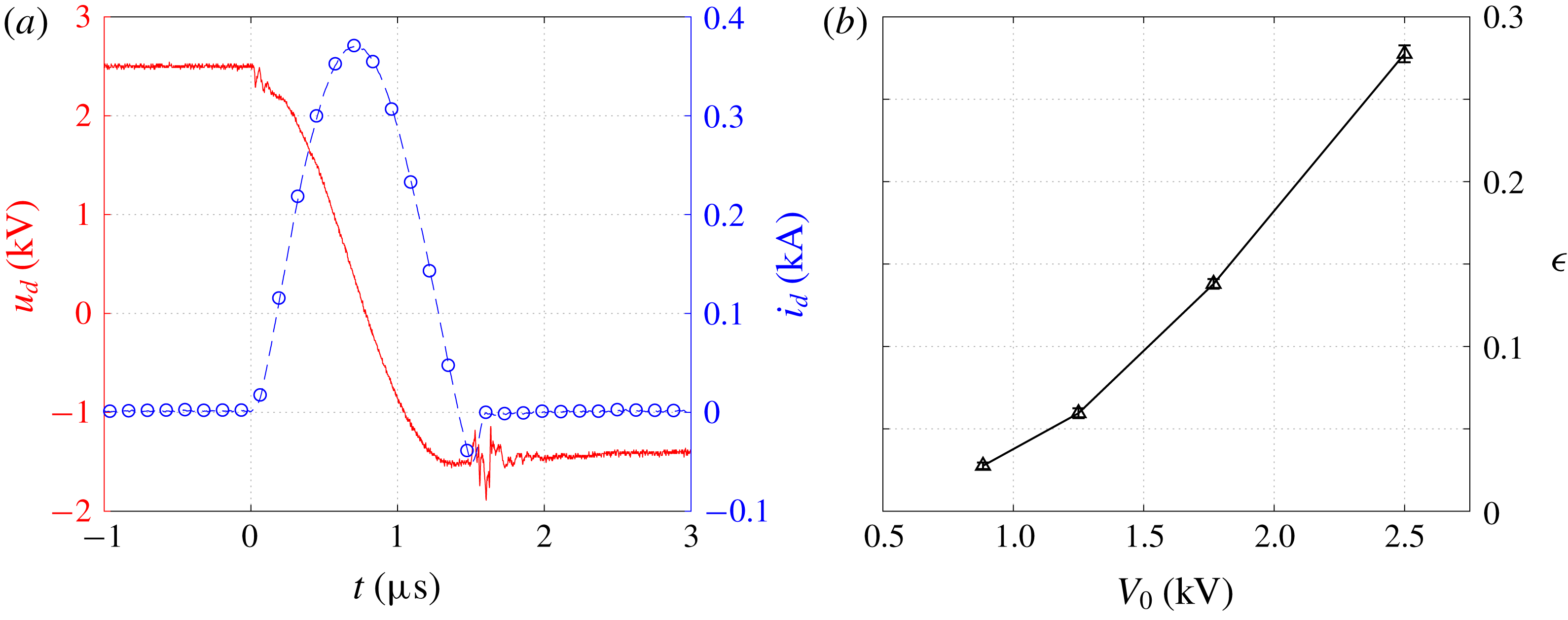
Representative discharge waveforms at
 $V_{0}=2.5~\text{kV}$
are shown in figure 3(a). Immediately after gas breakdown at
 $t=0~\unicode[STIX]{x03BC}\text{s}$
, the capacitor voltage drops steadily, while the discharge current exhibits a half-sine wave. Periodic oscillations, as reported by Belinger et al. (Reference Belinger, Naudé, Cambronne and Caruana2014), are not observed, which is ascribed to the addition of isolation diodes in the discharge circuit (figure 2
b). The discharge duration is estimated to be
 $1.5~\unicode[STIX]{x03BC}\text{s}$
, far less than the characteristic time of jet evolution (Helmholtz natural oscillation period,
 $607~\unicode[STIX]{x03BC}\text{s}$
) (Zong & Kotsonis Reference Zong and Kotsonis2018). The non-dimensional energy deposition (
 $\unicode[STIX]{x1D716}$
) in the four tested cases is shown in figure 3(b);
 $\unicode[STIX]{x1D716}$
ranges from 0.028 to 0.28. Simplified theoretical estimations (Anderson & Knight Reference Anderson and Knight2012; Zong et al.
Reference Zong, Wu, Li, Song, Zhang and Jia2015b
) with a typical electromechanical efficiency of 1 % (Zong & Kotsonis Reference Zong and Kotsonis2016b
) have shown that this range will yield a peak velocity ratio ranging between 1 and 4, which is typically encountered in industrial applications as well as research studies (Mahesh Reference Mahesh2013).
(a) Electrical waveforms measured at an initial capacitor voltage of
 $V_{0}=2.5~\text{kV}$
: —— (red), instantaneous capacitor voltage; – –○– – (blue), instantaneous discharge current. (b) Non-dimensional energy deposition at increasing initial capacitor voltage.

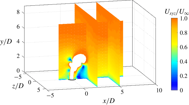
Phase-averaged high-speed PIV measurements are carried out in three wall-normal planes. Of these planes, one is aligned in the streamwise direction (henceforth referenced as the symmetry plane,
 $z/D=0$
), while the remaining two are aligned in the spanwise direction (
 $x/D=2$
and
 $x/D=5$
). As indicated in figure 4, the symmetry-plane measurements aim at the elucidation of the jet trajectory, while the spanwise-plane measurements capture the streamwise vortices. The PIV system mainly consists of two high-speed cameras (Photron, Fastcam SA-1,
 $1024\times 1024$
pixels), a high-speed laser (Quantronix, Darwin Duo 527-80-M) and a programmable timing unit (LaVision, HSC). Depending on the measurement type (planar for the symmetry plane, stereo for the spanwise planes), either one or two cameras are used. On each of the high-speed cameras, a 200 mm objective (Nikon, Micro-Nikkor) fitted with a
 $2\times$
teleconverter (Kenko) is mounted to image a field of view of
 $7.5D\times 7.5D$
and
 $12D\times 12D$
in planar and stereo PIV, respectively. The view angle between the two cameras in stereo configuration is approximately
 $60^{\circ }$
. Scheimpflug adapters are mounted in between cameras and objectives to align the focal plane to the object plane. Laser beams are shaped into a thin sheet (thickness 0.6 mm for planar configuration and 1 mm for stereo), using a combination of two spherical lenses and one cylindrical lens. This laser sheet is kept strictly normal to the bottom plate and transmitted in wall-parallel direction to minimize wall reflection. Liquid particles (mean diameter 1
 $\unicode[STIX]{x03BC}$
m) are seeded in the settling chamber of the wind tunnel by a fog generator (SAFEX, Fog 2010+), using a working fluid of water–glycol mixture. The particle image size is kept as 2–3 pixels to avoid significant peak locking errors (Christensen Reference Christensen2004).
Raw particle images are recorded in phase-locked mode, and the phase (
 $t$
, namely the time delay between discharge ignition and image acquisition) can be adjusted by a digital delay generator (Stanford Research Systems, DG 535). Depending on the peak jet velocity observed in each phase, the time separation between two laser pulses varies between
 $2~\unicode[STIX]{x03BC}\text{s}$
and
 $8~\unicode[STIX]{x03BC}\text{s}$
to guarantee a peak particle displacement of approximately 10 pixels. For each of the four tested cases, 54 phases are selected in one cycle to retrieve the entire evolution of PSJs in cross-flow, ranging from the emanation of incipient jets to the termination of the suction stage. For each of the 54 phases, 300 image pairs are recorded to arrive at statistically converged velocity fields. Both image acquisition and post-processing are implemented by LaVision Davis 8.3.1. In the final pass of cross-correlation operation, the interrogation window size and the overlapping ratio are
 $16\times 16$
and 75 %, respectively, leading to a spatial resolution of
 $0.07~\text{mm}~\text{vector}^{-1}$
and
 $0.1~\text{mm}~\text{vector}^{-1}$
in planar and stereo PIV measurements. In addition to measurements under PSJs in cross-flow conditions, the baseline unactuated boundary layer and the PSJs without cross-flow boundary layer (quiescent flow) are also measured. In the case of baseline boundary layer test, 2000 samples are acquired at 2 kHz at each of the three measurement planes to get converged mean flow quantities as well as Reynolds stresses. The field of view in the symmetry plane (
 $z/D=0$
) is enlarged to
 $15D\times 15D$
to cover the entire boundary layer. For PSJs in quiescent flow, similar phase-averaged measurements as mentioned earlier are performed, whereas only 100 samples are acquired at each phase.
Fields of view in two-component planar and three-component stereo PIV measurements. The magnitude of total velocity (
 $U_{xyz}$
) at a time delay of
 $t=300~\unicode[STIX]{x03BC}\text{s}$
with regard to discharge ignition is displayed as contours. High-velocity regions (
 $U_{xyz}/U_{\infty }\geqslant 1$
) are cropped to visualize the bending jet.

Peak locking error, finite sample size, finite laser sheet thickness and discharge timing uncertainty are identified as the four main sources of phase-averaged PIV measurement uncertainty. Following a similar procedure as that in Zong & Kotsonis (Reference Zong and Kotsonis2017a
,Reference Zong and Kotsonis
c
), each of the four measurement uncertainties can be estimated a posteriori. The total measurement error is defined as the Euclidean sum (i.e. root-sum-square) of these four uncertainties (Sciacchitano & Wieneke Reference Sciacchitano and Wieneke2016). As a result, the peak errors for streamwise and wall-normal velocity components in planar PIV measurements are estimated to be 2.4 % and 4.9 % of the peak jet velocity. In stereo PIV measurements, the camera view angle is taken into account during the estimation of peak locking error, and the peak uncertainties pertaining to the three velocity components (i.e.
 $U_{x}$
,
 $U_{y}$
and
 $U_{z}$
) are computed to be 6.0 %, 3.0 % and 3.5 % of
 $U_{\infty }$
, respectively.
3 Baseline results
3.1 Symbol convention
Prior to introducing any results, symbol notation is defined. The instantaneous, phase-averaged and time-averaged velocity are denoted, respectively, by
 $u$
,
 $U$
and
 $\bar{U}$
. Reynolds & Hussain (Reference Reynolds and Hussain1972) proposed a triple decomposition of the instantaneous velocity, as shown below:
 $$\begin{eqnarray}u(x,y,z,t)=\bar{U}(x,y,z)+\tilde{u} (x,y,z,t)+u^{\prime }(x,y,z,t),\end{eqnarray}$$
where
 $\bar{U}$
,
 $\tilde{u}$
and
 $u^{\prime }$
represent, respectively, the time-invariant contribution, the periodic fluctuation arising from repetitive actuation and the random fluctuation corresponding to turbulence. The summation of time-invariant and periodic-fluctuation parts yields the phase-averaged velocity (
 $U$
). The time-averaged velocity is essentially the integral of the phase-averaged velocity in one cycle period (denoted as
 $T_{d}$
) and can be approximated by a weighted summation as indicated in (3.2), where
 $\unicode[STIX]{x0394}t$
is the time step between successive phases:
 $$\begin{eqnarray}\displaystyle \bar{U}(x,y,z)=\int _{0}^{T_{d}}U(x,y,z,t)\,\text{d}t\approx \frac{1}{T_{d}}\mathop{\sum }_{i=1}^{N}U_{i}(x,y,z,t)\,\unicode[STIX]{x0394}t_{i}. & & \displaystyle\end{eqnarray}$$
We denote by
 $\unicode[STIX]{x1D70F}_{w}$
and
 $\unicode[STIX]{x1D6FF}_{99}$
the wall shear stress and the boundary thickness determined by
 $99\,\%\,U_{\infty }$
, respectively; and
 $\unicode[STIX]{x1D6FF}^{\ast }$
and
 $\unicode[STIX]{x1D703}$
are the displacement thickness and the momentum thickness of the boundary layer defined by (3.3) and (3.4), where
 $\bar{U}_{x,min}$
is the minimum velocity in the profile (Dandois, Garnier & Sagaut Reference Dandois, Garnier and Sagaut2007):
 $$\begin{eqnarray}\displaystyle & \displaystyle \unicode[STIX]{x1D6FF}^{\ast }=\int _{0}^{\unicode[STIX]{x1D6FF}_{99}}\left(1-\frac{\bar{U}_{x}-\bar{U}_{x,min}}{U_{\infty }-\bar{U}_{x,min}}\right)\text{d}y, & \displaystyle\end{eqnarray}$$
 $$\begin{eqnarray}\displaystyle & \displaystyle \unicode[STIX]{x1D703}=\int _{0}^{\unicode[STIX]{x1D6FF}_{99}}\frac{\bar{U}_{x}-\bar{U}_{x,min}}{U_{\infty }-\bar{U}_{x,min}}\left(1-\frac{\bar{U}_{x}-\bar{U}_{x,min}}{U_{\infty }-\bar{U}_{x,min}}\right)\text{d}y. & \displaystyle\end{eqnarray}$$
The ratio of the displacement thickness to momentum thickness defines the boundary-layer shape factor,
 $H=\unicode[STIX]{x1D6FF}^{\ast }/\unicode[STIX]{x1D703}$
. When no reverse flow occurs (
 $\bar{U}_{x,min}=0~\text{m}~\text{s}^{-1}$
), these definitions collapse to the orthodox definitions in Schlichting & Gersten (Reference Schlichting and Gersten2017). However, in the case of strong reverse flow, these definitions can effectively suppress the rise of the shape factor. Finally,
 $u_{\unicode[STIX]{x1D70F}}$
and
 $\unicode[STIX]{x1D6FF}_{v}$
denote the viscous velocity and length scale, respectively; and
 $y^{+}$
and
 $u^{+}$
are defined as
 $y^{+}=\bar{U}_{x}/u_{\unicode[STIX]{x1D70F}}$
and
 $u^{+}=y/\unicode[STIX]{x1D6FF}_{v}$
, respectively.
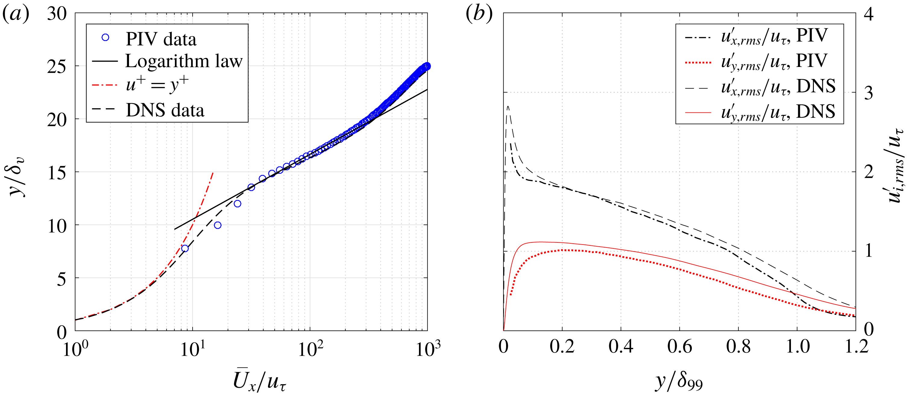
3.2 Unactuated turbulent boundary layer
(a) Mean velocity profiles and (b) Reynolds normal stresses measured at
 $x/D=2$
and
 $z/D=0$
. DNS data from Wu et al. (Reference Wu, Moin, Wallace, Skarda, Lozano-Durán and Hickey2017) at
 $Re_{\unicode[STIX]{x1D703}}=2900$
are compared.

The mean velocity profile and the root-mean-square of the turbulent velocity fluctuation (denoted as
 $u_{i,rms}^{\prime }$
) measured in the symmetry plane at
 $x/D=2$
are shown in figure 5. As a result,
 $\unicode[STIX]{x1D6FF}_{99}$
,
 $\unicode[STIX]{x1D6FF}^{\ast }$
and
 $\unicode[STIX]{x1D703}$
are computed to be 19.3 mm, 3.2 mm and 2.3 mm, respectively. The boundary-layer shape factor is 1.36 and changes marginally in the measurement domain, indicating a fully developed turbulent boundary layer. The Reynolds number based on the momentum thickness and free-stream velocity (
 $Re_{\unicode[STIX]{x1D703}}$
) is approximately 3000. In the inertial range (
 $0.03\leqslant y/\unicode[STIX]{x1D6FF}_{99}\leqslant 0.3$
) of the turbulent boundary layer, the variation of mean velocity follows a logarithmic law (Schlichting & Gersten Reference Schlichting and Gersten2017), as shown in (3.5), where
 $\unicode[STIX]{x1D705}$
is the von Kármán constant (0.40):
 $$\begin{eqnarray}\frac{\bar{U}_{x}}{u_{\unicode[STIX]{x1D70F}}}=\frac{1}{\unicode[STIX]{x1D705}}\ln \frac{y}{\unicode[STIX]{x1D6FF}_{v}}+b.\end{eqnarray}$$
Based on this relation and the measured velocity profile,
 $u_{\unicode[STIX]{x1D70F}}$
and
 $\unicode[STIX]{x1D6FF}_{v}$
are determined to be
 $0.80~\text{m}~\text{s}^{-1}$
and
 $19.1~\unicode[STIX]{x03BC}\text{m}$
, respectively. Direct numerical simulation (DNS) data from Wu et al. (Reference Wu, Moin, Wallace, Skarda, Lozano-Durán and Hickey2017) at a similar momentum-thickness-based Reynolds number (
 $Re_{\unicode[STIX]{x1D703}}=2900$
) are plotted for comparison. As a result, the mean velocity profile collapses well even in the buffer layer (
 $8\leqslant y^{+}\leqslant 30$
). The turbulent velocity fluctuations (figure 5
b) from DNS are slightly higher than from PIV in the near-wall region (
 $y/\unicode[STIX]{x1D6FF}_{99}\leqslant 0.1$
) and decay relatively slowly in the outer boundary layer (
 $y/\unicode[STIX]{x1D6FF}_{99}\geqslant 0.8$
), further confirming the reliability and accuracy of the present PIV measurements.
3.3 Plasma synthetic jets in quiescent flow
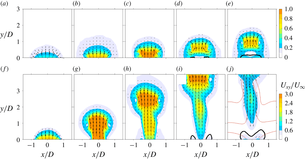
Phase-averaged velocity fields in case 1 (a–e,
 $\unicode[STIX]{x1D716}=0.028$
) and case 4 (f–j,
 $\unicode[STIX]{x1D716}=0.28$
). The dimensionless convective time is identical in each row and increases linearly from
 $t^{\ast }=1$
to
 $t^{\ast }=5$
in a step of 1 time unit (a–j). Direction and magnitude of the in-plane velocity (
 $U_{xy}$
) are displayed as contours and vectors. The thick black lines near the jet exit are contour lines of
 $U_{y}/U_{\infty }=-0.1$
. The thin red lines in panel (j) are streamlines.

The time evolution of the phase-averaged velocity fields in case 1 (
 $\unicode[STIX]{x1D716}=0.028$
) and case 4 (
 $\unicode[STIX]{x1D716}=0.28$
) is shown in figure 6. Although no external flow is present, the free-stream velocity pertaining to the flow cases (
 $U_{\infty }$
) and the exit orifice diameter (
 $D$
) are used to normalize time and facilitate comparison, resulting in a dimensionless convection time,
 $t^{\ast }=tU_{\infty }/D$
. In both cases, a vortex ring is shed from the exit orifice as a result of an abrupt expansion of the cavity gas immediately after the pulsed arc discharge. This vortex ring propagates along the axisymmetry axis of the actuator throat and entrains the surrounding fluids into its core region, leading to growing size. This core region exhibits the highest velocity as a result of the self-induction effect of vortex rings. Suction flow, as visualized by the contour lines of
 $U_{y}/U_{\infty }=-0.1$
, is initialized at the periphery of the jet exit at
 $t^{\ast }=4$
. An inward growth of the suction region is experienced afterwards, and the entire orifice is occupied at
 $t=5^{\ast }$
. The general topology of the emanating jets agrees well with results of past characterization studies (Zong & Kotsonis Reference Zong and Kotsonis2017b
, Reference Zong and Kotsonis2018).
The leading vortex ring in case 4 is initially connected with a trailing jet (
 $t^{\ast }=2$
) which severs from the jet front after
 $t^{\ast }=5$
. As a comparison, the vortex ring in case 1 is always isolated during evolution. This morphological difference is attributed to the ‘formation number’ of vortex rings, which is reported to be 3.6–4.5 by Gharib et al. (Reference Gharib, Rambod and Shariff1998) and Sau & Mahesh (Reference Sau and Mahesh2007). Note that the ‘formation number’ of vortex rings is an inherently different concept than the formation threshold of conventional synthetic jets proposed by Holman et al. (Reference Holman, Utturkar, Mittal, Smith and Cattafesta2005). Specifically, when the stroke ratio
 $L_{s}^{\ast }$
defined by
 $$\begin{eqnarray}L_{s}^{\ast }=\frac{L_{s}}{D}=\frac{1}{\unicode[STIX]{x1D70C}_{0}D}\int _{0}^{T_{jet}}\unicode[STIX]{x1D70C}_{e}(t)U_{ey}(t)\,\text{d}t\end{eqnarray}$$
(Glezer & Amitay Reference Glezer and Amitay2002; Zong & Kotsonis Reference Zong and Kotsonis2018) is below the formation number, the vorticity shed from the jet exit will be absorbed completely by the vortex ring, and no trailing jet column will form. In contrast, the formation threshold of synthetic jets (
 $L_{s}^{\ast }>0.5$
for a round orifice) only guarantees that the vortex ring created in the ejection phase will not be drawn back into the actuator cavity during the subsequent ingestion phase (Holman et al.
Reference Holman, Utturkar, Mittal, Smith and Cattafesta2005).
In the above definition,
 $T_{jet}$
is the duration of the ejection stroke;
 $\unicode[STIX]{x1D70C}_{e}$
and
 $U_{ey}$
are the spatially averaged jet exit density and jet exit velocity, respectively. In the case of axisymmetric jets, the following relation can be derived straightforwardly:
 $$\begin{eqnarray}U_{ey}=\frac{4}{D^{2}}\int _{-D/2}^{D/2}xU_{y}(x,t)|_{y=0}\,\text{d}x.\end{eqnarray}$$
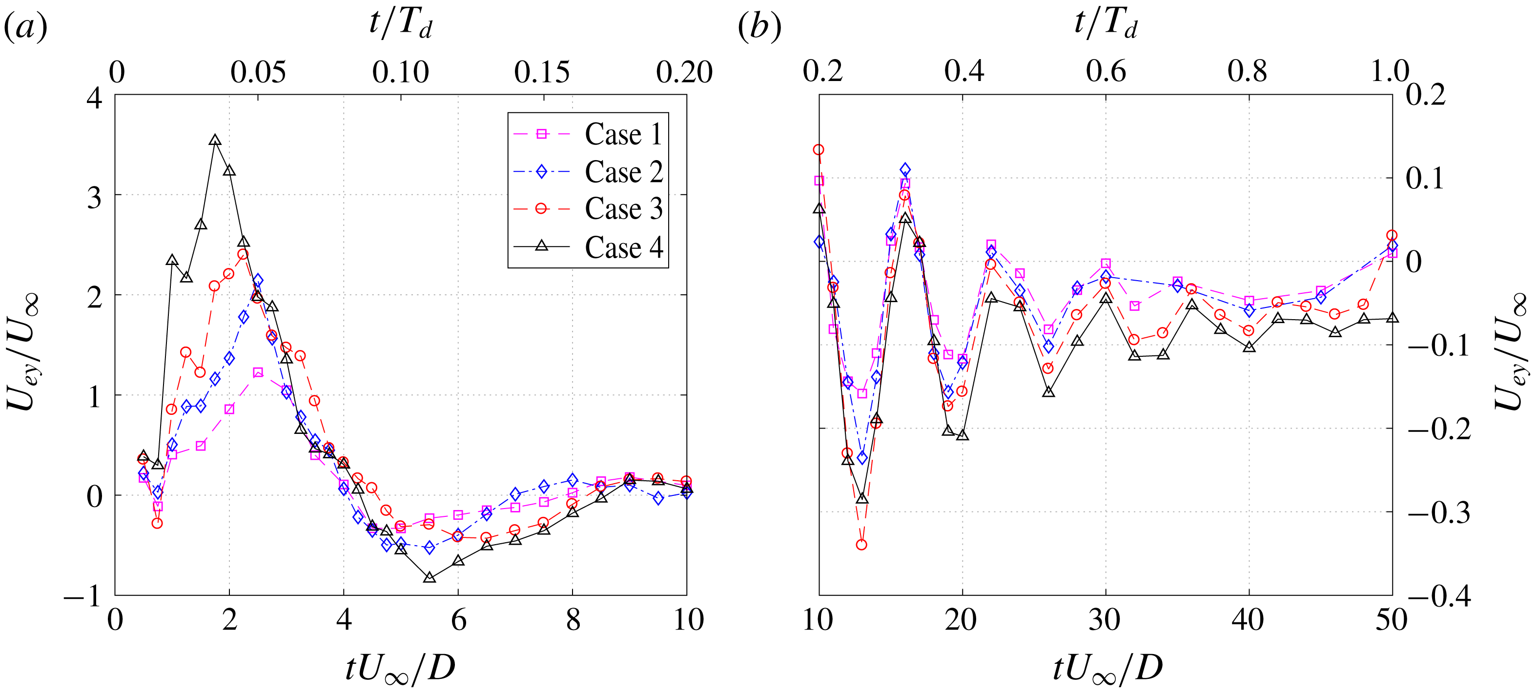
The variation of
 $U_{ey}$
with one actuation cycle is extracted from PIV results and shown in figure 7. For all the cases, a prominent jet stage is perceived immediately after discharge ignition, where
 $U_{ey}$
first rises and then decays. As energy deposition (
 $\unicode[STIX]{x1D716}$
) increases, the peak jet exit velocity (
 $U_{p}$
) increases monotonically from
 $1.2U_{\infty }$
to
 $3.5U_{\infty }$
, whereas the duration of the primary jet stage (
 $T_{jet}$
) changes marginally (400–
 $450~\unicode[STIX]{x03BC}\text{s}$
). Periodic oscillations pivoting around
 $U_{ey}/U_{\infty }=-0.1$
with decaying amplitude are noticed in the later evolution of
 $U_{ey}$
(
 $t^{\ast }>5$
), pertaining to the occurrence of weak suction flow. Based on the amount of velocity peaks within one period, the oscillation frequency is determined to be 1.6 kHz, which reconciles well with the estimated Helmholtz natural resonance frequency of the present PSJA cavity (
 $f_{h}=1.65$
kHz) (Chiatto & de Luca Reference Chiatto and de Luca2017; Zong & Kotsonis Reference Zong and Kotsonis2018). The Helmholtz natural resonance frequency is derived from the stiffness of the cavity gas and mainly affected by geometrical and atmospheric parameters as shown in (3.8), where
 $\unicode[STIX]{x1D6FE}$
and
 $A_{e}$
are the specific heat ratio and the area of the exit orifice, respectively:
 $$\begin{eqnarray}f_{h}=\frac{1}{2\unicode[STIX]{x03C0}}\sqrt{\frac{\unicode[STIX]{x1D6FE}P_{0}}{\unicode[STIX]{x1D70C}_{0}}}\sqrt{\frac{A_{e}}{V_{ca}L_{th}}}.\end{eqnarray}$$
Evolution of the spatially averaged exit velocity (
 $U_{ey}$
) in one period for all the tested cases. Scales of
 $y$
-axis are changed to adapt for the different velocity range.

For conventional SJAs driven by vibrating diaphragms, the frequency response of the peak exit velocity exhibits a maximum at
 $f_{h}$
(Gallas et al.
Reference Gallas, Carroll, Cattafesta, Holman, Nishida and Sheplak2003; de Luca, Girfoglio & Coppola Reference de Luca, Girfoglio and Coppola2014), i.e. operating at this frequency is beneficial. Nevertheless, for PSJAs,
 $f_{h}$
is generally interpreted as the theoretical limit working frequency above which significant misfires are expected due to a shortage of refresh time (Narayanaswamy et al.
Reference Narayanaswamy, Raja and Clemens2010; Zong & Kotsonis Reference Zong and Kotsonis2017b
). In this study, the discharge frequency (
 $f_{d}=200$
Hz) is approximately
 $0.12f_{h}$
, and no significant frequency effect (e.g. reduced jet density, increasing cavity temperature) is expected.
The manifestation of the Helmholtz natural frequency in figure 7 can also be explained from a theoretical perspective. Specifically, the formation process of PSJs is essentially the time response of a fluid system (a cavity with an opening, i.e. Helmholtz resonator) to a localized heat disturbance (Chiatto et al.
Reference Chiatto, Capuano, Coppola and de Luca2017). Since this heat disturbance (arc discharge) is imposed abruptly within
 $0.2\,\%\,T_{h}$
, the solution collapses to the impulse response of this fluid system described by the second-order Navier–Stokes equation. This is somehow reasonable, as the curves in figure 3.7 do resemble the impulse response of a second-order underdamped system. As such, the inherent resonance frequency of this fluid system will be excited and manifested in the time response.
Based on these exit-velocity curves, the time-mean jet exit density in the ejection stroke (
 $\bar{\unicode[STIX]{x1D70C}}_{e}$
) can be estimated using the mass conservation law (Zong & Kotsonis Reference Zong and Kotsonis2018). As a result,
 $\bar{\unicode[STIX]{x1D70C}}_{e}/\unicode[STIX]{x1D70C}_{0}$
varies from 0.9 to 0.8 with increasing energy deposition, and the total expelled gas mass in the jet stages is less than 2 % of the initial cavity mass (
 $\unicode[STIX]{x1D70C}_{0}V_{c}a$
). This noticeable density variation indicates non-negligible compressibility effects, which once again differentiate PSJs from the conventional piezoelectric synthetic jets. Additionally, based on (3.6), the stroke ratio for the four tested cases is computed to vary from 2.0 to 5.4 (see table 1). This justifies the earlier interpretation of figure 6 based on the formation number of vortex rings (3.6).
The time-mean velocity in the ejection stroke (
 $U_{0}=L_{s}/T_{jet}$
) is selected as the reference velocity to compute the jet Reynolds number (
 $Re_{D}=U_{0}D/\unicode[STIX]{x1D708}$
) and the velocity ratio (
 $r=U_{0}/U_{\infty }$
) (Smith & Glezer Reference Smith and Glezer1998). The Strouhal number is based on orifice diameter and free-stream velocity,
 $St=f_{d}D/U_{\infty }$
, consistent with Jabbal & Zhong (Reference Jabbal and Zhong2008). These parameters (
 $L_{s}^{\ast },Re_{D},r,St$
), plus the skin friction coefficient (
 $c_{f}=\unicode[STIX]{x1D70F}_{w}/0.5\unicode[STIX]{x1D70C}_{0}U_{\infty }^{2}$
), and the ratio of boundary-layer thickness to orifice diameter (
 $h=\unicode[STIX]{x1D6FF}_{99}/D$
), constitute the six dimensionless quantities that govern the pertinent physics of PSJs in cross-flow, as listed in table 1. The free-stream Reynolds number based on boundary-layer thickness is not included due to the following interdependence:
 $Re_{\unicode[STIX]{x1D6FF}}=Re_{L}h/(rL_{s}^{\ast })$
. In contrast with conventional synthetic jets driven by oscillating diaphragms (Jabbal & Zhong Reference Jabbal and Zhong2008), the Strouhal number is included in the parameter space of PSJs, since
 $St=0.5r/L_{s}^{\ast }$
no longer holds. Of all these parameters, stroke length and velocity ratio play a dominant role in the flow field evolution (Sau & Mahesh Reference Sau and Mahesh2008; Jabbal & Zhong Reference Jabbal and Zhong2010). Since the jet duration time is fixed by the actuator geometry in this study, the effects of
 $r$
and
 $L_{s}^{\ast }$
are effectively combined, i.e. high jet velocity always indicates large stroke length.
Jet formation parameters for all the tested cases.

4 Plasma synthetic jets in cross-flow at
 $r=1.6$

This section focuses on case 4 (
 $r=1.6$
), which, based on the quiescent measurements, is characterized by the highest formation number
 $(L_{s}/D=5.4)$
among the tested cases. Phase-averaged velocity fields in the symmetry plane are first introduced, and effects of several pertinent flow features (shock waves, vortex rings, back-flow, suction flow) on the boundary layer are analysed in detail. Subsequently, streamwise vortices are identified in the spanwise measurement planes (
 $yz$
-planes), and the interconnections between these streamwise vortices and the flow features in the symmetry plane are interpreted to establish a clear picture of PSJs in cross-flow at high velocity ratio and large stroke length.
4.1 Symmetry plane
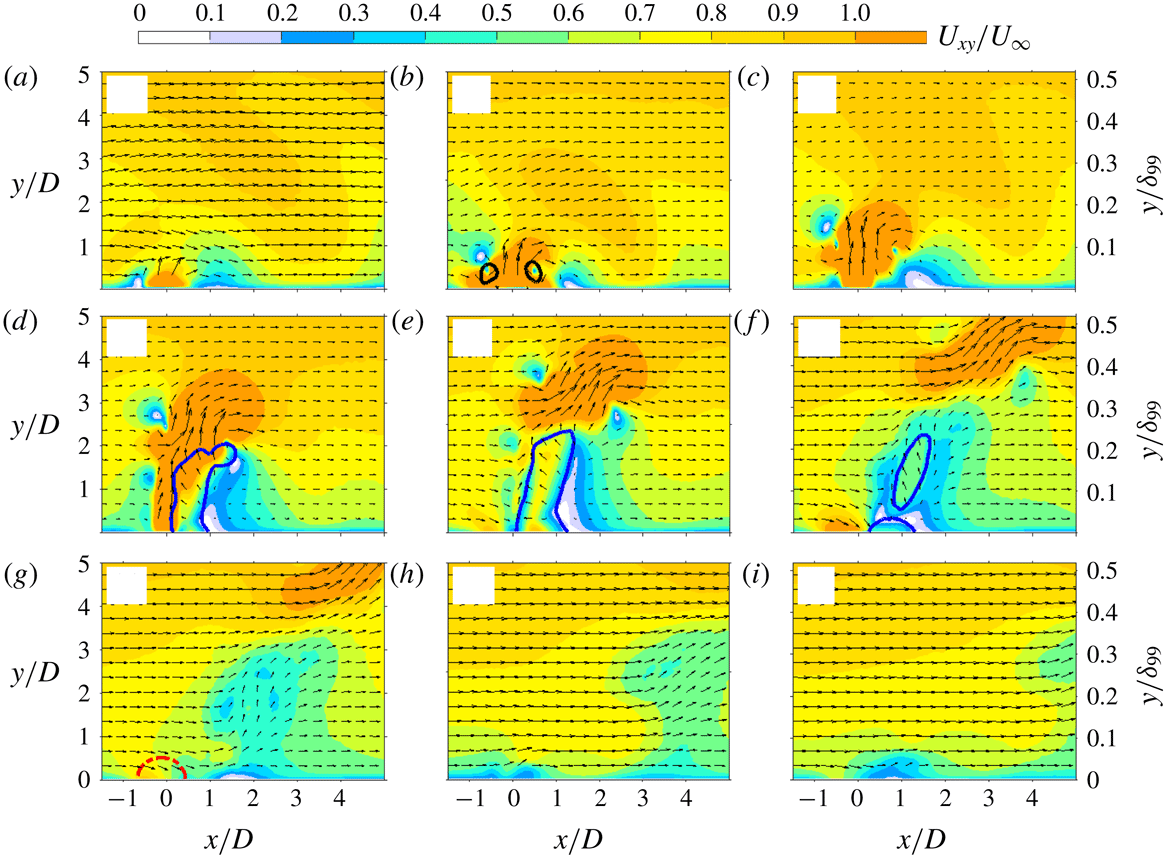
Phase-averaged velocity fields in case 4 (
 $r=1.6$
): (a)
 $t^{\ast }=1$
; (b)
 $t^{\ast }=1.5$
; (c)
 $t^{\ast }=2.0$
; (d)
 $t^{\ast }=3$
; (e)
 $t^{\ast }=4$
; (f)
 $t^{\ast }=5.5$
; (g)
 $t^{\ast }=7$
; (h)
 $t^{\ast }=10$
; (i)
 $t^{\ast }=12$
. The magnitude and direction of the in-plane velocity (
 $U_{xy}$
) are displayed as contours and vectors. The black lines in panel (b) indicate the front vortex ring detected with a criterion of 10 % of the peak
 $Q$
-value. The blue lines in panels (d–f) are contour lines of
 $U_{x}/U_{\infty }=-0.1$
. The red dash-dotted lines in panel (g) are contour lines of
 $U_{y}/U_{\infty }=-0.2$
.

The time evolution of the phase-averaged velocity fields in the symmetry plane (
 $z=0$
mm) is shown in figure 8, where
 $U_{xy}$
denotes the Euclidean norm of the in-plane velocity vector, i.e.
 $U_{xy}=(U_{x}^{2}+U_{y}^{2})^{0.5}$
. Since the peak jet velocity is much higher than the free-stream velocity in this case (
 $U_{p}/U_{\infty }=3.5$
), the jet body can be roughly represented by the region with
 $U_{xy}/U_{\infty }>1$
. An incipient jet manifested in a bump shape is observed at
 $t^{\ast }=1$
. The vorticity residing in the periphery of this incipient jet rolls into a vortex ring (
 $t^{\ast }=1.5$
), and propagation of this vortex ring is followed by a high-speed trailing jet column (
 $t^{\ast }=2$
), similar to the case of quiescent flow. This jet column is initially upright, whereas it bends in relation to the cross-flow during later evolution (
 $t^{\ast }=3$
), as a result of the streamwise pressure difference across the jet orifice (Muppidi & Mahesh Reference Muppidi and Mahesh2005). Concurrently, the flow in the windward side is stagnated, creating a high-pressure zone; whereas a back-flow region associated with a HVP is generated in the leeward side of the jet column (Meyer, Pedersen & Özcan Reference Meyer, Pedersen and Özcan2007), analogous to the recirculation region in cylinder flow and producing a low-pressure core. The back-flow diminishes in area after the jet terminates (
 $t^{\ast }\geqslant 4$
) and leaves a significant momentum deficit in the symmetry plane. Additionally, a weak suction region and a low-speed ejection can be perceived near the exit orifice during later evolution (
 $7\leqslant t^{\ast }\leqslant 12$
).
At
 $t^{\ast }=1$
, the velocity contour lines in the outer boundary layer (
 $y/\unicode[STIX]{x1D6FF}_{99}>0.3$
) manifest a noticeable undulation, which seems peculiar as the incipient jet is still embedded within
 $y/\unicode[STIX]{x1D6FF}_{99}<0.1$
. To further gauge this effect, contours of
 $U_{y}$
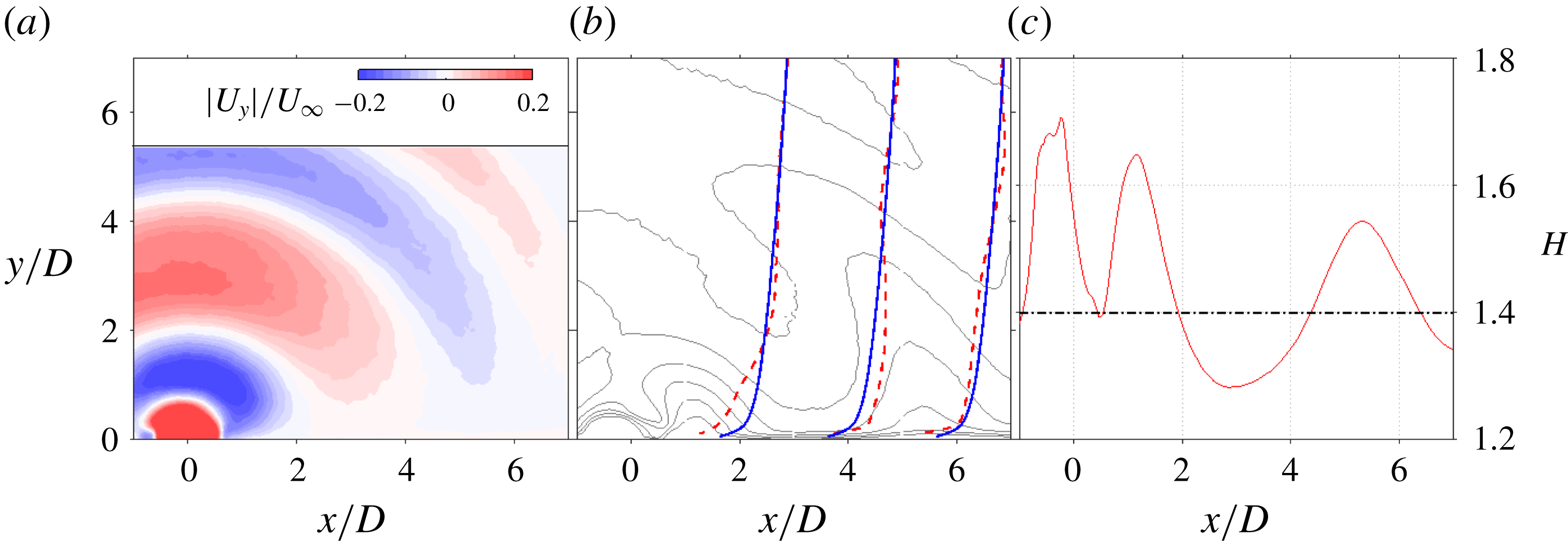
, the boundary-layer velocity profiles as well as the shape factor are shown in figure 9. As evidenced, multiple compression/expansion waves at a wall-normal spacing of approximately
 $2D$
are issued from the exit orifice. These waves are generated from the non-uniform heating of the pulsed arc discharge, and their locations are synchronized by the discharge ignition within an uncertainty of approximately
 $1~\unicode[STIX]{x03BC}\text{s}$
(Laurendeau et al.
Reference Laurendeau, Léon, Chedevergne, Senoner and Casalis2017). Periodic alternations of outward and inward disturbance velocity of the order of several metres per second are induced by these propagating waves (Zong & Kotsonis Reference Zong and Kotsonis2016a
). This disturbance velocity is superimposed on the existing boundary-layer velocity profile, leading to a valley-shaped velocity contour line and a corresponding undulation of the boundary-layer shape factor. Specifically, at the time instant
 $t^{\ast }=1$
, the superposition of compression wavefronts on the boundary layer leads to a fuller velocity profile between
 $2<x/D<4$
, whereas the regions influenced by expansion wavefronts are decelerated.
(a) Contour of wall-normal velocity (
 $U_{y}$
) at
 $t^{\ast }=1$
for case 4. (b) Boundary-layer velocity profiles at
 $t^{\ast }=1$
and
 $x/D=1$
, 3, 5 (red dashed lines). The velocity profiles of the unactuated boundary layer are indicated by solid blue lines. The thin dark lines superimposed on the background are contour lines of streamwise velocity ranging from
 $U_{x}/U_{\infty }=1.0$
(top) to
 $U_{x}/U_{\infty }=0.4$
(bottom) in steps of
 $-0.1$
. (c) Streamwise variation of the boundary-layer shape factor (
 $H$
) at
 $t^{\ast }=1$
. The baseline value (1.4) is indicated as a thick black line for comparison.

Time evolution of vorticity contour in case 4 (
 $r=1.6$
): (a)
 $t^{\ast }=1.5$
; (b)
 $t^{\ast }=2.0$
; (c)
 $t^{\ast }=3$
; (d)
 $t^{\ast }=4$
. Vortices indicated by the black lines are detected with a criterion of 10 % of the peak
 $Q$
-value. The blue dashed lines are contour lines of
 $U_{x}/U_{\infty }=-0.1$
. The red solid lines are streamlines that originate from the centre of the exit orifice.

The time evolution of the vorticity field between
 $t^{\ast }=1.5$
and
 $t^{\ast }=4$
is shown in figure 10. Vortices are identified with the
 $Q$
-criterion using a threshold of 10 % of the peak
 $Q$
-value to filter trivial vortex filaments (Chakraborty, Balachandar & Adrian Reference Chakraborty, Balachandar and Adrian2005). Spanwise vorticity (
 $\unicode[STIX]{x1D714}_{z}$
) is normalized by
 $rU_{\infty }/D$
. High vorticity resides in the front vortex ring (FVR) and jet shear layer. The diameter of the FVR expands as a result of entrainment, and the axis of the vortex ring tilts downstream after
 $t^{\ast }\geqslant 3$
. This downstream tilting is an unstable process, related to the uneven momentum injection received by the two sides of the FVR (Zong & Kotsonis Reference Zong and Kotsonis2016a
). Specifically, as the FVR penetrates higher into the turbulent boundary layer, it experiences a higher convection velocity than the base of the trailing jet, which causes a misalignment of the FVR axis with respect to the trailing jet column (
 $t^{\ast }=2$
). This misalignment brings more momentum from the high-speed trailing jet to the upstream side of the ring, whereas it partially cuts off the momentum injection to the downstream side. As a result, the two sides exhibit a different propagation velocity, and the FVR tilts downstream. This developing downstream tilting pinches off the connection of the FVR with the trailing jet column and creates a kink point in the middle streamline. In the windward side of this kink point, SVs are identified. In the leeward side of the jet body, the negative vorticity diminishes after
 $t^{\ast }=4$
due to the upstream growth of back-flow. These observations are consistent with the DNS results of pulsed jets in laminar cross-flow (Sau & Mahesh Reference Sau and Mahesh2008).
Circulation (
 $\unicode[STIX]{x1D6E4}$
) and centre location (
 $x_{v},y_{v}$
) of the two sides of the FVR can be computed with (4.1)–(4.3), where the integral is limited to the vortex region identified in figure 10:
 $$\begin{eqnarray}\displaystyle & \displaystyle \unicode[STIX]{x1D6E4}^{+}=\iint \unicode[STIX]{x1D714}_{z}^{+}\,\text{d}x\,\text{d}y, & \displaystyle\end{eqnarray}$$
 $$\begin{eqnarray}\displaystyle & \displaystyle x_{v}^{+}=\frac{1}{\unicode[STIX]{x1D6E4}^{+}}\iint x\unicode[STIX]{x1D714}_{z}^{+}\,\text{d}x\,\text{d}y, & \displaystyle\end{eqnarray}$$
 $$\begin{eqnarray}\displaystyle & \displaystyle y_{v}^{+}=\frac{1}{\unicode[STIX]{x1D6E4}^{+}}\iint y\unicode[STIX]{x1D714}_{z}^{+}\,\text{d}x\,\text{d}y. & \displaystyle\end{eqnarray}$$
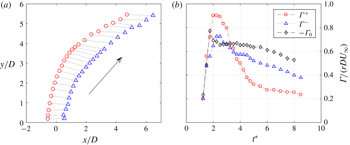
Superscripts (+ or -) are added to distinguish the upstream side from the downstream side. Figure 11 shows the trajectory of the FVR. It is evident that the downstream tilting of the ring reaches a maximum between
 $3<y/D<4$
, and a gradual recovery to wall-normal orientation is exhibited afterwards. This recovery is caused by Kutta–Joukowski lift, which dominates the motion of isolated vortex rings in cross-flow. In this situation, the upstream side experiences a downward lift force, whereas the downstream side undergoes an upward force (Sau & Mahesh Reference Sau and Mahesh2008). This natural tendency to tilt upstream is initially inhibited by the presence of the trailing jet column and finally manifested after the pinch-off. In figure 11(b), the dimensionless vortex ring circulation (
 $\unicode[STIX]{x1D6E4}/rDU_{\infty }$
) in both cross-flow and quiescent conditions is plotted against time (
 $s$
). A non-monotonic variation is exhibited by these curves, and the peak circulations are close to each other (0.7–0.9). In the later evolution (
 $t^{\ast }>3$
), a faster dissipation rate of circulation is exhibited in cross-flow, which can be ascribed to the higher entrainment rate of vortex rings in cross-flow (Sau & Mahesh Reference Sau and Mahesh2008). Additionally,
 $\unicode[STIX]{x1D6E4}^{+}$
is always higher than
 $\unicode[STIX]{x1D6E4}^{-}$
at
 $t^{\ast }>4$
, indicating the possible connection of the FVR with other vortices, as will be further discussed in § 4.2.
(a) Propagation of the FVR in cross-flow: ○, windward vortex centre (
 $x_{v}^{+},y_{v}^{+}$
); ▵, leeward vortex centre (
 $x_{v}^{-},y_{v}^{-}$
). (b) Variation of the dimensionless vortex circulation (
 $\unicode[STIX]{x1D6E4}$
) against time:
 $\unicode[STIX]{x1D6E4}^{+}$
, upstream side circulation in cross-flow condition;
 $\unicode[STIX]{x1D6E4}^{-}$
, downstream side circulation in cross-flow condition;
 $\unicode[STIX]{x1D6E4}_{0}$
, vortex circulation in quiescent condition.

(a) Trajectories of plasma synthetic jets in cross-flow at
 $r=1.6$
:
 $\cdots \cdots$
, middle streamlines at increasing time delay; ▵, vortex ring centre trace (
 $x_{v},y_{v}$
); ——, jet trajectory fitted from the envelope of middle streamlines; – – –, jet trajectory fitted from the vortex ring centre trace. (b) Time variation of the normalized back-flow area (
 $A_{b}/D^{2}$
) and the mean back-flow velocity (
 $U_{b}/U_{\infty }$
).

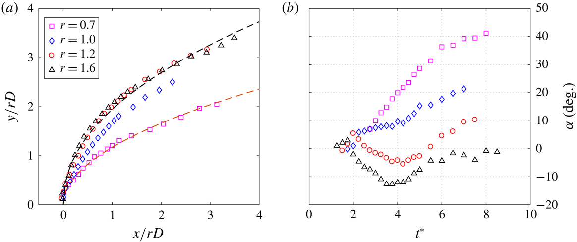
For steady jets, jet trajectories are commonly defined as the time-averaged streamline that originates from the exit centre, or positions of local velocity maxima, scalar maxima or vorticity maxima (Mahesh Reference Mahesh2013). However, for PSJs, the definition of jet trajectories is not straightforward. In Zong & Kotsonis (Reference Zong and Kotsonis2017c ), the envelope of the middle streamlines at different ejection phases were extracted to fit the jet trajectory with
 $$\begin{eqnarray}\frac{y}{rD}\,=\,A\left(\frac{x}{rD}\right)^{B}.\end{eqnarray}$$
As shown in figure 12(a), this streamline definition yields a jet trajectory (
 $A=2.2$
,
 $B=0.25$
) that is lower than the trace of the vortex ring centre in the far field (
 $A=2.0$
,
 $B=0.45$
). For steady jets, typical ranges for the two coefficients in (4.4) are
 $1.2<A<2.6$
and
 $0.28<B<0.34$
(Margason Reference Margason1993). Thus, it is evident that the high penetration ability of pulsed jets in cross-flow is actually contributed by the vortex rings. This observation has been utilized by M’Closkey et al. (Reference M’Closkey, King, Cortelezzi and Karagozian2002) to maximize the jet penetration by optimizing the time-varying exit velocity. The time variation of the back-flow area (
 $A_{b}$
) in the leeward side of the jet body as well as the mean velocity in this region (
 $U_{b}$
) is shown in figure 12(b). As a result,
 $A_{b}/D^{2}$
increases linearly during the primary jet stage (
 $t^{\ast }\leqslant 4$
) and decreases after the jet diminishes. The peak value of
 $A_{b}/D^{2}$
is approximately 2. This variation trend is attributed to the wax and wane of the virtual blockage effect created by the erect high-speed jet body. By contrast, the mean back-flow velocity experiences a monotonically decreasing trend, and a plateau of
 $0.5U_{\infty }$
is observed at
 $2\leqslant t^{\ast }\leqslant 4$
.
Spatial–temporal map of the boundary-layer shape factor in the
 $xy$
-plane. The black thin lines and blue dashed lines are contour lines of
 $H=1.4$
(baseline value) and
 $H=1.37$
, respectively. The white arrow indicates a propagation velocity of
 $0.7U_{\infty }$
.

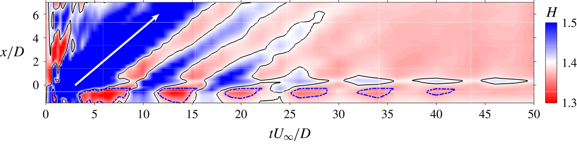
Phase-averaged effects of PSJ on the turbulent boundary layer in the symmetry plane can be illustrated from the spatial–temporal map of the boundary-layer shape factor, as shown in figure 13. Note that the shape factor under the baseline condition is 1.40. Blue and red colours indicate degradation (i.e. deceleration) and energization (i.e. acceleration) of the boundary layer, respectively. The upright high-speed jet and the leeward back-flow region incur significant momentum deficits to the near-exit boundary layer at
 $t^{\ast }<7$
. This momentum-deficit area travels downstream at approximately
 $0.7U_{\infty }$
and creates a parallelogram of high boundary-layer shape factor. Similar narrow streaks are formed when the secondary weak jets are issued. Upstream of the jet exit, several spots of low shape factor occur periodically along the time axis, which is associated with the fluctuating suction velocity as shown in figure 7(b). The period of these spots corresponds to the Helmholtz natural oscillation period (approximately
 $600~\unicode[STIX]{x03BC}\text{s}$
). Additionally, as weak suction dominates the later evolution of PSJs (see figure 7), the right half of the map is dominated by boundary-layer energization.
(a) Contours lines of the time-averaged streamwise velocity: –
 $\cdot$
–, baseline condition; ——, case 4. From the top down,
 $U_{x}/U_{\infty }$
varies from 0.9 to 0.5 in steps of
 $-0.1$
. The blue dashed curve shows the jet trajectory fitted from the trace of the vortex ring centre. (b) Streamwise variation of normalized wall shear stress and boundary-layer shape factor in time-averaged flow field: – – –,
 $k_{\unicode[STIX]{x1D70F}}$
; ——,
 $H$
. Boundaries of the jet exit are indicated by two thin lines. The baseline value for
 $H$
is 1.4.

Figure 14(a) shows the time-averaged velocity field reconstructed with (3.2). Upstream of the jet orifice, velocity contours are shifted to the near-wall region by suction flow, while a time-averaged reduction of the boundary-layer shape factor is perceived, as shown in figure 14(b). For velocity contour lines of
 $0.5\leqslant U_{x}/U_{\infty }\leqslant 0.7$
, a distortion is manifested right underneath the jet trajectory fitted from the vortex ring centre trace. This region corresponds to the time-averaged momentum deficit caused by the back-flow area and the lifting jets, leading to high shape factor (
 $H>1.4$
, retarded flow) between
 $0.5<x/D<2$
. After
 $x/D>2$
, the shape factor remains unchanged at the baseline value. Additionally, the variation of wall shear stress can be estimated from the velocity vector closest to the wall at approximately
 $y^{+}=10$
, as shown in the equation
 $$\begin{eqnarray}k_{\unicode[STIX]{x1D70F}}=\frac{U_{x}|_{y^{+}=10}}{U_{x0}|_{y^{+}=10}}.\end{eqnarray}$$
Here
 $U_{x}$
and
 $U_{x0}$
denote the streamwise velocity in case 4 and under baseline condition, respectively;
 $k_{\unicode[STIX]{x1D70F}}$
can be interpreted as the normalized wall shear stress, provided that the near-wall velocity gradient does not change considerably until
 $y^{+}=10$
. Particular attention should be drawn to the relative uncertainty in wall shear estimation, which can reach 15 % due to an ambiguous wall position (1 pixel). As a result, the wall shear stress is inversely proportional to the shape factor as expected, and an increase of up to 60 % is attained just upstream of the exit orifice. Downstream of the exit,
 $k_{\unicode[STIX]{x1D70F}}$
recovers from 0.8 to approximately 1.35 and remains unchanged afterwards. This elevated wall shear stress in the symmetry plane is also observed in the interaction between conventional synthetic jets and a laminar boundary layer (Jabbal & Zhong Reference Jabbal and Zhong2010).
4.2 Spanwise planes
Time evolution of the phase-averaged velocity fields at
 $x=2D$
(b,e,h). The corresponding velocity field in the symmetry plane is shown in (a,d,g). Dimensionless convection time: (a–c)
 $t^{\ast }=3$
; (d–f)
 $t^{\ast }=4$
; (g–i)
 $t^{\ast }=5.5$
. The thick red lines superimposed on contours indicate vortices detected with 10 % of the maximum
 $Q$
-value. The thin blue lines in (a,d,g) and the thin dark lines in (b,e,h) are contour lines of
 $U_{x}/U_{\infty }=-0.1$
and
 $U_{xyz}/U_{\infty }=1$
, respectively. The black dashed lines and red solid lines in (c,f,i) plot, respectively, the wall-normal variations of the upwash velocity at
 $x=2D$
,
 $z=0$
and the
 $Q$
-value variation along the white lines placed at the vortex centre in (a,d,g).

Phase-averaged velocity fields at
 $t^{\ast }=7$
: (a) symmetry plane; (b)
 $x=2D$
; (c)
 $x=5D$
. Thick red lines indicate vortices detected with a criterion of 10 % of the maximum
 $Q$
-value. Thin blue lines are contour lines of
 $U_{y}/U_{\infty }=0.2$
. In panel (a), arrows indicate the directions of in-plane periodic fluctuation velocity components, namely (
 $\tilde{u} _{x},\tilde{u} _{y}$
). As a comparison, arrows in panels (b) and (c) indicate the directions of in-plane phase-averaged velocity components (
 $U_{x},U_{y}$
).

Phase-averaged velocity fields at
 $x=2D$
for increasing time delays (
 $t^{\ast }=3$
, 4 and 5.5) are shown in figure 15(b,e,h). The corresponding velocity fields in the symmetry plane are displayed in figure 15(a,d,g) for comparison. In figure 15(c,f,i), wall-normal variations of
 $U_{y}/U_{y,max}$
at
 $x=2D$
,
 $z=0$
and normalized
 $Q$
-value variation along a wall-normal line that passes through the nearest vortex centres (white lines in figure 15
a,d,g) are plotted together;
 $U_{y,max}$
and
 $Q_{max}$
denote the peak values of
 $U_{y}$
and
 $Q$
-value, respectively. At
 $t^{\ast }=3$
, the FVR is located upstream of
 $x=2D$
, and the downwash effect of the downstream side of the FVR can be visualized clearly in figure 15(b). The position of peak downwash velocity corresponds well to the centre of the downstream vortex (
 $Q$
-value peak) as expected. The head of the high-speed jet is intersected by the spanwise measurement plane in a circular shape as indicated by the contour line of
 $U_{xyz}/U_{\infty }=1$
. Significant momentum deficit is observed underneath the jet head. At
 $t^{\ast }=4$
, the measurement plane of
 $x=2D$
cuts through the vortex ring. As a result, a CVP is perceived in figure 15(e), corresponding to the two longitudinal edges of the ring. The position of the peak upwash velocity is slightly higher than that of the downstream vortex centre, which can be ascribed to the downstream tilting of the FVR as described in § 4.1. The high-momentum flow entrained in the ring is spread outwards and upwards, leading to a mushroom-shaped cross-section of the high-speed jet.
At
 $t^{\ast }=5.5$
, the measurement plane of
 $x=2D$
intersects with the upstream portion of the ring, and three CVPs are detected in figure 15(h). The top one is the cross-section of the ring, featuring a double-lobed jet body underneath. The middle one appears to be connected with the reverse flow area, and is inferred as a cross-section of the inclined HVP (Zong & Kotsonis Reference Zong and Kotsonis2017c
). Specifically, this HVP is generated by the shear between the main flow and the reverse flow. It resides in the leeward side of the jet body and initially orients in the wall-normal direction (
 $t^{\ast }=3$
) (Yuan & Street Reference Yuan and Street1998; Meyer et al.
Reference Meyer, Pedersen and Özcan2007). While the jet body bends to the cross-flow, the HVP tilts accordingly (figure 8
g) and evolves into a quasi-streamwise CVP underneath the FVR. This vortex pair rotates in the same direction as the two longitudinal edges of the ring, and induces a downwash velocity at its two sides (
 $z/D>1$
and
 $z/D<-1$
). This downwash effect sweeps the high-momentum flow in the outer boundary layer to the near-wall region and curves locally the streamwise velocity contour lines. Additionally, as this primary counter-rotating vortex pair (
 $p$
-CVP) resides in close proximity to the wall (approximately
 $y=2.4D$
), a secondary counter-rotating vortex pair (
 $s$
-CVP) located at
 $y=0.16D$
is induced. This
 $s$
-CVP rotates contrary to the primary CVP and induces a weak downwash velocity in the middle. This flow scenario is consistent with that of conventional synthetic jets in a laminar boundary layer at large velocity and stroke ratio (Zhou & Zhong Reference Zhou and Zhong2009; Jabbal & Zhong Reference Jabbal and Zhong2010).
Time evolution of the circulation of a
 $p$
-CVP and the circulation difference between upstream and downstream sides of the FVR.

Phase-averaged velocity fields at
 $t^{\ast }=7$
in both symmetry and spanwise planes (
 $x=2D$
,
 $5D$
) are shown in figure 16. Note that the vector arrows in figure 16(a) correspond to the direction of in-plane periodic fluctuation velocity components, (
 $\tilde{u} _{x},\tilde{u} _{y}$
). Namely, the time-averaged motion has been subtracted, and only the relative change brought by PSJs at this specific phase remains. As a result, two regions with significant lifting motion (
 $U_{y}/U_{\infty }>0.2$
) are perceived. One is located in the middle of the FVR, and the other is induced by the
 $p$
-CVP. These two vortical structures are detected respectively in the measurement plane of
 $x=2D$
and
 $x=4D$
. Based on the mean vector direction in the bottom upwash region in figure 16(a), the inclination angle of the
 $p$
-CVP at this phase is estimated to be
 $45^{\circ }$
. Additionally, the two upwash regions in the symmetry plane seem to be jointed together, indicating the possible connection between the two vortical structures (FVR and
 $p$
-CVP).
Pseudo-3D vortical structures generated by PSJs in cross-flow at
 $r=1.6$
: (a) axonometric view; (b) top view; (c) side view.

Simulation results in Zhou & Zhong (Reference Zhou and Zhong2009) demonstrated that, for conventional synthetic jets in a laminar incoming boundary layer (
 $r=1.04$
,
 $L^{\ast }=2.7$
; under equivalent definition), this primary CVP is branched from the middle of the FVR, and extends downwards to the wall. As circulation is conserved within a vortex tube (Wu, Ma & Zhou Reference Wu, Ma and Zhou2007), the branch of the
 $p$
-CVP from the FVR will lead to a different circulation between the upstream and downstream sides of the ring. This difference in circulation (
 $\unicode[STIX]{x0394}\unicode[STIX]{x1D6E4}=\unicode[STIX]{x1D6E4}^{-}-\unicode[STIX]{x1D6E4}^{+}$
; see figure 11
b) should be compensated by the circulation of the
 $p$
-CVP (denoted by
 $\unicode[STIX]{x1D6E4}_{p}$
). To validate this conjecture, the time evolutions of
 $\unicode[STIX]{x1D6E4}_{p}$
and
 $\unicode[STIX]{x0394}\unicode[STIX]{x1D6E4}$
are plotted together in figure 17. As a result, the dimensionless circulation of
 $p$
-CVP pivots around 0.25 between
 $t^{\ast }=5.5$
and
 $t^{\ast }=7.5$
, which is in close proximity to the mean value of
 $\unicode[STIX]{x0394}\unicode[STIX]{x1D6E4}/rDU_{\infty }$
(0.19). This confirms the interconnection between the FVR and the
 $p$
-CVP. The residual between these two circulation values can be attributed to the different thresholds of vortex detection as well as the inclined orientation of the
 $p$
-CVP.
Assembling the stereo-PIV results measured at the same location (
 $x=2D$
) but increasing time delays, a three-dimensional (3D) dataset spreading along
 $t$
,
 $y$
and
 $z$
directions can be constructed. Contour surfaces of streamwise vorticity and downwash velocity in this space are plotted in figure 18 to visualize the pseudo-3D vortical structures (FVR,
 $p$
-CVP and
 $s$
-CVP). Different views are provided, and the organizations of these vortical structures agree with the earlier analysis. Based on Taylor’s frozen turbulence hypothesis (Taylor Reference Taylor1938), these pseudo-3D structures can represent the physical flow topology only if negligible deformation is exhibited during downstream convection. Namely, the material derivatives are approximately zero,
 $\text{d}U_{i}/\text{d}x\approx 0$
. In this study, this prerequisite is violated by the noticeable lifting motion of the FVR and the bending of the
 $p$
-CVP between
 $2<t^{\ast }<15$
, which should be corrected while projecting these pseudo-vortical structures back to physical 3D space (
 $x,y,z$
). Specifically, the downstream tilting of the FVR is exaggerated in the side view, and should be less than
 $13^{\circ }$
based on figure 11. The spatial orientation of
 $p$
-CVP is also far from level and should be highly inclined (
 $45^{\circ }$
at
 $t^{\ast }=7$
). Notwithstanding these considerations, pseudo-3D visualizations serve as valuable topological interpretations of the pertinent flow behaviour.
It is striking to note that, in figure 18(b), the two downwash streaks induced by the
 $p$
-CVP are connected at the tail at approximately
 $tU_{\infty }/D=10$
. This connection indicates that the two ends of the
 $p$
-CVP are jointed by spanwise vortices, namely SVs. SVs are generated in the windward side of the jet body (Kelso et al.
Reference Kelso, Lim and Perry1996) and have already been identified by the
 $Q$
-criterion in figure 15(a,d), as well as in figure 16(a). These SVs are inferred to be in an arch shape and seated on the
 $p$
-CVP (HVP), as will be detailed later on in § 6.
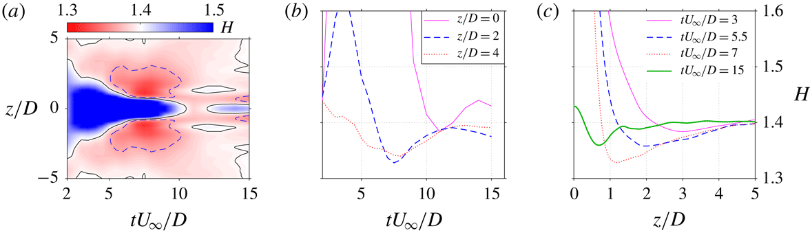
The spatial–temporal map of the boundary-layer shape factor measured at
 $x/D=2$
is shown in figure 19(a). Contour lines of
 $H=1.4$
and
 $H=1.37$
are extracted to assist the interpretation. A triangular region with high shape factor (
 $H>1.4$
) is observed at
 $t^{\ast }<10$
, which corresponds to the significant momentum deficit incurred by the diminishing reverse flow. In the two sides of this triangular region (
 $5<t^{\ast }<10$
), low shape factor (
 $H<1.4$
) is manifested, as a result of the downwash effect of the
 $p$
-CVP. This downwash effect is most significant in the spanwise extent of
 $1<|z/D|<3$
and diminishes completely at
 $|z/D|>5$
, which agrees with the large-eddy simulation (LES) results in Lardeau & Leschziner (Reference Lardeau and Leschziner2011). In figure 19(b,c), variations of the boundary-layer shape factor at several representative locations/time instants are plotted as curves. During the interval of
 $t^{\ast }\geqslant 12$
, the boundary-layer shape factor at
 $z/D=0$
rises with increasing time delay, whereas that at
 $z/D=2$
drops slightly. These variations can be associated with the weak secondary jet (see figure 8
i). Specifically, this secondary jet also induces a weak streamwise CVP in the near-wall region (not shown). Between and beside the two legs of this CVP, weak upwash and downwash effects are experienced respectively by the boundary layer, resulting in the aforementioned variations of shape factor.
(a) Spatial–temporal map of the boundary-layer shape factor at
 $x/D=2$
. The black thin lines and blue dashed lines are contour lines of
 $H=1.4$
(baseline value) and
 $H=1.37$
, respectively. (b) Time evolution and (c) spanwise variation of the boundary-layer shape factor at selected locations/time instants.

5 Effect of velocity ratio
In this section, the effect of velocity ratio on vortex ring evolution, jet penetration and boundary-layer shape factor is analysed in detail. Case 1 (
 $r=0.7$
) is taken as an example to illustrate the distinct flow topology that occurs at low velocity ratio.
5.1 Vortex ring evolution
The time evolution of the spanwise vorticity contours in case 1 (
 $r=0.7$
) is shown in figure 20. At
 $t^{\ast }\leqslant 2$
, incipient jets protrude from the exit orifice, displacing the boundary-layer vorticity upwards. In the vicinity of the exit orifice edges, positive and negative vorticity rolls into a vortex ring. This vortex ring breaks the constraints of the boundary-layer vorticity at
 $t^{\ast }=3$
and tilts upstream afterwards. This contrasts with the initial downstream tilting motion exhibited by case 4 and can be ascribed to the different stroke ratio. Specifically, the stroke ratio in case 1 (2.0) is smaller than the formation number (3.6) (Sau & Mahesh Reference Sau and Mahesh2007), and no trailing vorticity column is formed behind vortex rings as shown in figure 20(d). Consequently, vortex rings are isolated in the cross-flow, and upstream tilting driven by Kutta–Joukowski lift is exhibited.
Time evolution of vorticity contour at
 $r=0.7$
: (a)
 $t^{\ast }=1.5$
; (b)
 $t^{\ast }=2.0$
; (c)
 $t^{\ast }=3$
; (d)
 $t^{\ast }=4$
. Plotting methods are inherited from figure 10.

(a) Propagation of the FVR in cross-flow at
 $r=0.7$
: ○, windward vortex centre (
 $x_{v}^{+},y_{v}^{+}$
); ▵, leeward vortex centre (
 $x_{v}^{-},y_{v}^{-}$
). (b) Variation of the dimensionless vortex circulation (
 $\unicode[STIX]{x1D6E4}$
) in both quiescent air and cross-flow.

The spatial evolution of the FVR in cross-flow is shown in figure 21(a). The dimensionless circulations of the two sides of the ring in both quiescent and cross-flow conditions are plotted in figure 21(b). In contrast to the high-velocity-ratio case (case 4), the vortex ring stays in the vicinity of the jet exit (
 $x/D<3$
) and undergoes a significant upstream tilting with a peak pitching angle (
 $\unicode[STIX]{x1D6FC}$
) of approximately
 $40^{\circ }$
. The circulation of the upstream vortex (
 $\unicode[STIX]{x1D6E4}^{+}$
) is always lower than that of the downstream vortex (
 $\unicode[STIX]{x1D6E4}^{-}$
), and their difference can be interpreted from the boundary-layer vorticity. As shown in figure 20(c), part of the boundary-layer vorticity is entrained in the downstream side of the developing ring, leading to an increased positive circulation; whereas for the upstream side of the ring, part of the vorticity is cancelled out due to the reverse sign, resulting in a reduced negative circulation. The mean values of
 $\unicode[STIX]{x1D6E4}^{+}$
and
 $\unicode[STIX]{x1D6E4}^{-}$
roughly follow the trend of
 $\unicode[STIX]{x1D6E4}_{0}$
, indicating a comparable dissipation/mixing rate between quiescent and cross-flow conditions. This contrasts with case 4, where the dissipation rate of vortex ring circulation is evidently higher in cross-flow than that in quiescent condition. The distinct dissipation rate is associated with the different volume entrainment rate of vortex rings. In Sau & Mahesh (Reference Sau and Mahesh2008), the difference in volume entrainment rate between cross-flow and quiescent conditions is demonstrated to increase with stroke ratio. For low stroke length (
 $L^{\ast }<2$
, case 1), marginal difference (
 ${<}20\,\%$
) is expected, whereas for high stroke length (
 $L^{\ast }>4$
, case 4), this difference can reach up to 70 %. As a result, case 1 exhibits a comparable dissipation rate of circulation in cross-flow and quiescent conditions.
It must be noted that, during later evolution, the upstream vortex never ceases completely and can always be detected with decreasing threshold
 $Q$
-value. This observation contrasts with the results in Sau & Mahesh (Reference Sau and Mahesh2008) and Zhou & Zhong (Reference Zhou and Zhong2009), where HV are reported. Further comparisons will be provided in § 6.
(a) Normalized traces of the FVR at different velocity ratios. (b) Time variation of the pitching angle (
 $\unicode[STIX]{x1D6FC}$
) of the FVR.

A collective representation of vortex ring trajectories for all tested cases is shown in figure 22(a). As a result, the penetration ability of the vortex rings improves with velocity ratio at
 $r\leqslant 1.2$
and remains unchanged afterwards. Using (4.4) to fit the vortex ring trace at
 $r=0.7$
, the two coefficients are estimated to be
 $A=1.2$
and
 $B=0.50$
, which yields a trajectory lower than steady jets in the near field (
 $rD<10$
, reference value
 $A=1.9$
,
 $B=0.31$
) (Margason Reference Margason1993). This weak penetration ability in low velocity ratio can be traced back to the orientation of the emitted vortex rings. As shown in figure 22(b), the pitching angle of vortex rings (
 $\unicode[STIX]{x1D6FC}$
, positive value for upstream tilting) exhibits a similar variation trend at
 $r=1.2$
and
 $r=1.6$
, namely decreasing at
 $t^{\ast }<4$
and increasing afterwards. This variation trend is ascribed to the presence of the trailing vorticity column behind the vortex rings at large stroke ratio (
 $L^{\ast }>3.6$
) (§ 4.1). As the pitching angle pivots around
 $0^{\circ }$
in these two cases, the induced velocity of the vortex rings always has a large component in the wall-normal direction, which favours fast penetration. As a comparison, the pitching angle at
 $r=0.7$
and
 $r=1.0$
increases monotonically to
 $20^{\circ }$
and
 $40^{\circ }$
, respectively. With increasing pitching angle, the wall-normal component of the induced velocity of the vortex rings decreases, which leads to weak penetration ability. For pulsed jets in laminar cross-flow with fixed velocity ratio (
 $r>2$
), the optimal stroke ratio for maximum jet penetration collapses onto a line that lies to the left side (smaller side) of the ‘transition stroke ratio’ (Sau & Mahesh Reference Sau and Mahesh2010).
5.2 Pseudo-3D vortex structure, boundary-layer shape factor and wall shear stress
In case 1 (
 $r=0.7$
), the pseudo-3D vortical structures constructed from the stereo-PIV results measured at
 $x=2D$
are shown in figure 23. Different from case 4, only a FVR and a near-wall secondary CVP are perceived. The primary CVP evolved from the HVP disappears. This is somehow expected and can be interpreted as follows. At large velocity ratio, reverse flow is formed in the leeward side of the jet due to the virtual blockage created by the erect high-speed jet body (see figure 10). The skewed mixing layer between the reverse and main flow evolves into a HVP residing in the leeward side of the jet (Yuan, Street & Ferziger Reference Yuan, Street and Ferziger1999; Meyer et al.
Reference Meyer, Pedersen and Özcan2007). At low velocity ratio, only the FVR is issued (figure 10), and the small reverse flow located underneath the downstream side of the ring diminishes rapidly after formation (
 $t^{\ast }>4$
). As such, no HVP is generated in the case of low velocity ratio. The
 $s$
-CVP residing in the near-wall region at
 $r=0.7$
is directly induced by the two longitudinal edges of the ring. In cases of
 $r=1.0$
and
 $r=1.2$
, the 3D vortex organization is similar to that at
 $r=1.6$
, and thus will not be detailed here.
Pseudo-3D vortical structures generated by PSJs in cross-flow at
 $r=0.7$
: (a) axonometric view; (b) top view; (c) side view.

For cases 1–3, spatial–temporal variations of the boundary-layer shape factor measured at
 $x=2D$
are shown in figure 24. The contours pertaining to different cases show morphological similarity. A region with high shape factor is observed in between
 $|x/D|<1$
and
 $2<t^{\ast }<10$
, corresponding to the momentum deficit created by the erect jet. Beside this region, there exist two cores of low shape factor, which can be ascribed to the downwash effect of either the FVR (case 4) or the
 $p$
-CVP (cases 1–3). These two cores are centred around
 $z=\pm 1D$
and
 $t^{\ast }=7.5$
, and expand with velocity ratio. In later phases (
 $t^{\ast }>12$
), a secondary jet manifests with another narrow band of low shape factor.
Spatial–temporal variations of the boundary-layer shape factor measured at
 $x=2D$
for increasing velocity ratio: (a)
 $r=0.7$
; (b)
 $r=1.0$
; (c)
 $r=1.2$
. Solid and dashed lines correspond to contour lines of
 $H=1.4$
and
 $H=1.37$
, respectively.

Streamwise variations of (a) time-averaged boundary-layer shape factor and (b) dimensionless wall shear stress in the symmetry plane for increasing velocity ratio. Two grey lines (
 $x=\pm 0.5D$
) are added to indicate the location of the exit orifice.

At different velocity ratios, streamwise variations of the time-averaged boundary-layer shape factor and normalized wall shear stress in the symmetry plane are shown in figure 25. Similar trends are shared by all the tested cases. Upstream of the exit orifice, lower shape factor is perceived, due to the removal of low-momentum flow at the inner boundary layer by suction. Downstream of the exit orifice, the shape factor rapidly increases, and a gradual recovery of
 $H$
to baseline value is exhibited after
 $x/D>3$
. The normalized wall shear stress follows an opposite trend to the boundary-layer shape factor, as expected. While velocity ratio decreases, the peak value of
 $k_{\unicode[STIX]{x1D70F}}$
drops. Nevertheless, a noticeable increase of approximately 10 % of
 $k_{\unicode[STIX]{x1D70F}}$
is still perceived downstream of the exit orifice at
 $r=0.7$
(case 1).
6 Conceptual model
A conceptual model of the two regimes of PSJs in cross-flow (representative cases 2–4 for regime A and case 1 for regime B) is shown in figure 26. For each regime, vortical structures in the near and far field with respect to the exit orifice are sketched. In regime A (
 $r>1$
,
 $L^{\ast }>2.6$
), a starting vortex ring is issued and followed by a trailing jet column. Owing to the asymmetric momentum addition, this starting vortex ring initially tilts downstream. SVs and an erect HVP are formed in the windward and leeward sides of this jet column, respectively. After the jet diminishes, the HVP bends with respect to the cross-flow and evolves into a quasi-streamwise
 $p$
-CVP that branches from the middle of the FVR and extends to the near-wall region. The two legs of the
 $p$
-CVP are bridged by weak SVs. Underneath the two legs of the
 $p$
-CVP, an
 $s$
-CVP is induced. Additionally, the downstream tilting of the FVR transforms to upstream tilting after the pinch-off of the trailing vorticity column. The timing of this transformation advances with decreasing velocity ratio. Particularly, the initial downstream tilting in case 2 is marginal. With regards to regime B, the FVR exhibits a consistent upstream tilting since formation. Both trailing jet column and
 $p$
-CVP are absent. The
 $s$
-CVP in the near-wall region is directly induced by the two longitudinal edges of the ring. The tail of the FVR is conjectured to be connected with boundary-layer vorticity, as the circulation in the upstream side of the ring is significantly lower than in the downstream side.
Conceptual models of PSJs in cross-flow. (a) Regime A, high velocity and stroke ratio. (b) Regime B, low velocity and stroke ratio.

Sau & Mahesh (Reference Sau and Mahesh2008) proposed a parameter map that classifies the possible flow regimes of pulsed jets in cross-flow. For comparison, the four cases tested in this study are indicated in this regime map, as shown in figure 27(a). A relatively good match is obtained, when the peak jet velocity is taken as reference velocity. The near-exit flow scenarios in cases 3 and 4, namely a downstream tilting vortex ring followed by a trailing jet column, are predicated reasonably in figure 27(a). In Sau & Mahesh (Reference Sau and Mahesh2008), the transition stroke ratio is defined as the non-dimensional stroke length where no significant upstream or downstream tilting of vortex rings is exhibited. Namely, the time-mean pitching angle of vortex rings is approximately zero. For the PSJs in the present study, this transition stroke ratio occurs between
 $L^{\ast }=3.7$
and
 $L^{\ast }=5.4$
(
 $3.7<L^{\ast }<5.4$
), which is higher than that of pulsed jets (red solid line in figure 27
a,
 $L^{\ast }=(3.6{-}5.6)\times \exp (-0.5r)$
) (Sau & Mahesh Reference Sau and Mahesh2008). Additionally, for pulsed jets in cross-flow at low velocity ratio (
 $r<2$
), a train of HV is expected, which deviates from the observation of upstream-tilting vortex ring in case 1. These differences can be attributed to the different Reynolds numbers. Specifically, both the boundary layer and PSJs are in the turbulent state in this experiment, with
 $Re_{\unicode[STIX]{x1D703}}=3000$
and
 $Re_{D}$
ranging from 1790 to 4300. For the simulation performed by Sau & Mahesh (Reference Sau and Mahesh2008),
 $Re_{D}$
is kept at 600, and a laminar boundary layer is prescribed as the inflow. The different thickness between turbulent and laminar boundary layers affects the degree to which the positive vorticity of the FVR is cancelled and finally the formation of vortical structures.
Possible flow regimes pertaining to (a) pulsed jets in cross-flow (Sau & Mahesh Reference Sau and Mahesh2008) and (b) conventional synthetic jets in cross-flow (Jabbal & Zhong Reference Jabbal and Zhong2008). Markers pertain to the present study: ▵, mean velocity ratio (
 $U_{p}/U_{\infty }$
) against stroke ratio; ○, peak velocity ratio (
 $U_{0}/U_{\infty }$
) against stroke ratio.

For conventional synthetic jets in cross-flow, three flow regimes including HV, SVR, and TDVR are demonstrated at different stroke length and velocity ratios (Jabbal & Zhong Reference Jabbal and Zhong2008), as shown in figure 27(b). Note that the reference velocity ratio in the original regime map has been doubled to match the definition in this study. As a result, cases 2–4 fall into the regime of TDVR, while case 1 is subject to the category of SVR. A conceptual model of TDVR is provided in Jabbal & Zhong (Reference Jabbal and Zhong2010) (figure 13 in their study), which is similar to the far-field flow scenario of PSJs in cross-flow sketched in figure 26(a), except for the absence of SVs. The flow scenario of SVR is featured by an upstream-tilting vortex ring highly elongated in the streamwise direction Jabbal & Zhong (Reference Jabbal and Zhong2008), which is also consistent with the conceptual model in figure 26(b), to some extent.
Jabbal & Zhong (Reference Jabbal and Zhong2010) visualized the wall shear stress of conventional synthetic jets in laminar cross-flow, using liquid crystals. In the regime of TDVR a single wide streak of high wall shear stress is observed in the symmetry plane, contrasting with the two narrow streaks perceived in other regimes. The formation of this single streak of high wall shear stress was ascribed to the downwash effect of
 $s$
-CVP by Jabbal & Zhong (Reference Jabbal and Zhong2010). However, based on our observations in figures 15(c), 19(a) and 24, the weak downwash effect of this
 $s$
-CVP prevailed between
 $4\leqslant t^{\ast }\leqslant 8$
is not able to counteract the negative effects brought by reverse flow, largely because the fluid swept to the near-wall region is degraded flow with low momentum. In the authors’ perspective, the presence of this streak of high wall shear stress in the symmetry plane is associated with the enhanced suction at high velocity ratio. Specifically, in the regimes of HV and SVR, the velocity ratio is relatively low and the amount of low-energy flow ingested by PSJAs is negligible. The two narrow streaks of high wall shear stress are a direct consequence of the downwash effect of the two legs of the FVR or HV. As velocity ratio increases, this suction effect prevails, and the wall shear stress upstream and downstream of the exit orifice is increased significantly (see figure 25), as a result of the removal of low-energy fluids in the inner boundary layer. Consequently, the gap between the two narrow streaks observed in regimes of the FVR or HV is filled, resulting in a wide streak of high wall shear stress, as observed in Jabbal & Zhong (Reference Jabbal and Zhong2008, Reference Jabbal and Zhong2010).
7 Conclusions
The present study examines the effect of velocity ratio (
 $r$
) on plasma synthetic jets (PSJs) issuing normally towards a turbulent boundary layer (
 $\unicode[STIX]{x1D6FF}_{99}/D=9.7$
,
 $Re_{\unicode[STIX]{x1D703}}=3000$
) in a range of
 $0.7<r<1.6$
. The Strouhal number based on the free-stream velocity and orifice diameter (
 $St=f_{d}D/U_{\infty }$
) is kept constant at 0.02. High-speed phase-locked PIV measurements are carried out in both the symmetry and spanwise planes (
 $z=0$
,
 $x=2D$
,
 $x=4D$
) to characterize the complete flow field evolution in one actuation cycle.
PSJs are created by periodically igniting a pulsed arc inside an enclosed cavity (pulse width
 $O(1~\unicode[STIX]{x03BC}\text{s})$
). Different from the sinusoidal exit velocity generated by conventional synthetic jets, the exit velocity of PSJs exhibits noticeable oscillations at the Helmholtz natural frequency (1.65 kHz in this study), leading to a multiple alternation between ejection and suction phases in one cycle. Two regimes are identified in the four tested cases, with distinct emitted vortex ring dynamics and flow topology.
Vortex ring dynamics directly determines the jet penetration. At high velocity and stroke ratio (
 $r=1.6$
,
 $L^{\ast }=5.4$
), vortex rings are followed by a high-speed trailing jet column and tilt downstream initially. The downstream tilting is attributed to an uneven momentum injection received by the upstream and downstream sides of the vortex rings. After the pinch-off of the jet column from the ring, the downstream tilting is transformed into an upstream tilting driven by Kutta–Joukowski lift. As a comparison, in the case of low velocity and stroke ratio (
 $r=0.7$
,
 $L^{\ast }=2.0$
), the vortex rings always tilt to upstream and the pitching angle increases monotonically. A maximum penetration is demonstrated when the mean pitching angle approximates zero (cases 3 and 4). The transition stroke ratio for PSJs (3.7–5.4) is higher than that for pulsed jets.
The near-wall flow topology affects the boundary-layer shape factor and wall shear stress. At high velocity and stroke ratio (
 $r\geqslant 2.1$
,
 $L^{\ast }\geqslant 2.6$
), several SVs and a reverse flow region are observed in the windward and leeward sides of the jet body, respectively. The reverse flow region accommodates a HVP which evolves into a quasi-streamwise
 $p$
-CVP after the jet terminates. On the sides of the two legs of this
 $p$
-CVP, a downwash velocity is induced, which creates a region with low shape factor. Low-momentum flow originating from the reverse flow is trapped in the middle of the
 $p$
-CVP and FVR, leading to a high boundary-layer shape factor in the symmetry plane. At low velocity ratio, no
 $p$
-CVP is formed. Nevertheless, a similar downwash effect is experienced beside the two longitudinal edges of the vortex rings. Consequently, similar spatial distributions of boundary-layer shape factor are exhibited. In the symmetry plane, the time-averaged wall shear stress is always higher than the baseline value and can be attributed to the removal of low-energy fluids during suction phases. As the velocity ratio increases, the time-averaged wall shear stress also increases.
In future steps, the regime map of PSJs in cross-flow should be completed with more data points in the top left and bottom right corners of the
 $L^{\ast }$
–
 $r$
space (see figure 27). The effect of Strouhal number, free-stream Reynolds number, relative boundary-layer thickness, as well as jet orientation (i.e. skew and inclination angle) should be identified. Additionally, comparisons between the experimental data obtained in this investigation and the results from LES or DNS are recommended to explore the physics of PSJs in cross-flow at a deeper level and over a broader range, particularly the effect of low jet density on the mixing rate and penetration ability of PSJs.