1 Introduction
Boundary layers spontaneously emerge in many space and astrophysical plasmas, typically in the presence of two interacting different plasma environments. That is the case of the solar wind interacting with self-generated or induced magnetospheres of various solar system objects, of the interaction between the local interstellar medium and the heliopause or of astrophysical jets interacting with the surrounding environment, just to mention a few. Such layers typically exhibit large-scale variations of magnetic, density and/or velocity fields. Because those gradients represent a source of free energy for a variety of plasma instabilities, their evolution feeds back into the global evolution of such systems. A typical situation of interest for the above-mentioned cases is provided by the boundary layer forming between two different magnetized plasma flows, as it occurs in planetary magnetopauses (e.g. Fujimoto et al. Reference Fujimoto, Mukai, Kawano, Nakamura, Nishida, Saito, Yamamoto and Kokubun1998; Hasegawa et al. Reference Hasegawa, Fujimoto, Maezawa, Saito and Mukai2003; Masters et al. Reference Masters, Achilleos, Cutler, Coates, Dougherty and Jones2012; Cerri et al. Reference Cerri, Henri, Califano, Del Sarto, Faganello and Pegoraro2013; Haaland et al. Reference Haaland, Reistad, Tenfjord, Gjerloev, Maes, DeKeyser, Maggiolo, Anekallu and Dorville2014; Liljeblad et al. Reference Liljeblad, Karlsson, Raines, Slavin, Kullen, Sundberg and Zurbuchen2015; Cerri Reference Cerri2018; Malara, Pezzi & Valentini Reference Malara, Pezzi and Valentini2018). In particular, such shear flows can be unstable to Kelvin–Helmholtz instability (KHI), developing the characteristic fully rolled-up vortex structures (e.g. Nakamura & Fujimoto Reference Nakamura and Fujimoto2005; Henri et al. Reference Henri, Cerri, Califano, Pegoraro, Rossi, Faganello, Šebek, Trávníček, Hellinger and Frederiksen2013; Faganello & Califano Reference Faganello and Califano2017). Signatures of possible KHI structures have been indeed observed at several planetary magnetopauses (see e.g. Hasegawa et al. Reference Hasegawa, Fujimoto, Phan, Rème, Balogh, Dunlop, Hashimoto and TanDokoro2004; Sundberg et al. Reference Sundberg, Boardsen, Slavin, Anderson, Korth, Zurbuchen, Raines and Solomon2012; Delamere et al. Reference Delamere, Wilson, Eriksson and Bagenal2013; Paral & Rankin Reference Paral and Rankin2013; Liljeblad et al. Reference Liljeblad, Sundberg, Karlsson and Kullen2014; Gershman et al. Reference Gershman, Raines, Slavin, Zurbuchen, Sundberg, Boardsen, Anderson, Korth and Solomon2015). These vortices may in turn feed secondary instabilities, developing on the shoulder of the primary KHI. A typical example is provided by vortex-induced magnetic reconnection in various forms (e.g. Nakamura & Fujimoto Reference Nakamura and Fujimoto2008; Faganello, Califano & Pegoraro Reference Faganello, Califano and Pegoraro2009; Nakamura et al. Reference Nakamura, Daughton, Karimabadi and Eriksson2013; Nakamura & Daughton Reference Nakamura and Daughton2014; Fadanelli et al. Reference Fadanelli, Faganello, Califano, Cerri, Pegoraro and Lavraud2018), or by the development of pressure anisotropies able to trigger kinetic instabilities (e.g. De Camillis et al. Reference De Camillis, Cerri, Califano and Pegoraro2016). Moreover, when the two plasma flows have different densities, the Rayleigh–Taylor instability (RTI) may be triggered by the large-scale vortex motion (Matsumoto & Hoshino Reference Matsumoto and Hoshino2004; Faganello, Califano & Pegoraro Reference Faganello, Califano and Pegoraro2008a ,Reference Faganello, Califano and Pegoraro b ). At fluid scales, the RTI can also emerge as a primary instability because of the gravitational acceleration since the magnetosheath is denser than the magnetosphere. However, since the gravitational acceleration is small and because the magnetic field tends to stabilize, the RTI is usually much less considered than the KHI, except than in some special cases (Guglielmi, Potapov & Klain Reference Guglielmi, Potapov and Klain2010).
At kinetic scales, a lower-hybrid drift instability (LHDI) may also emerge from the density gradient itself (Gary Reference Gary1993; Daughton Reference Daughton2003; Daughton, Lapenta & Ricci Reference Daughton, Lapenta and Ricci2004). The LHDI is often observed in both spacecraft data (Mozer & Pritchett Reference Mozer and Pritchett2011; Norgren et al. Reference Norgren, Vaivads, Khotyaintsev and André2012; Graham et al. Reference Graham, Khotyaintsev, Vaivads, André and Fazakerley2014, Reference Graham, Khotyaintsev, Vaivads, Norgren, André, Webster, Burch, Lindqvist, Ergun and Torbert2017; Yoo et al. Reference Yoo, Jara-Almonte, Yerger, Wang, Qian, Le, Ji, Yamada, Fox and Kim2018, Reference Yoo, Wang, Yerger, Jara-Almonte, Ji, Yamada, Chen, Fox, Goodman and Alt2019) and laboratory experiments (Carter et al. Reference Carter, Ji, Trintchouk, Yamada and Kulsrud2001, Reference Carter, Yamada, Ji, Kulsrud and Trintchouk2002; Yoo et al. Reference Yoo, Yamada, Ji, Jara-Almonte, Myers and Chen2014, Reference Yoo, Na, Jara-Almonte, Yamada, Ji, Roytershteyn, Argall, Fox and Chen2017) and has been especially studied in the context of magnetic reconnection (Lapenta & Brackbill Reference Lapenta and Brackbill2002; Pritchett, Mozer & Wilber Reference Pritchett, Mozer and Wilber2012; Roytershteyn et al. Reference Roytershteyn, Daughton, Karimabadi and Mozer2012, Reference Roytershteyn, Dorfman, Daughton, Ji, Yamada and Karimabadi2013; Price et al. Reference Price, Swisdak, Drake, Cassak, Dahlin and Ergun2016; Le et al. Reference Le, Daughton, Chen and Egedal2017, Reference Le, Daughton, Ohia, Chen, Liu, Wang, Nystrom and Bird2018). As a consequence, the KHI and the LHDI are expected to compete and interact in a quite complex way since their fastest growing modes (FGM) grow at different scale lengths and with different growth rates. The dynamics arising from such a competition and its nonlinear development is the main focus of this paper.
The KHI is a fluid-scale instability growing in a sheared flow. Its growth rate is controlled by the velocity shear and the corresponding gradient scale length (Chandrasekhar Reference Chandrasekhar1961; Miura & Pritchett Reference Miura and Pritchett1982; Faganello & Califano Reference Faganello and Califano2017). On the other hand, the LHDI is a kinetic-scale instability. This instability is driven by the coupling of ion thermal gyration with the free energy provided by the ion density gradient drift velocity. At scales where ions are demagnetized but electrons still frozen-in, this free energy efficiently feeds lower-hybrid waves through an inverse ion damping that makes these waves unstable (Gary Reference Gary1993). The growth rate is controlled by the frequency ratio between the electron plasma frequency and the cyclotron frequency, the plasma beta and the density gradient. In this work, we will mainly focus on the latter.
Due to the different typical scale lengths at which the KHI and the LHDI develop, the interplay between these instabilities has not yet been observed. The KHI including a density gradient has been investigated either by adopting a magnetohydrodynamic model (Takagi et al.
Reference Takagi, Hashimoto, Hasegawa, Fujimoto and TanDokoro2006; Faganello et al.
Reference Faganello, Califano and Pegoraro2008a
; Matsumoto & Seki Reference Matsumoto and Seki2010; Leroy & Keppens Reference Leroy and Keppens2017) or by adopting a hybrid kinetic model but neglecting electron inertia (Gingell, Sundberg & Burgess Reference Gingell, Sundberg and Burgess2015). In this case, however, the LHDI cannot grow since the FGM scales as
 $k_{\text{FGM}}\propto (m_{i}/m_{e})^{1/2}$
(Gary & Sgro Reference Gary and Sgro1990), where
 $k_{\text{FGM}}$
is the wave number associated to the FGM and
 $m_{i}/m_{e}$
the mass ratio between ions and electrons, and stabilizes more and more when the density gradient scale length becomes larger than a few ion inertial lengths (Gary Reference Gary1993). There also exist some fully kinetic simulations theoretically able to develop LHDI but none of them has actually shown evidence of it, either because the layer is too large (Matsumoto & Hoshino Reference Matsumoto and Hoshino2006; Umeda et al.
Reference Umeda, Miwa, Matsumoto, Nakamura, Togano, Fukazawa and Shinohara2010), or because the KHI have been excited to grow quicker (Matsumoto & Seki Reference Matsumoto and Seki2010; Umeda, Ueno & Nakamura Reference Umeda, Ueno and Nakamura2014). As a consequence, no simulation of KHI has ever reported the growth of LHDI in a space plasma. On the other hand, kinetic simulations of KHI revealed another kinetic effect: the dawn–dusk asymmetry, which impacts the growth of the KHI depending on the sign of
 $\boldsymbol{B}\boldsymbol{\cdot }\unicode[STIX]{x1D734}$
, where
 $\unicode[STIX]{x1D734}$
is the vorticity of the layer (Nakamura, Hasegawa & Shinohara Reference Nakamura, Hasegawa and Shinohara2010; Henri et al.
Reference Henri, Cerri, Califano, Pegoraro, Rossi, Faganello, Šebek, Trávníček, Hellinger and Frederiksen2013; Paral & Rankin Reference Paral and Rankin2013).
In this work, in order to investigate the interplay between the KHI and LHDI, we make use of a kinetic model of a boundary layer characterized by the presence of (i) a velocity shear that would be unstable to the KHI and (ii) a density gradient that would be unstable to the LHDI. We take the scale lengths of variation of the main fields (densities, magnetic field and velocities) of the order of the ion inertial length and vary their respective values. These configurations allow us to study the relative impact of each instability in the layer and on the plasma mixing.
The present paper is organized as follows. Section 2 describes the numerical model used in this paper. Section 3 presents the results, and is split into the different phases of the simulations. Section 3.1 shows the linear growth of the LHDI, when applicable, and the comparison of our numerical results with linear theory. Section 3.2 contains the nonlinear phase of the LHDI and describes the presence of an inverse cascade of energy responsible for the formation of large-scale structures. In some parameter regimes, those structures are shown to interfere with the growth of the KHI that develops on larger time scales. This feature, together with the factors playing a role in the competition between the nonlinear phase of the LHDI and the linear growth of the KHI, is studied in § 3.3. In § 4, we discuss the results of this paper and the inherent limitations of the used model. Finally, in § 5, we present a summary of this study, together with a description of possible consequences for the dynamics of planetary magnetospheres, such as the Hermean magnetopause.
2 Numerical set-up
We present four fully kinetic simulations in a two-dimensional (2-D) Cartesian geometry using the particle-in-cell (PIC) code SMILEI (Derouillat et al. Reference Derouillat, Beck, Pérez, Vinci, Chiaramello, Grassi, Flé, Bouchard, Plotnikov and Aunai2018). The simulations model the boundary between two plasmas characterized by different densities and separated by a velocity shear. Simulations are performed in the reference frame where the low-density plasma medium is at rest.
The data presented are normalized using ion-scale quantities. The magnetic field and density are normalized to arbitrary values
 $B_{0}$
and
 $n_{0}$
, respectively. We choose
 $B_{0}$
and
 $n_{0}$
such that the density and magnetic field are equal to 1 on the flowing side of the layer (in our simulations: the right side). The masses and charges are normalized to the proton mass
 $m_{p}$
and charge
 $e$
, time is normalized to the inverse of the proton gyrofrequency
 $\unicode[STIX]{x1D714}_{ci}^{-1}=m_{p}/eB_{0}$
and length to the proton inertial length
 $\unicode[STIX]{x1D6FF}_{i}=c/\unicode[STIX]{x1D714}_{pi}$
, where
 $c$
is the speed of light and
 $\unicode[STIX]{x1D714}_{pi}=\sqrt{n_{0}e^{2}/m_{p}\unicode[STIX]{x1D716}_{0}}$
is the proton plasma frequency. Velocities are normalized to the ions’ Alfvén velocity
 $v_{\text{Al}}=\unicode[STIX]{x1D6FF}_{i}\unicode[STIX]{x1D714}_{ci}$
.
Magnetic field ratio (
 $B_{r}$
), density ratio (
 $n_{r}$
) and velocity difference (
 $\unicode[STIX]{x0394}v_{\text{shear}}$
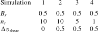
) values characterizing the discontinuity between the two adjacent plasmas, for the 4 simulations. Simulation 2 parameters correspond to parameters consistent with Mercury’s magnetopause (Slavin et al.
Reference Slavin, Acuña, Anderson, Baker, Benna, Gloeckler, Gold, Ho, Killen and Korth2008).

All simulations are initialized with a single layer where density, velocity (directed along the
 $y$
-direction) and magnetic field (directed along the
 $z$
-direction) vary along the
 $x$
direction. This layer is contained in the
 $(x,y)$
plane in a 2-D domain of size
 $(x_{\text{max}},y_{\text{max}})=(68,136)\unicode[STIX]{x1D6FF}_{i}$
. There are
 $n_{x}=n_{y}=2720$
cells in the
 $x$
and
 $y$
directions, corresponding to a grid resolution of
 $\unicode[STIX]{x1D6E5}_{x}=0.025\unicode[STIX]{x1D6FF}_{i}$
and
 $\unicode[STIX]{x1D6E5}_{y}=0.05\unicode[STIX]{x1D6FF}_{i}$
.
The ion and electron distribution functions are initially composed by
 $50$
macro-particles per cell loaded using Maxwellian distributions. Plasma moments and electromagnetic forces are calculated using second-order interpolation. The time step is calculated using a Courant–Friedrichs–Lewy condition, which in our simulations turns out to be
 $\unicode[STIX]{x1D6E5}_{t}=8.4\times 10^{-4}\unicode[STIX]{x1D714}_{ci}^{-1}$
, and the total simulation time is
 $400\unicode[STIX]{x1D714}_{ci}^{-1}$
. The boundary conditions are periodic in the
 $y$
direction and reflective in the
 $x$
direction for both particles and fields.
The initial density profile is given by:
 $$\begin{eqnarray}\displaystyle n_{i}(x,y)=\frac{1}{n_{r}}\left[1+\frac{n_{r}-1}{2}\left(1+\tanh \left(\frac{x-x_{0}}{L}\right)\right)\right]+n_{\text{curr}}, & & \displaystyle\end{eqnarray}$$
where
 $n_{r}=n_{a}/n_{b}$
is the density ratio across the current sheet,
 $L$
the initial characteristic width of the layer, fixed at
 $L=1$
in this work, and
 $n_{\text{curr}}=\boldsymbol{J}^{2}/(e^{2}n_{0}v_{\text{Al}}^{2})$
a small correction to allow ions to carry part of the current in order to avoid inconsistencies (negative electron density in the case of a very strong magnetic field gradient). The subscripts
 $a$
and
 $b$
stand for the asymptotic values on each side of the layer. The values of
 $n_{r}$
are listed in table 1. The ion velocity is initialized as,
 $$\begin{eqnarray}\displaystyle \boldsymbol{v}_{i}(x,y)=\left[\frac{\unicode[STIX]{x0394}v_{\text{shear}}}{2}\left(1+\tanh \left(\frac{x-x_{0}}{L}\right)\right)\right]\boldsymbol{e}_{y}+\boldsymbol{v}_{\text{curr}}, & & \displaystyle\end{eqnarray}$$
where
 $\unicode[STIX]{x0394}v_{\text{shear}}=|v_{a}-v_{b}|$
is the velocity difference across the shear layer and
 $\boldsymbol{v}_{\text{curr}}=\boldsymbol{J}/(en_{i})$
a small correction to allow ions to carry part of the current, in order to avoid inconsistencies, as consistent with the density correction. The values of
 $\unicode[STIX]{x0394}v_{\text{shear}}$
are listed in table 1. The initial magnetic field profile is given by,
 $$\begin{eqnarray}\displaystyle \boldsymbol{B}(x,y)=\frac{1}{B_{r}}\left[1+\frac{B_{r}-1}{2}\left(1+\tanh \left(\frac{x-x_{0}}{L}\right)\right)\right]\boldsymbol{e}_{z}, & & \displaystyle\end{eqnarray}$$
where
 $B_{r}=|B_{a}/B_{b}|$
is the magnetic asymptotic field ratio across the current sheet. The values of
 $B_{r}$
are listed in table 1. From the curl of
 $\boldsymbol{B}$
we calculate the current
 $\boldsymbol{J}$
since in our model the displacement current is neglected. Finally, the electric field is initially set to,
 $$\begin{eqnarray}\displaystyle \boldsymbol{E}=-\boldsymbol{v}_{i}\times \boldsymbol{B}+\frac{1}{en_{i}}\boldsymbol{J}\times \boldsymbol{B}, & & \displaystyle\end{eqnarray}$$
which correspond to an Ohm’s law where the initial electron pressure gradient term has been neglected. The
 $\unicode[STIX]{x1D735}(P_{e})/en_{e}$
term in the generalized Ohm’s law is by far the smallest contribution to the electric field. To ease the implementation of the initial conditions, we have neglected the electron pressure gradient term, and later checked and confirmed that this term can be neglected. However, note that this simplified equation does not perfectly match Ohm’s law within the boundary, as we consider a charge separation (
 $n_{i}\neq n_{e}$
) associated with the electric field gradient (Pritchett & Coroniti Reference Pritchett and Coroniti1984). Finally, electron density
 $n_{e}=n_{i}-\unicode[STIX]{x1D735}\boldsymbol{\cdot }\boldsymbol{E}$
and mean velocity
 $\boldsymbol{v}_{e}=(\boldsymbol{J}-n_{i}\boldsymbol{v}_{i})/n_{e}$
consistently follow from
 $\boldsymbol{J}$
and the Maxwell equations.
The total scalar pressure
 $P=P_{i}+P_{e}$
is determined in order to preserve pressure balance. The electron to ion temperature ratio is taken constant and equal to
 $\unicode[STIX]{x1D703}=T_{e}/T_{i}=0.2$
. The plasma
 $\unicode[STIX]{x1D6FD}=2P/B^{2}$
is set equal to 1 in plasma ‘a’ (left side). A reduced mass ratio
 $m_{i}/m_{e}=25$
is used for computational reasons. The consequences of using a reduced mass ratio are explained in detail in § 4. We fix
 $\unicode[STIX]{x1D714}_{pe}/\unicode[STIX]{x1D714}_{ce}=4$
. To optimize the layer stability, we make use of finite Larmor radius correction in the simulation set-up, as described in Cerri et al. (Reference Cerri, Pegoraro, Califano, Del Sarto and Jenko2014).
3 Numerical results
The simulations are characterized by three main phases. In the first one, a lower-hybrid drift instability develops very fast in all simulations except in simulation 4, where no density gradient is present. In the second phase, the LHDI saturates and enters the nonlinear stage, which is characterized in simulations 1 and 2 by the growth of large-scale finger-like structures. Finally, in the last phase, the Kelvin–Helmholtz instability may develop depending on whether or not the nonlinear LHDI structures grew fast enough (i.e. to a sufficiently large amplitude) to destroy the coherence of the shear flow. In order to better illustrate the different phases, movies of the out-of-plane magnetic field time evolution are available for simulations 2, 3 and 4 as supplementary material available at https://doi.org/10.1017/S0022377819000758. In the following, we discuss how the system evolves in each of these phases for each simulation.
3.1 The linear LHDI phase
At the initial times of all simulations (except for simulation 4), we observe growing fluctuations along the layer at
 $x\simeq 34$
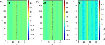
. In particular, in figure 1 we show the in-plane electron velocity component
 $v_{x}$
for simulations 1, 2 and 3, where the fluctuations length scale is observed at kinetic scale. Furthermore, the amplitude of fluctuations is bigger in simulations 1 and 2 than in simulation 3 since the instability depends on the density gradient (see table 1). Furthermore, a wave front propagating in the
 $x$
direction is clearly visible as a consequence of the absence of kinetic equilibrium at the layer’s initialization and our choice to neglect the pressure gradient term in (2.4). However, this artificial by-product of the initialization does not have a significant impact on the evolution of the simulation, as typically the case for kinetic simulation. Those waves are especially clear in simulation 3 since the colour scale amplitude has a reduced range with respect to simulations 1 and 2.
(a–c) In-plane electron velocity component
 $v_{x}$
at
 $t=7.5$
for simulations 1, 2 and 3, respectively. Simulation 4 is not plotted here because, in the absence of a density gradient, the LHDI does not develop, and consequently there are no visible fluctuations in the layer this early in the simulation.

To identify the instability as a LHDI, we compare our results with the corresponding linear theory. We solve the linear Vlasov equation under some simplified assumptions to compute the growth rate of the LHDI (Gary & Sanderson Reference Gary and Sanderson1978; Gary Reference Gary1983, Reference Gary1993). The simplifications are made in order to carry out the analytical model and are the following: density and temperature gradients much larger than ion gyro-radius, uniform out-of-plane magnetic field and a low plasma beta,
 $\unicode[STIX]{x1D6FD}=2P/B^{2}\ll 1$
. Our method consists in integrating the linearized Vlasov equation along unperturbed orbits, thus finding an expression for the dielectric function, and finally finding the zeros of this function numerically.
In our case, we have used a dielectric function
 $\unicode[STIX]{x1D700}(k,\unicode[STIX]{x1D714})$
of the form (Gary & Sanderson Reference Gary and Sanderson1979; Sgro, Peter Gary & Lemons Reference Sgro, Peter Gary and Lemons1989; Gary Reference Gary1993),
 $$\begin{eqnarray}\displaystyle \unicode[STIX]{x1D700}(k,\unicode[STIX]{x1D714}) & = & \displaystyle 1+\mathop{\sum }_{j}K_{j}(k,\unicode[STIX]{x1D714}),\end{eqnarray}$$
 $$\begin{eqnarray}\displaystyle \displaystyle K_{j}(k,\unicode[STIX]{x1D714}) & = & \displaystyle \frac{A_{j}^{2}}{k^{2}}\left(1-[\unicode[STIX]{x1D714}-kv_{nj}]\text{e}^{-k^{2}\unicode[STIX]{x1D70C}_{Lj}^{2}}\mathop{\sum }_{m=-\infty }^{+\infty }\frac{\text{I}_{m}(k^{2}\unicode[STIX]{x1D70C}_{Lj}^{2})}{\unicode[STIX]{x1D714}+m\unicode[STIX]{x1D714}_{cj}}\right.\nonumber\\ \displaystyle & & \displaystyle +\,\left.\frac{\unicode[STIX]{x1D714}v_{nj}}{kv_{\text{th},j}^{2}}\text{e}^{-k^{2}\unicode[STIX]{x1D70C}_{Lj}^{2}}\mathop{\sum }_{m=-\infty }^{+\infty }\frac{m\unicode[STIX]{x1D714}_{cj}\text{I}_{m}(k^{2}\unicode[STIX]{x1D70C}_{Lj}^{2})}{\unicode[STIX]{x1D714}+m\unicode[STIX]{x1D714}_{cj}}\right)\nonumber\\ \displaystyle & & \displaystyle -\,k^{3}\unicode[STIX]{x1D70C}_{Lj}^{2}v_{Tj}\text{e}^{-k^{2}\unicode[STIX]{x1D70C}_{Lj}^{2}}\mathop{\sum }_{m=-\infty }^{+\infty }\frac{\text{I}_{m}(k^{2}\unicode[STIX]{x1D70C}_{Lj}^{2})-\text{I}_{m}^{\prime }(k^{2}\unicode[STIX]{x1D70C}_{Lj}^{2})}{\unicode[STIX]{x1D714}+m\unicode[STIX]{x1D714}_{cj}},\end{eqnarray}$$
where
 $k$
and
 $\unicode[STIX]{x1D714}$
are the wave vector and frequency, respectively, and
 $K_{j}$
is the dielectric susceptibility of the species
 $j$
(the sum over
 $j$
running on all the species,
 $j=(i,e)$
in our case);
 $\text{I}_{m}$
are the modified Bessel functions of order
 $m$
. Moreover,
 $v_{\text{th},j}=\sqrt{T_{j}/m_{j}}$
and
 $\unicode[STIX]{x1D70C}_{Lj}=\sqrt{m_{j}T_{j}}/q_{j}B$
are the thermal velocity and the Larmor radius of the species
 $j$
, respectively, and
 $B$
is the magnetic field modulus. Finally
 $m_{j}$
and
 $q_{j}$
are the mass and charge of species
 $j$
, respectively, and
 $\unicode[STIX]{x1D714}_{cj}=q_{j}B/m_{j}$
is the gyrofrequency of the population
 $j$
. The drift velocities associated with the density (
 $n_{j}$
) and temperature (
 $T_{j}$
) gradients are defined as
 $v_{Fj}=\unicode[STIX]{x1D716}_{F}\unicode[STIX]{x1D70C}_{Lj}v_{\text{th},j}$
, where
 $F_{j}=(n_{j},T_{j})$
and
 $\unicode[STIX]{x1D716}_{F}=(1/F_{j}(x))\text{d}F_{j}(x)/\text{d}x$
. We also define
 $A_{j}=\unicode[STIX]{x1D714}_{pj}/v_{\text{th},j}$
. All the above formulas are in ion units (
 $\unicode[STIX]{x1D6FF}_{i}$
and
 $\unicode[STIX]{x1D714}_{ci}^{-1}$
).
As already said, this method assumes a gradient configuration with a density and temperature gradient length scale (
 $L_{F}\sim \unicode[STIX]{x1D716}_{F}^{-1}$
) much larger than ion gyro-radius (
 $\unicode[STIX]{x1D70C}_{Li}/L_{F}\ll 1$
), a uniform out-of-plane magnetic field and a low plasma beta,
 $\unicode[STIX]{x1D6FD}=2P/B^{2}\ll 1$
. Although those assumptions do not strictly hold in our simulations, the neglected effects would tend to slow down the process, so that we can consider the analytical theory as an upper limit for the growth rates and a useful reference for a comparison with simulation results in the linear regime (Davidson et al.
Reference Davidson, Gladd, Wu and Huba1977). Indeed, since
 $v_{nj}$
and
 $v_{Tj}$
are proportional to the density and temperature gradients, the LHDI growth rate is expected to be larger for steeper gradients of
 $n$
and
 $T$
. In the configuration adopted for the linear theory, we shall define the inverse gradient length
 $\unicode[STIX]{x1D716}_{T,n}$
as the one computed at
 $x\simeq x_{0}$
, i.e. at the initial location of the shear layer (see § 2).
The linear theory assumes a uniform magnetic field
 $B$
(and thus a uniform Larmor radius
 $\unicode[STIX]{x1D70C}_{Li}$
), while in the simulation the magnetic field is sheared. Therefore, we must fix a characteristic (mean) value of
 $\unicode[STIX]{x1D70C}_{Li}=\sqrt{\unicode[STIX]{x1D6FD}_{i}m_{i}/2en_{i}}\equiv \sqrt{\unicode[STIX]{x1D6FD}_{i}/2n_{i}}$
in normalized units. We take it as the local value at the centre of the magnetic gradient, i.e. at
 $x=x_{0}$
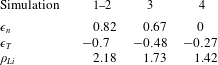
, and report the results in table 2.
Gradients and Larmor radius in the different simulations.

We have computed the dispersion relation using the parameters listed in table 2. The corresponding results, associated with the four kinetic simulations, are reported in figure 2.
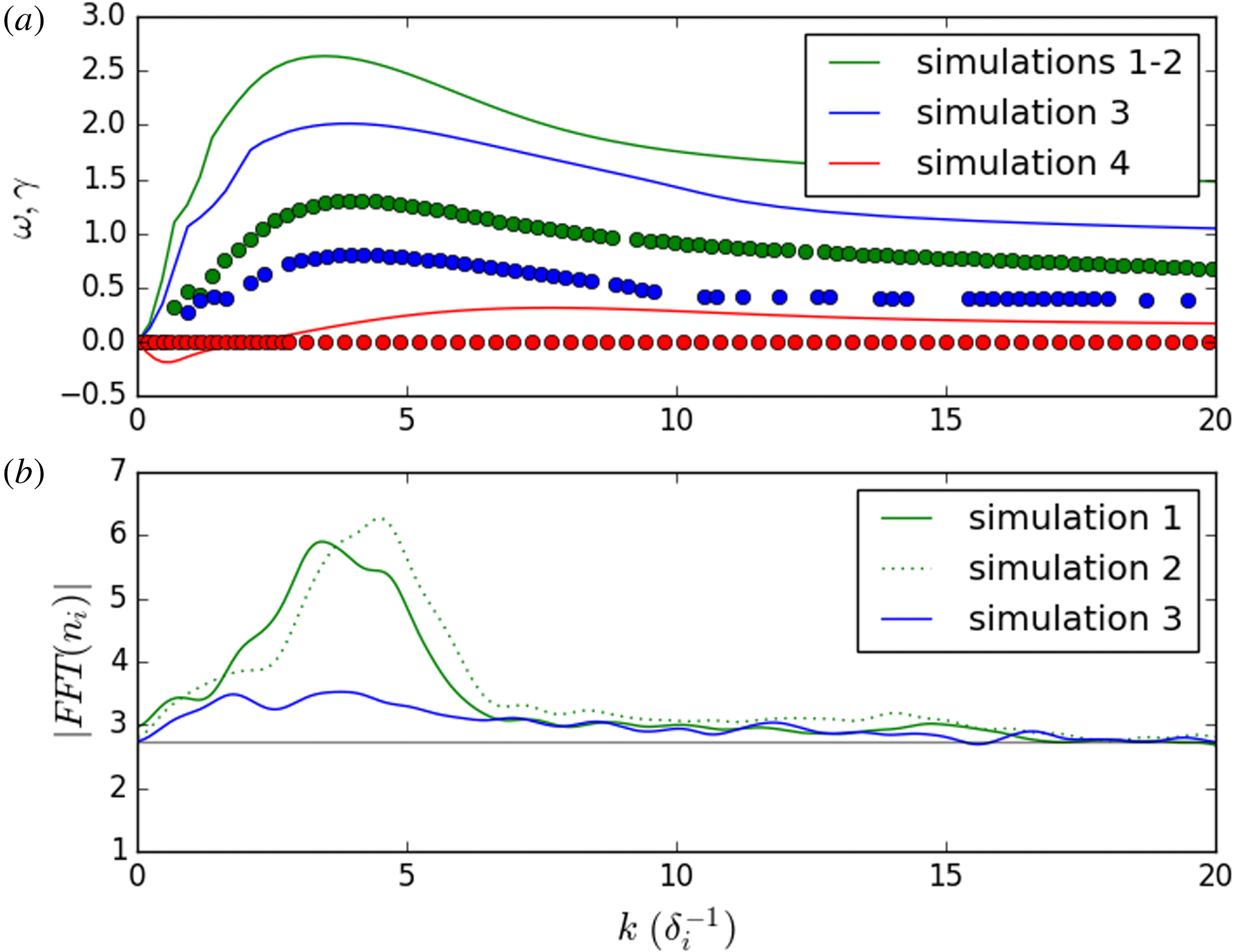
(a) Theoretical dispersion relation of the LHDI branch obtained from (3.2) with
 $m_{i}/m_{e}=25$
, and for the set of parameters given in table 2. The dotted lines represent the growth rate and the solid lines represent the real frequencies. (b) Fourier transform along
 $y$
of the density field at
 $x=34$
and
 $t=5$
for simulation 1, 2 and 3.

The main result emerging from figure 2(a) is that the LHDI is expected to grow on ion kinetic scales in simulations 1–3, while in simulation 4 the system is stable with respect to the LHDI. The LHDI fastest growing mode is
 $k_{\text{FGM}}=3.9$
for simulations 1–3, while the growth rate is
 $\unicode[STIX]{x1D6FE}_{\text{LHDI}}=1.3$
in simulation 1–2 and
 $\unicode[STIX]{x1D6FE}_{\text{LHDI}}=0.8$
in simulation 3 because of the different density gradients. In figure 2(b) we show the density spectrum observed in our simulations at
 $t=5$
. The peak around the FGM is in agreement with linear theory. On the other hand, simulation 4 does not develop any instability at such early times. As expected, the instability grows faster in simulation 1 and 2 than in simulation 3. We therefore conclude that the instability observed in the early stage of simulations 1, 2 and 3 corresponds to a LHDI.
The growth rate in the simulations is estimated by fitting the temporal evolution of the Fourier transform of
 $n_{i}$
(see figure 2
b) for
 $k=4$
(the fastest growing mode) during the linear phase of LHDI with an exponential function
 $A\text{e}^{t\unicode[STIX]{x1D6FE}_{\text{LHDI}}}$
. Quantitatively, the measured growth rates in simulations 1, 2 and 3 turn out to be smaller, by a factor of three, than the ones estimated by linear theory (see (3.2)). Such a discrepancy is explained by the inherent limitations of the theoretical model (Davidson et al.
Reference Davidson, Gladd, Wu and Huba1977), which considers a smooth density gradient, a uniform magnetic field and a low plasma
 $\unicode[STIX]{x1D6FD}$
. Finally, it is worth noticing that the presence of a velocity shear does not affect too much the instability, as shown in figure 2(b), where simulations 1, with no velocity shear, and 2, with a velocity shear, behave similarly.
3.2 The nonlinear LHDI phase
The LHDI ends its linear growth phase long before the KHI starts to develop, thus entering its nonlinear stage. In simulations 1 and 2, such a transition to the nonlinear regime occurs at
 $t_{NL}\sim 8$
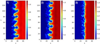
, eventually leading to an effective inverse cascade with the formation of many fluid-scale structures. This is shown in figure 3 where we draw the density contours for simulations 1, 2 and 3 in the nonlinear stage of the LHDI. Furthermore, in simulations 1 and 2 we observe the development of a new process associated with the inverse cascade that produces elongated finger-like structures entering from one plasma into the other. This is not observed in simulation 3 at similar times since the inverse cascade is less developed due to a slower growth of the LHDI. Such a phenomenon of finger-like structure generation is similar to what has been previously observed in kinetic simulations (Brackbill et al.
Reference Brackbill, Forslund, Quest and Winske1984; Gary & Sgro Reference Gary and Sgro1990; Singh & Leung Reference Singh and Leung1998).
Ion density at
 $t=150$
for simulations 1, 2 and 3.

As stated above, since in simulation 3 the LHDI is less efficient, the inverse cascade occurs later and is much less intense. Even though some finger-like features start to develop at later times, their growth is slower in simulation 3, on a time scale comparable to the growth of the KHI. Indeed, in this case, the competition between the growth of nonlinear LHDI structures and linear KHI actually prevents the finger-like structures from growing, eventually suppressing them completely once the KH vortices form. This last stage where KHI can develop will be further discussed in § 3.3.
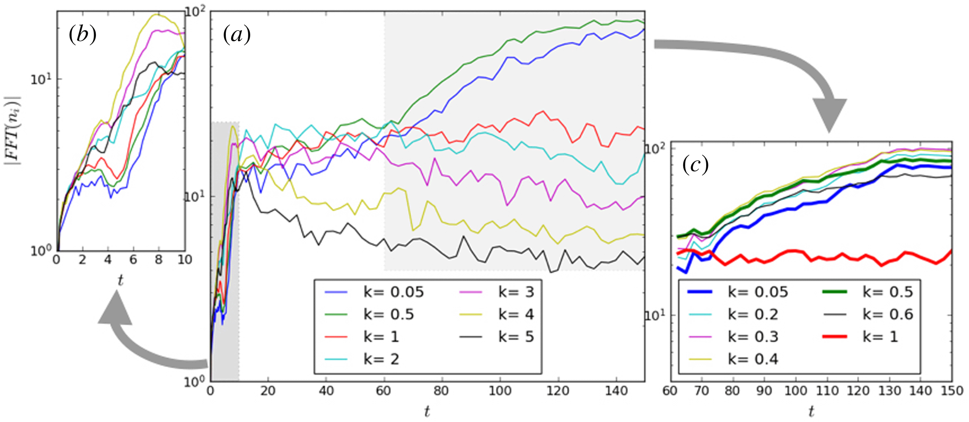
Time evolution of Fourier coefficient modulus of ion density fluctuations,
 $|\widehat{\unicode[STIX]{x1D6FF}n}_{i,k}(x)|=|\text{FFT}_{y}(n_{i})|$
, for some given
 $k$
at
 $x=33.25$
from simulation 1. Panels (a) and (b) share the same
 $k$
, while (c) plots another
 $k$
. The
 $k$
shared by all panels are plotted with thick lines in (c).

In figure 4(a) we show the time evolution of the modules of different Fourier coefficients for the density of simulation 1. Figure 4(b) shows a zoom of figure 4(a) at early times, when the energy growth is driven by the linear development of the LHDI. Figure 4(c) shows a zoom at late times of figure 4(a), although for other
 $k$
values. Figure 4(c) shows small
 $k$
(
 $k\leqslant 1$
) in order to show the evolution of the inverse cascade at large scales.
As discussed in § 3.1, the FGM of the LHDI is at approximately
 $k=4$
(yellow curve). However, in the nonlinear phase after
 $t_{NL}\sim 8$
, we observe that this mode stops growing and its associated energy starts to decrease. This transition marks the saturation phase of the LHDI and the beginning of the inverse-cascade phase which feeds the growth of lower
 $k$
modes. Indeed, after
 $t_{NL}$
, all wavenumbers larger than
 $k=4$
(yellow and black curves) decrease while smaller wavenumbers continue to grow. After some time, the low
 $k$
modes begin to decrease one after the other, except for
 $k<1$
, which continues to grow even faster. At longer times, we observe in figure 4(c) that the inverse cascade continues, with the energy evolving towards ever larger scales (i.e. smaller
 $k$
).
To calculate a characteristic time scale associated with the inverse cascade process and the corresponding growth of the fluid-scale structures, we measure the position
 $x_{0}(y)$
of the centre of the layer at any value of
 $y$
. To get
 $x_{0}(y)$
, we fit each cut along
 $x$
of the density with a hyperbolic tangent and take the inflection point of the fit as
 $x_{0}(y)$
. The time evolution of the standard deviation
 $\unicode[STIX]{x1D70E}_{0}=\sqrt{\langle x_{0}^{2}\rangle _{y}}$
gives an estimation of the growth of the finger-like structures.
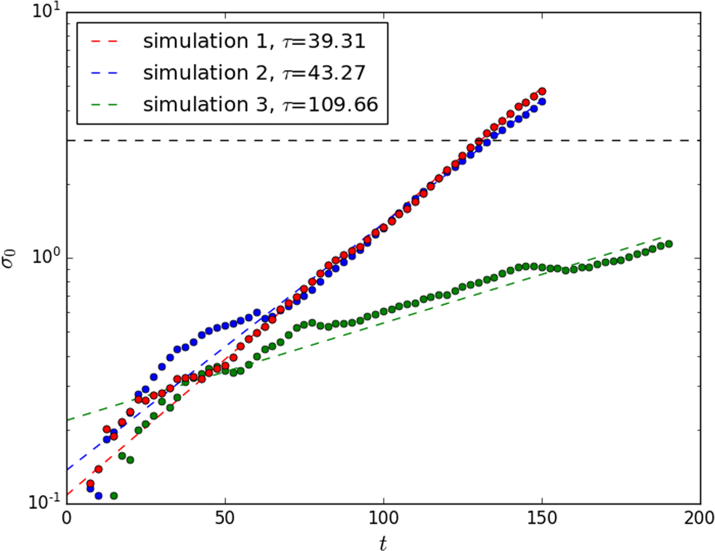
Time evolution of
 $\unicode[STIX]{x1D70E}_{0}=\sqrt{\langle x_{0}^{2}\rangle _{y}}$
from simulations (dots) and corresponding exponential fit (dashed lines). Different colours represent different simulations (see legend). The characteristic time
 $\unicode[STIX]{x1D70F}_{NL}$
obtained from those fits is given in the legend. The horizontal black dashed line gives the value of
 $\unicode[STIX]{x1D70E}_{0}\sim 3$
that the KHI reaches in its nonlinear stage at
 $t\sim 300$
in simulation 4.

The time evolution of
 $\unicode[STIX]{x1D70E}_{0}$
is shown in figure 5 for simulations 1, 2 and 3. The growth of
 $\unicode[STIX]{x1D70E}_{0}$
turns out to be fitted quite well by an exponential function of the form
 $A\text{e}^{t/\unicode[STIX]{x1D70F}_{NL}}$
, especially for simulations 1 and 2. We therefore determine a characteristic growth time
 $\unicode[STIX]{x1D70F}_{NL}$
of the nonlinear LHDI structures from the exponential fit of the curves in figure 5. Note that the exponential fit matches very well an exponential growth for simulation 1, where no velocity shear flow is present. Despite the similarities between simulations 1 and 2, we observe that, in the early phase, simulation 2 does not match very well an exponential behaviour and that the observed characteristic time of the nonlinear LHDI structures is a bit longer than the case with no velocity shear. Thus we conclude that the velocity shear has a small impact on the early growth of the large-scale fluid structures. The exponential fit matches even less well for simulation 3, which we attribute to the competition between the nonlinear LHDI, weakened by a smaller density gradient, and the KHI.
3.3 The KHI phase
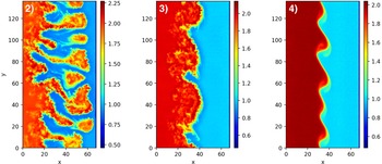
Since a velocity shear is present in simulations 2, 3 and 4, the onset of a KHI could be expected. Figure 6 shows the out-of-plane magnetic field at
 $t=350\unicode[STIX]{x1D714}_{ci}^{-1}$
for the three simulations with a velocity shear.
Magnetic field along
 $z$
at
 $t=350\unicode[STIX]{x1D714}_{ci}^{-1}$
for simulations 2, 3 and 4.

In simulation 4, where the LHDI does not develop, a series of KHI vortices forms. In simulation 3, despite the patchy layer produced by LHDI, the KHI dominates the large-scale nonlinear dynamics to form KHI vortices. Note that the fastest growing mode is different between simulations 3 and 4, despite having the same initial velocity shear and layer width. This is likely due to the widening of the initial shear layer induced by the LHDI in simulation 3. Finally, simulation 2 does not develop KH vortices. Nevertheless, the dynamics observed in simulation 2 is very similar to that of simulation 1 (which does not have a velocity shear – not plotted here), with only one difference that finger-like structures are drifting along
 $y$
in the former, while they do not in the latter. The nonlinear finger-like structures developed by the LHDI grow too quickly and reach the size of the expected KHI (black dashed line in figure 5) vortices long before the KHI could actually emerge. Thus, the layer coherence is long gone at the time where we would expect KHI. In simulation 2, the KHI has been killed by the nonlinear LHDI before it can develop.
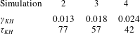
Now we try to estimate the growth rate of the fastest growing mode of the KHI, i.e.
 $\unicode[STIX]{x1D6FE}_{KH}$
, in all simulations with a velocity shear. In order to do that, we use the result of Michalke (Reference Michalke1964) (table 1 in the article): the fastest growing mode of the KHI over a layer with a hyperbolic tangent shape,
 $\tanh (x/L)$
, is given by
 $k_{KH}L=0.44$
, and
 $\unicode[STIX]{x1D6FE}_{KH}=0.095\unicode[STIX]{x0394}u/L$
. Such a result is obtained considering an incompressible fluid, in the absence of a magnetic field and with no density asymmetry. The incompressibility approximation roughly holds because the fast magnetosonic Mach number
 $M_{f}=u/\sqrt{c_{A}^{2}+c_{s}^{2}}$
(
 $c_{A}$
the Alfvén velocity and
 $c_{s}$
the sound velocity) is always smaller than 0.05 on both sides. We can however expect that minor compressibility effects would tend to slightly reduce the growth rate of the KHI in the above incompressible limit. Then, the presence of a magnetic field here also plays no relevant role because it is perpendicular to the propagation plane. Note however that the presence of a magnetic field gradient can also generate instabilities (Huba & Ossakow Reference Huba and Ossakow1980), but we neglect this term as we do not see any
 $\unicode[STIX]{x1D735}B$
-drift-induced instability in our simulations. Concerning the homogeneous density approximation, in general, we can expect that a density asymmetry
 $n_{r}$
would indeed alter the results of Michalke (Reference Michalke1964). However, following Chandrasekhar (Reference Chandrasekhar1961), we do expect that the growth rate would be modified as follows:
 $$\begin{eqnarray}\displaystyle \unicode[STIX]{x1D6FE}_{KH}\propto \frac{\sqrt{n_{r}}}{1+n_{r}}. & & \displaystyle\end{eqnarray}$$
In table 3, we have computed the growth rate for the KHI in the three simulations with the parameter
 $L$
computed at
 $t=10.0$
, when the linear growth of the LHDI is over. The width
 $L$
of the layer is calculated by fitting the profile of
 $v_{y}$
averaged along
 $y$
with (2.2), where
 $x_{0}$
and
 $L$
are left as free parameters. At this time, the layer width is more or less the same for all the simulations, corresponding to
 $L\sim 2$
. However, the layer width
 $L$
keeps growing slowly but continuously in simulations 2 and 3 because of the nonlinear LHDI. Thus, in practice, the KHI growth rate decreases with time in these simulations.
Theoretical growth rates
 $\unicode[STIX]{x1D6FE}_{KH}$
of the KHI for a layer width
 $L$
picked at
 $t=10$
;
 $\unicode[STIX]{x1D70F}_{KH}=1/\unicode[STIX]{x1D6FE}_{KH}$
is the characteristic time of the KHI growth.

The value of
 $\unicode[STIX]{x1D70F}_{KH}$
is calculated for simulation 4 with the method used in figure 5 (i.e. by fitting the curve of
 $\unicode[STIX]{x1D70E}_{0}(t)$
during its exponential growth, given that
 $\unicode[STIX]{x1D70E}_{0}$
is proportional to the KH wave amplitude) which gives us a result of
 $\unicode[STIX]{x1D70F}_{KH}\approx 49$
. Our theoretical
 $\unicode[STIX]{x1D70F}_{KH}$
is actually in good agreement with the observed one (42 versus 49), the slight discrepancy could be due to the error associated with
 $L$
, and the wave vector of maximum growth matches the one observed in the simulation
 $k=0.23$
. These results help us to clarify what is happening in the simulations.
In simulations 2 and 3 the LHDI grows much faster than the KHI, so we expect the LHDI to start the inverse-cascade process well before the KHI begins. Indeed, we see that the cascade begins at
 $t\sim 10$
and reaches fluid scales (
 $k\sim 1$
) at
 $t\sim 20$
. After that time the competition between the nonlinear LHDI and the KHI begins. In simulation 2,
 $\unicode[STIX]{x1D70F}_{NL}\ll \unicode[STIX]{x1D70F}_{KH}$
, so the nonlinear LHDI totally dominates the evolution and the KHI has no opportunity to grow. In simulation 3,
 $\unicode[STIX]{x1D70F}_{NL}\sim 2\unicode[STIX]{x1D70F}_{KH}$
so even if the nonlinear LHDI grows significantly, the KHI can still dominate. This case is interesting as both instabilities manage to develop sufficiently to impact the layer structure. In simulation 4 the LHDI is suppressed because there is no density gradient. So we see the formation of KHI vortices with a growth rate comparable to the one predicted by the theory.
4 Discussion
In this work we have shown that, despite the difference in characteristic scale lengths and growth rate values between the KHI and the LHDI, in the presence of a relatively strong density gradient the LHDI not only contributes to the dynamics but even dominates at large scales. The validity of these results and their application to space plasmas are discussed in this section.
In conditions of a boundary layer with both a velocity shear and a density gradient, the KHI and LHDI might compete. This competition relies on the linear time scales at which the instabilities develop and on the nonlinear time scale at which the layer diffuses and relaxes. All this can be summarized by three basic factors: the velocity shear amplitude, the density gradient amplitude and the layer width. When the importance of the density gradient dominates with respect to the velocity shear, then the structures generated during the nonlinear phase of the LHDI broaden, eventually smoothing the average velocity shear layer, thus slowing down (e.g. simulation 3) or even preventing (e.g. simulation 2) the KHI growth. A broadening of the layer then tends to decrease the growth rates of both KHI and LHDI. Moreover, for layers larger than a few ion inertial lengths, the LHDI growth rate rapidly decreases and eventually becomes stable. For example, with simulation 1 parameters, the LHDI becomes stable for
 $L\gtrsim 8$
. Therefore, when the velocity shear and the density gradient are characterized by nearly the same scale length, the layer width controls whether or not the LHDI develops. This is the reason why most planetary magnetopauses might be stable to the LHDI, as they are usually larger than a few ion inertial lengths, and why previous fully kinetic simulations of KHI in the Earth’s magnetopause did not see it (Matsumoto & Hoshino Reference Matsumoto and Hoshino2006; Umeda et al.
Reference Umeda, Miwa, Matsumoto, Nakamura, Togano, Fukazawa and Shinohara2010; Nakamura & Daughton Reference Nakamura and Daughton2014; Nakamura et al.
Reference Nakamura, Hasegawa, Daughton, Eriksson, Li and Nakamura2017). On the contrary, the Hermean magnetopause, characterized by a much smaller length scale of the boundary layer width, is potentially thin enough for the LHDI to develop and drive the dynamics, eventually inhibiting the KHI development. Such a study of KHI in the fully kinetic regime is therefore especially relevant for Mercury. As a matter of fact, simulation 2, which was designed with parameters expected in the magnetosphere of Mercury, shows that LHDI dominates the dynamics of such a strongly inhomogeneous shear layer.
The main topic of this study is the competition between the LHDI and the KHI in an inhomogeneous boundary layer and the LHDI nonlinear saturation. In this last phase, the mechanism behind the inverse cascade of the LHDI is out of the scope of this paper. However, it is worth recalling some previous results regarding the nonlinear phase of the LHDI concerning the inverse cascade (Davidson Reference Davidson1978; Huba, Gladd & Papadopoulos Reference Huba, Gladd and Papadopoulos1978; Gary & Sanderson Reference Gary and Sanderson1979; Brackbill et al. Reference Brackbill, Forslund, Quest and Winske1984; Drake et al. Reference Drake, Guzdar, Hassam and Huba1984; Shapiro et al. Reference Shapiro, Shevchenko, Cargill and Papadopoulos1994). On the one hand, the theory of Drake et al. (Reference Drake, Guzdar, Hassam and Huba1984), which relies on mode coupling to short-wavelength damped modes, works quite well in explaining the inverse cascade observed in this work. In particular, the temporal evolution of the spectra associated with the inverse cascade observed in our simulations is thoroughly described by Drake et al. (Reference Drake, Guzdar, Hassam and Huba1984). On the other hand, the modulational instability theory developed by Shapiro et al. (Reference Shapiro, Shevchenko, Cargill and Papadopoulos1994) might explain the exponential growth observed in the nonlinear phase of the LHDI (see figure 5). Moreover, Shapiro et al. (Reference Shapiro, Shevchenko, Cargill and Papadopoulos1994) predicted the formation of large-scale structures similar to those observed in our simulation at later times (see figure 6.1). These two explanations might be not exclusive.
For practical reasons linked to the full PIC modelling, our simulations use (i) a reduced mass ratio (ii) and a reduced geometry (two dimensions). Thus, the scale separation is much smaller than for a realistic mass ratio and it affects the LHDI development. Typically, the fastest growing mode of the LHDI in our simulations is for
 $k_{\text{FGM}}\sim 4$
, while for a realistic mass ratio it would been
 $k_{\text{FGM}}\sim 40$
(Gary Reference Gary1993). Drake et al. (Reference Drake, Guzdar, Hassam and Huba1984) argued that a realistic mass ratio will support the nonlinear evolution of the LHDI due to two reasons. First, the ratio of the rate of change of the magnetic field energy to particle drift energy scales as
 $m_{i}/m_{e}$
in a finite
 $\unicode[STIX]{x1D6FD}$
plasma (Drake, Gladd & Huba Reference Drake, Gladd and Huba1981), so much more energy will be available to supply the inverse cascade. Second, the number of unstable modes scales as
 $\sqrt{m_{i}/m_{e}}$
(Huba, Drake & Gladd Reference Huba, Drake and Gladd1980). So, for realistic values, we expect a much broader spectrum of unstable modes to be excited. For these reasons, we expect the LHDI nonlinear phase to develop faster for a realistic mass ratio as compared to our simulations. To support our claim, we observe that the growth of the nonlinear LHDI structures is faster than ours in the paper of Gary & Sgro (Reference Gary and Sgro1990), where the mass ratio is
 $m_{i}/m_{e}=100$
, despite a slightly smoother density gradient. Future studies will look at the impact of the mass ratio for realistic magnetopause parameters.
As this work has been performed in a reduced 2-D configuration, understanding the changes that would arise for a 3-D configuration in the linear and nonlinear development of the LHDI is a future necessary step. First of all, in three dimensions, the instability is no longer confined to the plane perpendicular to
 $B$
, so we expect growing modes with
 $\boldsymbol{k}\boldsymbol{\cdot }\boldsymbol{B}\neq 0$
. The nonlinear relaxation in three dimensions could lead to the formation of elongated cigar-shaped structures (Shapiro et al.
Reference Shapiro, Shevchenko, Cargill and Papadopoulos1994), to the acceleration of electrons parallel to the magnetic field (Singh & Leung Reference Singh and Leung1998; Bingham, Dawson & Shapiro Reference Bingham, Dawson and Shapiro2002) and to mode conversion towards different kinds of waves such as, e.g. whistler modes (Camporeale, Delzanno & Colestock Reference Camporeale, Delzanno and Colestock2012). How such effects would affect the competition and interaction between the LHDI and the KH is unclear and will be investigated in the future.
The work described in this paper highlights the importance of processes other than KHI to the generation of the large-scale structures responsible for plasma mixing along the magnetopause. In regions characterized by strong density inhomogeneities, such as the magnetopause of Mercury, the LHDI provides another efficient mechanism for plasma mixing, together with the KHI reported by MESSENGER observations (Slavin et al. Reference Slavin, Acuña, Anderson, Baker, Benna, Gloeckler, Gold, Ho, Killen and Korth2008). Some differences between the structures generated by KHI and LHDI should help us to identify them. Typically, during its late nonlinear phase, the KHI generates a diffuse layer (Matsumoto & Seki Reference Matsumoto and Seki2010), while the LHDI generates large-scale finger-like structures that do not evolve into a diffusive layer (Brackbill et al. Reference Brackbill, Forslund, Quest and Winske1984; Gary & Sgro Reference Gary and Sgro1990; Singh & Leung Reference Singh and Leung1998; Bingham et al. Reference Bingham, Dawson and Shapiro2002). Future studies should be dedicated to the interplay between KHI and LHDI structures in observations in order to understand the actual role of the LHDI in a Hermean-like magnetosphere. This requires observations at the lower-hybrid frequency, not available from MESSENGER data, but planned with the BepiColombo mission, especially with the PWI consortium onboard the Mio (MMO) spacecraft (Kasaba et al. Reference Kasaba, Bougeret, Blomberg, Kojima, Yagitani, Moncuquet, Trotignon, Chanteur, Kumamoto and Kasahara2010).
5 Conclusion
In this paper, we have performed several 2D-3V kinetic simulations (two spatial dimensions and three velocity dimensions) to study the linear and nonlinear evolution of a magnetized shear flow separating plasmas of different density and magnetic field intensity. This study shows that the large-scale structures that emerge from the nonlinear phase of the LHDI can interfere with the KHI development if the nonlinear LHDI driven dynamics modifies the velocity shear layer. In a layer subjected to both a velocity shear and a density gradient, we have shown that, at early times and within the parameter range used in this study, a LHDI develops first. Then, the LHDI enters a nonlinear phase and energy starts to cascade from small to large scales. Depending on the growth rate of those structures, the system can become totally dominated by the nonlinear LHDI and the KHI will not be able to develop. On the contrary, if the nonlinear LHDI growth rate is smaller than the KHI growth rate, the KHI dominates and leads to the formation of vortices. However, those vortices are already partially mixed due to the simultaneous, if less efficient, development of the LHDI at smaller scales.
The range of parameters used in this study encompasses those expected in the magnetosphere of Mercury (e.g. simulation 2). We therefore expect that these kind of structures could be detected by future observations provided by the BepiColombo space mission.
Acknowledgements
This project (J.D., F.C.) has received funding from the European Union’s Horizon 2020 research and innovation programme under grant agreement no. 776262 (AIDA). We acknowledge ISCRA for awarding us access to the supercomputer Marconi at CINECA, Italy, where the calculations were performed. We thank M. Guarrasi (CINECA) for useful discussion about code implementation on Marconi. The work at LPC2E/CNRS was supported by CNES and by ANR under the financial agreement ANR-15-CE31-0009-01. The work by F.P. has been supported by Fonds Wetenschappelijk Onderzoek - Vlaanderen (FWO) through the postdoctoral fellowship 12X0319N. S.S.C. is supported by the National Aeronautics and Space Administration under Grant no. NNX16AK09G issued through the Heliophysics Supporting Research Program.
Supplementary movies
Supplementary movies are available at https://doi.org/10.1017/S0022377819000758.