2.1 Growth

Let M be a (not necessarily inverse) monoid generated (as a monoid) by a finite set X. Recall that the length of an element $m \in M$ is the smallest k such that M can be written as a word of length k over the generating set X. For $K \in \mathbb {N}$ the sphere of radius K is the set of elements in M of length exactly K, and it is denoted by $S(K)$ . The (spherical) growth function of M (with respect to X) is the function $\gamma \colon \mathbb {N} \to \mathbb {N}$ defined by $K \mapsto |S(K)|$ . The (exponential) growth rate of M is defined to be the asymptotic exponential growth rate of the function $\gamma $ , that is,

(2) $$ \begin{align} \limsup_{n \to \infty} \gamma(n)^{\frac{1}{n}}. \end{align} $$

Since the growth rate is submultiplicative, i.e. $\gamma (m+n) \leq \gamma (m)\gamma (n)$ for all $m, n \in {\mathbb {N}}$ , the limit (2) always exists. If the limit (2) is greater than $1$ , then M is said to have exponential growth. If there are natural numbers $C, d \in {\mathbb {N}}$ such that $\gamma (n) \leq (Cn)^d$ for all $n \in {\mathbb {N}}$ , then we say that M has polynomial growth (of degree d, where d is the smallest such). All growth in this article, with the sole exception of the monogenic free inverse monoid treated in §3.4 (see Proposition 3.4), will be exponential.

2.2 Free inverse monoids

Inverse monoids form a variety of algebras, and thus free inverse monoids exist; see [Reference LawsonLaw98, Chapter 6, §1]. We denote the free inverse monoid on X by $\operatorname {\mathrm {FIM}}(X)$ , and $|X|$ is called the rank of $\operatorname {\mathrm {FIM}}(X)$ . Then $\operatorname {\mathrm {FIM}}(X)$ is generated as a monoid by $X \cup X^{-1}$ , where $X^{-1}$ is a set in bijective correspondence with X and such that $X \cap X^{-1} = \varnothing $ , and we will study its growth with respect to this generating set. If $|X|= k$ , we shall sometimes write $\operatorname {\mathrm {FIM}}_k$ for $\operatorname {\mathrm {FIM}}(X)$ , and call this the free inverse monoid of rank k. Free inverse monoids have many peculiar properties differentiating them from free groups. For example, Schein [Reference ScheinSch75] proved that $\operatorname {\mathrm {FIM}}_k$ is not finitely presented as a monoid, even when $k=1$ (although it is finitely generated). Indeed, $\operatorname {\mathrm {FIM}}_1$ does not have the homological finiteness property $\operatorname {FP}_2$ (and hence neither does any $\operatorname {\mathrm {FIM}}_k$ for $k \geq 1$ ), a strictly weaker property than finite presentability [Reference Gray and SteinbergGS21]. Neither does the analogue of the Nielsen–Schreier Theorem hold for $\operatorname {\mathrm {FIM}}_k$ : there exist non-free inverse submonoids of $\operatorname {\mathrm {FIM}}_k$ , see [Reference ReillyRei72]. Even solving the word problem in $\operatorname {\mathrm {FIM}}_k$ is a non-trivial task, see [Reference ScheiblichSch73, Reference MunnMun74]; this is normally done via Munn trees, which we now define.

2.3 Munn trees

The model of free inverse monoids most commonly used in semigroup theory is due to Munn [Reference MunnMun74], which we briefly recall. This represents elements of $\operatorname {\mathrm {FIM}}(X)$ as birooted trees called Munn trees, and also provides a compelling link between $\operatorname {\mathrm {FIM}}(X)$ and the Cayley graph $\Gamma _X$ of the free group $\operatorname {\mathrm {FG}}(X)$ . Elements of $\operatorname {\mathrm {FIM}}(X)$ are uniquely represented by the pairs $(T,g)$ , where T is a connected subgraph (and thus a subtree) of $\Gamma _X$ containing the vertex $1$ , and g is a vertex of T. The product of two Munn trees $(T_1,g_1)$ and $(T_2,g_2)$ is $(T_1 \cup g_1\cdot T_2, g_1g_2)$ , where $g_1\cdot T_2$ denotes the image of $T_2$ under the left action of $g_1$ . The Munn tree corresponding to a generator $x \in X \cup X^{-1}$ is the pair $(\langle x \rangle , x)$ where $\langle x \rangle $ is the subgraph of $\Gamma _X$ spanned by the unique edge that x labels from $1$ . It follows that the Munn tree represented by a product $w \in (X \cup X^{-1})^\ast $ of generators is the pair $(\langle w \rangle , w_{\operatorname {\mathrm {FG}}(X)})$ where $\langle w \rangle $ is the subgraph of $\Gamma _X$ spanned by the unique path that w labels from $1$ , and $w_{\operatorname {\mathrm {FG}}(X)}$ is the element of $\operatorname {\mathrm {FG}}(X)$ represented by w (i.e. its freely reduced form), which is also the terminal vertex of this path. Clearly, a Munn tree $(T,g)$ is idempotent if and only if $g=1$ .

2.4 Growth of inverse monoids

The growth rate of the free inverse monoid of rank r is also automatically an upper bound on the growth rate of any r-generated inverse monoid or semigroup, since there is always a surjective homomorphism from $\operatorname {\mathrm {FIM}}_r$ onto any r-generated inverse monoid. The growth of different classes of inverse monoids has been studied, and although we cannot hope to survey this subject in its entirety here, there are many tantalizing open problems in this area. For example, classifying precisely what the growth of one-relation inverse monoids can be remains an open problem, cf. [Reference ShneersonShn15, p. 235]. Furthermore, Shneerson & Easdown [Reference Shneerson and EasdownSE11] have studied the growth of certain Rees quotients of free inverse monoids; in [Reference Easdown and ShneersonES13] the same authors give sufficient conditions for a one-relation inverse monoid, i.e. the quotient of $\operatorname {\mathrm {FIM}}(X)$ by some relation $w_1 = w_2$ , to have exponential growth. One such sufficient condition is that $|X|=2$ and that the Munn trees of both $w_1$ and $w_2$ contain more than one edge. One natural direction for future research would be to investigate the precise exponential growth rates in these cases: in particular, whether they are always algebraic numbers, as for $\operatorname {\mathrm {FIM}}(X)$ (as we shall prove in Theorem 5.5). We also remark that methods arising from growth were used by Cutting & Solomon [Reference Cutting and SolomonCS01] to show that $\operatorname {\mathrm {FIM}}_1$ is not automatic (and hence neither is $\operatorname {\mathrm {FIM}}_r$ for $r \geq 1$ ), and indeed does not admit a regular language of normal forms.

3.1 Tree diagrams of branching $(p,q)$

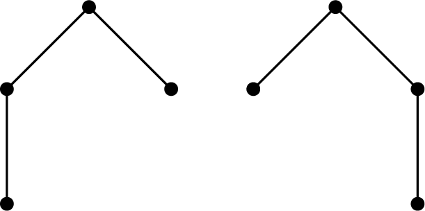
Consider the infinite rooted (undirected) tree $T_{p,q}$ where the root has q children and all other vertices have p children. The finite subtrees containing the root are called tree diagrams with branching (p,q) – these are rooted trees where the root has at most q children, and all other vertices have at most p children, but considered as subgraphs of the infinite tree rather than up to isomorphism; for example, the two graphs in Figure 1 are two distinct tree diagrams with branching $(1,2)$ . For $p=q$ , we simply say tree diagrams with branching p. Of particular importance to us are the p-ary tree diagrams, which are those tree diagrams with branching p where every internal node has exactly p children.

Figure 1

Two distinct tree diagrams with branching $(1,2)$ .

The Fuss-Catalan numbers $R_{p,q}(k)$ are the numbers defined (cf. [Reference Beagley and DrubeBD15, Theorem 2.5]) by the formula

$$\begin{align*}R_{p,q}(k)=\frac{q}{kp+q} \binom{kp+q}{k}=\frac{q}{k} \binom {kp+q-1}{k-1}. \end{align*}$$

Fuss-Catalan numbers are important for us because they count tree diagrams of branching $(p,q)$ ; we believe this fact to be folklore, but include a proof as we have been unable to find a reference.

Proof. Let $D_{p,q}(k)$ denote the number of tree diagrams with branching $(p,q)$ on k edges. We show that $D_{p,q}(k)$ satisfies the same recursion as $R_{p,q}(k)$ . By [Reference Beagley and DrubeBD15, Lemma 2.4], $R_{p,q}(k)$ satisfies the equation

$$\begin{align*}R_{p,q}(k)=\sum_{\substack{i_1+\cdots+i_q=k \\ i_1, \dots, i_q \geq 0}} {}_pc_{i_1}\cdots {}_pc_{i_q}, \end{align*}$$

where $_pc_i$ denotes the ith p-Catalan number, and where $p\geq 1$ and $i \geq 0$ .

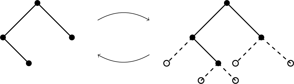
The p-Catalan numbers, also called the generalized Catalan numbers, have been widely studied. In particular (see e.g. [Reference Hilton and PedersenHP91, Theorem 0.2]), the number $_pc_i$ is equal to the number of p-ary tree diagrams with i internal nodes. We claim that these are in bijection with the set of tree diagrams with branching p on i nodes, together with the empty set. Indeed, if T is any tree diagram with branching p on i nodes, it can be turned into a p-ary tree with i internal nodes by completing all i nodes to have p children, and conversely, deleting all leaves from a p-ary tree diagram with $i \geq 1$ internal nodes gives a tree diagram with branching p on i nodes; see Figure 2. The single p-ary tree diagram with $i=0$ internal nodes is the tree diagram consisting of a single vertex, and this corresponds to the empty set under this bijection.

Figure 2

The bijection taking a tree diagram with branching 2 on 4 nodes to a 2-ary tree diagram with 4 internal nodes.

Let us count the number $D_{p,q}(k)$ of tree diagrams with branching $(p,q)$ on k edges. Let $T \subseteq T_{p,q}$ be such a tree diagram, and for all $1\leq j \leq q$ , consider the subtree $T^j_{p,q}$ of $T_{p,q}$ induced on all descendants of the jth vertex of level one. Define $T_j=T^j_{p,q} \cap T$ – this is either a tree diagram with branching p, or empty. Notice that T is uniquely determined by the tuple $(T_1, \ldots , T_q)$ . Every node of T but the root is contained in exactly one of the subtrees $T_j$ , which gives $V(T)=V(T_1)+\ldots +V(T_q)+1$ , hence $k=V(T)-1=V(T_1)+\ldots +V(T_q)$ . Thus $D_{p,q}(k)$ is equal to the number of q-tuples $(T_1, \ldots , T_q)$ where each $T_j$ is either a tree diagram with branching p, or empty, and where $V(T_1)+\ldots +V(T_q)=k$ . The number of such tuples is exactly $\displaystyle \sum _{i_1+\cdots +i_q=k} {}_pc_{i_1}\cdots {}_pc_{i_q}$ as needed.

We are now ready to use these combinatorial results to count Munn trees, and by extension also enumerate the spheres of a given radius in $\operatorname {\mathrm {FIM}}(X)$ .

3.2 Counting Munn trees

Let $(T,g) \in \operatorname {\mathrm {FIM}}(X)$ be a Munn tree. The length of $(T,g)$ can be expressed directly in terms of trunk edges and branch edges, as follows.

Consider the set of all Munn trees with a given trunk. That is, fix $g \in \operatorname {\mathrm {FG}}(X)$ and consider the set $\{ (T,g) : T \ \mathrm{is \ a \ subtree \ in \ the \ Cayley \ graph }\ \Gamma _X \ \mathrm{containing }\ 1\ \mathrm{ and }\ g \}$ . Let w be the unique freely reduced word representing g, and assume w has length t. Let $p_w$ denote the path in $\Gamma _X$ from $1$ to g which is labelled by w. This path is then the common trunk of all Munn trees $(T,g)$ .

Consider the graph obtained from $\Gamma _X$ by contracting $p_w$ into a single vertex $\alpha $ . Notice that this graph is a tree where every vertex except $\alpha $ has valence $2|X|$ . Consider it as a rooted tree with root $\alpha $ . Notice that Munn trees with trunk $p_w$ are in bijection with the finite, rooted subtrees of this infinite rooted tree, which are in turn counted by Fuss-Catalan numbers. All that remains is to determine the valence of $\alpha $ – this will depend on the length t of the trunk. A vertex in the contracted graph is adjacent to $\alpha $ if its preimage in $\Gamma _X$ was adjacent to a vertex of $p_w$ , so it suffices to count how many such vertices there were. In $\Gamma _X$ , every vertex has degree $2|X|$ , so if w is not the empty word, then any internal node of the trunk will connect to exactly $2|X|-2$ vertices of $\Gamma _X$ which do not lie on the trunk, and the endpoints $1$ and g of the trunk connect to $2|X|-1$ vertices not on the trunk. Since there are $t-1 \geq 0$ internal nodes, the number of such vertices is $2(2|X|-1)+(t-1)(2|X|-2)$ . If w is the empty word, that is, if $t-1=-1$ , then the trunk consists of a single vertex $1$ and it has $2|X|$ neighbours. Thus, $\alpha $ always has valence $2(2|X|-1)+(t-1)(2|X|-2)$ .

It follows that $\alpha $ has exactly $2(2|X|-1)+(t-1)(2|X|-2)$ children, while all non-root vertices in the contracted tree have exactly $2|X|-1$ children. Putting $p=2|X|-1$ and $q=2p+(t-1)(p-1)$ , this tree is therefore exactly $T_{p,q}$ , and the set of all Munn trees with trunk $p_w$ are counted by $R_{p,q}(k)$ exactly. Thus, we have proved:

Let $M(t,k)$ denote the set of Munn trees with t trunk edges and k branch edges. Taking notation as in Lemma 3.3, it follows from the same lemma that

$$\begin{align*}|M(t,k)|=R_{p,q}(k) \cdot|\{w \in (X \cup X^{-1})^*\ \mathrm{ is \ a \ freely \ reduced \ word \ of \ length}\ t\}|, \end{align*}$$

since the second factor in the above expression is the number of possible fixed trunks of length t. If $t\geq 1$ , then there are $(p+1)p^{t-1}$ possible freely reduced words of length t (we have $p+1$ choices for the first letter, and p for the rest), and there is one reduced word of length $0$ . For any $t \geq 1$ , this gives the formula

(3) $$ \begin{align} |M(t,k)| & = (p+1)p^{t-1}R_{p,2p+(t-1)(p-1)}(k)=\nonumber \\ &=(p+1)p^{t-1}\frac{2p+(t-1)(p-1)}{kp+2p+(t-1)(p-1)} \binom{kp+2p+(t-1)(p-1)}{k}, \end{align} $$

and the particular case of $t=0$ becomes

(4) $$ \begin{align} |M(0,k)|=R_{p,p-1}(k) = \frac{p+1}{kp+p+1} \binom{kp+p+1}{k}. \end{align} $$

Thus, we have counted the number of Munn trees $M(t,k)$ of a given number t of trunk edges and k of branch edges.

3.3 Sphere size

Using the results of §3.2, it is now straightforward to calculate the size $|S(K)|$ of the sphere of radius K in $\operatorname {\mathrm {FIM}}(X)$ . Any Munn tree in $M(t,k)$ has length $t+2k$ by Lemma 3.2. In particular, idempotents (being exactly those Munn trees with trunk length $0$ ) always have an even length. If K is even, then

(5) $$ \begin{align} \begin{aligned} |S(K)|&= |M(0,\frac{1}{2}K)|+\sum_{\substack{t+2k = K \\ t \geq 1, \ k \geq 0}}|M(t,k)|=\\ &=\frac{p+1}{\frac{1}{2} Kp+p+1} \binom{\frac{1}{2}Kp+p+1}{\frac{1}{2}K}+\\ & + \sum_{\substack{t+2k = K \\ t \geq 1, \ k \geq 0}}(p+1)p^{t-1}\frac{2p+(t-1)(p-1)}{kp+2p+(t-1)(p-1)} \binom{kp+2p+(t-1)(p-1)}{k}, \end{aligned} \end{align} $$

and when K is odd, we have

(6) $$ \begin{align} \begin{aligned} |S(K)|&=\sum_{\substack{t+2k = K \\ t \geq 1, \ k \geq 0}}|M(t,k)|=\\ &=\sum_{\substack{t+2k= K\\ t \geq 1, \ k \geq 0}}(p+1)p^{t-1}\frac{2p+(t-1)(p-1)}{kp+2p+(t-1)(p-1)} \binom{kp+2p+(t-1)(p-1)}{k}. \end{aligned} \end{align} $$

By a simple summation, one could also of course deduce corresponding formulae for the size of the ball of a given radius.

3.4 The monogenic case

Before embarking on an in-depth analysis of the asymptotics of (5) and (6) for $|X|>1$ , we consider the much easier monogenic case, i.e. when $|X| = 1$ . In this case, $p=1$ and (3) simplifies to give

$$\begin{align*}M(t,k) = 2 \frac{p+1}{kp+p+1} \binom{kp+p+1}{k}= 2 \frac{2}{k+2} \binom{k+2}{k}=2k+2, \end{align*}$$

for $t \geq 1$ which makes

$$\begin{align*}|S(2R+1)|=\sum_{\substack{t+2k= 2R+1 \\ t \geq 1, \ k \geq 0}} 2k+2=\sum_{k=0}^R 2k+2=R^2+3R+2,\end{align*}$$

and, almost identically, we have

$$\begin{align*}|S(2R)|=R+1+\sum_{\substack{t+2k= 2R\\ t \geq 1, \ k \geq 0}} 2k+2=R+1+\sum_{k=0}^{R-1} 2k+2=R^2+2R+1. \end{align*}$$

Thus, we obtain the following well-known (cf. e.g. [Reference Shneerson and EasdownSE96] and [Reference Cutting and SolomonCS01, Theorem 2.4]) result:

We will now expand in two directions; first, in §4 we use (4) to find a formula for the growth rate of the number of idempotents in $\operatorname {\mathrm {FIM}}(X)$ in Theorem 4.1. Next, in §5, we will analyze the formulae (5) and (6) in depth to find the exponential growth rate of $\operatorname {\mathrm {FIM}}(X)$ when $|X|>1$ in Theorem 5.5.

5.1 Roots of polynomials

We shall need the following elementary fact.

Now we use Lemma 5.1 to determine the behaviour of the maximal roots of a certain family of polynomials. These roots will be the exponential growth rates of the free inverse monoids, as we will see in Theorem 5.5.

Lemma 5.2. Let $p\in \mathbb {N}$ with $p \geq 2$ . Let $y=y(p)$ be the largest real solution to $p^p y^{p-2} - (py-1)^{p-1}=0$ . Then $y\in (p,p+1)$ and, as $p \to \infty $ , we have

(8) $$ \begin{align} y=p+1-\frac{3}{2p}+o\left( \frac{1}{p} \right). \end{align} $$

Proof. We divide the polynomial equation throughout by $p^{2p-2}$ to obtain

$$ \begin{align*} \left( \frac{y}{p} \right) ^{p-2} = \left( \frac{y}{p} - \frac{1}{p^2}\right)^{p-1}. \end{align*} $$

We will write $z=y/p$ . The plan now is to justify that this has a root $z\in (1,1+1/p)$ by using the intermediate value theorem applied to the following polynomial:

$$ \begin{align*} f(z)=\left( z- \frac{1}{p^2} \right)^{p-1} - z^{p-2}. \end{align*} $$

It is easy to see that $f(1)<0$ . Therefore it now suffices for us to show that $f(1+1/p)>0$ . This is straightforward to verify when $p=2$ , so instead assume $p\geq 3$ . We use the binomial expansion to obtain

$$ \begin{align*} f(z)=z^{p-1}-z^{p-2} - (p-1)\frac{z^{p-2}}{p^2} + \frac{(p-1)(p-2)}{2} \frac{z^{p-3}}{p^4} + \sum_{i=3}^{p-1}(-1)^i{ p-1 \choose i } \frac{z^{p-1-i}}{p^{2i}}, \end{align*} $$

where the rightmost summation is taken to be $0$ in the case $p=3$ . This can be written as

$$ \begin{align*} f(z)=z^{p-3}\left[ z\left( z-1-\frac{1}{p}+\frac{1}{p^2}\right) +\frac{(p-1)(p-2)}{2p^4} \right] + \sum_{i=3}^{p-1}(-1)^i{ p-1 \choose i } \frac{z^{p-1-i}}{p^{2i}}. \end{align*} $$

From now on assume $z>1$ . By dividing throughout by $z^{p-3}$ , we find that

(9) $$ \begin{align} \frac{f(z)}{z^{p-3}} = \left[ z\left( z-1-\frac{1}{p}+\frac{1}{p^2}\right) +\frac{(p-1)(p-2)}{2p^4} \right] + \sum_{i=3}^{p-1}(-1)^i{ p-1 \choose i } \frac{z^{2-i}}{p^{2i}}, \end{align} $$

and hence

$$ \begin{align*} \frac{f(z)}{z^{p-3}} \geq \left[ z\left( z-1-\frac{1}{p}+\frac{1}{p^2}\right) +\frac{(p-1)(p-2)}{2p^4} \right] - \sum_{\substack{i \ \mathrm{odd}\\ i=3}}^{p-1}{ p-1 \choose i } \frac{z^{2-i}}{p^{2i}}. \end{align*} $$

Since ${p-1 \choose i}$ is bounded from above by $p^i$ we have

$$ \begin{align*} \frac{f(z)}{z^{p-3}} \geq \left[ z\left( z-1-\frac{1}{p}+\frac{1}{p^2}\right) +\frac{(p-1)(p-2)}{2p^4} \right] - \sum_{\substack{i \ \mathrm{odd}\\ i=3}}^{p-1}p^i \frac{z^{2-i}}{p^{2i}}. \end{align*} $$

Notice that the summation in the final term can be manipulated to obtain

$$ \begin{align*} - \sum_{\substack{i \ \mathrm{odd}\\ i=3}}^{p-1}p^i \frac{z^{2-i}}{p^{2i}}>- (z^{-1}p^{-3}+z^{-3}p^{-5}+z^{-5}p^{-7}+ \cdots ) = - \frac{1}{zp^3 \left(1-\frac{1}{z^2p^2}\right)}. \end{align*} $$

Hence for all $z>1$

$$ \begin{align*} \frac{f(z)}{z^{p-3}}>\left[ z\left( z-1-\frac{1}{p}+\frac{1}{p^2}\right) +\frac{(p-1)(p-2)}{2p^4} \right] - \frac{1}{zp^3 \left(1-\frac{1}{z^2p^2}\right)}. \end{align*} $$

Now substituting in $z=1+\frac {1}{p}$ , we get

$$ \begin{align*} \frac{f(1+\frac{1}{p})}{(1+\frac{1}{p})^{p-3}}>\left[ \frac{3}{2p^2}-\frac{1}{2p^3} +\frac{1}{p^4} \right] - {\frac{1}{zp^3 \left(1-\frac{1}{z^2p^2}\right)}}, \end{align*} $$

where the rightmost denominator is

$$ \begin{align*} zp^3 \left(1-\frac{1}{z^2p^2}\right)=(p^3+p^2)\left(1-\frac{1}{p^2+2p+1}\right)> p^3, \end{align*} $$

from which it follows that

$$ \begin{align*} \frac{f(1+\frac{1}{p})}{(1+\frac{1}{p})^{p-3}}> \left[ \frac{3}{2p^2}-\frac{1}{2p^3} +\frac{1}{p^4} \right]-\frac{1}{p^3} > \frac{1}{p^4}>0. \end{align*} $$

Thus, we have proved that $f(1+\frac {1}{p})>0$ . Since $f(1)<0$ , by the intermediate value theorem there is a root $z\in (1,1+1/p)$ and as $z = y/p$ , there is a root $y\in (p,p+1)$ as claimed. Hence, by Lemma 5.1 (applied with $t=py$ ) the root y is the maximal root of our polynomial because it is the unique root in the interval $(\frac {1}{p},\infty )$ .

We now prove the asymptotic formula (8) as $p\rightarrow \infty $ . Let z be the unique root of $f(z)$ in the interval $(1, 1+\frac {1}{p})$ , and set $z=1+1/p+C/p^2$ – note that C depends on p, and $-p < C < 0$ . Substitute this formula for z into (9). Elementary algebraic manipulations then yield

$$ \begin{align*} 0=\frac{f(z)}{z^{p-3}}=\left[ \frac{2C+3}{2p^2} +\frac{2C-1}{2p^3}+\frac{C^2 +C +1}{p^4} \right] + \sum_{i=3}^{p-1}(-1)^i{ p-1 \choose i } \frac{z^{2-i}}{p^{2i}}. \end{align*} $$

Note that since $z>1$ by assumption, we have $z^{2-i} < 1$ whenever $i \geq 3$ , and thus

$$ \begin{align*} \left|\sum_{i=3}^{p-1}(-1)^i{ p-1 \choose i } \frac{z^{2-i}}{p^{2i}}\right|&\leq \sum_{i=3}^{p-1}{ p-1 \choose i } \frac{z^{2-i}}{p^{2i}} \leq \sum_{i=3}^{p-1}{ p-1 \choose i } \frac{1}{p^{2i}} \\ &\leq \sum_{i=3}^{p-1} \frac{1}{p^{i}} \leq \frac{1}{p^3} + \frac{p-5}{p^4} < \frac{2}{p^3}. \end{align*} $$

Furthermore, since $|C|\leq p$ , we have that

$$ \begin{align*}\left|\frac{2C-1}{2p^3}+\frac{C^2 +C +1}{p^4}\right|\leq \frac{2|C|+|1|}{2p^3}+\frac{|C^2| +|C| +|1|}{p^4} < \frac{5}{p^2}. \end{align*} $$

Therefore as $p\rightarrow \infty $ , we get

$$ \begin{align*} 0= \frac{f(z)}{z^{p-3}} = \frac{2C+3}{2p^2} +O\left( \frac{1}{p^2}\right), \end{align*} $$

in particular, $0=2C+3+O(1),$ that is, $C=-3/2+O(1)$ and therefore C is bounded. This allows us to refine the estimations above and observe that $\frac {2C-1}{2p^3}+\frac {C^2 +C +1}{p^4}$ is also $o(1/p^2)$ , hence

$$ \begin{align*} 0= \frac{f(z)}{z^{p-3}} = \frac{2C+3}{2p^2} +o\left( \frac{1}{p^2}\right), \end{align*} $$

which yields $C=-3/2+o(1)$ . Substituting this into $z=1+1/p+C/p^2$ , we obtain that the unique root for the polynomial $f(z)$ , where $z=y/p$ , is $1+1/p-3/(2p^2)+o(1/p^2)$ . This proves (8).

5.2 Exponential growth of free inverse monoids

We will now use the sizes of the spheres determined in §3 to determine the exponential growth rate of $\operatorname {\mathrm {FIM}}_r$ when $r>1$ .

Recall that the growth rate is defined as

$$\begin{align*}\limsup_{K\rightarrow\infty} \left( |S(K)| \right)^{\frac{1}{K}}. \end{align*}$$

There are only polynomially many terms in our formulae (5) and (6) for $|S(K)|$ with respect to K, so the exponential growth rate y is determined by the growth rate of the sequence of maximal terms. Moreover, by Theorem 4.1, the exponential growth rate of the idempotents is strictly less than $2 |X| -1$ , which is a lower bound on the exponential growth rate of $\operatorname {\mathrm {FIM}}(X)$ , so the term (which occurs in the even case only) corresponding to trunk length $0$ may be ignored. Thus the growth rate is equal to

(10) $$ \begin{align} \limsup_{K\rightarrow \infty} \max_{\substack{t+2k= K\\ t \geq 1, k \geq 0}} |M(t, k)|^{\frac{1}{K}}. \end{align} $$

Clearly we can choose a sequence of values $t_i, k_i$ and $K_i$ for $t, k$ and K respectively such that the limit $\lim _{i \to \infty }|M(t_i, k_i)|^{\frac {1}{K_i}}$ of the corresponding terms converges to the growth rate. We begin with a lemma which will help us identify key properties of the sequences $t_i, k_i$ .

Lemma 5.3. Let $K_i$ , $t_i$ and $k_i$ ( $i \in {\mathbb {N}}$ ) be non-negative integer sequences such that $t_i \geq 1$ , $K_i = t_i + 2k_i$ , and $K_i \to \infty $ as $i \to \infty $ . Assume furthermore that

$$\begin{align*}y = \lim_{i \to \infty} M(t_i, k_i)^{\frac{1}{K_i}} \end{align*}$$

is defined and finite, where $M(t_i, k_i)$ denotes the set of Munn trees over the alphabet X with $t_i$ trunk edges and $k_i$ branch edges as in §3. If as $i \to \infty $ either $k_i$ is bounded above or $\frac {t_i-1}{k_i}$ is not bounded above, then $y \leq p$ . Otherwise, if x is any accumulation point of the sequence $\frac {t_i-1}{k_i}$ , then

(11) $$ \begin{align} y = \exp \frac{1}{x+2} \bigg( x\log (p)+ \left( p+ x(p-1) \right) \log \left( p+ x(p-1) \right) \nonumber \\ - \left( (p-1) + x(p-1) \right) \log \left( (p-1) + x(p-1) \right) \bigg). \end{align} $$

Proof. By (3) we have

(12) $$ \begin{align} y & =\lim_{i\rightarrow \infty} \left( (p+1)p^{t_i-1}\frac{2p+(t_i-1)(p-1)}{k_ip+2p+(t_i-1)(p-1)} \binom{k_ip+2p+(t_i-1)(p-1)}{k_i}\right)^{ \frac{1}{K_i}} \nonumber \\ & =\lim_{i\rightarrow \infty}\underbrace{ \left( (p+1)\frac{2p+(t_i-1)(p-1)}{k_ip+2p+(t_i-1)(p-1)} \right)^{ \frac{1}{K_i}}}_{\to 1 \text{ as } i \to \infty} \left( p^{t_i-1} \binom{k_ip+2p+(t_i-1)(p-1)}{k_i}\right)^{ \frac{1}{K_i}} \nonumber \\ & =\lim_{i\rightarrow \infty} \left( p^{t_i-1} \binom{k_ip+2p+(t_i-1)(p-1)}{k_i}\right)^{ \frac{1}{K_i}}. \end{align} $$

Suppose first that the sequence $k_i$ is bounded above by some constant B. Then, since $\binom {n}{r} \leq n^r$ , we can bound the last term in (12), yielding

$$ \begin{align*} y \leq \lim_{i\rightarrow \infty} \left( p^{t_i-1} \right)^{\frac{1}{K_i}} \underbrace{\left( (Bp+2p+(t_i-1)(p-1))^B \right)^{\frac{1}{K_i}}}_{\to 1 \text{ as } i \to \infty} = \lim_{i\rightarrow \infty} \left( p^{t_i-1} \right)^{\frac{1}{K_i}} \leq p, \end{align*} $$

where the final inequality is due to the fact that $t_i \leq K_i$ for all i. Thus, the claim is proved in the case where $k_i$ is uniformly bounded above, so assume that it is not.

In this case, by passing to a subsequence if necessary, we may assume that $k_i \to \infty $ as $i \to \infty $ . Hence the three sequences $k_ip+2p+(t_i-1)(p-1)$ , $k_i$ , and $k_i(p-1)+2p+(t_i-1)(p-1)$ , all tend to infinity as $i \to \infty $ . Thus, we may use Stirling’s approximation for each of these three sequences to replace

$$\begin{align*}\binom{k_ip+2p+(t_i-1)(p-1)}{k_i} \end{align*}$$

in (12) by the expression

$$\begin{align*}\frac{ (k_ip+2p+(t_i-1)(p-1))^{k_ip+2p+(t_i-1)(p-1)}}{k_i^{k_i}{(k_i(p-1)+2p+(t_i-1)(p-1))^{k_i(p-1)+2p+(t_i-1)(p-1)}}} \alpha(t_i,k_i) \end{align*}$$

where $\alpha $ is a rational function of the $t_i$ and $k_i$ such that $\alpha (t_i, k_i)^{\frac {1}{K_i}} \to 1$ as $i \to \infty $ . Doing this substitution into (12) thus eliminates the $\alpha (t_i, k_i)$ in the limit, and we are left to analyze

$$\begin{align*}y =\lim_{i\rightarrow \infty} \left( p^{t_i-1} \frac{ (k_ip+2p+(t_i-1)(p-1))^{k_ip+2p+(t_i-1)(p-1)}}{k_i^{k_i}{(k_i(p-1)+2p+(t_i-1)(p-1))^{k_i(p-1)+2p+(t_i-1)(p-1)}}}\right)^{ \frac{1}{K_i}}. \end{align*}$$

From this point on, for ease of calculation, we set $n_i = t_i-1$ so that $K_i = t_i + 2 k_i = n_i + 1 + 2 k_i$ and take logarithms, yielding

(13) $$ \begin{align} y = \lim_{i\rightarrow\infty} \exp \frac{1}{n_i+1+2k_i}\left( n_i \log(p) +\log Q(p, n_i, k_i) \right), \end{align} $$

where we have set

$$\begin{align*}Q(p, n_i, k_i) = \frac{ (k_ip+2p+n_i(p-1))^{k_ip+2p+n_i(p-1)}}{k_i^{k_i}{(k_i(p-1)+2p+n_i(p-1))^{k_i(p-1)+2p+n_i(p-1)}}}. \end{align*}$$

Dividing the numerator and denominator of $Q(p, n_i,k_i)$ by $k_i^{k_ip + 2p + n_i(p-1)}$ , then factoring out $k_i$ factors from all exponents, we obtain

(14) $$ \begin{align} \log Q(p, n_i, k_i) = k_i \log \frac{\left(p + \frac{2p}{k_i} + \frac{n_i}{k_i}(p-1)\right)^{p + \frac{2p}{k_i} + \frac{n_i}{k_i}(p-1)}}{\left( p-1 + \frac{2p}{k_i} + \frac{n_i}{k_i}(p-1)\right)^{p-1 + \frac{2p}{k_i} + \frac{n_i}{k_i}(p-1)}}. \end{align} $$

By using the properties of logarithmic functions, we can rewrite (14) as

(15) $$ \begin{align} \log Q(p, n_i, k_i) &= k_i \left[ \left( p + \frac{2p}{k_i} + \frac{n_i}{k_i} (p-1) \right) \log \left( p + \frac{2p}{k_i} + \frac{n_i}{k_i} (p-1) \right) \nonumber \right. \\ &\quad\left. - \left( p-1 + \frac{2p}{k_i} + \frac{n_i}{k_i}(p-1) \right) \log\left(p-1 + \frac{2p}{k_i} + \frac{n_i}{k_i}(p-1)\right)\right]. \end{align} $$

Now, using the simple equality

$$\begin{align*}\frac{k_i}{n_i + 1 + 2k_i} = \frac{1}{\frac{n_i}{k_i} + \frac{1}{k_i} + 2} \end{align*}$$

together with (15), we can rewrite the expression (13) into

(16) $$ \begin{align} y = \lim_{i \rightarrow \infty} &\exp \frac{1}{\frac{n_i}{k_i}+\frac{1}{k_i}+2} \Bigg[ \frac{n_i}{k_i}\log(p) + \nonumber \\ &+\overbrace{\left(p+\frac{2p}{k_i}+\frac{n_i}{k_i}(p-1)\right) \log \left( p+\frac{2p}{k_i} +\frac{n_i}{k_i}(p-1) \right)}^{=: \: \beta(p, n_i, k_i)} \nonumber \\ &- \underbrace{\left( (p-1) + \frac{2p}{k_i} + \frac{n_i}{k_i}(p-1) \right) \log \left( (p-1) + \frac{2p}{k_i} + \frac{n_i}{k_i}(p-1) \right)}_{=:\: \gamma(p, n_i, k_i)} \bigg]. \end{align} $$

Suppose first that $\frac {n_i}{k_i}$ is not uniformly bounded above. Then we may refine our subsequence so that $\frac {n_i}{k_i} \to \infty $ as $i \to \infty $ . We consider the behaviour of the quantity $\beta (p, n_i, k_i) - \gamma (p, n_i, k_i)$ appearing in (16). It can be rewritten as

$$\begin{align*}\log \left( p + \frac{2p}{k_i} + \frac{n_i}{k_i}(p-1) \right) + \underbrace{\left( p-1 + \frac{2p}{k_i} + \frac{n_i}{k_i}(p-1) \right) \log \left( \frac{p+\frac{2p}{k_i} + \frac{n_i}{k_i}(p-1)}{p-1 + \frac{2p}{k_i} + \frac{n_i}{k_i}(p-1)}\right)}_{\to 1 \text{ as } i \to \infty} \end{align*}$$

and hence as $i \to \infty $ , we have that $\beta (p, n_i, k_i) - \gamma (p, n_i, k_i)$ tends to

$$\begin{align*}\log \left( p + \frac{2p}{k_i} + \frac{n_i}{k_i}(p-1) \right) + 1. \end{align*}$$

In this way, the limit (16) becomes

$$ \begin{align*} y &= \lim_{i \to \infty} \exp \frac{1}{\frac{n_i}{k_i} + \frac{1}{k_i} + 2}\left( \frac{n_i}{k_i} \log(p) + \log\left( p + \frac{2p}{k_i} + \frac{n_i}{k_i} (p-1) \right) + 1 \right) \\ &= \lim_{i \to \infty} \exp \left( \underbrace{\frac{\frac{n_i}{k_i}}{\frac{n_i}{k_i} + \frac{1}{k_i} + 2}}_{\to 1 \text{ as } i \to \infty} \log(p) + \underbrace{\frac{\log\left( p + \frac{2p}{k_i} + \frac{n_i}{k_i} (p-1) \right) + 1}{\frac{n_i}{k_i} + \frac{1}{k_i} + 2}}_{\to 0 \text{ as } i \to \infty} \right) = p. \end{align*} $$

This is precisely what was to be shown.

There remains only the case where $\frac {n_i}{k_i}$ is bounded above. In this case by refining the sequence we may assume it converges to some $x\in [0,\infty )$ . In this case the expression (16) can, by taking the limit and recalling that $k_i\rightarrow \infty $ , be seen to be changed into precisely

$$ \begin{align*} y = \exp \frac{1}{x+2} \bigg( x\log (p)+ \left( p+ x(p-1) \right) \log \left( p+ x(p-1) \right) \\ - \left( (p-1) + x(p-1) \right) \log \left( (p-1) + x(p-1) \right) \bigg) \end{align*} $$

as required.

Having analyzed the limit in Lemma 5.3, we set

(17) $$ \begin{align} h(x)=\frac{1}{x+2} \bigg( x\log (p)+ \nonumber \left( p+ x(p-1) \right) \log \left( p+ x(p-1) \right) \\ -\left( (p-1) + x(p-1) \right) \log \left( (p-1) + x(p-1) \right) \bigg). \end{align} $$

With this notation, an easy consequence of Lemma 5.3 is now the following key lemma.

We are ready to state and prove our second main theorem:

Theorem 5.5. Let $\operatorname {\mathrm {FIM}}(X)$ be the free inverse monoid on X. Assume $|X|\geq 2$ , and write y for the exponential growth rate of $\operatorname {\mathrm {FIM}}(X)$ . Write $p=2|X|-1$ . Then $y\in (p,p+1)$ is the largest real root of the polynomial equation

$$ \begin{align*} p^p y^{p-2}-(py-1)^{p-1} = 0. \end{align*} $$

In particular, y is an algebraic number.

Proof. The fact that the maximal root of the polynomial above lies inside $(p,p+1)$ is stated and proved in Lemma 5.2 so what remains to be shown is that the exponential growth rate is a root, and is greater than p. By Lemma 5.4, we have

$$\begin{align*}y=\max\left\{p, \sup_{x \geq 0} \exp h(x)\right\}. \end{align*}$$

It is easy to see that as $x\rightarrow \infty $ , $\exp h(x)$ tends to p, while at $x=0$ the function is equal to the growth rate of the idempotents, which is less than p; hence it suffices to analyze the local extrema of $\exp h(x)$ and compare these values with p. Since the exponential function is monotonically increasing, the local extrema of $\exp h(x)$ and $h(x)$ occur at the same places, and we can directly determine the latter by computing the derivative of $h(x)$ and setting it to $0$ . Multiplying the equation $h'(x)=0$ by $(x+2)^2$ , cancelling terms and rearranging, we obtain

(18) $$ \begin{align} 2\log p + (p-2) \log(p+x(p-1)) = (p-1) \log((p-1)+x(p-1)). \end{align} $$

Multiplying both sides by $(x+1)$ , we get

$$\begin{align*}2(x+1)\log p + (p-2)(x+1) \log(p+x(p-1)) = (x+1)(p-1) \log((p-1)+x(p-1)) \end{align*}$$

and we find the right-hand side of the above expression in (17). Replacing it therein by the left-hand side, we find that when $h'(x)=0$ , the value of $\exp h(x)$ is

$$ \begin{align*} y = \exp \frac{1}{x+2} &[ x\log p +(p+x(p-1))\log(p+x(p-1)) \\ &\qquad- 2(x+1)\log p - (p-2)(x+1) \log(p+x(p-1))] = \\ &= \exp \frac{1}{x+2} [(-x-2)\log p + (2+x) \log(p+x(p-1))] \\ &=\frac{p+x(p-1)}{p}> p. \end{align*} $$

Thus, when x maximizes $\exp h(x)$ , we have that $x = \frac {p}{p-1}(y-1)$ . On the other hand, by exponentiating both sides of (18), we see that $h(x)$ is maximized when x is a solution to the polynomial equation

(19) $$ \begin{align} p^2(p+x(p-1))^{p-2} = ((p-1)(x+1))^{p-1}. \end{align} $$

Substituting $x = \frac {p}{p-1}(y-1)$ into (19), we find that the maximal value of $\exp h(x)$ , i.e. the exponential growth rate of $\operatorname {\mathrm {FIM}}(X)$ , satisfies

$$ \begin{align*} p^2(p+p(y-1))^{p-2} = [ p(y-1) + (p-1) ] ^{p-1}, \end{align*} $$

simplifying to $p^py^{p-2}=(py-1)^{p-1}$ , as required.

Combining the estimates in Lemma 5.2 with Theorem 5.5, we have the following corollary on the behaviour of the growth rate for large ranks.

Corollary 5.6. Let $\operatorname {\mathrm {FIM}}(X)$ be the free inverse monoid on X and write $y=y(|X|)$ for the exponential growth rate of $\operatorname {\mathrm {FIM}}(X)$ . Then

$$ \begin{align*} y=2|X|-\frac{3}{4 |X|} +o\Big( \frac{1}{|X|}\Big). \end{align*} $$

In particular, the exponential growth rate tends to twice the rank as $|X|\rightarrow \infty $ .

Proof. It is straightforward to check that the corollary follows from Lemma 5.2 and Theorem 5.5 as

$$ \begin{align*} \frac{1}{p}=\frac{1}{2|X|-1}=\frac{1}{2|X|} + o\left( \frac{1}{|X|} \right), \end{align*} $$

and anything $o(1/p)$ is automatically $o(1/|X|)$ .

Remark 5.7. The polynomial (1) seems almost always to be irreducible over $\mathbb {Q}$ . A curious exception is the rank $5$ ( $p=9$ ) case, where the polynomial factorizes into irreducibles as

$$\begin{align*}-\left( (py)^2 + py + 1 \right) \left( (py)^6 - 90 (py)^5+ 117(py)^4 - 83(py)^3 + 36(py)^2 - 9py + 1 \right). \end{align*}$$

We have verified computationally that the polynomial is irreducible for all other ranks up to $2000$ . It would be interesting to know if there is a conceptual reason why the polynomial is not irreducible for $\operatorname {\mathrm {FIM}}_5$ , and indeed whether the polynomial is irreducible in all other cases.

Finally, we pose the following question, which is a first step in expanding the work in this article into a program of extracting algebraic information purely from growth in the setting of inverse monoids:

The corresponding question for free groups has an affirmative answer [Reference KoubiKou98].