1 Introduction
The interfacial wave dynamics of falling films has intrigued many investigators over the years (Chang Reference Chang1994; Ruyer-Quil & Manneville Reference Ruyer-Quil and Manneville1998; Nguyen & Balakotaiah Reference Nguyen and Balakotaiah2000). Under moderate flow conditions, the free surface of a liquid film flowing down an inclined plane exhibits long-wave instabilities. While in certain applications (e.g. falling film based absorbers, heat exchangers) such flow instabilities can have desirable effects, in others – such as coating applications – it is often problematic. The first experimental work on gravity-driven flow of thin films on an inclined plane is due to Kapitza & Kapitza (Reference Kapitza and Kapitza1949), which was followed by theoretical investigations by Benjamin (Reference Benjamin1957) and Yih (Reference Yih1963). Using linear stability analysis of the mean flow, Benjamin and Yih predicted the condition for the onset of the interfacial instability. Later, De Bruin (Reference De Bruin1974) and Floryan, Davis & Kelly (Reference Floryan, Davis and Kelly1987) reported a shear mode which can dominate the surface mode at very low inclination angles. The focus of the present study is on the interface or surface mode.
A topic that has only recently begun to interest researchers is the stability of a fluid film on an inclined porous substrate. Besides having direct applications in numerous geophysical and technological systems (surface water systems, underground oil flow, cooling of microelectronic devices, paper coating flows, thermal storage to name a few), such a setup can be used as a model to study the effect of roughness of the substrate in applications which employ falling films. Pascal (Reference Pascal1999) considered this problem with the assumption that the velocity in porous layer is less than the fluid velocity at the free surface. Subsequently, the effect of the presence of the porous medium reduces to a velocity slip condition at the interface between the two layers, which in turn is shown to destabilize the long-wave interfacial mode. In this work, the effect of surface tension was neglected. The reduced-slip model has been employed in many subsequent studies examining the effects of non-Newtonian behaviour of the fluid (Pascal Reference Pascal2006), nonlinear evolution of film thickness (Sadiq & Usha Reference Sadiq and Usha2008) and uneven substrate (Pascal & D’Alessio Reference Pascal and D’Alessio2010).
The first two-sided model was reported by Liu & Liu (Reference Liu and Liu2009), where the eigenvalue problem modelling the coupled fluid–porous system was solved numerically using the Chebyshev collocation method. Darcy’s law was used to model the momentum transport in the porous layer with the Beavers–Joseph condition (Beavers & Joseph Reference Beavers and Joseph1967) at the fluid–wall interface. They discovered a third mode of instability, the porous mode, associated with the flow through the porous layer and also showed that the one-sided and two-sided models predict qualitatively similar results for small to moderate values of permeability and substrate thickness. The two-sided model proposed by Thiele, Goyeau & Velarde (Reference Thiele, Goyeau and Velarde2009) employs the Darcy–Brinkman equation with shear stress jump condition (Ochoa-Tapia & Whitaker Reference Ochoa-Tapia and Whitaker1995) at the interface between the fluid and porous layers and also considers the non-isothermal effects due to bottom heating. Camporeale, Mantelli & Manes (Reference Camporeale, Mantelli and Manes2013), Samanta, Goyeau & Ruyer-Quil (Reference Samanta, Goyeau and Ruyer-Quil2013), and Usha & Millet (Reference Usha and Millet2013) also implemented different numerical/analytical two-sided approaches to solve the coupled fluid–porous media model.
In all these studies, the permeability of the porous medium is assumed to be isotropic and homogeneous. However, this assumption need not hold in many natural and practical systems. For instance, most of the porous media observed in geophysics (ground strata, melting glacier), biological and engineering sciences (bones, concrete and various industrial foams) exhibit a directional and/or spatial variation in permeability (Berryman & Greene Reference Berryman and Greene1980; Hutter Reference Hutter1983). Instabilities associated with heat and mass transfer in anisotropic and/or heterogeneous porous media have been extensively studied (e.g. Chen Reference Chen1992; Straughan & Walker Reference Straughan and Walker1996). However, it is only recently that an equivalent problem dealing with isothermal hydrodynamic instability was analysed. The pronounced effect of anisotropy and inhomogeneous variations in permeability of the porous substrate on the critical condition concerning the onset of instability in a porous–fluid double layer was demonstrated in the recent numerical studies by Deepu, Dawande & Basu (Reference Deepu, Dawande and Basu2015b ) (henceforth referred to as DDB) and Deepu, Anand & Basu (Reference Deepu, Anand and Basu2015a ).
The objective of the present research is to present a theoretical account of long-wave instabilities of a fluid film falling on a porous substrate whose permeability is allowed to have spatial and directional variations. The study is motivated by the following questions: since there will be some degree of anisotropy/inhomogeneity in the permeability present in problems relevant to many environmental/industrial applications, how do these features influence the stability of the system? Can these characteristics be manipulated to control the stability of the system? The same problem was investigated by DDB using numerical methods to solve the Orr–Somerfield eigenvalue problem, aimed at shedding light on the stability of both the Tollmien–Schlichting mode and surface mode. Linear stability of Poiseuille flow in a horizontal double layer with an anisotropic and inhomogeneous porous medium was also recently considered by Deepu et al. (Reference Deepu, Anand and Basu2015a ) using numerical schemes. On the experimental front, measurements of turbulence statistics in fluid–porous double layers is reported by Manes et al. (Reference Manes, Pokrajac, Mcewan and Nikora2009), but no reports exist on the stability of such systems as a function of the spatial and directional variation of permeability. In the present paper, we employ asymptotic techniques to study the effects of anisotropic and inhomogeneous changes in the permeability of the porous medium on the linear stability of the free-surface waves on the inclined double layer. The observations made on the stability characteristics of surface waves in our previous numerical study (Deepu et al. Reference Deepu, Dawande and Basu2015b ) are corroborated with theoretical support and further insights are provided in the present work.
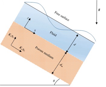
Sketch of the physical problem.

2 Theoretical framework
The problem analysed in the present study is same as that of DDB and is schematically represented in figure 1. We consider a film of fluid of mean height,
 $d$
with density,
 $\unicode[STIX]{x1D70C}$
kinematic viscosity,
 $\unicode[STIX]{x1D708}$
and surface tension,
 $\unicode[STIX]{x1D6FE}$
flowing over a porous layer of porosity,
 $\unicode[STIX]{x1D711}$
and thickness
 $d_{m}$
inclined at an angle
 $\unicode[STIX]{x1D703}$
to the horizontal. Let
 $t$
denote the time,
 $x$
be the streamwise coordinate and
 $z$
be the cross-stream coordinate (measured upwards from the porous–fluid interface). The permeability of the porous medium is expressed by the diagonal tensor
 $\unicode[STIX]{x1D646}=K_{x}\unicode[STIX]{x1D702}_{x}(z/d_{m})\boldsymbol{i}\boldsymbol{i}+K_{z}\unicode[STIX]{x1D702}_{z}(z/d_{m})\boldsymbol{k}\boldsymbol{k}$
where
 $\boldsymbol{i}$
and
 $\boldsymbol{k}$
are the unit vectors in
 $x$
and
 $z$
directions. The functions
 $\unicode[STIX]{x1D702}_{x}$
and
 $\unicode[STIX]{x1D702}_{z}$
describe the inhomogeneous variations in the permeability. We define the anisotropy parameter as
 $\unicode[STIX]{x1D709}=K_{x}/K_{z}$
. Let
 $z=h(x,t)$
locate the free surface of the fluid layer. The governing equations and boundary conditions are reproduced here from DDB for completeness. The flow in the fluid layer is described by the incompressible continuity and Navier–Stokes equations, given by
 $$\begin{eqnarray}\displaystyle & \displaystyle \frac{\unicode[STIX]{x2202}u}{\unicode[STIX]{x2202}x}+\frac{\unicode[STIX]{x2202}w}{\unicode[STIX]{x2202}z}=0 & \displaystyle\end{eqnarray}$$
 $$\begin{eqnarray}\displaystyle & \displaystyle \frac{\unicode[STIX]{x2202}u}{\unicode[STIX]{x2202}t}+u\frac{\unicode[STIX]{x2202}u}{\unicode[STIX]{x2202}x}+w\frac{\unicode[STIX]{x2202}u}{\unicode[STIX]{x2202}z}=-\frac{1}{\unicode[STIX]{x1D70C}}\frac{\unicode[STIX]{x2202}p}{\unicode[STIX]{x2202}x}+g\sin \unicode[STIX]{x1D703}+\unicode[STIX]{x1D708}\unicode[STIX]{x0394}u & \displaystyle\end{eqnarray}$$
 $$\begin{eqnarray}\displaystyle & \displaystyle \frac{\unicode[STIX]{x2202}w}{\unicode[STIX]{x2202}t}+u\frac{\unicode[STIX]{x2202}w}{\unicode[STIX]{x2202}x}+w\frac{\unicode[STIX]{x2202}w}{\unicode[STIX]{x2202}z}=-\frac{1}{\unicode[STIX]{x1D70C}}\frac{\unicode[STIX]{x2202}p}{\unicode[STIX]{x2202}z}-g\cos \unicode[STIX]{x1D703}+\unicode[STIX]{x1D708}\unicode[STIX]{x0394}w, & \displaystyle\end{eqnarray}$$
where
 $\boldsymbol{v}=(u,w)$
is the velocity,
 $p$
is the pressure,
 $g$
is the acceleration due to gravity and
 $\unicode[STIX]{x0394}$
denotes the two-dimensional Laplace operator. The continuity and generalized Darcy’s equations governing the flow through the porous medium are
 $$\begin{eqnarray}\displaystyle & \displaystyle \frac{\unicode[STIX]{x2202}u_{m}}{\unicode[STIX]{x2202}x}+\frac{\unicode[STIX]{x2202}w_{m}}{\unicode[STIX]{x2202}z}=0 & \displaystyle\end{eqnarray}$$
 $$\begin{eqnarray}\displaystyle & \displaystyle \frac{1}{\unicode[STIX]{x1D711}}\frac{\unicode[STIX]{x2202}u_{m}}{\unicode[STIX]{x2202}t}=-\frac{1}{\unicode[STIX]{x1D70C}}\frac{\unicode[STIX]{x2202}p_{m}}{\unicode[STIX]{x2202}x}-\frac{\unicode[STIX]{x1D708}}{K_{x}\unicode[STIX]{x1D702}_{x}(z/d_{m})}u_{m}+g\sin \unicode[STIX]{x1D703} & \displaystyle\end{eqnarray}$$
 $$\begin{eqnarray}\displaystyle & \displaystyle \frac{1}{\unicode[STIX]{x1D711}}\frac{\unicode[STIX]{x2202}w_{m}}{\unicode[STIX]{x2202}t}=-\frac{1}{\unicode[STIX]{x1D70C}}\frac{\unicode[STIX]{x2202}p_{m}}{\unicode[STIX]{x2202}z}-\frac{\unicode[STIX]{x1D708}}{K_{z}\unicode[STIX]{x1D702}_{z}(z/d_{m})}w_{m}-g\cos \unicode[STIX]{x1D703}, & \displaystyle\end{eqnarray}$$
where
 $\boldsymbol{v}_{m}=(u_{m},w_{m})$
is the Darcy velocity and
 $p_{m}$
is the intrinsic volume-averaged pressure. We acknowledge the existence of more detailed and complicated model such as the Darcy–Brinkman equation. Brinkman’s correction corresponds to the phenomenological inclusion of a viscous stress term in the Darcy’s law and its validity remains debated in the literature. However, a common agreement appears to be that Brinkman equation is valid for porous media with high porosity (Auriault Reference Auriault2009). A quantitative footing to this condition is given by Durlofsky & Brady (Reference Durlofsky and Brady1987), who showed using a Green’s function approach that the Brinkman equation is valid for
 $\unicode[STIX]{x1D711}>0.95$
. For the present study, we use
 $\unicode[STIX]{x1D711}=0.1$
, for which the validity of Brinkman’s correction is certainly questionable. Further uncertainties arise due to the lack of a clear definition of the ‘effective viscosity’ appearing in the Brinkman equation and the different forms of Brinkman equation and boundary conditions used in different papers (see Liu & Liu (Reference Liu and Liu2009) for a detailed discussion). Hence, in the parameter range of our interest, the classical Navier–Stokes/Darcy model best describes the flow through the porous medium, given that the accuracy/suitability of the extensions of Darcy’s law are not yet firmly settled in the literature.
The boundary conditions are:
 $$\begin{eqnarray}\displaystyle & \displaystyle w_{m}=0\quad \text{at}~z=-d_{m} & \displaystyle\end{eqnarray}$$
 $$\begin{eqnarray}\displaystyle & \displaystyle \left.\begin{array}{@{}c@{}}\displaystyle \frac{\unicode[STIX]{x2202}u}{\unicode[STIX]{x2202}z}=\frac{\unicode[STIX]{x1D6FC}}{\sqrt{K_{x}\unicode[STIX]{x1D702}_{x}(0)}}(u-u_{m})\\ \displaystyle p-2\unicode[STIX]{x1D707}\frac{\unicode[STIX]{x2202}w}{\unicode[STIX]{x2202}z}=p_{m}\\ w=w_{m}\end{array}\right\}\quad \text{at}~z=0 & \displaystyle\end{eqnarray}$$
 $$\begin{eqnarray}\displaystyle & \displaystyle \left.\begin{array}{@{}c@{}}\displaystyle w=\frac{\unicode[STIX]{x2202}h}{\unicode[STIX]{x2202}t}+u\frac{\unicode[STIX]{x2202}h}{\unicode[STIX]{x2202}x}\\ \displaystyle 2\unicode[STIX]{x1D707}\frac{\unicode[STIX]{x2202}w}{\unicode[STIX]{x2202}z}-p=\unicode[STIX]{x1D6FE}\frac{\unicode[STIX]{x2202}^{2}h/\unicode[STIX]{x2202}x^{2}}{(1+(\unicode[STIX]{x2202}h/\unicode[STIX]{x2202}x)^{2})^{3/2}}\\ \displaystyle \frac{\unicode[STIX]{x2202}w}{\unicode[STIX]{x2202}x}+\frac{\unicode[STIX]{x2202}u}{\unicode[STIX]{x2202}z}=0\end{array}\right\}\quad \text{at}~z=h(x,t), & \displaystyle\end{eqnarray}$$
with
 $\unicode[STIX]{x1D6FC}$
denoting the Beavers–Joseph coefficient. Equation (2.7) represents the no-penetration condition at the bottom surface of the porous layer. Equation (2.8) contains the Beavers–Joseph condition (Beavers & Joseph Reference Beavers and Joseph1967) prescribing the discontinuity in the tangential velocity, continuity of normal stress and continuity of the normal velocity at the interface between the fluid and porous layers. Finally, (2.9) describes the boundary conditions at the free surface of the liquid layer, namely, the kinematic condition, balance of normal stress and balance of shear stress.
Following Liu & Liu (Reference Liu and Liu2009), all the variables are normalized using
 $u_{0}$
,
 $d$
,
 $d/u_{0}$
,
 $\unicode[STIX]{x1D70C}u_{0}^{2}$
as the scales for velocity, length, time and pressure for the fluid layer and
 $\unicode[STIX]{x1D708}/d_{m}$
,
 $d_{m}$
,
 $d_{m}^{2}/\unicode[STIX]{x1D708}$
,
 $\unicode[STIX]{x1D70C}(\unicode[STIX]{x1D708}/d_{m})^{2}$
correspondingly for the porous layer. Here
 $u_{0}=d^{2}g\sin \unicode[STIX]{x1D703}/2\unicode[STIX]{x1D708}$
denotes the surface velocity of a fluid film falling on an impermeable substrate. Using an overbar to denote the base state, the steady parallel flow solution (
 $\bar{h}=1$
) is:
 $$\begin{eqnarray}\displaystyle & \displaystyle \bar{u}=-z^{2}+2z+2\unicode[STIX]{x1D6FD}+2\unicode[STIX]{x1D6FD}^{2}\unicode[STIX]{x1D6FC}^{2},\quad \bar{w}=0,\quad 0\leqslant z\leqslant 1 & \displaystyle\end{eqnarray}$$
 $$\begin{eqnarray}\displaystyle & \displaystyle \bar{u}_{m}=\frac{2\unicode[STIX]{x1D6FF}^{2}Re\unicode[STIX]{x1D702}_{x}(z_{m})}{\hat{d}^{3}},\quad \bar{w}_{m}=0,\quad -1\leqslant z_{m}\leqslant 0, & \displaystyle\end{eqnarray}$$
where
 $\hat{d}=d/d_{m}$
is the depth ratio,
 $\unicode[STIX]{x1D6FF}=\sqrt{K_{x}}/d_{m}$
is the Darcy number,
 $Re=u_{0}d/\unicode[STIX]{x1D708}$
is the Reynolds number and
 $\unicode[STIX]{x1D6FD}=\unicode[STIX]{x1D6FF}\sqrt{\unicode[STIX]{x1D702}_{x}(0)}/\unicode[STIX]{x1D6FC}\hat{d}$
.
The linear stability of this base state to two-dimensional perturbations is investigated. As can be seen from appendix A of the supplementary material available at https://doi.org/10.1017/jfm.2016.613, Squire’s transformation (Squire Reference Squire1933) does not appear to be applicable to the present problem. One cannot be certain at this point about the set of appropriate transformations, for a given set of parameters (
 $\unicode[STIX]{x1D709}$
,
 $\unicode[STIX]{x1D712}$
,
 $\unicode[STIX]{x1D702}_{x}$
,
 $\unicode[STIX]{x1D702}_{y}$
, etc.), that will reduce the three-dimensional system of perturbation equations to an equivalent two-dimensional system. Further, even in systems with an isotropic and homogeneous porous medium, the interfacial normal stress boundary condition is reported to preclude the application of Squires transformation (Camporeale et al.
Reference Camporeale, Mantelli and Manes2013). However, in terms of growth rate, two-dimensional disturbances were still found to be more dangerous, making a two-dimensional linear stability analysis worthwhile in such systems. Pressure is eliminated from the linearized perturbation equations and the velocity disturbances are expressed in terms of the streamfunctions
 $\unicode[STIX]{x1D713}$
and
 $\unicode[STIX]{x1D713}_{m}$
. Further, we introduce the normal modes
 $\unicode[STIX]{x1D713}=\unicode[STIX]{x1D6F7}(z)\text{e}^{\text{i}k(x-ct)}$
and
 $\unicode[STIX]{x1D713}_{m}=\unicode[STIX]{x1D6F7}_{m}(z_{m})\text{e}^{\text{i}k_{m}(x_{m}-c_{m}t_{m})}$
, where
 $k$
and
 $k_{m}$
denote the real wavenumber and
 $c$
and
 $c_{m}$
denote the complex wave speed, to obtain
 $$\begin{eqnarray}\displaystyle & \displaystyle \text{i}kc(D^{2}-k^{2})\unicode[STIX]{x1D6F7}=\text{i}k\bar{u}(D^{2}-k^{2})\unicode[STIX]{x1D6F7}-\text{i}k\unicode[STIX]{x1D6F7}D^{2}\bar{u}-\frac{1}{Re}(D^{2}-k^{2})^{2}\unicode[STIX]{x1D6F7} & \displaystyle\end{eqnarray}$$
 $$\begin{eqnarray}\displaystyle & \displaystyle -\frac{\text{i}k_{m}c_{m}}{\unicode[STIX]{x1D711}}(D_{m}^{2}-k_{m}^{2})\unicode[STIX]{x1D6F7}_{m}=-\frac{1}{\unicode[STIX]{x1D6FF}^{2}}\left(\frac{D_{m}^{2}\unicode[STIX]{x1D6F7}_{m}}{\unicode[STIX]{x1D702}_{x}}-\frac{\unicode[STIX]{x1D709}k_{m}^{2}}{\unicode[STIX]{x1D702}_{z}}\unicode[STIX]{x1D6F7}_{m}-\frac{{D_{m}\unicode[STIX]{x1D702}_{x}D}_{m}\unicode[STIX]{x1D6F7}_{m}}{\unicode[STIX]{x1D702}_{x}^{2}}\right) & \displaystyle\end{eqnarray}$$
subject to the following boundary conditions:
 $$\begin{eqnarray}\displaystyle & \displaystyle \unicode[STIX]{x1D6F7}_{m}(-1)=0\quad \text{at}~z_{m}=-1 & \displaystyle\end{eqnarray}$$
 $$\begin{eqnarray}\displaystyle & \displaystyle \hspace{-3.60004pt}\left.\begin{array}{@{}c@{}}\displaystyle D^{2}\unicode[STIX]{x1D6F7}(0)=\frac{1}{\unicode[STIX]{x1D6FD}}\left(D\unicode[STIX]{x1D6F7}(0)-\frac{\hat{d}}{Re}D_{m}\unicode[STIX]{x1D6F7}_{m}(0)\right)\\ \displaystyle \unicode[STIX]{x1D6F7}(0)=\frac{1}{Re}\unicode[STIX]{x1D6F7}_{m}(0)\\ \displaystyle \text{i}kcD\unicode[STIX]{x1D6F7}(0)-\frac{\hat{d}^{3}}{\unicode[STIX]{x1D711}\,Re^{2}}\text{i}k_{m}c_{m}D_{m}\unicode[STIX]{x1D6F7}_{m}(0)=-\frac{1}{Re}D^{3}\unicode[STIX]{x1D6F7}(0)+\frac{3}{Re}k^{2}D\unicode[STIX]{x1D6F7}(0)\\ \displaystyle +\,\bar{u}(0)\text{i}kD\unicode[STIX]{x1D6F7}(0)-\text{i}k\unicode[STIX]{x1D6F7}(0)D\bar{u}(0)-\frac{\hat{d}^{3}}{Re^{2}}\frac{D_{m}\unicode[STIX]{x1D6F7}_{m}(0)}{\unicode[STIX]{x1D6FF}^{2}\unicode[STIX]{x1D702}_{x}(0)}\end{array}\right\}\quad z=z_{m}=0\;\qquad \; & \displaystyle\end{eqnarray}$$
 $$\begin{eqnarray}\displaystyle & \displaystyle \left.\begin{array}{@{}c@{}}\displaystyle (D^{2}+k^{2})\unicode[STIX]{x1D6F7}(1)=-D^{2}\bar{u}(1)\left(\frac{\unicode[STIX]{x1D6F7}(1)}{c-\bar{u}(1)}\right)\\ \displaystyle \text{i}kcD\unicode[STIX]{x1D6F7}(1)=\text{i}k\bar{u}(1)D\unicode[STIX]{x1D6F7}(1)-\text{i}k\unicode[STIX]{x1D6F7}(1)D\bar{u}(1)-\frac{1}{Re}D^{3}\unicode[STIX]{x1D6F7}(1)\\ \displaystyle +\,\frac{3k^{2}}{Re}D\unicode[STIX]{x1D6F7}(1)+\left(\text{i}k^{3}S+\frac{2}{Re}\text{i}k\cot \unicode[STIX]{x1D703}\right)\left(\frac{\unicode[STIX]{x1D6F7}(1)}{c-\bar{u}(1)}\right)\end{array}\right\}\quad z=1, & \displaystyle\end{eqnarray}$$
where
 $D=(\text{d}/\text{d}z)$
,
 $D_{m}=(\text{d}/\text{d}z_{m})$
and
 $S=\unicode[STIX]{x1D6FE}/\unicode[STIX]{x1D70C}u_{0}^{2}\,\text{d}$
is the non-dimensional surface tension. Equivalently,
 $S=Re^{-5/3}((3/2)\sin \unicode[STIX]{x1D703})^{-1/3}\unicode[STIX]{x1D701}$
, where
 $\unicode[STIX]{x1D701}=(3\unicode[STIX]{x1D70C}\unicode[STIX]{x1D6FE}^{3}/g\unicode[STIX]{x1D707}^{4})^{1/3}$
is the surface tension number (Floryan et al.
Reference Floryan, Davis and Kelly1987). Note that
 $k=\hat{d}k_{m}$
and
 $c=(\hat{d}/Re)c_{m}$
.
An asymptotic solution to the above eigenvalue problem in the limit of long wavelength can be obtained by expanding the perturbation amplitudes,
 $\unicode[STIX]{x1D6F7}(z)$
,
 $\unicode[STIX]{x1D6F7}_{m}(z_{m})$
and
 $c$
in powers of
 $k$
(Yih Reference Yih1963; Pascal Reference Pascal1999) as
 $\unicode[STIX]{x1D6F7}=\unicode[STIX]{x1D6F7}^{(0)}(z)+\unicode[STIX]{x1D6F7}^{(1)}(z)k+O(k^{2})$
, with analogous expressions for the other variables. Substituting these expressions into (2.12)–(2.16) and collecting
 $O(1)$
terms leads to the eigenvalue problem given as follows.
 $$\begin{eqnarray}\displaystyle & \displaystyle D^{4}\unicode[STIX]{x1D6F7}^{(0)}=0 & \displaystyle\end{eqnarray}$$
 $$\begin{eqnarray}\displaystyle & \displaystyle \frac{D_{m}^{2}\unicode[STIX]{x1D6F7}_{m}^{(0)}}{D_{m}\unicode[STIX]{x1D6F7}_{m}^{(0)}}=\frac{D_{m}\unicode[STIX]{x1D702}_{x}}{\unicode[STIX]{x1D702}_{x}} & \displaystyle\end{eqnarray}$$
 $$\begin{eqnarray}\displaystyle & \displaystyle \unicode[STIX]{x1D6F7}_{m}^{(0)}(-1)=0 & \displaystyle\end{eqnarray}$$
 $$\begin{eqnarray}\displaystyle & \displaystyle D^{2}\unicode[STIX]{x1D6F7}^{(0)}(0)=\frac{1}{\unicode[STIX]{x1D6FD}}\left(D\unicode[STIX]{x1D6F7}^{(0)}(0)-\frac{\hat{d}}{Re}D_{m}\unicode[STIX]{x1D6F7}_{m}^{(0)}(0)\right) & \displaystyle\end{eqnarray}$$
 $$\begin{eqnarray}\displaystyle & \displaystyle \unicode[STIX]{x1D6F7}^{(0)}(0)=\frac{1}{Re}\unicode[STIX]{x1D6F7}_{m}^{(0)}(0) & \displaystyle\end{eqnarray}$$
 $$\begin{eqnarray}\displaystyle & \displaystyle \frac{1}{Re}D^{3}\unicode[STIX]{x1D6F7}^{(0)}(0)=-\frac{\hat{d}}{Re^{2}}\frac{D_{m}\unicode[STIX]{x1D6F7}_{m}^{(0)}(0)}{\unicode[STIX]{x1D6FD}^{2}\unicode[STIX]{x1D6FC}^{2}} & \displaystyle\end{eqnarray}$$
 $$\begin{eqnarray}\displaystyle & \displaystyle D^{2}\unicode[STIX]{x1D6F7}^{(0)}(1)=-D^{2}\bar{u}(1)\left(\frac{\unicode[STIX]{x1D6F7}^{(0)}(1)}{c^{(0)\prime }}\right) & \displaystyle\end{eqnarray}$$
 $$\begin{eqnarray}\displaystyle & \displaystyle D^{3}\unicode[STIX]{x1D6F7}^{(0)}(1)=0, & \displaystyle\end{eqnarray}$$
where
 $c^{(0)\prime }=c^{(0)}-\bar{u}(1)$
. The zeroth-order solution is obtained as:
 $$\begin{eqnarray}\displaystyle & \displaystyle \unicode[STIX]{x1D6F7}^{(0)}=\frac{z^{2}}{2}+\unicode[STIX]{x1D6FD}z & \displaystyle\end{eqnarray}$$
 $$\begin{eqnarray}\displaystyle & \displaystyle \unicode[STIX]{x1D6F7}_{m}^{(0)}=0 & \displaystyle\end{eqnarray}$$
 $$\begin{eqnarray}\displaystyle & \displaystyle c^{(0)}=2(1+2\unicode[STIX]{x1D6FD})+2\unicode[STIX]{x1D6FD}^{2}\unicode[STIX]{x1D6FC}^{2}. & \displaystyle\end{eqnarray}$$
One important observation is that at the zeroth-order level, there are no flow perturbations in the porous medium (this is true irrespective of the functional form of
 $\unicode[STIX]{x1D702}_{x}$
). In other words, at a zeroth-order approximation, it is sufficient to consider the double-layer system as a fluid layer flowing down an impermeable plane with a velocity-slip boundary condition, thus justifying the one-sided model employed by Pascal (Reference Pascal1999). This might also explain why Liu & Liu (Reference Liu and Liu2009), who compared the results of one-sided model with that from the two-sided model, found qualitative agreement at low to moderate values of permeability. As Yih (Reference Yih1963) has demonstrated, the surface waves on a fluid film on an inclined impermeable wall travel at twice the surface speed of the primary flow. Hence, the last two terms (containing
 $\unicode[STIX]{x1D6FD}$
) in (2.27) are corrections due to the presence of the porous substrate, which clearly increases the phase speed of the waves.
The succeeding eigenvalue problem (
 $O(k)$
equations) reads
 $$\begin{eqnarray}\displaystyle & \displaystyle D^{4}\unicode[STIX]{x1D6F7}^{(1)}=\text{i}\,Re[(\bar{u}-c^{(0)})D^{2}\unicode[STIX]{x1D6F7}^{(0)}-D^{2}\bar{u}\unicode[STIX]{x1D6F7}^{(0)}] & \displaystyle\end{eqnarray}$$
 $$\begin{eqnarray}\displaystyle & \displaystyle D_{m}^{2}\unicode[STIX]{x1D6F7}_{m}^{(1)}-\frac{D_{m}\unicode[STIX]{x1D702}_{x}}{\unicode[STIX]{x1D702}_{x}}D_{m}\unicode[STIX]{x1D6F7}_{m}^{(1)}=0 & \displaystyle\end{eqnarray}$$
 $$\begin{eqnarray}\displaystyle & \displaystyle \unicode[STIX]{x1D6F7}_{m}^{(1)}(-1)=0 & \displaystyle\end{eqnarray}$$
 $$\begin{eqnarray}\displaystyle & \displaystyle D^{2}\unicode[STIX]{x1D6F7}^{(1)}(0)=\frac{1}{\unicode[STIX]{x1D6FD}}\left(D\unicode[STIX]{x1D6F7}^{(1)}(0)-\frac{\hat{d}}{Re}D_{m}\unicode[STIX]{x1D6F7}_{m}^{(1)}(0)\right) & \displaystyle\end{eqnarray}$$
 $$\begin{eqnarray}\displaystyle & \displaystyle \unicode[STIX]{x1D6F7}^{(1)}(0)=\frac{1}{Re}\unicode[STIX]{x1D6F7}_{m}^{(1)}(0) & \displaystyle\end{eqnarray}$$
 $$\begin{eqnarray}\displaystyle & \displaystyle \text{i}c^{(0)\prime }D\unicode[STIX]{x1D6F7}^{(0)}(0)=-\frac{1}{Re}D^{3}\unicode[STIX]{x1D6F7}^{(1)}(0)-\frac{\hat{d}}{Re^{2}}\frac{D_{m}\unicode[STIX]{x1D6F7}_{m}^{(1)}(0)}{\unicode[STIX]{x1D6FD}^{2}\unicode[STIX]{x1D6FC}^{2}} & \displaystyle\end{eqnarray}$$
 $$\begin{eqnarray}\displaystyle & \displaystyle D^{2}\unicode[STIX]{x1D6F7}^{(1)}(1)=D^{2}\bar{u}(1)\left(\frac{\unicode[STIX]{x1D6F7}_{0}(1)}{c^{(0)^{\prime 2}}}c^{(1)}\right) & \displaystyle\end{eqnarray}$$
 $$\begin{eqnarray}\displaystyle & \displaystyle \text{i}c^{(0)\prime }D\unicode[STIX]{x1D6F7}^{(0)}(1)=-\frac{1}{Re}D^{3}\unicode[STIX]{x1D6F7}^{(1)}(1)-\frac{2\text{i}\cot \unicode[STIX]{x1D703}}{Re}\frac{\unicode[STIX]{x1D6F7}^{(0)}(1)}{c^{(0)\prime }}. & \displaystyle\end{eqnarray}$$
As can be seen from (2.29), the inhomogeneity function
 $\unicode[STIX]{x1D702}_{x}$
appears in the first-order problem. For obtaining exact solutions to the above and subsequent eigenvalue problems, we assume the following exponential variation for the permeability:
 $\unicode[STIX]{x1D702}_{x}=\text{e}^{A(1+z_{m})}$
. Note that in Green & Freehill (Reference Green and Freehill1969), the permeability is assumed to vary in a linear fashion with the depth of the porous layer. However, the exponential inhomogeneity function is an experimentally measured profile in a practical system (Chen Reference Chen1992); at any rate, for the purpose of this discussion, the actual functional form chosen is not critical and does not result in loss of generality. The solution to the above problem is
 $$\begin{eqnarray}\displaystyle & \displaystyle \unicode[STIX]{x1D6F7}^{(1)}=2\text{i}\,Re(1+\unicode[STIX]{x1D6FD})\left(\frac{z^{5}}{120}-\frac{z^{4}}{24}\right)+A_{1}\frac{z^{3}}{6}+A_{2}\frac{z^{2}}{2}+A_{3}z+A_{4} & \displaystyle\end{eqnarray}$$
 $$\begin{eqnarray}\displaystyle & \displaystyle \unicode[STIX]{x1D6F7}_{m}^{(1)}=\left\{\begin{array}{@{}ll@{}}B_{1}+B_{2}z_{m}, & \text{if}~A=0\\ B_{1}+B_{2}\text{e}^{Az_{m}}, & \text{otherwise}\end{array}\right. & \displaystyle\end{eqnarray}$$
 $$\begin{eqnarray}\displaystyle & \displaystyle c^{(1)}=\left\{\begin{array}{@{}ll@{}}\displaystyle \frac{4\text{i}\,Re(1+\unicode[STIX]{x1D6FD})(15\unicode[STIX]{x1D6FD}^{2}+10\unicode[STIX]{x1D6FD}+2)}{15} & \\ \quad \displaystyle -\,\frac{2\text{i}\cot \unicode[STIX]{x1D703}(1+3\unicode[STIX]{x1D6FD})}{3}-2\text{i}\unicode[STIX]{x1D6FC}^{2}\unicode[STIX]{x1D6FD}^{2}\cot \unicode[STIX]{x1D703}\left(1+\frac{1}{\hat{d}}\right), & \text{if}~A=0\\ \displaystyle \frac{4\text{i}\,Re(1+\unicode[STIX]{x1D6FD})(15\unicode[STIX]{x1D6FD}^{2}+10\unicode[STIX]{x1D6FD}+2)}{15} & \\ \quad \displaystyle -\,\frac{2\text{i}\cot \unicode[STIX]{x1D703}(1+3\unicode[STIX]{x1D6FD})}{3}-2\text{i}\unicode[STIX]{x1D6FC}^{2}\unicode[STIX]{x1D6FD}^{2}\cot \unicode[STIX]{x1D703}\left(1-\frac{\text{e}^{-A}-1}{A\hat{d}}\right), & \text{otherwise}.\end{array}\right.\qquad & \displaystyle\end{eqnarray}$$
The constants
 $A_{1}$
to
 $A_{4}$
,
 $B_{1}$
and
 $B_{2}$
are compiled in appendix B in the supplementary material. From the expression for
 $c^{(1)}$
we obtain the following first-order approximation for the critical Reynolds number of long-wave disturbances
 $Re_{0}$
:
 $$\begin{eqnarray}Re_{0}=\left\{\begin{array}{@{}ll@{}}\displaystyle \frac{15}{4(1+\unicode[STIX]{x1D6FD})(15\unicode[STIX]{x1D6FD}^{2}+10\unicode[STIX]{x1D6FD}+2)} & \\ \quad \displaystyle \times \left[\frac{2\cot \unicode[STIX]{x1D703}(1+3\unicode[STIX]{x1D6FD})}{3}+2\unicode[STIX]{x1D6FC}^{2}\unicode[STIX]{x1D6FD}^{2}\cot \unicode[STIX]{x1D703}\left(1+\frac{1}{\hat{d}}\right)\right], & \text{if}~A=0\\ \displaystyle \frac{15}{4(1+\unicode[STIX]{x1D6FD})(15\unicode[STIX]{x1D6FD}^{2}+10\unicode[STIX]{x1D6FD}+2)} & \\ \quad \displaystyle \times \left[\frac{2\cot \unicode[STIX]{x1D703}(1+3\unicode[STIX]{x1D6FD})}{3}+2\unicode[STIX]{x1D6FC}^{2}\unicode[STIX]{x1D6FD}^{2}\cot \unicode[STIX]{x1D703}\left(1-\frac{\text{e}^{-A}-1}{A\hat{d}}\right)\right], & \text{otherwise}.\end{array}\right.\quad\end{eqnarray}$$
We find that by substituting
 $\unicode[STIX]{x1D6FD}=0$
we will recover the expression for the critical Reynolds number in the case of impermeable wall as reported by Yih (Reference Yih1963), namely,
 $Re_{c}=(5/4)\cot \unicode[STIX]{x1D703}$
. The coefficient is different in Yih’s expression because we have used surface velocity of the equilibrium flow as the velocity scale.
The system of equations and solutions at
 $O(k^{2})$
and
 $O(k^{3})$
is provided in appendices C–F of the supplementary material. Note that
 $c^{(0)}$
and
 $c^{(2)}$
are real and
 $c^{(1)}$
and
 $c^{(3)}$
are imaginary. Hence the growth rate of a particular disturbance mode is
 $\unicode[STIX]{x1D70E}=k^{2}[\text{Im}(c^{(1)})+k^{2}\,\text{Im}(c^{(3)})]$
, while its phase speed is
 $\unicode[STIX]{x1D714}=c^{(0)}+k^{2}c^{(2)}$
. Setting
 $\unicode[STIX]{x1D70E}=0$
one can get the neutral stability curve in
 $Re-k$
plane for a given set of the other parameters involved. It is obvious that the entire
 $Re$
axis forms a part of the neutral stability curve. The other part of the curve is given by
 $k_{cri}=[-\text{Im}(c^{(1)})/\text{Im}(c^{(3)})]^{1/2}$
and it bifurcates from the
 $Re$
axis at the point
 $Re_{0}$
.
3 Results
3.1 Homogeneous and isotopic porous substrate
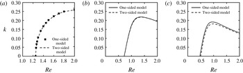
For the purpose of verification of our theoretical analysis, we compare the neutral stability curves obtained from the one-sided model (Pascal Reference Pascal1999) and our two-sided model for
 $\unicode[STIX]{x1D6FD}=0$
(which simulates the flow of fluid over an impermeable substrate) in figure 2(a) and good agreement is obtained. When
 $\unicode[STIX]{x1D6FD}$
is increased (cf. figure 2
b,c), however, the one-sided model tends to underestimate the critical stability conditions and the disagreement becomes large at higher values of
 $\unicode[STIX]{x1D6FD}$
. In this discussion, the porous medium is considered to be homogeneous (
 $A=0$
) and isotropic (
 $\unicode[STIX]{x1D709}=1$
). The disagreement between the two-sided and one-sided model was also found numerically by Liu & Liu (Reference Liu and Liu2009); however, it may be worth mentioning that since it underestimates the critical conditions, the one-sided model gives a conservative prediction, thus justifying its use. However, in order to model the heterogeneity and anisotropy of the porous medium, it is indispensable to implement a two-sided approach, as detailed in the previous section.
Comparison of marginal curves obtained from one-sided model and two-sided model for various values of
 $\unicode[STIX]{x1D6FD}$
. (a)
 $\unicode[STIX]{x1D6FD}=0$
, (b)
 $\unicode[STIX]{x1D6FD}=0.2$
, (c)
 $\unicode[STIX]{x1D6FD}=0.4$
. Angle of inclination,
 $\unicode[STIX]{x1D703}=\unicode[STIX]{x03C0}/4$
.

Now let us examine the effect of surface tension on the stability of the system. The correction due to the surface tension number,
 $\unicode[STIX]{x1D701}$
enters only at third order in
 $k$
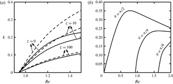
. Hence surface tension does not have any role to play in the stability of infinitely long perturbations, as shown in figure 3(a), where the intercept of the marginal stability curves with the
 $Re$
axis appears to be insensitive to
 $\unicode[STIX]{x1D701}$
. However, as expected, a higher
 $\unicode[STIX]{x1D701}$
indeed stabilizes moderately long disturbances. As a result the unstable region in the
 $Re-k$
plane shrinks as
 $\unicode[STIX]{x1D701}$
increases.
Neutral stability curves. (a) Effect of surface tension number,
 $\unicode[STIX]{x1D701}$
, at
 $\unicode[STIX]{x1D703}=\unicode[STIX]{x03C0}/4$
. Solid curves represent theoretical results and dashed curves represent numerical results. (b) Effect of angle of inclination,
 $\unicode[STIX]{x1D703}$
at
 $\unicode[STIX]{x1D701}=0$
. The other parameters are
 $\hat{d}=0.1$
,
 $\unicode[STIX]{x1D6FF}=0.001$
and
 $\unicode[STIX]{x1D6FC}=0.1$
.

The corresponding neutral curves obtained from the numerical solution of the two-sided model described in DDB are also plotted in figure 3(a) and confirms this trend. As expected at larger
 $k$
, the disagreement between the theoretical and numerical curves is greater because the theoretical results are based on small-
 $k$
approximation. However, in the limit of
 $k\rightarrow 0$
, the theoretical predictions asymptotically approach the numerical results and this serves as another measure of verification of the theoretical model. For the rest of the paper, to offer a conservative estimate of the stability limit, we choose
 $\unicode[STIX]{x1D701}=0$
.
Also one may notice that that the inhomogeneity function for the cross-stream component of permeability,
 $\unicode[STIX]{x1D702}_{z}$
does not appear in the eigenvalue problems up to
 $O(k)$
; nor do porosity of the porous layer (
 $\unicode[STIX]{x1D711}$
) and the anisotropy parameter (
 $\unicode[STIX]{x1D709}$
). The reason is quite evident from the linearized perturbation equations (2.12)–(2.16), where the terms involving these parameters contain (explicitly or implicitly) powers of
 $k$
higher than 1. Consequently, these parameters play minimal role in the stability of the system. Furthermore, the effect of angle of inclination is quite evident from (2.39). For
 $\unicode[STIX]{x1D703}=\unicode[STIX]{x03C0}/2$
,
 $Re_{0}=0$
, i.e. a vertical porous–fluid double layer is unconditionally unstable. Keeping all other parameters fixed, as
 $\unicode[STIX]{x1D703}$
is varied from
 $\unicode[STIX]{x03C0}/4$
to 0,
 $\cot \unicode[STIX]{x1D703}$
increases; so does
 $Re_{0}$
. In other words, gravity has a monotonic destabilizing effect, which is further illustrated in figure 3(b), where the neutral stability curves for different angles of inclination are plotted. Hence for demonstrating the effect of key parameters in the following results, we fix
 $\unicode[STIX]{x1D703}=\unicode[STIX]{x03C0}/4$
(same as in Sadiq & Usha Reference Sadiq and Usha2008). In the range of parameters considered here we find that porosity,
 $\unicode[STIX]{x1D711}$
has very little effect on the stability characteristics We set
 $\unicode[STIX]{x1D711}=0.1$
for the subsequent analyses.
Before discussing the results any further, it is useful to note that in Pascal (Reference Pascal1999), the influence of the parameters
 $\unicode[STIX]{x1D6FF}$
,
 $\hat{d}$
and
 $\unicode[STIX]{x1D6FC}$
could be described in terms of a single parameter
 $\unicode[STIX]{x1D6FD}^{\prime }$
defined as
 $\unicode[STIX]{x1D6FD}^{\prime }=\unicode[STIX]{x1D6FF}/\unicode[STIX]{x1D6FC}\hat{d}$
. However, on inspection of the current eigenvalue problems, it follows that
 $\unicode[STIX]{x1D6FD}^{\prime }$
alone does not capture the collective effect of these parameters and hence is irrelevant for the present study. The reason is twofold: first, we follow the two-sided approach to take into account the non-negligible flow in the porous layer; second, Pascal (Reference Pascal1999) retains terms only up to
 $O(\unicode[STIX]{x1D6FD}^{\prime 2})$
, whereas no terms are truncated in the current solution. Hence in this paper, we shall investigate the effect of each of these parameters individually. In the following sections, we first focus on the stability of the system with an inhomogeneous and isotropic porous substrate by setting
 $\unicode[STIX]{x1D702}_{x}=\unicode[STIX]{x1D702}_{z}=\text{e}^{A(1+z_{m})}$
and
 $\unicode[STIX]{x1D709}=1$
. Subsequently we shall consider the case of homogeneous but anisotropic porous substrate with
 $\unicode[STIX]{x1D702}_{x}=\unicode[STIX]{x1D702}_{z}=1$
.
3.2 Heterogeneous porous substrate
In order to illustrate the general trends and to reduce the parameter space, we first look at the solutions up to first order in
 $k$
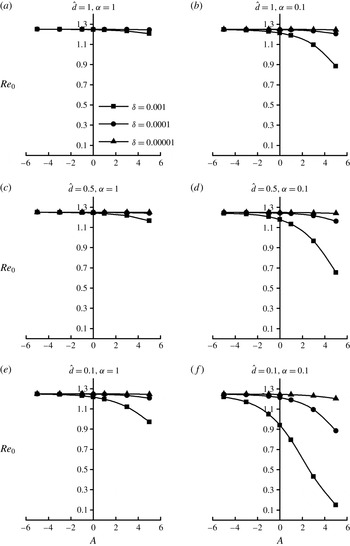
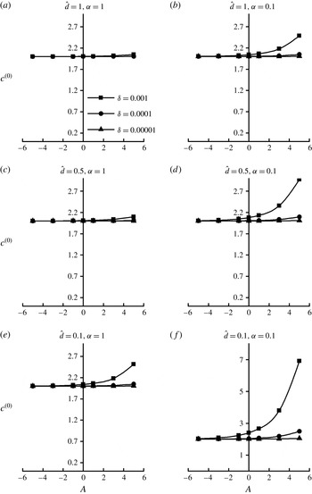
. Figure 4 presents the variation of
 $Re_{0}$
as a function of
 $A$
,
 $\unicode[STIX]{x1D6FF}$
,
 $\hat{d}$
and
 $\unicode[STIX]{x1D6FC}$
. As evident from each subfigure, systems with higher Darcy number (
 $\unicode[STIX]{x1D6FF}$
) become linearly unstable at a lower
 $Re_{0}$
. Also, for a given Darcy number (which is defined based on the permeability value at the bottom of the porous layer), as
 $A$
is increased, the system tends to become more unstable. This is because a higher value of
 $A$
implies that the porous layer is relatively more permeable near the interface between the porous/fluid layers, thus allowing the flow disturbances to easily penetrate into the porous layer. In other words, higher
 $A$
implies more fluid in the porous layer. This also explains why the destabilizing effect of permeability is more conspicuous at higher values of
 $A$
.
 $Re_{0}$
as a function of
 $A$
for different values of Darcy number,
 $\unicode[STIX]{x1D6FF}$
(as given in the legend). Legends are the same in all the panels.

The comparison of the different graphs in figure 4 shows that thinner fluid layers (relative to the porous layer) are more susceptible to instabilities. A lower Beavers–Joseph coefficient also reduces
 $Re_{0}$
. The former observation was also made in DDB, while the stabilizing effect of increase in Beavers–Joseph coefficient was also reported in the numerical work of Liu & Liu (Reference Liu and Liu2009). The reason for this is as follows. A higher
 $\unicode[STIX]{x1D6FC}$
translates to a higher velocity gradient (or stress) at the interface between the two layers, leading to larger frictional resistance and subsequent stabilization of the flow.
Another noteworthy point is that for increasing negative values of
 $A$
,
 $Re_{0}$
is seen to approach the critical Reynolds number for the impermeable wall case,
 $Re_{c}=(5/4)\cot \unicode[STIX]{x1D703}=1.25$
(for
 $\unicode[STIX]{x1D703}=\unicode[STIX]{x03C0}/4$
). This implies that for a sharp decrease of permeability in the vertical direction, the two layers decouple from each other and the system essentially reduces to a fluid layer on an impenetrable incline. The reason becomes obvious if one considers the eigenfunction in a porous medium at first order, as given in (2.37) (note that the zeroth-order eigenfunction corresponding to the porous layer is zero). It is clear that the disturbance streamfunction of the porous layer indeed follows a similar exponential behaviour as the permeability. Hence at very high negative values of
 $A$
, the flow disturbances in the porous layer near the porous–fluid interface will be almost absent. Subsequently, the flow perturbations that occur near the bottom of the porous layer become inconsequential to the stability of the surface waves as the connection between the two layers is broken at the interface. Thus the effect of the underlying porous layer and the changes in its permeability (whether through
 $A$
or
 $\unicode[STIX]{x1D6FF}$
) on the system stability is rendered insignificant, explaining the merging of the curves corresponding to different
 $\unicode[STIX]{x1D6FF}$
at very high negative values of
 $A$
, but the critical value of
 $A$
at which this merging happens becomes smaller and smaller as
 $\hat{d}$
and/or
 $\unicode[STIX]{x1D6FC}$
is decreased. In these cases, the effect of the presence of the porous layer on the overall system will be stronger (Liu & Liu Reference Liu and Liu2009). For example, in figure 4(f) (
 $\hat{d}=0.1$
and
 $\unicode[STIX]{x1D6FC}=0.1$
) even at
 $A=-3$
(vertically decreasing permeability), the effect of change in Darcy number is not negligible, whereas in Fig. 4a (
 $\hat{d}=1$
and
 $\unicode[STIX]{x1D6FC}=1$
) the change in Darcy number seems to be almost insignificant even for positive values of
 $A$
(vertically increasing permeability).
Figure 5 shows the effect of inhomogeneity in permeability on the zeroth-order phase speed of the free-surface waves for the same cases considered in figure 4. As expected from (2.27), a higher value of
 $A$
increases the wave speed (note that the parameter
 $\unicode[STIX]{x1D6FD}$
is a function of
 $A$
). Additionally, wave speed exhibits same qualitative trends in terms of the other system parameters such as
 $Re_{0}$
, as was explained above. For instance, the non-dimensional phase speed is observed to approach the value of 2 (corresponding to the speed of surface waves on a fluid film flowing down an impermeable inclined wall), as
 $A$
decreases. Irrespective of the value of permeability at the bottom of the porous layer (quantified by
 $\unicode[STIX]{x1D6FF}$
), if the permeability at the interface is low enough to decouple the two layers, the fluid flow mimics the condition where the substrate is impenetrable. Further, the effects of permeability and its inhomogeneity is more pronounced in cases where
 $\hat{d}$
and/or
 $\unicode[STIX]{x1D6FC}$
is smaller.
Non-dimensional phase speed of the surface waves as a function of
 $A$
for different values of Darcy number,
 $\unicode[STIX]{x1D6FF}$
(as given in the legend). Legends are the same in all the plots. Note that the scale of the vertical axis is not consistent across the graphs.

Phase speed as a function of wavenumber for various values of
 $A$
and
 $\unicode[STIX]{x1D6FF}=0.001$
at
 $Re=1$
. Legends are the same in all the panels.

Neutral stability curves for various values of
 $A$
and
 $\unicode[STIX]{x1D6FF}=0.001$
. Legends are the same in all the panels.

Since a higher Darcy number is found to be the most unstable case, let us now present the results concerning the higher-order solutions only for
 $\unicode[STIX]{x1D6FF}=0.001$
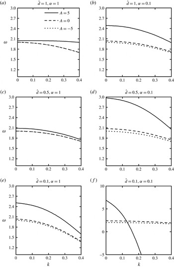
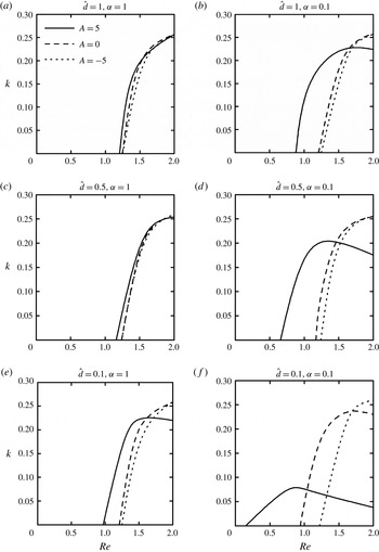
. In the current framework of linear stability analysis employing Darcy’s law, we do not attempt to consider higher values of Darcy number, because as Tilton & Cortelezzi (Reference Tilton and Cortelezzi2008) points out, at very high values of permeability, the convective terms in the equation describing the flow in the porous medium will be non-negligible. In figures 6 and 7 the variation of phase speed with wavenumber and the neutral stability curves are plotted respectively for
 $A=-5$
, 0 and 5. From figure 6, it is evident that for a given set of conditions, longer waves are observed to travel faster, a finding which is consistent with the dispersion relation of gravity waves. The general trend of phase speed increasing with
 $A$
, which was already explained using the zeroth-order results, is observed for a wide range of long-wave perturbations. Most of the other observations discussed in the previous paragraphs in the context of the infinitesimally long waves are extendable to higher wavenumbers as well. The effect of heterogeneity in permeability is more conspicuous at lower
 $\hat{d}$
and/or
 $\unicode[STIX]{x1D6FC}$
. In the limiting case of permeability decreasing vertically with high enough spatial rate, the fluid/porous double-layer system reduces to a fluid film over an impervious inclined plane.
For example, in figure 6(a), the curves for
 $A=-5$
and 0 are indistinguishable from each other. However in cases where the effect of porous layer is very dominant, such as a low
 $\hat{d}$
and/or
 $\unicode[STIX]{x1D6FC}$
, the higher-order solutions reveal a complicated behaviour. It is interesting to note from the neutral stability curves (figure 7) that although increasing
 $A$
has a monotonic destabilizing effect on infinitesimally long waves, it stabilizes the moderately long waves. Consequently, the boundary of the unstable region is pushed towards the low-wavenumber region with increasing
 $A$
.
(a) Variation of disturbance growth rate with wavenumber for subcritical and supercritical Reynolds numbers. (b) Comparison of critical wavenumber (
 $k_{cri}$
) and wavenumber corresponding to maximal growth rate (
 $k_{max}$
).
 $A=5$
,
 $\hat{d}=1$
and
 $\unicode[STIX]{x1D6FC}=1$
.

For
 $A=5$
,
 $\hat{d}=1$
and
 $\unicode[STIX]{x1D6FC}=1$
, the growth rate of the perturbations,
 $\unicode[STIX]{x1D70E}$
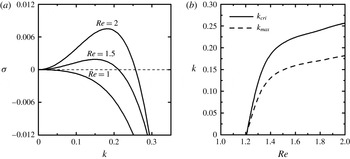
as a function of their wavenumbers is plotted in figure 8(a) at a sub-critical Reynolds number of 1 and super-critical Reynolds numbers of 1.5 and 2. As was apparent from the neutral stability curves, above the critical condition, a range of wavenumbers starts becoming unstable (manifested by a positive
 $\unicode[STIX]{x1D70E}$
).
However, the most dangerous perturbation will exhibit a wavenumber,
 $k_{max}$
(corresponding to the maximum growth rate) that can be obtained from
 $\unicode[STIX]{x2202}\unicode[STIX]{x1D70E}/\unicode[STIX]{x2202}k=0$
. This yields
 $k_{max}=k_{cri}/\sqrt{2}$
. In figure 8(b), we plot
 $k_{cri}$
and
 $k_{max}$
as a function of Reynolds number for the same parameters used in figure 8(a). We note that the
 $k_{cri}$
curve is the neutral stability curve. In an experiment where nonlinear effects are absent, for a given Reynolds number, the perturbation with wavenumber
 $k_{max}$
is most likely to be detected.
3.3 Anisotropic porous substrate
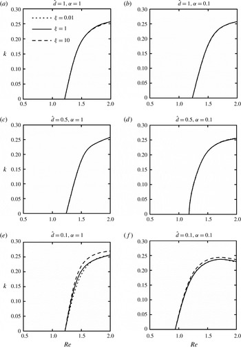
Here we consider a homogeneous but anisotropic porous substrate. The marginal stability curves for
 $\unicode[STIX]{x1D709}=0.01$
, 1 and 10 at different depth ratios and Beavers–Joseph coefficients are presented in figure 9. From the asymptotic analysis, it is seen that the effect of anisotropic parameter,
 $\unicode[STIX]{x1D709}$
, arises only in the third order of the perturbation solution. Hence it is expected to have a lesser effect than the heterogeneity in the permeability of the porous layer. This can be noticed through a comparison of figure 9 with figure 7. As expected from (2.39), at the intercept of the marginal stability curves with the
 $Re$
axis,
 $Re_{0}$
is independent of the anisotropic parameter. The insensitivity of the critical Reynolds number of the surface instability mode to the anisotropy parameter was also evident in the numerical results of DDB – the reason for which is now clear,
 $\unicode[STIX]{x1D709}$
has only higher-order contributions to the flow stability.
Neutral stability curves for various values of
 $\unicode[STIX]{x1D709}$
and
 $\unicode[STIX]{x1D6FF}=0.001$
. Legends are the same in all the panels.

However, the unstable region is seen to expand slightly with an increase in
 $\unicode[STIX]{x1D709}$
(figure 9). Note that for the shear mode of instability, it is observed that an increase in
 $\unicode[STIX]{x1D709}$
has a stabilizing effect (DDB); but for the surface mode of instability, it appears to have the opposite effect in the moderate-wavenumber region. A possible explanation for this observation is as follows. An increase in
 $\unicode[STIX]{x1D709}$
can be looked upon as either a relative increase of permeability in the
 $x$
direction,
 $K_{x}$
, or a relative decrease of permeability in the
 $z$
direction,
 $K_{z}$
. In the case of the shear mode, as already explained by DDB, a relative decrease in
 $K_{z}$
makes it more difficult for the flow perturbations to penetrate into the porous layer, thereby stabilizing the shear waves. Under favourable conditions, the results of the eigenvalue analysis have shown that the onset of shear mode instability can occur both in the fluid and porous layers. On the other hand, the surface mode is a pure fluid mode (onset of instability occurs only in the fluid layer) and hence the relative change of permeability in the wall normal direction plays no significant role. However, the relative increase of permeability in the mean flow direction offers less resistance to the flow disturbances at the fluid–porous layer interface and thus destabilizes the mode slightly.
4 Conclusions
In summary, we examined the stability of a fluid film on an inclined porous layer, whose permeability is allowed to be anisotropic and inhomogeneous under isothermal conditions. In order to capture the effects of the porous medium on the system, the coupled fluid–porous model was solved analytically based on long-wave asymptotic expansions. Nevertheless, the flow perturbations in the porous layer is found to be absent at the zeroth-order level. The major factors that are found to have first-order effects on the onset of instability are the angle of inclination (
 $\unicode[STIX]{x1D703}$
), the streamwise component of permeability (quantified by Darcy number,
 $\unicode[STIX]{x1D6FF}$
) and its inhomogeneous character (expressed in terms of the inhomogeneity factor,
 $A$
), the depth ratio (
 $\hat{d}$
) and the Beavers–Joseph coefficient (
 $\unicode[STIX]{x1D6FC}$
). For example, for a system with a vertically increasing permeability (positive
 $A$
), lower depth ratio and/or lower Beavers–Joseph coefficient, the destabilizing effect of the presence of porous layer is more pronounced and hence becomes less stable. In the range of parameters studied, for the same relative changes in Beavers–Joseph coefficient and depth ratio, the critical Reynolds number for the long-wave instability is more sensitive to the change in Beavers–Joseph coefficient.
If the vertical rate of decrease of permeability exceeds a level determined by the values of the other parameters, the stability behaviour of the free-surface waves of infinitesimally long wavelength will no longer be affected by the presence of the porous layer and the system reduces to the more stable configuration of a thin liquid film falling down on an inclined impermeable wall. A vertically increasing permeability, on the other hand, is found to destabilize the infinitesimally long waves and stabilize the moderately long waves. A vertically increasing permeability is also shown to increase the phase speed of the long-wave disturbances at the liquid–gas interface. These effects are more prominent in cases where the presence of porous layer is dominant, e.g. low relative fluid layer depth, low Beavers–Joseph coefficient and/or high permeability.
The effect of porosity and surface tension appears only at second and third orders of the perturbation problem respectively and hence these parameters have little effect on infinitely long-wave disturbances. As reported by DDB, the inhomogeneous variation in the permeability has a more pronounced effect compared to the anisotropic variation. Through the asymptotic analysis carried out in the present work, the reason for this becomes abundantly clear. The anisotropy parameter only has third-order effects on the onset of the instability, whereas the inhomogeneity function appears at the zeroth-order problem itself. Hence the anisotropy parameter has hardly any influence on the infinitesimally long waves, but a relative increase in permeability in the streamwise direction compared to that in the cross-stream direction is shown to stabilize the moderately long waves. Consequently it follows that, for a given set of system parameters, by controlling the anisotropic and/or inhomogeneous variation in the permeability, the onset of interfacial instability can be promoted or impeded. This is a valuable observation that can contribute to applications where the control of the hydrodynamic instability is desirable, e.g. in heat exchangers, an enhancement of the instability would result in an increased interfacial area available for heat transport. The permeability of the porous layer can be strategically modulated (instead of changing it throughout the depth of the porous layer) to achieve the desired level of instability.
Acknowledgement
The authors are grateful to the anonymous referees for their valuable comments.
Supplementary material
Supplementary material is available at https://doi.org/10.1017/jfm.2016.613.