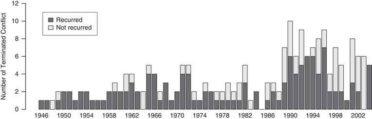


The end of fighting cannot be equated with eternal peace. As illustrated in Figure 1, 63 percent of civil conflicts recurFootnote 1 and we know that a history of armed conflict makes recurrence even more likely (Walter Reference Walter2004). In the long run we can therefore observe multiple peace and armed conflict spells with varying durations in one and the same conflict (Kreutz Reference Kreutz2010). Just reviewing this simple empirical insight already raises the main question of this paper: What is the extent to which pre-conflict, conflict, and post-conflict durations depend on each other? Only recently, scholars are taking seriously the notion that peace and armed conflict durations are interdependent processes that require detailed theoretical and empirical attention (Reed Reference Reed2000; Wagner Reference Wagner2000; Filson and Werner Reference Filson and Werner2002; Wucherpfennig Reference Wucherpfennig2011). However, most empirical efforts to identify the causes of pre-conflict, conflict, and post-conflict durations typically investigate the phases of peace (i.e., survival of peace until conflict breaks out) and the phases of conflict (survival of conflict until peace resumes) as two unrelated, isolated processes (Collier, Hoeffler and Soderbom Reference Collier, Hoeffler and Soderbom2004; Walter Reference Walter2004; Hegre and Sambanis Reference Hegre and Sambanis2006; Quinn, Mason and Gurses Reference Quinn, Mason and Gurses2007; Balch-Lindsay, Enterline and Joyce Reference Beck, Katz and Tucker2008). In this paper, we argue that peace (pre- and post-conflict) and conflict durations are interdependent, but highlight that there might be conditions under which actors decide never to fight. For example, if actors expect very high costs of conflict, we should never observe a conflict period. Thus, we have to differentiate between (1) peace spells that are actually at risk of conflict and (2) peace durations that are virtually immune to conflict. We demonstrate that a substantial increase in prediction performance of conflict and post-conflict duration can be achieved by taking into account all aspects of the theoretically implied data-generating process.
Conflict recurrence over time, 1946–2004
Note: this figure shows the frequency of conflict recurrence based on the Uppsala Conflict Data Program data set. The height of the bars shows the number of civil conflicts terminated in a given year. The light gray bars show the number of terminated conflicts that have not recurred by the end of 2004, and the black bars show the number of terminated conflicts that have recurred by the end of 2004.

Our main contribution is to introduce a split-population (SP) interdependent duration estimator that captures the theoretically implied unobserved interdependence between the durations of pre-conflict peace, conflict, and post-conflict peace. A major goal of this paper is to expand on the current literature that predominantly treats peace and conflict processes as independent (Walter Reference Walter2009; Blattman and Miguel Reference Blattman and Miguel2010). Theoretical and empirical research on the determinants of conflict onset (pre-conflict duration) is well developed and probably represents the largest share of existing civil conflict literature (Fearon and Laitin Reference Fearon and Laitin2003; Collier, Hoeffler and Soderbom Reference Collier, Hoeffler and Soderbom2004; Hegre and Sambanis Reference Hegre and Sambanis2006). Although not to the same extent, our knowledge about conflict durations has greatly expanded in recent years and many factors have been identified that impact on the decisions to continue or end fighting (Balch-Lindsay and Enterline Reference Balch-Lindsay and Enterline2000; Fearon Reference Fearon2004; Cunningham Reference Cunningham2006). Finally, scholars have been well aware of the fact that it is important to understand the conditions under which conflicts recur and have explored post-conflict durations both theoretically and empirically (Hartzell and Hoddie Reference Hartzell and Hoddie2003; Fortna Reference Fortna2003; Walter Reference Walter2004; Werner and Yuen Reference Werner and Yuen2005; Chiba Reference Chiba2015).
Despite the important contributions analyzing conflict and peace durations independently, less research is considering conflict and peace durations as interdependent processes (Hays and Kachi Reference Hays and Kachi2011). Although some significant contributions have been made that point to the importance of endogenous processes in conflicts (Reed Reference Reed2000; Boehmke, Morey and Shannon Reference Boehmke, Morey and Shannon2006; Wucherpfennig Reference Wucherpfennig2011), the more general conflict literature has not fully embraced the consequences of these duration interdependencies. In addition, when scholars address endogenous conflict processes they focus on the “dyadic duration” interdependence. This means these studies either focus on the relationship between (a) pre-conflict peace and fighting or (b) fighting and post-conflict peace. Naturally, this gives rise to a sample selection issue. For example, if we take into account the interdependence between conflict duration and post-conflict peace duration, we only allow cases into our sample that have actually experienced conflict. There are many approaches that might take care of this selection effect or split sample. However, the problem with existing approaches is that they take care of selection-duration and split-duration processes, but do not allow us to model what we think is the underlying data-generating process: a split-population duration-duration-duration process.
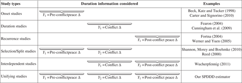
Consider Table 1 illustrating our three-duration concepts (pre-conflict peace, conflict, and post-conflict peace). Studies that explain conflict onset usually focus on pre-conflict peace and, depending on the research design, may also treat recurrence periods as pre-conflict spells. That implies that any information on conflict duration is not considered. In addition, peace spells are treated as independent and identically distributed and therefore possible interdependence is not considered. This is especially problematic when studies include conflicts with recurrent fighting and peace patterns, because they are likely to be linked to one another. Similarly, studies that focus on conflict duration treat fighting spells as independent from peace spells. A few studies have looked at “dyadic duration” dependence, that is allowing for interdependence between either pre-conflict peace spells and conflict spells or conflict spells and post-conflict peace spells (Reed Reference Reed2000; Boehmke, Morey and Shannon Reference Boehmke, Morey and Shannon2006; Wucherpfennig Reference Wucherpfennig2011). However, each of these empirical approaches does not utilize all observed information. In this paper, we seek to address this limitiation.
Existing Duration Studies and Limitations in the Amount of Information Considered

Note: SPDDD, split-population duration-duration-duration.
Although the empirical assessment of armed conflicts has sidelined interdependent durations, the theoretical literature is well aware of this relationship. Recent formal work on organized violence has conceptualized the onset, continuation, termination, and recurrence of wars as an interrelated bargaining process (Wagner Reference Wagner2000; Filson and Werner Reference Filson and Werner2002; Powell Reference Powell2004; Leventoglu and Slantchev Reference Leventoglu and Slantchev2007); however, even though the scholarly community has made considerable progress in developing detailed data sets on various aspects of conflict dynamics over the past decades,Footnote 2 the analytical and predictive tools available to the empirical researchers have not yet caught up with the developments in current conflict theories.
We propose a new empirical approach to study phases of peace and conflict in a single, unified survival analysis framework. Survival analysis (also called event history analysis, hazard analysis, or duration analysis) has become a widely used statistical approach to analyze political events (Box-Steffensmeier and Zorn Reference Box-Steffensmeier and Zorn2001). This approach models the risk of a political event (e.g., conflict, democratization, and leadership change) as a time-dependent process. Survival analysis recognizes that the risk of an event occuring depends on how long the subject has survived without previously experiencing the event of interest. Since one can interpret any binary time-series cross-sectional models as an application of survival analysis (Beck, Katz and Tucker Reference Beck, Katz and Tucker1998; Carter and Signorino Reference Carter and Signorino2010), survival analysis is arguably the single most predominant mode of analysis in conflict research. Scholars of international and civil conflict have utilized this approach to study the duration of conflict (i.e., conflict termination) (e.g., Balch-Lindsay, Enterline and Joyce Reference Beck, Katz and Tucker2008; Bennett and Stam Reference Bennett and Stam1996; Bennett and Stam Reference Bennett and Stam1998; Goemans Reference Goemans2000; Regan and Stam Reference Regan and Stam2000; Bueno de Mesquita, Koch and Siverson Reference Bueno de Mesquita, Koch and Siverson2004; Fearon Reference Fearon2004; Slantchev Reference Slantchev2004; Krustev Reference Krustev2006; Glassmyer and Sambanis Reference Glassmyer and Sambanis2008; Ramsay Reference Ramsay2008; Cunningham et al. Reference Cunningham, Gleditsch and Salehyan2009; Langlois and Langlois Reference Leventoğlu and Langlois2009; Stanley and Sawyer Reference Stanley and Sawyer2009; Shannon, Morey and Boehmke Reference Shannon, Morey and Boehmke2010) and the durability of peace after and/or before conflict (i.e., conflict onset and recurrence) (e.g., Werner Reference Werner1999; Grieco Reference Grieco2001; Fortna Reference Fortna2003; Senese and Quackenbush Reference Senese and Quackenbush2003; Tir Reference Tir2003; Fortna Reference Fortna2004; Werner and Yuen Reference Werner and Yuen2005; Glassmyer and Sambanis Reference Glassmyer and Sambanis2008; Lo, Hashimoto and Reiter Reference Lo, Hashimoto and Reiter2008; Quackenbush and Venteicher Reference Quackenbush and Venteicher2008; Gibler and Tir Reference Gibler and Tir2010).
While some efforts have been made to investigate the connection between peace and conflict duration (e.g., Shannon, Morey and Boehmke Reference Shannon, Morey and Boehmke2010; Wucherpfennig Reference Wucherpfennig2011), less research addresses the whole life span of conflict in a coherent framework. We offer an approach to predict the onset, termination, and recurrence of violent conflict in a unified model. In so doing, we present a new statistical model that estimates these three consecutive duration processes jointly. Our estimation strategy is an SP seemingly unrelated duration approach, where we simultaneously estimate whether countries are at risk of experiencing an armed conflict, the pre-conflict peace duration, the conflict duration, and the post-conflict duration. Hence, it is a split-population duration-duration-duration (SPDDD) framework. We conduct empirical analyses of armed conflicts using data from the UCDP over the period from 1946 to 2004.
We propose three major contributions. First, we provide a theoretical argument that implies unobservable factors that impact on the interdependence between pre-conflict peace, conflict, and post-conflict peace. Second, we propose a new approach to take full advantage of the information available in typical conflict data. By jointly estimating the duration of peace and the duration of conflict, our approach is more efficient and has a better predictive ability. This approach also facilitates stochastic simulation of the ebb and flow of conflict across the globe. Finally, we provide and apply a generic statistical model that implements our proposed framework in the context of the study of civil wars. Although the statistical model is originally developed to capture our theoretical insight about recurring violent conflict, it can readily be applied to studying other political events. Potential applications of this model include democratic cycling (democratic transition and authoritarian reversal), leadership change in two-party system, among others.
THE PAST IS THE PRESENT IS THE PAST: INTERDEPENDENT PEACE AND CONFLICT DURATIONS
Unobserved or unmeasurable factors are likely to play an important role in determining peace and conflict duration. At least from a theoretical perspective this is certainly true. For example, bargaining models of war assume that information (Slantchev Reference Slantchev2003), power shifts (Powell Reference Powell2012), fighting costs (Schultz Reference Schultz2001), resolve (Morrow Reference Morrow1989), or patience (Leventoğlu and Tarar, 2008) decisions to begin and end fighting. Empirically, these factors are often difficult to measure as they involve expectations about the future and unobservable concepts.
However, unobservables factors may not only influence a single but multiple processes at the same time. For example, Boehmke (Reference Boehmke2006) demonstrates that unobserved and unobservable factors influence both the timing and contents of positions taken by legislators. In addition, Glasgow, Golder and Golder (Reference Glasgow, Golder and Golder2012) demonstrate that government formation processes depend heavily on unobservable factors. However, the unobserved and unobservable factors that impact on both peace and conflict duration have received considerably less empirical attention. This seems surprising as peace and conflict are inherently related to each other: peace is interrupted by conflict and conflict is interrupted by peace. We develop a theoretical argument that highlights how a set of unobservable factors that are related to the bargaining environment of actors result in interdependent conflict and peace durations.
Enduring Peace: Immunity from Conflict
Before turning to our argument about duration interdependencies, we want to differentiate between two different peace bargaining situations. (1) Instances where actors are satisfied with the status quo and (2) situations in which at least one actor is unsatisfied with the current state. When actors are satisfied with the status quo, the risk of conflict is theoretically zero. We should not see any fighting, either because the costs of fighting are too high, or the division of the contentious good is in accordance with the underlying power distribution. In such a situation neither side can credibly threaten the other side with the outside option of war and the actors are in a sense “immune” to conflict. Note that actors can be satisfied with the status quo before or after a conflict period. For example, it might be the case that actors actually resolve the contentious issue after some periods of fighting and enter enduring peace (e.g., American Civil War). The existing literature points to several factors that make it more likely that actors are satisfied with the status quo. High economic development is usually associated with the idea that opportunity costs are too high to engage in conflict and actors are more likely to be satisfied with the status quo (Hegre and Sambanis Reference Hegre and Sambanis2006). Democratic societies allow political participation and changes to the status quo without violent means. This allows dissatisfied actors to address their political grievances without resorting to violence. However, stable autocracies can impose high costs for violence and successfully repress opposition forces. This means that so-called “anocracies” should be least immune to conflict (Hegre et al. Reference Hegre, Ellingsen, Gates and Gleditsch2001); however, not only institutional factors should contribute to the immunity of conflict, polices of ethnic exclusion are likely to contribute to the fact that the underlying power relationship is not reflected by the political status of individual groups (Cederman, Wimmer and Min Reference Cederman, Wimmer and Min2010). Ultimately, this will lead to unsatisfied actors that reduce the immunity from conflict.
PROPOSITION 1: When actors are satisfied with the status quo, they are immune from conflict.
Unstable Peace: At Risk of Conflict and Underlying Interdependencies
Having addressed the conditions under which peace endures, we are left with “at-risk” cases where actors are unsatisfied with the status quo. These are situation in which we should see actual crisis bargaining (before conflict) and conflict bargaining (during fighting). To attain some insights on how peace duration and conflict duration are related in the context of these at-risk cases we consider an informational account of bargaining.
Let us consider two actors in a crisis bargaining situation with incomplete information. Leventoğlu and Tarar (Reference Leventoğlu and Tarar2008) give a theoretical account of how the duration of crisis bargaining depends on the patience of the dissatisfied actor. Only in crisis bargaining situations in which the dissatisfied actor is highly patient will long bargaining periods occur. Hence, when a dissatisfied actor values future payoffs, she will wait a long time until an agreement is achieved. Taking the argument of Leventoğlu and Tarar (Reference Leventoğlu and Tarar2008) a bit further, what will happen once the patient dissatisfied actor finds herself in a fighting period? As the patient actor values future payoffs highly, she would not want engage in enduring conflict. The unsatisfied actor should accept an offer after a short period of fighting. Following this line of reasoning that the length of crisis bargaining is driven by the patience of dissatisfied actors, we propose that long periods of crisis bargaining are followed by short periods of fighting.
PROPOSITION 2: Long periods of crisis bargaining are followed by short periods of fighting.
However, the pattern of short peace and conflict durations, and especially recurrent conflict, does not need to arise from the information asymmetry. An alternative account is developed by Powell (Reference Powell2012) where shifts in the underlying power distribution can lead to recurrent patterns of conflict. The rate of these changes will impact the length of fighting and peace spells. Again, unobservable factors drive both peace and conflict durations.
An SPDDD MODEL
The empirical implications of this paper are tested by implementing a split-population (SP) model that uses seemingly unrelated durations. The seemingly unrelated duration part of the estimator takes into account the theoretically implied endogeneity between peace and conflict duration. The SP part of the model takes into account that there may be unobserved heterogeneity between countries in regard to their predisposition to experience any armed conflict. Hence, there might be some units that are more or less “immune” to initial or recurring conflict and therefore cannot be described by a duration process that assumes that every unit will eventually experience initial or renewed conflict.
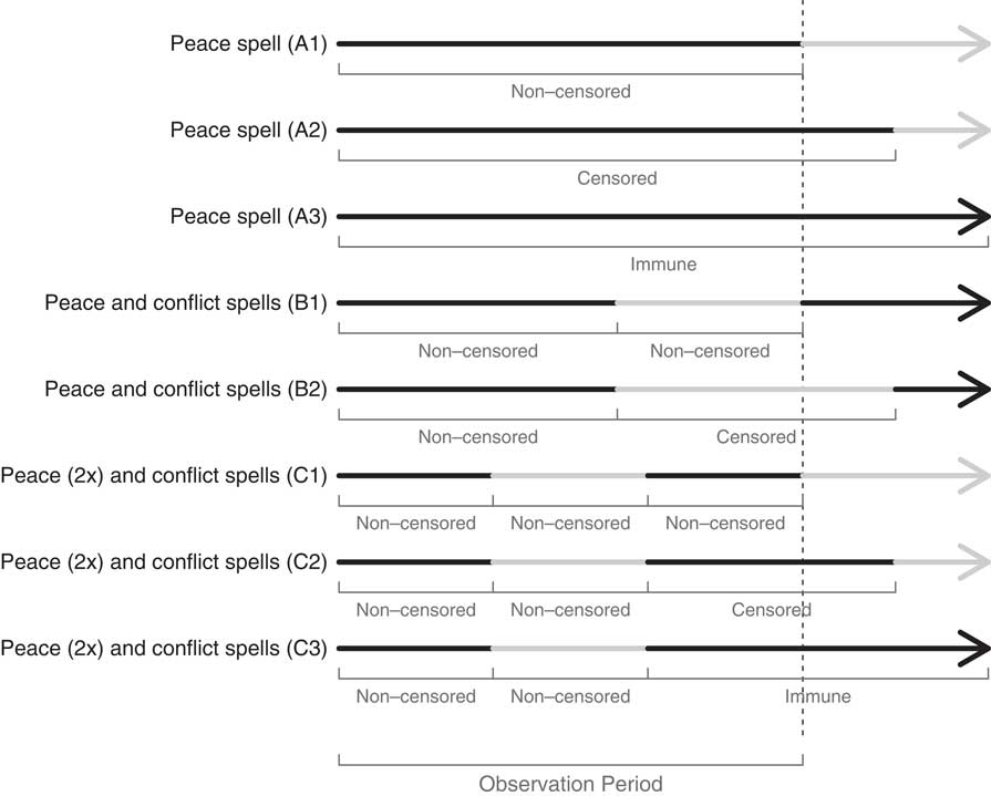
We provide Figure 2 to illustrate the importance of accounting for both strategic independence the immunity of units. Let us assume that we can observe some units (e.g., country) over some observation span (e.g., 67 years if our data run from 1946 through 2004). Let us further assume that, at any given point in time, a unit is in either one of two states: peace or in conflict. Survival analysis treats these units as a series of observations that are “at risk” of an event at every point in time until they experience it. In the first two cases (Figure 2: A1 and A2) the assumption of “at risk” is correct. In case A1 the unit is at peace during the observation period and the peace spell also ends within the observation period. For A2 the assumption of “at risk” also applies even though the end of the peace spell (failure) is outside of our observation period. This is generally called a right-censored observation. However, for the case of A3 the assumption of “at risk” is not met. It will actually never experience failure (conflict) because it is immune. Therefore, we need a SP framework to differentiate between cases like A1/2 and A3.
Conflict data and the differentiation between non-censored, censored, and immune peace spells (black spells) Note: gray lines represent non-censored and censored conflict spells.

However, we not only observe peace spells (A1–A3) but also peace and conflict spells (B1–B2). In cases B1–B2 the “at-risk” assumption holds for both peace and conflict spells because we do not allow for infinite conflict. Two types of events are of our interest here: when a country is currently in peace, then the country is at risk of conflict onset; when the country is currently in conflict, then it is at risk of conflict termination. If a country in one state (peace or conflict) continues to be in the same state by the end of the time unit, we say the country “survives” the time unit. On the other hand, if a country experiences a transition from one state to the other during a time unit t, we say the country experiences a failure at t. In example B1, we observe the full length of the peace (black) and conflict spell (gray), whereas in B2 the conflict spell is right censored but will fail eventually. Thus the main challenge here is not the “immunity” of units but the theoretically implied interdependency between peace and conflict duration.
Finally, we move to examples C1−C3 in Figure 2. They provide a somewhat realistic picture of recurring peace and conflict spells. In the case of C1, we can observe a peace, conflict, and post-conflict peace spell that fails within the observation period. Our theoretical argument proposed that all three spells should be interdependent. This also applies to the cases of C2 and C3. The main difference between C2 and C3 is that the latter case will not revert back to conflict in the future. It is in a sense cured from conflict and will not fail. Thus we have to differentiate between cases C2 where the “at-risk” assumption holds and C3 which violates it.
We thus propose a new empirical framework that allows us to utilize more information contained in the data. We do so by constructing a likelihood function that takes into account the duration of preceding conflict spells in calculating the duration of peace spells and vice versa. Moreover, our proposed model also accommodates the SP technique that estimates the latent probability that a country is “immune” from conflict. This technique, recently introduced to political scientists (e.g., Svolik Reference Svolik2008), is particularly suitable for analyzing conflict data that typically contain long peace periods. We derive this model in several steps. We first introduce simple survival models for peace and conflict duration. We then derive the joint duration model that simultaneously estimates peace and conflict duration. Finally, we present a model that jointly estimates the probability of immunity, as well as peace and conflict duration.
For each of the three models, we provide a general model that allows time-varying covariates. That is, in all of our expositions below, the values of the covariates are allowed to vary within a spell. We do so by splitting each spell into shorter observation periods (e.g., year) such that the values of the covariates are constant within periods but not across periods. Let j=1, … , J s index the observation period within a spell s, where there are J s periods. Let t s,j denote the cumulative duration at period j, where t s,Js is the total duration of spell s. We evaluate the likelihood contribution for each period rather than for each spell.
Part 1: Simple Duration Model
In the standard analysis of peace duration, the likelihood contribution from a unit-period observation that experiences peace survival at time period j is characterized as a conditional probability that peace survives the period j, given peace has survived up to j−1, or
 $$\eqalignno{ {\rm Pr}\left( {T_{s}^{P} \, \gt \, t_{{s, \, j}}^{P} \!\mid\!T_{s}^{P} \, \gt \, t_{{s, \, j \, {\minus} \, 1}}^{P} } \right) & ={{{\rm Pr}\left( {T_{s}^{P} \, \gt \, t_{{s, \, j}}^{P} \, {\cap} \, T_{s}^{P} \, \gt \, t_{{s, \, j \, {\minus} \, 1}}^{P} } \right)} \over {{\rm Pr}\left( {T_{s}^{P} \, \gt \, t_{{s, \, j \, {\minus} \, 1}}^{P} } \right)}} \cr & ={{{\rm Pr}\left( {T_{s}^{P} \, \gt \, t_{{s, \, j}}^{P} } \right)} \over {{\rm Pr}\left( {T_{s}^{P} \, \gt \, t_{{s, \, j \, {\minus} \, 1}}^{P} } \right)}}, $$
where
 $T_{s}^{P} $
is a random variable that represents the duration of peace
spell for s and
 $t_{{s, \, j}}^{P} $
the cumulative duration of peace for s
observed at period j. We treat the observation period
j as right censored (even though the spell
s may not be ultimately right censored at a later period
 $j' \, \gt \, j$
).
On the other hand, the likelihood contribution from an observation that does experience peace failure at period j is given as
 $$\eqalignno{ {\rm Pr}\left( {T_{s}^{P} =t_{{s, \, j}}^{P} \!\mid \!T_{s}^{P} \, \gt \, t_{{s, \, j \, {\minus} \, 1}}^{P} } \right) & ={{{\rm Pr}\left( {T_{s}^{P} =t_{{s, \, j}}^{P} \, {\cap} \, T_{s}^{P} \, \gt \, t_{{s, \, j \, {\minus} \, 1}}^{P} } \right)} \over {{\rm Pr}\left( {T_{s}^{P} \, \gt \, t_{{s, \, j \, {\minus} \, 1}}^{P} } \right)}} \cr & ={{{\rm Pr}\left( {T_{s}^{P} =t_{{s, \, j}}^{P} } \right)} \over {{\rm Pr}\left( {T_{s}^{P} \, \gt \, t_{{s, \, j \, {\minus} \, 1}}^{P} } \right)}}. $$
We then obtain the total likelihood contributions from all the observations in peace spells using the following likelihood function:
 $$L^{P} \propto\prod {\,\left[ {{{{\rm Pr}(T_{s}^{P} \, \gt \, t_{{s, \, j}}^{P} )} \over {{\rm Pr}(T_{s}^{P} \, \gt \, t_{{s, \, j \, {\minus} \, 1}}^{P} )}}} \right]^{{(r_{j} =1)}} \,\left[ {{{{\rm Pr}(T_{s}^{P} =t_{{s, \, j}}^{P} )} \over {{\rm Pr}(T_{s}^{P} \, \gt \, t_{{s, \, j \, {\minus} \, 1}}^{P} )}}} \right]^{{(r_{j} =0)}} ,} $$
where r j is the (period-level) right-censoring indicator that takes a value of 1 for right-censored periods and 0 for non-censored periods.
To further characterize the likelihood function (3), we specify the probability distribution for the duration variable.Footnote 3 Using the flexible Weibull specification,Footnote 4 for example, the density function f(⋅) and the survivor function S(⋅) are each given as a function of the scale parameter λ and the shape parameter α, as follows:Footnote 5
 $$\eqalignno{ & {\rm Pr}\left( {T=t} \right)=\lambda \alpha \left( {\lambda t} \right)^{{(\alpha \, {\minus} \, 1)}} {\rm exp}\left( { {\minus} \left( {\lambda t} \right)^{\alpha } } \right)\,\equiv\,f\left( t \right) \cr & {\rm Pr}\left( {T\gt t} \right)={\rm exp}\left( { {\minus} \left( {\lambda t} \right)^{\alpha } } \right)\,\equiv\,S\left( t \right). $$
The shape parameter determines whether the risk of “failure” event (i.e.,
conflict onset) is increasing (α>1), decreasing
(α<1), or constant (α=1) over
analysis time. We allow the duration of peace to be conditioned on vectors
of time-varying covariates,
 $X_{{sj}}^{P} $
. We do so by specifying the scale parameter governing the
durations as
 $\lambda _{{sj}}^{P} ={\rm exp}( {\minus} X_{{sj}}^{P} \beta ^{P} )$
, where β
P
is the vector of coefficient parameters.
This model takes into account how long peace has survived previously in calculating the likelihood of peace survival and peace failure for each period in the data. It represents a typical duration model employed in the prevalent quantitative studies of conflict onset.Footnote 6 We can also write down a typical model of conflict duration in a similar manner:
 $$L^{C} \propto\prod {\,\left[ {{{{\rm Pr}\left( {T_{s}^{C} \, \gt \, t_{{s, \, j}}^{C} } \right)} \over {{\rm Pr}\left( {T_{s}^{C} \, \gt \, t_{{s, \, j}}^{C} } \right)}}} \right]^{{(r_{j} =1)}} \,\left[ {{{{\rm Pr}\left( {T_{s}^{C} =t_{{s, \, j}}^{C} } \right)} \over {{\rm Pr}\left( {T_{s}^{C} \, \gt \, t_{{s, \, j}}^{C} } \right)}}} \right]^{{(r_{j} =0)}} ,} $$
where
 $T_{s}^{C} $
is a random variable that represents the duration of
conflict for spell s and
 $t_{{s, \, j}}^{C} $
the cumulative duration of conflict for s
observed at period j.
It should be clear from these expositions that a conventional model of peace duration (3) only utilizes information from those observations where conflict is not already ongoing (i.e., cases A1 and A2 in Figure 2), whereas a conventional model of conflict duration (5) focusses only on observations where conflict is already ongoing. If we believe that peace and conflict spells are interdependent, a separate estimation of equations (3) and (5) is inefficient as each model discards information utilized in the other model. In what follows, we present a seemingly unrelated duration model that allows us to estimate these two processes jointly. This is a stepping stone to our proposed SPDDD model.
Part 2: Joint Model of Pre-Conflict Peace, Conflict, and Post-Conflict Peace Duration
The model we present below takes into account the duration of the preceding spells as well as the duration of the present spell up to the observation period. In other words, the duration of post-conflict peace at period j is formulated as a function of its survival up to j−1 as well as the duration of the conflict that precedes it. In this sense, the model is a seemingly unrelated duration model.
Let
 $T_{s}^{{C'}} $
denote a random variable representing the duration of
conflict spell for s that precedes the current peace spell
and
 $t_{s}^{{C'}} $
denote a realization of its value. Then, the likelihood
contribution from a post-conflict peace observation that experiences peace
survival at period j is characterized as a conditional
probability that peace survives j given peace has survived
up to j−1 and the previous conflict has a
duration
 $t_{s}^{{C'}} $
, or
 $$\eqalignno{ {\rm Pr}\left[ {T_{s}^{P} \, \gt \, t_{{s, \, j}}^{P}\! \mid \!\left( {T_{s}^{P} \, \gt \, t_{{s, \, j \, {\minus} \, 1}}^{P} \, {\cap} \, T_{s}^{{C'}} =t_{s}^{{C'}} } \right)} \right] & ={{{\rm Pr}\left( {T_{s}^{P} \, \gt \, t_{{s, \, j}}^{P} \, {\cap} \, T_{s}^{P} \, \gt \, t_{{s, \, j \, {\minus} \, 1}}^{P} \, {\cap} \, T_{s}^{{C'}} =t_{s}^{{C'}} } \right)} \over {{\rm Pr}\left( {T_{s}^{P} \, \gt \, t_{{s, \, j \, {\minus} \, 1}}^{P} \, {\cap} \, T_{s}^{{C'}} =t_{s}^{{C'}} } \right)}} \cr & ={{{\rm Pr}\left( {T_{s}^{P} \, \gt \, t_{{s, \, j}}^{P} \, {\cap} \, T_{s}^{{C'}} =t_{s}^{{C'}} } \right)} \over {{\rm Pr}\left( {T_{s}^{P} \, \gt \, t_{{s, \, j \, {\minus} \, 1}}^{P} \, {\cap} \, T_{s}^{{C'}} =t_{s}^{{C'}} } \right)}}. $$
Similarly, the likelihood contribution from an observation that experiences peace failure at period j is given as
 $$\eqalignno{ {\rm Pr}\left[ {T_{s}^{P} =t_{{s, \, j}}^{P} \!\mid\!\left( {T_{s}^{P} \, \gt \, t_{{s, \, j \, {\minus} \, 1}}^{P} \, {\cap} \, T_{s}^{{C'}} =t_{s}^{{C'}} } \right)} \right] & ={{{\rm Pr}\left( {T_{s}^{P} =t_{{s, \, j}}^{P} \, {\cap} \, T_{s}^{P} \, \gt \, t_{{s, \, j \, {\minus} \, 1}}^{P} \, {\cap} \, T_{s}^{{C'}} =t_{s}^{{C'}} } \right)} \over {{\rm Pr}\left( {T_{s}^{P} =t_{{s, \, j \, {\minus} \, 1}}^{P} \, {\cap} \, T_{s}^{{C'}} =t_{s}^{{C'}} } \right)}} \cr & ={{{\rm Pr}\left( {T_{s}^{P} =t_{{s, \, j}}^{P} \, {\cap} \, T_{s}^{{C'}} =t_{s}^{{C'}} } \right)} \over {{\rm Pr}\left( {T_{s}^{P} \, \gt \, t_{{s, \, j \, {\minus} \, 1}}^{P} \, {\cap} \, T_{s}^{{C'}} =t_{s}^{{C'}} } \right)}}. $$
In addition, we specify the likelihood contribution from conflict
observations at period j as a function of the preceding
peace duration as well as the survival of conflict up to period
j−1. Let
 $T_{s}^{{P'}} $
denote a random variable representing the duration of
peace for s that precedes the current conflict and
 $t_{s}^{{P'}} $
denote its observed value, then we have the following
likelihood function that calculates the total likelihood of the
data:
 $$\eqalignno{ & L\propto\prod {\left[ {{{{\rm Pr}\left( {T_{s}^{P} \, \gt \, t_{{s, \, j}}^{P} } \right)} \over {{\rm Pr}\left( {T_{s}^{P} \, \gt \, t_{{s, \, j \, {\minus} \, 1}}^{P} } \right)}}} \right]^{{(r_{j} =1)}} \left[ {{{{\rm Pr}\left( {T_{s}^{P} =t_{{s, \, j}}^{P} } \right)} \over {{\rm Pr}\left( {T_{s}^{P} \, \gt \, t_{{s, \, j \, {\minus} \, 1}}^{P} } \right)}}} \right]^{{(r_{j} =0)}} } \cr {\rm } & \quad \quad \quad \,\left[ {{{{\rm Pr}\left( {T_{{s, \, j}}^{C} \, \gt \, t_{{s, \, j}}^{C} \, {\cap} \, T_{s}^{{P'}} =t_{s}^{{P'}} } \right)} \over {{\rm Pr}\left( {T_{s}^{C} \, \gt \, t_{{s, \, j}}^{C} \, {\cap} \, T_{s}^{{P'}} =t_{s}^{{P'}} } \right)}}} \right]^{{(r_{j} =1)}} \left[ {{{{\rm Pr}\left( {T_{{s, \, j}}^{C} =t_{{s, \, j}}^{C} \, {\cap} \, T_{s}^{{P'}} =t_{s}^{{P'}} } \right)} \over {{\rm Pr}\left( {T_{s}^{C} \, \gt \, t_{{s, \, j}}^{C} \, {\cap} \, T_{s}^{{P'}} =t_{s}^{{P'}} } \right)}}} \right]^{{(r_{j} =0)}} \cr & \quad \quad \quad \,\left[ {{{{\rm Pr}\left( {T_{s}^{P} \, \gt \, t_{{s, \, j}}^{P} \, {\cap} \, T_{s}^{{C'}} =t_{s}^{{C'}} } \right)} \over {{\rm Pr}\left( {T_{s}^{P} \, \gt \, t_{{s, \, j \, {\minus} \, 1}}^{P} \, {\cap} \, T_{s}^{{C'}} =t_{s}^{{C'}} } \right)}}} \right]^{{(r_{j} =1)}} \left[ {{{{\rm Pr}\left( {T_{s}^{P} =t_{{s, \, j}}^{P} \, {\cap} \, T_{s}^{{C'}} =t_{s}^{{C'}} } \right)} \over {{\rm Pr}\left( {T_{s}^{P} \, \gt \, t_{{s, \, j \, {\minus} \, 1}}^{P} \, {\cap} \, T_{s}^{{C'}} =t_{s}^{{C'}} } \right)}}} \right]^{{(r_{j} =0)}} . $$
The first line in the likelihood function (8) calculates the likelihood contribution from pre-conflict peace spells, the second line from the conflict spells, and the last line from post-conflict peace spells.
A challenge in estimating the likelihood function (8) is to characterize two
types of joint distributions that appear in the likelihood function (8),
namely
 ${\rm Pr}(T^{A} \, \gt \, t^{A} \, {\cap} \, T^{B} =t^{B} )$
and
 ${\rm Pr}(T^{A} =t^{A} \, {\cap} \, T^{B} =t^{B} )$
with
 $(A,B)\in \{ (P,C'),(C,P')\} $
. If the two random variables we have were each Normally
distributed, the joint distribution of the two would simply be a bivariate
Normal. However, both T
A
and T
B
represent duration, which we would want to model with a non-Normal
distribution such as Weibull, log-logistic, or generalized gamma. It is not
straightforward to characterize a joint distribution whose marginal
distributions are not Normal. To deal with this challenge, we utilize a
copula function and derive a new joint distribution from the two duration
variables. A copula is a function that binds together two or more univariate
marginal distributions of known form to produce a new joint distribution
(Trivedi and Zimmer Reference Trivedi and Zimmer2005). Scholars
have used copula functions to construct models of multiple duration
processes (Hays and Kachi Reference Hays and Kachi2011;
Quiroz Flores Reference Quiroz Flores2013), selection
models for duration (Boehmke, Morey and Shannon Reference Boehmke, Morey and Shannon2006; Chiba, Martin and Stevenson Reference Chiba, Martin and Stevenson2015), and joint models of duration and ordered or
count variable (Fukumoto forthcoming; Chiba Reference Chiba2015).
Consider two random variables X and Y with associated univariate distribution functions F X (⋅) and F Y (⋅). Sklar’s (1959) theorem establishes that there exists a copula C( ⋅, ⋅; θ) such that a bivariate joint distribution is defined for all x and y in the extended real line as
 $$F_{{XY}} \left( {x,y} \right)={\rm Pr}\left( {X \, \lt \, x \, {\cap} \, Y \, \lt \, y} \right)=C\left( {F_{X} \left( x \right),F_{Y} \left( y \right);\theta } \right),$$
where the association parameter θ represents the degree of interdependence between x and y. This result is remarkable because it shows that we can construct a new bivariate distribution based on univariate marginal distributions of known form. As long as the univariate marginal distributions are known, an appropriate choice of copula function C(⋅) in (9) enables us to represent the unknown bivariate distribution. Moreover, we can also characterize the density function and the conditional distribution functions using a copula, as follows:
 $$\eqalignno{ f_{{XY}} \left( {x,y} \right)={\rm Pr}\left( {X=x \, {\cap} \, Y=y} \right) & ={{\partial C\left( {F_{X} \left( x \right),F_{Y} \left( y \right);\theta } \right)} \over {\partial x\partial y}} \cr & ={{\partial C\left( {F_{X} \left( x \right),F_{Y} \left( y \right);\theta } \right)} \over {\partial F_{X} \left( x \right)\partial F_{Y} \left( y \right)}} \cdot f_{X} (x) \cdot f_{Y} \left( y \right) \cr f_{{X\,\mid\,Y}} \left( {x,y} \right)={\rm Pr}\left( {X=x\!\mid\! Y=y} \right) & ={{{\rm Pr}\left( {X=x \, {\cap} \, Y=y} \right)} \over {{\rm Pr}\left( {Y=y} \right)}}={{f_{{XY}} \left( {x,y} \right)} \over {f_{Y} \left( y \right)}}, \cr F_{{X\,\mid\,Y}} \left( {x,y} \right)={\rm Pr}\left( {X \, \lt \, x\!\mid\!Y=y} \right) & =\mathop{\int}\limits_{ \, {\minus} \infty}^x {f_{{X\,\mid\,Y}} \left( {x,y} \right)} , $$
where f X (⋅) and f Y (⋅) are the univariate density functions for X and Y.
With these functions, we can thus specify the first type of joint probability in (8) as
 $$\eqalignno{ {\rm Pr}\left( {T^{A} \, \gt \, t^{A} \, {\cap} \, T^{B} =t^{B} } \right) & ={\rm Pr}\left( {T^{B} =t^{B} } \right) \, {\minus} \, {\rm Pr}\left( {T^{A} \, \lt \, t^{A} \, {\cap} \, T^{B} =t^{B} } \right) \cr & ={\rm Pr}\left( {T^{B} =t^{B} } \right) \cdot \left[ {1 \, {\minus} \, {{{\rm Pr}\left( {T^{A} \, \lt \, t^{A} \, {\cap} \, T^{B} =t^{B} } \right)} \over {{\rm Pr}\left( {T^{B} =t^{B} } \right)}}} \right] \cr & ={\rm Pr}\left( {T^{B} =t^{B} } \right) \cdot \left[ {1 \, {\minus} \, {\rm Pr}\left( {T^{A} \, \lt \, t^{A} \\mid\T^{B} =t^{B} } \right)} \right] \cr & =f_{Y} \left( {t^{B} } \right) \cdot \left[ {1 \, {\minus} \, F_{{X\,\mid\,Y}} \left( {t^{A} ,t^{B} } \right)} \right], $$
where f(⋅) is the density function for duration (e.g., Weibull as defined in (4)). The second type of joint probability in (8) is obtained simply as
 $${\rm Pr}\left( {T^{A} =t^{A} \, {\cap} \, T^{B} =t^{B} } \right)=f_{{XY}} \left( {t^{A} ,t^{B} } \right).$$
To complete the derivation, the last step is to choose a particular copula function for C(⋅ , ⋅; θ) to characterize functions in (9) and (10). There are a number of different copula functions that can be used to construct a multivariate distribution from univariate marginals (Trivedi and Zimmer Reference Trivedi and Zimmer2005), but some copulas are more flexible than others in that they can accommodate greater range of dependency between the marginals. In this study, we use the Gaussian copula, one of the most flexible copula functions that can accommodate both positive and negative dependency. It has the following form:
 $$C\left( {u,v;\theta } \right)=\mathop{\int}\limits_{ \, {\minus} \, \infty}^{{\rm \Phi }^{{ \, {\minus} 1}} (u)} \,\mathop{\int}\limits_{ \, {\minus} \, \infty}^{{\rm \Phi }^{{ \, {\minus} 1}} (v)} {{1 \over {2\pi \left( {1 \, {\minus} \, \theta ^{2} } \right)^{{1/2}} }}} \,{\rm exp}\left[ {{{ \, {\minus} \left( {s^{2} \, {\minus} \, 2\theta st{\plus}t^{2} } \right)} \over {2\left( {1 \, {\minus} \, \theta ^{2} } \right)}}} \right]dsdt,$$
where Φ−1() is the Gaussian quantile function, −1<θ<1 is the association parameter, and u=F x (x) and v=F y (y) for random variables x and y. With the Gaussian copula, the density and the conditional functions in (10) have the following forms:
 $$\eqalignno{ & f_{{XY}} \left( {x,y} \right)=\left( {1 \, {\minus} \, \theta ^{2} } \right)^{{ {\minus} {1 \over 2}}} {\rm exp}\left[ { \, {\minus} \, {1 \over 2}\left( {1 \, {\minus} \, \theta ^{2} } \right)^{{ {\minus} 1}} \left( {a^{2} {\plus}b^{2} \, {\minus} \, 2\theta ab} \right)} \right]{\rm exp}\left[ {{1 \over 2}\left( {a^{2} {\plus}b^{2} } \right)} \right] \cdot f_{X} \left( x \right) \cdot f_{Y} \left( y \right) \cr & F_{{X\,\mid\,Y}} \left( {x,y} \right)=\mathop{\int}\limits_{ \, {\minus} \, \infty}^a {f_{{XY}} \left( {x,y} \right)={\rm \Phi }\left( {{{a \, {\minus} \, \theta b} \over {\sqrt {1 \, {\minus} \, \theta ^{2} } }}} \right)} , $$
where a=Φ −1(F X (x)), b=Φ−1(F Y (y)), and Φ(⋅) is the standard Normal distribution function.
The Gaussian copula has a number of desirable characteristics. First, it allows for independence as a special case (θ=0). We can thus test the existence of interdependence between the two processes by testing whether θ is different from 0. Second, the Gaussian copula is comprehensive in that as θ approaches the lower (upper) bound of its permissible range, the copula approaches the theoretical lower (upper) bound.Footnote 7 Third, the derivation of the conditional functions in (10) is straightforward with the Gaussian copula.
Bringing it Together: An SPDDD Model
We further extend this joint model by incorporating the SP technique that allows us to split the observations into those that are “immune” from conflict and those that are not. This technique has been developed in medical research where researchers are interested in identifying those patients that are cured of a disease of interest (and hence not at risk of death from the said disease) and those that are still at risk. When a patient dies of the disease at a given period, researchers know with certainty that the patient has not been cured of the disease. When a patient survives a given period, however, one must consider two possibilities: the patient is cured of the disease of interest, or the patient is not cured but his/her time has not come at the period yet. As “cure” is unobservable, an SP model estimates the latent probability that a patient is cured or not.
We apply this technique to the study of peace and conflict by specifying the probability that a country is “immune” from conflict. In the context of conflict research, we can think of immunity as a situation where actors are satisfied with the status quo. According to the bargaining perspective, unsatisfied actors (i.e., those that are not immune from conflict) can, nevertheless, avoid war if they can agree to a bargain that makes both sides better off than costly fighting. The disputants’ ability to find such mutually beneficial agreements, however, is severely constrained in the presence of informational problems or commitment problems (Fearon Reference Fearon1995; Powell Reference Powell2006). We would expect that these problems generally grow over time, as there will be a greater chance that some exogenous shocks create sources of the bargaining problem. It may be the case that one party’s military power grows faster than that of the other disputing party, which creates dynamic commitment problems. It may also be the case that the convergence of expectations with regard to the fighting capabilities of one another get distorted, creating informational problems. As the bargaining problem grows severer over time, the conditional risk of conflict onset given non-immunity should also grow over time, whereas the risk of conflict onset remains zero for immune countries (those that do not have issues to fight over in the first place). SP technique allows us to capture this dynamic by estimating the likelihood of immunity and the conditional risk of conflict given non-immunity.
Let c s,j denote a binary indicator that takes the value of 1 whenever a country is “immune” from conflict, and 0 if a country is at risk of conflict. As we do not observe whether the right-censored country-period observations s,j in the data are immune or not, c s,j is an unobservable variable. When an observation in a peace spell survives period j, the country may be either totally immune from conflict or non-immune (but its time has not come). Then, the likelihood contribution from an observation that experiences peace survival at period j is a combination of the likelihood that an observation is immune from conflict and the likelihood that an observation is not immune but has not experienced conflict during that period. We can thus rewrite equation (6) as follows:
 $$\eqalignno{ {\rm Pr}\left[ {\left\{ {c_{{s, \, j}} =1{\cup}\left( {c_{{s, \, j}} =0 \, {\cap} \, T_{s}^{P} \, \gt \, t_{{s, \, j}}^{P} } \right)} \right\}\,\mid\,\left\{ {c_{{s, \, j}} =1{\cup}\left( {c_{{s, \, j}} =0 \, {\cap} \, T_{s}^{P} \, \gt \, t_{{s, \, j \, {\minus} \, 1}}^{P} \, {\cap} \, T_{s}^{{C'}} =t_{s}^{{C'}} } \right)} \right\}} \right] \cr \quad \quad \quad \;={{{\rm Pr}\left[ {c_{{s, \, j}} =1{\cup}\left( {c_{{s, \, j}} =0 \, {\cap} \, T_{s}^{P} \, \gt \, t_{{s, \, j}}^{P} \, {\cap} \, T_{s}^{{C'}} =t_{s}^{{C'}} } \right)} \right]} \over {{\rm Pr}\left[ {c_{{s, \, j}} =1{\cup}\left( {c_{{s, \, j}} =0 \, {\cap} \, T_{s}^{P} \, \gt \, t_{{s, \, j \, {\minus} \, 1}}^{P} \, {\cap} \, T_{s}^{{C'}} =t_{s}^{{C'}} } \right)} \right]}} \cr \quad \quad \quad \;={{{\rm Pr}\left( {c_{{s, \, j}} =1} \right){\plus}{\rm Pr}\left( {c_{{s, \, j}} =0} \right){\rm Pr}\left[ {\left( {T_{s}^{P} \, \gt \, t_{{s, \, j}}^{P} \, {\cap} \, T_{s}^{{C'}} =t_{s}^{{C'}} } \right) \!\mid \!c_{{s, \, j}} =0} \right]} \over {{\rm Pr}\left( {c_{{s, \, j}} =1} \right){\plus}{\rm Pr}\left( {c_{{s, \, j}} =0} \right){\rm Pr}\left[ {\left( {T_{s}^{P} \, \gt \, t_{{s, \, j \, {\minus} \, 1}}^{P} \, {\cap} \, T_{s}^{{C'}} =t_{s}^{{C'}} } \right)\!\mid\!c_{{s, \, j}} =0} \right]}}, $$
where
 ${\rm Pr}[(T_{s}^{P} \, \gt \, t_{{s, \, j}}^{P} \, {\cap} \, T_{s}^{{C'}} =t_{s}^{{C'}} ) \!\mid\!c_{{s, \, j}} =0]$
is the conditional joint probability of post-conflict
peace survival and conflict duration given non-immunity.
On the other hand, when an observation in a peace spell experiences conflict, the country must be non-immune and c s,j =0. To calculate the likelihood contribution from such an observation, we rewrite equation (7) as follows:
 $$\eqalignno{ {\rm Pr}\left[ {c_{{s, \, j}} =0 \, {\cap} \, T_{s}^{P} =t_{{s, \, j}}^{P} \,\mid\,\left\{ {c_{{s, \, j}} =1{\cup}\left( {c_{{s, \, j}} =0 \, {\cap} \, T_{s}^{P} \, \gt \, t_{{s, \, j \, {\minus} \, 1}}^{P} \, {\cap} \, T_{s}^{{C'}} =t_{s}^{{C'}} } \right)} \right\}} \right] \cr \;\;\;={{{\rm Pr}\left[ {c_{{s, \, j}} =0 \, {\cap} \, T_{s}^{P} =t_{{s, \, j}}^{P} \, {\cap} \, T_{s}^{{C'}} =t_{s}^{{C'}} } \right]} \over {{\rm Pr}\left[ {c_{{s, \, j}} =1{\cup}\left( {c_{{s, \, j}} =0 \, {\cap} \, T_{s}^{P} \, \gt \, t_{{s, \, j \, {\minus} \, 1}}^{P} \, {\cap} \, T_{s}^{{C'}} =t_{s}^{{C'}} } \right)} \right]}} \cr \;\;\;={{{\rm Pr}\left( {c_{{s, \, j}} =0} \right){\rm Pr}\left[ {\left( {T_{s}^{P} =t_{{s, \, j}}^{P} \, {\cap} \, T_{s}^{{C'}} =t_{s}^{{C'}} } \right)\,\mid\,c_{{s, \, j}} =0} \right]} \over {{\rm Pr}\left( {c_{{s, \, j}} =1} \right){\plus}{\rm Pr}\left( {c_{{s, \, j}} =0} \right){\rm Pr}\left[ {\left( {T_{s}^{P} \, \gt \, t_{{s, \, j \, {\minus} \, 1}}^{P} \, {\cap} \, T_{s}^{{C'}} =t_{s}^{{C'}} } \right)\,\mid\,c_{{s, \, j}} =0} \right]}}, $$
where
 ${\rm Pr}[(T_{s}^{P} =t_{{s, \, j}}^{P} \, {\cap} \, T_{s}^{{C'}} =t_{s}^{{C'}} )\!\mid\!c_{{s, \, j}} =0]$
is the conditional joint probability density of
post-conflict peace duration given non-immunity.
Our proposed model thus has the following likelihood function:
 $$\eqalignno{ & L\propto\prod {\left[ {{{{\rm Pr}\left( {c_{{s, \, j}} =1} \right){\plus}{\rm Pr}\left( {c_{{s, \, j}} =0} \right){\rm Pr}\left( {T_{s}^{P} \, \gt \, t_{{s, \, j}}^{P} \,\mid\,c_{{s, \, j}} {\rm =}0} \right)} \over {{\rm Pr}\left( {c_{{s, \, j}} =1} \right){\plus}{\rm Pr}\left( {c_{{s, \, j}} =0} \right){\rm Pr}\left( {T_{s}^{P} \, \gt \, t_{{s, \, j \, {\minus} \, 1}}^{P} \,\mid\,c_{{s, \, j}} {\rm =}0} \right)}}} \right]^{{(r_{j} =1)}} } \cr {\rm } & \quad \quad \quad \,\left[ {{{{\rm Pr}\left( {c_{{s, \, j}} =0} \right){\rm Pr}\left( {T_{s}^{P} =t_{{s, \, j}}^{P} \,\mid\,c_{{s, \, j}} =0} \right)} \over {{\rm Pr}\left( {c_{{s, \, j}} =1} \right){\plus}{\rm Pr}\left( {c_{{s, \, j}} =0} \right){\rm Pr}\left( {T_{s}^{P} \, \gt \, t_{{s, \, j \, {\minus} \, 1}}^{P} \,\mid\,c_{{s, \, j}} =0} \right)}}} \right]^{{(r_{j} =0)}} \cr {\rm } & \quad \quad \quad \,\left[ {{{{\rm Pr}\left( {T_{{s, \, j}}^{C} \, \gt \, t_{{s, \, j}}^{C} \, {\cap} \, T_{s}^{{P'}} =t_{s}^{{P'}} } \right)} \over {{\rm Pr}\left( {T_{s}^{C} \, \gt \, t_{{s, \, j}}^{C} \, {\cap} \, T_{s}^{{P'}} =t_{s}^{{P'}} } \right)}}} \right]^{{\left( {r_{j} =1} \right)}} \left[ {{{{\rm Pr}\left( {T_{{s, \, j}}^{C} =t_{{s, \, j}}^{C} \, {\cap} \, T_{s}^{{P'}} =t_{s}^{{P'}} } \right)} \over {{\rm Pr}\left( {T_{s}^{C} \, \gt \, t_{{s, \, j}}^{C} \, {\cap} \, T_{s}^{{P'}} =t_{s}^{{P'}} } \right)}}} \right]^{{(r_{j} =0)}} \cr {\rm } & \quad \quad \quad \,\left[ {{{{\rm Pr}\left( {c_{{s, \, j}} =1} \right){\plus}{\rm Pr}\left( {c_{{s, \, j}} =0} \right){\rm Pr}\left[ {\left( {T_{s}^{P} \, \gt \, t_{{s, \, j}}^{P} \, {\cap} \, T_{s}^{{C'}} =t_{s}^{{C'}} } \right)\,\mid\,c_{{s, \, j}} =0} \right]} \over {{\rm Pr}\left( {c_{{s, \, j}} =1} \right){\plus}{\rm Pr}\left( {c_{{s, \, j}} =0} \right){\rm Pr}\left[ {\left( {T_{s}^{P} \, \gt \, t_{{s, \, j \, {\minus} \, 1}}^{P} \, {\cap} \, T_{s}^{{C'}} =t_{s}^{{C'}} } \right)\,\mid\,c_{{s, \, j}} =0} \right]}}} \right]^{{(r_{j} =1)}} \cr {\rm } & \quad \quad \quad \,\left[ {{{{\rm Pr}\left( {c_{{s, \, j}} =0} \right){\rm Pr}\left[ {\left( {T_{s}^{P} =t_{{s, \, j}}^{P} \, {\cap} \, T_{s}^{{C'}} =t_{s}^{{C'}} } \right)\,\mid\,c_{{s, \, j}} =0} \right]} \over {{\rm Pr}\left( {c_{{s, \, j}} =1} \right){\plus}{\rm Pr}\left( {c_{{s, \, j}} =0} \right){\rm Pr}\left[ {\left( {T_{s}^{P} \, \gt \, t_{{s, \, j \, {\minus} \, 1}}^{P} \, {\cap} \, T_{s}^{{C'}} =t_{s}^{{C'}} } \right)\,\mid\,c_{{s, \, j}} =0} \right]}}} \right]^{{(r_{j} =0)}} , $$
where the first two lines calculate the likelihood
contribution from pre-conflict peace observations, the third line from
conflict observations, and the last two lines from post-conflict peace
observations. We let c
s,j
be a function of covariates,
 $X_{{s, \, j}}^{I} $
, and use a logit link function such that
 ${\rm Pr}(c_{{s, \, j}} =1)=\left( {1{\plus}{\rm exp}( \, {\minus} \, X_{{s, \, j}}^{I} \beta ^{I} )} \right)^{{ \!{\minus} 1}} $
. Therefore, we estimate four equations jointly: one for
pre-conflict peace duration, one for conflict duration, one for
post-conflict peace duration, and one for immunity.
MONTE CARLO SIMULATION
We demonstrate the performance of this model via Monte Carlo simulations. The analysis reveals that the conventional survival model that ignores immunity status produces biased estimates of the model parameters, even when there is no interdependence between peace and conflict processes. It also shows that, when the processes underlying peace and conflict durations are non-trivially correlated, the SPDDD model outperforms the conventional SP model that estimates peace and conflict durations separately.
A single round of our Monte Carlo simulation consists of 1000 hypothetical country-conflict observations. Each country-conflict has at most three spells: pre-conflict peace spell, conflict spell, and post-conflict peace spell. However, for those observations that are “immune” from conflict, we only observe pre-conflict peace spells. To illustrate the performance of models that recognize the interdependence between peace and conflict, we vary the value of θ from −0.9 (very high negative interdependence between peace and conflict) to 0.9 (very high positive interdependence) with an increment of 0.1. We perform 200 simulations for a given value of θ.
We assume four independent variables influence the process, x 1, x 2, x 3, and x 4. x 1 influences the duration of peace (both pre-conflict and post-conflict), x 2 influences the duration of conflict, and x 3 and x 4 influence the latent immunity status. We generate 1000 values of these four variables, each according to an independent uniform distribution over (−3,3). We hold these variables constant throughout the simulations.
Each round of simulation begins by generating a latent immunity status for each
country-conflict i,
 $c_{i}^{{\rm {\asterisk}}} $
, according to the following specification:
 $$c_{i}^{{\asterisk}} {\rm =} \, {\minus} \, x_{3} {\rm {\plus}}x_{4} {\rm {\plus}}\eta _{i} ,$$
where η
i
follows a logistic distribution. Those observations where
 $c_{i}^{{\rm {\asterisk}}} \, \gt \, 0$
are immune from conflict and those where
 $c_{i}^{{\rm {\asterisk}}} \leq 0$
are at risk of conflict. On average, 50 percent of the
observations are immune. We then generate two correlated random variables
(ν
P
,ν
C
) for each of the 1000 observations according to a bivariate Normal
distribution with a given correlation coefficient θ. To
generate peace and conflict durations, we transform ν
m
, m∈{P,C} into a
Weibull variate ϵ
m
using the inverse transformation method such that ϵ
m
=−log(1−Φ(ν
m
)).Footnote
8
Then, we generate peace and conflict duration t
m
as
 $$\eqalignno{ & t_{P} {\rm =exp}\left( {x_{1} } \right){\plus}\epsilon _{P} \cr & t_{C} {\rm =exp}\left( {x_{2} } \right){\plus}\epsilon _{C} . $$
For those observations that are immune from conflict (i.e., c i >0), (1) the pre-conflict peace duration is replaced with a larger value (i.e., the maximum value of t P in a given round of simulation), (2) the pre-conflict peace is treated as right censored, and (3) conflict and post-conflict peace durations are dropped.
For each set of data, we estimate four sets of models: (1) a simple duration model of peace (pre conflict and post conflict) and conflict, (2) a seemingly unrelated duration model of peace and conflict, (3) SP model of peace, and (4) our developed model, an SPDDD model of peace and conflict. For all of the models, we specify the right-hand side of the equations as follows:
 $$\eqalignno{ & {\rm pre{\hyphen}conflict}\,{\rm peace=}\, \beta _{{P0}} {\rm {\plus}}\beta _{{P1}} {\times}x_{1} {\plus}\beta _{{P2}} {\times}x_{3} \cr & {\rm conflict=}\, \beta _{{C0}} {\rm {\plus}}\beta _{{C1}} {\times}x_{2} \cr & {\rm post{\hyphen}conflict}\,{\rm peace=}\, \beta _{{PC0}} {\rm {\plus}}\beta _{{PC1}} {\times}x_{1} {\rm {\plus}}\beta _{{PC2}} {\times}x_{3} \cr & {\rm immunity=}\, \beta _{{I0}} {\rm {\plus}}\beta _{{I1}} {\times}x_{3} {\rm {\plus}}\beta _{{I2}} {\times}x_{4} . $$
We are particularly interested in the estimates of β P2. As x 3 only influences the immunity status but not the peace duration in the data-generating process, the true value of β P2 is 0. As we will show below, however, models that ignore immunity status will produce estimates far from 0 even in the absence of the interdependence between peace and conflict durations. On the other hand, SP models recover values very close to 0, on average. Furthermore, when there is a non-negligible amount of interdependence between the two duration processes, the seemingly unrelated duration model outperforms the regular SP duration models in terms of root mean squared errors (RMSEs).
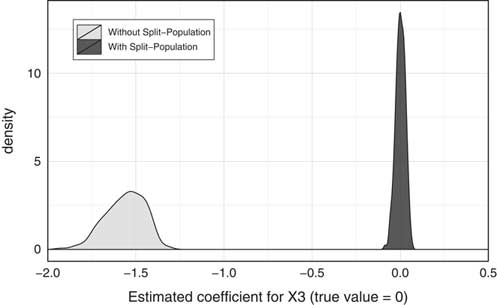
We first show the comparison between models with and without an SP component. Figure 3 shows the estimated values of β P2 from four models when there is no interdependence between two durations (θ=0). The density to the left of the figure (in light gray) shows the estimates from the models without SP component (simple duration model and seemingly unrelated duration model).Footnote 9 The density to the right of the figure (in dark gray) shows the estimates from the models with an SP component (standard SP duration model and our proposed SPDDD model).Footnote 10 We can see that both a standard SP duration and SPDDD models successfully recover the true value of β P2, whereas those without an SP component systematically underestimate it. This is because x 3 negatively influences the immunity status in the data-generating process, as shown in equation (17). As non-immune observations have shorter durations of peace than immune observations, models that ignore the immunity status mistakenly attribute the negative effect of x 3 on immunity to the negative effect of x 3 on peace duration.
Bias in estimation Note: this figure displays the estimated coefficient for x 3 in the pre-conflict peace duration, or β P2 in equation (18). The density in light gray to the left of the figure shows the estimates from models without a split-population (SP) component, whereas the density in dark gray to the right of the figure shows the estimates from models with an SP component (standard SP model and our proposed SPDDD model). The figure shows that the estimates from models with an SP component are centered around the true value of β P2(=0) but those from models without it are negatively biased.

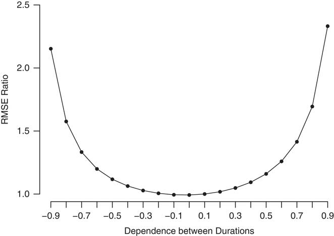
What would happen if there exists an interdependence between peace and conflict durations, as our theoretical argument suggests? To illustrate the inefficiency of an approach that ignores the interdependence, we compare our SPDDD model with the simple SP model that estimates peace and conflict durations separately. Although both models successfully recover the true values, on average, the simple SP model produces greater amount of estimation errors than does the SPDDD model. Figure 4 shows the ratio of RMSE from the two models for different values of interdependence between durations (θ). Specifically, it shows the RMSE from the SP model divided by the RMSE from the SPDDD model where we vary the value of θ from −0.9 (very high negative dependence) to 0.9 (very high positive dependence). When the two models produce equivalent amount of estimation errors, the ratio is equal to 1. The ratio will be >1 when the SP model produces greater average error compared with the SPDDD model. As we can see in the figure, as θ gets bigger in absolute values, the SP model produces much larger RMSE compared with the SPDDD model.
Efficiency in estimation Note: this figure shows the ratio of root mean squared error (RMSE) for the simple split-population (SP) model and the split-population duration-duration-duration (SPDDD) model across different values of interdependence between durations. The X-axis denotes the amount of interdependence (θ, varying from −0.9 to 0.9) and the Y-axis shows the RMSE from the SP model divided by the RMSE from the SPDDD model. We can see that, as θ moves away from 0, the SP model produces larger RMSE compared with the SPDDD model.

AN EMPIRICAL APPLICATION
We now turn to an empirical application of our approach to historical data on intrastate conflict from 1946 through 2004. Our sample consists of all independent states as compiled by Gleditsch and Ward (Reference Gleditsch and Ward1999).Footnote 11 During this period, 177 countries are recognized as independent states. We limit our focus to 166 countries for which reliable information is available at some point during this period.Footnote 12 We use information from the UCDP data sets to code intrastate conflict,Footnote 13 99 countries in our sample (59 percent) have experienced at least one intrastate conflict during the observation span, whereas 67 countries (41 percent) have never experienced intrastate conflict.
Peace and Conflict Spells
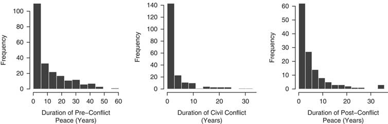
There are 222 unique conflict spells during the observation span. We define conflict spells as a series of country-day observations where a country experiences at least one ongoing intrastate conflict.Footnote 14 The duration of a conflict spell is calculated as the number of days elapsed since the onset of intrastate conflict until its termination or the end of the observation span, December 31, 2004. In our data, there are 19 conflict spells (8.6 percent) where intrastate conflict was still ongoing as of the end date of the observation span. These conflict spells are treated as right censored on December 31, 2004.Footnote 15 Therefore, the actual date of conflict termination is observed for the remaining 203 non-censored conflict spells. The duration of conflict spells for the non-censored ones ranges from 1 day to 11,322 days (31 years).Footnote 16 The histogram in the middle panel in Figure 5 shows the distribution of conflict duration for the 203 non-censored conflict spells.
Duration of peace and civil conflict, 1946–2004 Note: the histogram to the left shows the duration of pre-conflict peace (in years) for the non-censored spells (n=222). The histogram in the middle shows the duration of intrastate conflict (in years) for the non-censored conflict spells (n=203). The histogram to the right shows the duration of post-conflict peace (in years) for the non-censored spells (n=129).

For each of the terminated (i.e., non-censored) conflict spells, we calculate the duration of post-conflict peace. A post-conflict peace spell is a series of country-day observations where a country is not experiencing an intrastate conflict. It starts with the termination of an intrastate conflict. As there are 203 non-censored conflict spells, there are 203 post-conflict peace spells. The duration of a post-conflict peace spell is calculated as the number of days elapsed since the termination date of the preceding conflict spell until either one of the following three dates, whichever comes first: (1) the date when another intrastate conflict begins in a country (129 spells or 63 percent); (2) the date when the country lost its independence (two spells or 1 percent); or (3) December 31, 2004 (72 spells or 35 percent).Footnote 17 The latter two types of post-conflict spells are treated as right censored. The actual end date of a post-conflict peace spell is observed for the 129 non-censored post-conflict peace process that ended with a recurrence of conflict. The duration of post-conflict spells for the non-censored ones ranges from 1 day to 12,694 days (35 years).Footnote 18 The histogram in the right panel in Figure 5 shows the distribution of post-conflict peace duration for the 129 non-censored spells.
Finally, we define pre-conflict peace spells for all the 222 conflict spells as well as for the 63 countries that did not experience any intrastate conflict during the observation span, yielding a sample of 285 pre-conflict peace spells. The starting date of a pre-conflict peace spell is the latest date of the following three dates: (1) the date of termination of the most recent intrastate conflict; (2) the date of independence; or (3) January 1, 1946. The exact duration of a pre-conflict peace spell can be determined only if we get to observe an onset of intrastate conflict. An intrastate conflict breaks out in 222 pre-conflict peace spells (78 percent). For the remaining spells, we observe the duration of peace up until December 31, 2004 (61 spells or 21 percent) or the date when the country lost its independence (two spells or 1 percent).Footnote 19 We treat these spells as right censored. For the 222 non-censored spells, the duration ranges from 1 day to 20,343 days (56 years).Footnote 20 The histogram on the left side in Figure 5 shows the distribution of pre-conflict peace duration for the non-censored spells.
As most of the covariates we introduce below change their values annually, we divide each of the spells into multiple spell-year observations. There are 5370 pre-conflict spell-years (285 pre-conflict spells), 1076 conflict spell-years (222 conflict spells), and 2179 post-conflict spell-years (203 post-conflict spells) in the data.
Covariates
We test the empirical implications of our theoretical argument with a set of variables measuring the characteristics of peace and conflict spells. Before turning to the specification for the duration equations, we present the covariates in the immunity equation. Remember that we argued that satisfied actors are unlikely to begin fighting and hence contribute to immune peace spells. We argued that economic development is associated with satisfied actors and use GDP per capita and controlling for Population to capture this idea. These variables are taken from Fearon and Laitin (Reference Fearon and Laitin2003) and Bleaney and Dimico (Reference Bleaney and Dimico2011). We also argued that anocracies are not able to address the needs of unsatisfied actors (like stable democracies) nor can they induce the costs to violence (like stable autocracies). We compose the X-Polity score according to Vreeland (Reference Vreeland2008), taking the original Polity case format data (Marshall, Gurr and Jaggers Reference Marshall, Gurr and Jaggers2014) and include the squared term to model the implied curvilinear relationship. Finally, we prepare a dummy variable 1+ excluded that codes whether one or more ethnic groups are excluded from power, as we argued that policies that create gaps between the underlying and actual power distribution are bound to create unsatisfied actors. The data are taken from Cederman, Wimmer and Min (Reference Cederman, Wimmer and Min2010).
Theoretically, we are less interested in the specification of the duration equations. This is because our theoretical argument focusses on the importance of unobserved factors. Thus, the main concern is a well-specified model that captures important factors contributed to pre-conflict, conflict, and post-conflict duration.
For conflict spell-years, we use the following covariates. Multilateral conflict takes a value of 1 for conflict spell-years where the government fights with more than one rebel groups, and 0 otherwise. Specifically, this variable is coded 1 when (1) the government fights more than one intrastate conflicts in a given spell-year or (2) the government fights more than one rebel groups in one intrastate conflict in a given spell-year. We rely on information from the UCDP Armed Conflict data set (the Side B variable) in coding this variable and want to capture the robust finding that multiple actors are related to longer conflict duration (Cunningham Reference Cunningham2006). Conflict over territory takes the value of 1 for conflict spell-years where the incompatible positions between the government and rebel only concerns territory, and 0 otherwise. We use the Incompatibility variable from the UCDP data set to code these variables, which pertains to the idea that territorial aspects matter for conflict duration (Buhaug, Gates and Lujala Reference Buhaug, Gates and Lujala2009). Intensity is also found to be an important predictor of conflict duration (Regan Reference Regan2002) and is coded 1 for spell-years where the levels of violence exceed the threshold of a civil war according to the UCDP data set. We control for excluded ethnic groups (1+ excluded groups) in line with empirical support for the notion that ethnic exclusion impacts on conflict duration (Wucherpfennig et al. Reference Wucherpfennig, Metternich, Cederman and Gleditsch2012). Resources are frequently argued to affect conflict dynamics and we control for the occurrence of Diamonds and on-shore Oil. We also account for the political institutions (X-Polity) and whether the conflict has taken place during the Cold War.
For pre-conflict peace spells we introduce a similar set of covariates as in the immunity equation. We do this because the current literature does not systematically distinguish between factors that contribute to the immunity of conflict or the length of peace spell in at-risk cases. However, we argue that lootable resources can lead to a quicker onset of fighting if a country is at risk of conflict. Hence, our model includes Diamonds and on-shore Oil coded 1 for countries with such and 0 otherwise. More generally, the main explanatory variables that we introduce in the immunity and pre-conflict duration equation are similar to the main explanatory variables in civil conflict onset studies (Hegre et al. Reference Hegre, Ellingsen, Gates and Gleditsch2001; Fearon and Laitin Reference Fearon and Laitin2003; Cederman, Wimmer and Min Reference Cederman, Wimmer and Min2010).
Finally, for post-conflict peace spells we especially focus on the outcome of the previous conflict. It is frequently argued that especially government victories increase the duration of post-conflict peace and empirical support for this argument seems to be robust (Toft Reference Toft2010). We use information from the UCDP Conflict Termination Data set to code how the preceding conflict is terminated. Government victory takes the value of 1 for post-conflict peace spells where the preceding conflict ends in government victory, and 0 for non-post-conflict peace spells and post-conflict peace spells where the preceding conflict does not end in government victory. Rebel victory takes the value of 1 for post-conflict peace spells where the preceding conflict ends in rebel victory, and 0 for non-post-conflict peace spells and post-conflict peace spells where the preceding conflict does not end in rebel victory. Finally, Peace/ceasefire agreements takes the value of 1 for post-conflict peace spells where the disputing parties ends the preceding conflict with either a peace agreement or a ceasefire agreement. This leaves No/Low Intensity outcomes as the baseline category. We also control for regime type (X-Polity, economic development (per capita GDP), Population, and natural resources (Oil coded 1 for countries with on-shore oil wells and 0 otherwise, Diamond coded 1 for countries with diamond mines and 0 otherwise). Finally, we account for politically excluded ethnic groups in the post-conflict peace period (1+ excluded groups).
We impute the missing values of the structural variables using the semi-parametric imputation technique proposed by Hoff (Reference Hoff2007).
EMPIRICAL RESULTS
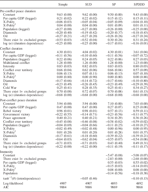
Table 2 shows the estimated coefficients from four models. The first column reports the results from a simple duration model of peace and conflict.Footnote 21 These results correspond to the results typically reported in conflict research that assumes as if the two processes were unrelated. The second column reports the results from a seemingly unrelated duration model of peace and conflict that recognizes the interdependence between peace and conflict, whereas still ignoring immunity status. The third column reports the results from a simple SP model that accounts for immunity but ignores the interdependence. Finally, the fourth column reports the results from our SPDDD model. We can assess the relative performance of these models by comparing Akaike Information Criterion (AIC) scores from each model, as the first model is nested in the second, third, and fourth models and the second and third models are each nested in the fourth model. We can see that our SPDDD model yields the lowest AIC score of all the four models, suggesting that it fits the data better than the other three models.
Results from Four Different Models

Note: SP, split population; SPDDD, split-population duration-duration-duration; AIC, Akaike Information Criterion.
p-values (two-tailed test) in parentheses.
As we noted previously, two parametric specifications are used to describe the duration processes of peace and conflict: Weibull parametrization and log-logistic parametrization. Weibull parametrization is a simple and flexible specification where the underlying failure risk (i.e., hazard) is allowed to increase, decrease, or be constant. One limitation of the Weibull specification, however, is that it does not allow for non-monotonic change in hazard. Therefore, we also use log-logistic parametrization that allows for non-monotonicity (but not a monotonic increase) in hazard. We choose between Weibull and log-logistic parametrization based on fit statistics. Coefficients shown in Table 2 are those with Weibull parametrization.Footnote 22
As the models have (at most) four equations, there are four sets of coefficients. The first three sets are the estimated parameters for pre-conflict peace duration, conflict duration, and post-conflict peace duration. The coefficients are represented in the accelerated failure time metric; positive estimates are associated with longer duration. Estimates for duration dependence parameters, α, are shown at the bottom of each set.Footnote 23 The fourth set shows the estimates for the immunity equation for models with an SP component. Variables with positive estimates are associated with higher likelihood that the country is immune from conflict. Finally, estimates for the correlation parameter θ, are shown near the bottom of the table.Footnote 24
We can see that the estimated correlation parameter tanh −1(θ) is negative, generating θ =−0.1 in our SPDDD model. This suggests that peace duration and conflict duration are negatively correlated, conditional on the covariates and our model specifications. In other words, conflicts following longer (shorter) peace tends to be shorter (longer) and post-conflict peace following longer (shorter) conflict tends to be shorter (longer). This finding is consistent with our theoretical expectation. The estimated log (α) for conflict spells is negative, generating α<1. This suggests that the risk of conflict termination is decreasing over time, other things being equal. The estimated log (α) for pre-conflict and post-conflict peace spells are both negative but with larger standard errors for post-conflict peace periods in the SPDDD model. This result implies that we have evidence to suggest that the conditional risk of conflict onset given “non-immunity” is decreasing over time, controlling for the covariates and the interdependence of conflict and peace duration.
Some striking differences are observed between models with and without an SP component. As we show with Monte Carlo simulations, models that ignore immunity status underestimate (overestimate) the effect of covariates that negatively (positively) influence immunity. For example, SP and SPDDD models suggest that the presence of excluded ethnic groups (1) makes a country less likely to be immune from conflict but (2) does not necessarily influence post-conflict peace duration (the p-values of excluded groups increase in the SP and SPDDD models). As we discussed in the theoretical section, factors such as the absence of ethnic groups excluded from a country’s political process represent the absence of unsatisfied actors willing to fight. Furthermore, we can see that 1+ excluded groups, GDP per capita and X-Polity have the expected effects on immunity from conflict. Richer countries are less likely to experience any conflict, whereas anocracies and countries with excluded ethnic groups are more likely to be at risk of conflict.
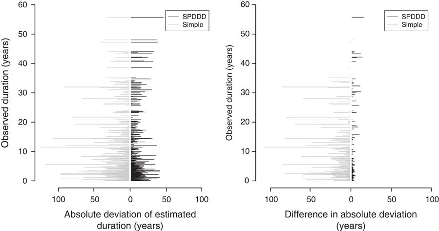
To demonstrate the better fit of our proposed model, we calculate the expected duration for uncensored peace and conflict spells according to our SPDDD model and the simple duration model. For our sample, the SPDDD model yielded predicted values closer to the observed values 60 percent of the time (330 out of 554 uncensored spells). Moreover, the deviation of prediction from the observed duration is much smaller for the SPDDD model than for the simple model. Figure 6 illustrates this point. In each panel, plotted to the left (in gray lines) are estimates from the simple model, whereas plotted to the right are estimates from the SPDDD model. The left panel shows the absolute deviation of predicted duration from the observed duration for all non-censored spells in our data set. The Y-axis shows the observed duration, and the X-axis shows the absolute difference between the observed and predicted duration from the two model. We can see that the simple model often yields deviation as large as 50 years, whereas the SPDDD model never yields deviation >50 years and seldom yields deviation as large as 25 years. The right panel of the figure illustrates the advantage of SPDDD model in terms of the difference in prediction error between the SPDDD model and the simple model. Lines to the left (in gray) show the absolute deviation (observed–predicted) from the simple model minus the absolute deviation from the SPDDD model for the cases where SPDDD performs better than the simple. Similarly, the lines to the right (in black) show the absolute deviation (observed–predicted) from the SPDDD model minus the absolute deviation from the simple model for the cases where the simple model performs better than the SPDDD model. We can see clearly that the SPDDD model performs better than the simple model most of the times and by a great extent.Footnote 25
In-sample prediction assessment Note: this figure compares model fit and in-sample prediction between simple Weibull model and the split-population duration-duration-duration (SPDDD) model. The left panel shows the absolute deviation of the predicted duration for the two models, whereas the right panel shows the difference in absolute deviation. In each panel, gray lines (plotted to the left) refer to Simple model whereas black lines (plotted to the right) refer to the SPDDD model.

CONCLUSION
This might be the end to this article, but it is hopefully the beginning of further research to theoretically and empirically embrace the notion that we need to treat pre-conflict peace duration, conflict duration, and post-conflict peace duration as interdependent processes. Our main argument is that we should account for the unobserved status of immunity from conflict as well as the unobserved factors that generate an interdependence between pre-conflict, conflict, and post-conflict processes.
Herein, we introduced an estimation approach that captures important elements of our theoretical argument. Our Monte Carlo simulations confirm that a failure to account for the unobserved immunity and/or interdependence leads to biased inferences. The empirical results also demonstrate that a model that corrects for these two inferential problems provides a better model fit. Our proposed model not only fits the data better but also reveals that some of the covariates that were thought to influence peace duration also influence the immunity from conflict. In fact, some estimates, especially the political exclusion of ethnic groups, become less precise in the peace duration equations once we account for the possible immunity of cases. Although ethnic exclusion consistently impacts on conflict duration (Wucherpfennig et al. Reference Wucherpfennig, Metternich, Cederman and Gleditsch2012) (even though in the SPDDD model less precise (p-value=0.13)), its effect is less certain in regard to pre- (p-value=0.24) or post-conflict peace duration (p-value=0.31). Similar observations can be made for GDP per capita. Of course, we are cautious about a final interpretation of these results as further research has to provide insights into whether the underlying assumption of the SP model that the immunity process is uncorrelated with the duration processes needs to be relaxed.
A further important insight of our work is that although peace and conflict durations seem to be related through unobserved factors, the main predictive improvement of our empirical model comes from modeling whether or not countries are immune from initial or further conflict. According to our theoretical argument, this would imply that once we account for whether actors are unsatisfied with the status quo, we can improve the actual duration modeling. In fact going back to our empirical model, there is evidence that once we model the immunity of cases, we also get more precise estimates for the interdependence between durations (θ p-value SUD=0.46; θ p-value SPDDD=0.13) and a decrease in the AIC score (SUD=9886; SPDDD=9868). This again highlights the importance of modeling the theoretically implied data-generating process as closely as possible. We believe that our empirical results support the case for further research focussing on both the interdependent nature of durations and the immunity of certain cases from conflict.