1 Introduction
Political science is making welcome progress out of what Morgan and Winship (Reference Morgan and Winship2014, 10–13) call the “Age of Regression”—the dark period between quasiexperiments and causal inference in which nearly every claim was tested with a linear model and concerns about confounders were addressed with the addition of yet another control variable. Today’s scholars have available to them a much wider array of statistical methods that conform far more closely to the logic of their theories. This is exceptionally good news for political science.
That said, there are still a handful of areas in which statistical inference is guided more by residual linear-additive thinking than by the logic of the problem at hand (Abbott Reference Abbott1988). Foremost among these are tests of asymmetric hypotheses—situations in which the hypothesized role of
 $X$
is to establish a limit on the variation of
 $Y$
(Lieberson Reference Lieberson1985, ch. 4). Examples of these hypotheses can be found in every subfield of political science. The literature on the democratic peace (Maoz and Russett Reference Maoz and Russett1993; Russett Reference Russett1994; Gartzke Reference Gartzke1998; Bueno de Mesquita et al.
Reference Bueno de Mesquita, Morrow, Siverson and Smith1999) is an obvious one: the presence of dyadic democracy places an upper limit on the hostility of interstate relations.Footnote
1
The distinguishing feature of these hypotheses is the conspicuous absence of observations from a region of the data space.
In this article, we provide a reevaluation of the methodology of asymmetric hypotheses. We argue that, because the absence of observations is the phenomenon of interest, data boundaries are more theoretically interesting than the central tendency of the data or a hypothesis of no effect. Therefore, we present a suite of tools useful for data exploration, rather than hypothesis testing. These tools allow one to discover boundaries that separate the region in which observations are present from the region in which observations are mostly or entirely absent and to gauge the uncertainty around those boundaries. One can use these tools to test hypotheses or to preprocess and explore data as a complement to further analysis and theory-refinement (Seawright Reference Seawright2016).
We should emphasize the fact that, although this is a methodological article, its main contribution is conceptual. The methods used to estimate boundaries, while helpful in that capacity, are most useful as concrete illustrations of a fruitful perspective on social phenomena, the asymmetric relationship, that cannot be fully conceived from within the confines of the linear model (or, for that matter, the average treatment effect). While the methods will certainly improve empirical research, our main hope is that widespread comprehension of asymmetric hypotheses will fuel more nuanced theorizing and motivate further methodological progress.
This article proceeds in five parts. In the next section, we motivate the discussion of asymmetric hypotheses. Following that, we evaluate the current state of the art for testing asymmetric hypotheses: multiplicative interaction terms and set-theoretic approaches. Third, we describe three lesser-known econometric techniques that incorporate the best features of these methods while avoiding their drawbacks. We then present three examples of how asymmetric hypotheses can be studied with this suite of tools. We conclude by discussing different techniques that can be used to estimate this boundary, and we illustrate their strengths and weaknesses in the context of three different asymmetric hypotheses.
1.1 Motivating the study of asymmetric hypotheses
The robust relationship between district magnitude and electoral system size is one of the most well-known and influential findings in all of social science. It is also an outstanding example of an asymmetric hypothesis. In Duverger (Reference Duverger1963)’s canonical presentation, the author argues that single-member district plurality (SMDP) electoral systems are sufficient to produce a two-party system—or equivalently, that a non-SMDP electoral system is necessary to produce a multiparty system.
The hallmark of asymmetric relationships is quite dramatic: cells of a table, or regions of a scatterplot, that are conspicuously devoid of observations. Importantly, when
 $X$
is continuous, asymmetric relationships typically produce a “floor” or a “ceiling” below or above which observations are rarely, if ever, found (Goertz, Hak, and Dul Reference Goertz, Hak and Dul2013). Noting the absence of observations in a scatterplot redirects the analyst’s attention toward an important feature of the data that often goes overlooked but is almost always of great theoretical interest: the boundary between zones of data and no-data.
A test of Duverger’s law: the relationship between district magnitude and the effective number of parties (Taagepera and Shugart Reference Taagepera and Shugart1993).

Like many before them, Taagepera and Shugart (Reference Taagepera and Shugart1993) and Li and Shugart (Reference Li and Shugart2016) test the empirical implications of this relationship. While Taagepera and Shugart (Reference Taagepera and Shugart1993) discover that, consistent with the original hypothesis, there is an upper limit on the effective number of seat-winning parties in districts of certain magnitude, Li and Shugart (Reference Li and Shugart2016) find that this upper limit is better predicted by alternative institutional variables. These results serve as an excellent motivating example because both studies are explicitly interested in estimating the upper limit of observations that can be seen in Figure 1. In other words, neither Duverger nor the authors is especially interested in the central tendency of the data or the residual distance between observations and the regression line. Rather, their focus is on the region of the data space—the ominous “Forbidden Zone” in Figure 1—in which, according to Duverger, few if any observations should be found. They seek to estimate the placement and characteristics of a line that describes the upper limit of the set of observed cases, rather than the central tendency of the data.
The ubiquity of these “Forbidden Zones” has motivated scholars to turn toward the study of “asymmetric” hypotheses (Clark, Gilligan, and Golder Reference Clark, Gilligan and Golder2006). An asymmetric relationship is one in which the primary theorized role of
 $X$
is not to increase or decrease the average value of
 $Y$
—though it may do so incidentally—but rather to establish a limit on its variation. It is the maximum (or minimum) value of
 $Y$
, rather than its average value, that varies as a function of
 $X$
. Returning to the Duverger example in Figure 1, the value of
 $X$
(district magnitude) has an impact on
 $Y$
(the effective number of seat-winning parties) not by changing its average value but rather by providing an upper limit to its variation: in large districts, there may be many parties or there may be few, but as district size decreases so too does the maximum number of effective seat-winning parties.
Exploring data boundaries has substantial implications for how asymmetric hypotheses are studied. While symmetric hypotheses lend themselves to estimating the central tendency (i.e., the conditional mean) of the data, asymmetric hypotheses are concerned with its limit. Put another way, investigating data boundaries is not reducible to merely comparing
 $E[Y|X=0]$
and
 $E[Y|X=1]$
(or
 $E[Y|X=n]$
) because these quantities say nothing about the largest or smallest possible value of
 $Y$
we can expect for given values of
 $X$
. For example, a theory about how, on average, an increase in district magnitude leads to an increase in party system size misses an enormously important fact about the world if the absence of such magnitude limits the formation of multiparty systems. If scholars focus on these latter sorts of relationships, then they will be able to leverage a rich and diverse set of tools to test their more nuanced theories in a principled way.
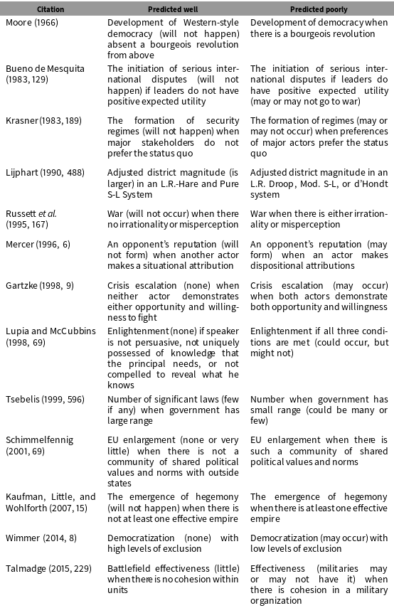
Examples of asymmetric hypotheses from the political science literature. Column 2 shows the range of input that predicts the outcome well, whereas column 3 describes the range that does not.

Asymmetric hypotheses, and the boundaries they produce, are of interest to virtually every subfield of political science. In Table 1, we provide several illustrative examples of prominent studies of asymmetric hypotheses across the discipline. In each case, we note when outcomes are either predicted well or predicted poorly. Our goal is to show that, regardless of one’s methodological persuasion, there is a common logic that underpins asymmetric hypotheses that all political scientists share. The exciting prospect of a renewed, unified focus on asymmetric hypotheses is that many scholars seem to think in these terms, and there are a variety of methods, quantitative and qualitative, for studying them.
In the next section, we review commonly used methods for studying asymmetric hypotheses. We first discuss the pros and cons of set-theoretic approaches. Then we show, in agreement with Clark, Gilligan, and Golder (Reference Clark, Gilligan and Golder2006), that there is nothing about large-N statistical techniques that precludes them from being used to study asymmetric hypotheses. However, we argue that multiplicative interaction terms are ill-suited to the task because they are designed to estimate the central tendency of the data rather than its upper or lower bound.
2 Asymmetric Hypotheses: The State of the Art
Two methodologies define the current state of the art when it comes to testing asymmetric hypotheses: Qualitative Comparative Analysis (QCA) and multiplicative interaction terms. Below, we outline each and highlight their strengths and weaknesses before moving on to a discussion of methods that combine the strongest points of each.
2.1 Set-theoretic approaches: Varieties of qualitative comparative analysis
Set-theoretic techniques, such as csQCA and fsQCA (Ragin Reference Ragin1987, Reference Ragin2000, Reference Ragin2008), have come under fire in recent issues of Political Analysis (Hug Reference Hug2013; Braumoeller Reference Braumoeller2015; Krogslund, Choi, and Poertner Reference Krogslund, Choi and Poertner2015). Yet their proponents should be lauded for their focus on the key quantity of interest in asymmetric hypotheses: boundaries between zones of data and no-data.
Set-theoretic approaches focus on the absence of data by modeling which of the logically possible combinations of qualitative conditions preclude certain outcomes, as opposed to quantitative techniques which measure the extent to which independent variables covary (Thiem, Baumgartner, and Bol Reference Thiem, Baumgartner and Bol2016). Even if two variables covary, that does not mean that in combination they are either necessary or sufficient for an outcome. This observation leads Ragin to argue that “
 $\ldots$
the variable-oriented strategy is incapacitated by complex, conjunctural causal arguments” (Ragin Reference Ragin1987, 69). In short, QCA advocates argue that asymmetric hypotheses can be best understood using set-theoretic methods rather than regression-based techniques.
While set-theoretic techniques have gained popularity since Ragin (Reference Ragin1987)’s early work, critics argue that the list of assumptions for QCA is long and quite restrictive and that the technique tends to produce unreliable results. Seawright (Reference Seawright2005) points out that QCA can only uncover relationships that are either additive linear or multiplicative linear. Hug (Reference Hug2013) shows that QCA can produce misleading inferences if measurement error is not taken into account. Even more problematic, critics have shown that QCA tends to produce false- positive results (Braumoeller Reference Braumoeller2015). Finally, Krogslund, Choi, and Poertner (Reference Krogslund, Choi and Poertner2015) cast further doubt on QCA by showing that a random variable added to a model can often be identified as a critical component of a causal relationship.
The main issue with fsQCA for our purposes is that the boundary of the data-free zone is imposed by the researcher and not empirically estimated. While researchers can calibrate the values of
 $X$
and
 $Y$
based on substantive knowledge of cases, the boundary between the data and the region in which few or no observations should be found is the line
 $Y=X$
. Yet, as far as we know, no asymmetric theory is specific enough to justify the a priori assumption that boundary lies at
 $Y=X$
(as opposed to, say,
 $Y=\frac{X}{2}$
or
 $Y=X^{2}$
). The boundary should be estimated rather than assumed. These issues and assumptions make set-theoretic techniques less than ideal for studying asymmetric hypotheses.
2.2 Interaction terms
In the quantitative tradition, Clark, Gilligan, and Golder (Reference Clark, Gilligan and Golder2006) (hereinafter, CGG) offer the most comprehensive description of asymmetric hypotheses and justification for why they are vital to social science. They claim that previous attempts to study asymmetry suffer from two different pathologies: the techniques either take a deterministic view of mechanisms in the social world (Ragin Reference Ragin1987, Reference Ragin2000; George and Bennett Reference George and Bennett2005), or require outcomes to be monocausal (Braumoeller and Goertz Reference Braumoeller and Goertz2000). CGG argue that a more appropriate technique for testing asymmetry would take into account the stochastic nature of the social world. They argue that the use of interaction terms in the standard linear model below is capable of capturing these effects:
 $$\begin{eqnarray}Y=\unicode[STIX]{x1D6FD}_{0}+\unicode[STIX]{x1D6FD}_{1}X_{1}+\unicode[STIX]{x1D6FD}_{2}X_{2}+\unicode[STIX]{x1D6FD}_{3}X_{1}X_{2}+\unicode[STIX]{x1D716}\end{eqnarray}$$
Although CGG correctly diagnosed the problem, there is a serious flaw in their proposed solution: it fails to model the appropriate attributes of the data.Footnote 2 What is being modeled in an OLS regression is the central tendency of the data—the average value of the dependent variable, conditional on covariates. What distinguishes asymmetric from symmetric hypotheses is the fact that the former produce distinct zones of data and no-data. Accordingly, the quantity of interest in the case of an asymmetric hypothesis is the upper or lower boundary of the data. As we demonstrate below, CGG’s own example of the determinants of party system size is better conceived of as a data-boundary question rather than a central-tendency question.
3 Having the best of both worlds
We have just argued that set-theoretic methods capture the concept of asymmetric hypotheses very well but are fraught with inferential peril, while multiplicative interaction terms model the central tendency of the data rather than their limits. For those reasons, we cannot recommend the use of either for evaluating asymmetric hypotheses.
Below, we describe three methods that combine the best features of these two techniques—a fundamental recognition that the boundary between the region in which data are present and the region in which they are nearly or entirely absent is the quantity of interest and the ability to estimate rather than assume that boundary.
3.1 Quantile regression
Goertz, Hak, and Dul (Reference Goertz, Hak and Dul2013) present quantile regression (QR) as a regression-based approach for modeling data thresholds with error. They suggest that asymmetric hypotheses require that analysts turn their attention away from conditional means and toward quantiles, which represent “ceilings” and “floors” delineating zones of data.
As the authors explain, “The key principle to note is that ceiling and floor hypotheses involve a fundamentally different orientation to hypotheses and data analysis: Ceiling and floor hypotheses are about drawing boundary lines between zones of data and zones of no-data; they are not about drawing lines through the middle of data” (Goertz, Hak, and Dul Reference Goertz, Hak and Dul2013, 20). Ceiling and floor hypotheses are typically asymmetric hypotheses: they imply that the range of possible observed values change with different values of independent variables (a rich state has a lower limit on its level of democracy, for example (Goertz, Hak, and Dul Reference Goertz, Hak and Dul2013, 20)).
QR works well for asymmetric hypotheses because it does not model the relationship between
 $X$
and the mean of
 $Y$
. Rather, it models the relationship between
 $X$
and some prespecified boundary on the value of
 $Y$
, often the 95th (upper boundary) or 5th (lower boundary) quantile. QR is also exceptionally robust to different distributions of data, a feature that allows it to produce reasonable estimates when other techniques fail.Footnote
3
In addition, the regression line for a particular quantile demonstrates an important point that CGG also discuss: the treatment of counterexamples. In substantive terms, a “ceiling” regression line through the .95 quantile means that 5 out of every 100 observations are treated as counterexamples, or cases which stand outside of the asymmetric hypothesis derived from the theory, a priori (Goertz, Hak, and Dul Reference Goertz, Hak and Dul2013, 29).
Thus, QR retains the intuition of CGG that it is necessary to model asymmetry with an understanding of the stochasticity of the social world. Yet, it is an improvement because QR explicitly focuses on estimating the object of interest for asymmetric hypotheses—data boundaries—and provides an improved approach to the question of error and counterexamples.
While QR shows that it is possible to use regression-based techniques to test asymmetric hypotheses, it is vulnerable to one criticism: while the threshold is estimated, the exact quantile to use to estimate it is assumed a priori rather than derived from the characteristics of the data. The scholar is given great latitude in determining what amount of error “seems right.” While Goertz, Hak, and Dul (Reference Goertz, Hak and Dul2013) provide a procedure for determining which quantile should be estimated (the Optimum Boundary Line), it is cumbersome, particularly once extended beyond bivariate settings, and cannot be directly compared across studies. It is telling that even after discussing the OBL technique, they admit that despite finding it useful for guiding which line should be used, “we eventually want to make some comparisons across studies. One way to do this is to take a fixed standard an obvious choice is the .95 quantile regression” (Goertz, Hak, and Dul Reference Goertz, Hak and Dul2013, 29). So, in practice, the analyst is often left to convention when deciding where to place the boundary.
3.2 Stochastic frontier analysis
Stochastic frontier analysis (SFA) is a modeling technique from the field of economics that is designed to estimate cost and production frontiers rather than expected values. The canonical example takes the form
 $y_{i}=f(X_{i};\hat{\unicode[STIX]{x1D6FD}},\unicode[STIX]{x1D709}_{i})$
, where
 $f$
is the production frontier,
 $X_{i}$
are the explanatory variables,
 $\hat{\unicode[STIX]{x1D6FD}}$
is the vector of parameters of the production function to be estimated, and
 $\unicode[STIX]{x1D709}_{i}$
, is a compound error term that adds to the normal, Gaussian error (
 $v_{i}$
) of the standard regression model a representation of inefficiency for each observation (
 $-u_{i}$
) (Aigner, Lovell, and Schmidt Reference Aigner, Knox Lovell and Schmidt1977; Meeusen and Van Den Broeck Reference Meeusen and Van Den Broeck1977). This error term allows SFA to take the burden of quantile or counterexample specification out of the analyst’s hand and put it into a familiar estimation routine that looks much like the standard linear model.
Most economists who use SFA take the production frontier to be in the Cobb–Douglas form, where the output of firms are a multiplicative function of land, labor, and capital. Although the Cobb–Douglas is illustrative because the frontier represents the theoretical maximum level of production for a firm, it is not ideal for most political science questions because, by definition, the absence of one of the factors of production leads to zero total production. The general SFA model is flexible enough to handle different specifications of
 $f$
, but the shape of the boundary is most often assumed to be linear (Simar and Zelenyuk Reference Simar and Zelenyuk2011, 3). Importantly, it models outcomes that look much like an asymmetric hypothesis with heteroskedastic data: firms can theoretically produce up to the frontier, so the zone above the frontier should contain few or no observations.
However, data boundaries are not absolute. Some observations are above or below frontiers due to inherent noise around the estimated boundary, or conceptual imprecision that results in measurement error. Herein lies another aspect of the value-added of SFA: while fuzzy-set techniques model conceptual imprecision, the handling of measurement error is left to the analyst; however, in SFA the routine estimates the location of the line and, by extension, how many observations are allowed to fall on the other side due to error that is familiar from other regression models. This corresponds to the first component of the compound error term in SFA models, commonly denoted as
 $v_{i}$
. In the canonical example, land, labor, and capital are the three inputs posited to produce output, but there is some inherent randomness around the frontier (i.e., “noise”), that corresponds to the familiar
 $\unicode[STIX]{x1D716}$
term from linear models.
In addition to the inherent stochasticity around the frontier, there is a second source of randomness that enters into the model. Even if a firm has an ideal mix of the three inputs, it could still underproduce due to inefficiency from exogenous shocks, bad luck, or any number of other factors (as well as overproduce for converse reasons). SFA is ideal for estimating data boundaries because its estimates include both a standard Gaussian error and a representation of how much or little a particular observation deviates from the production frontier. This leaves the final model to take the form of
 $Y_{i}=\unicode[STIX]{x1D6FD}_{0}+\unicode[STIX]{x1D6FD}^{^{\prime }}X_{i}+v_{i}-u_{i}$
(Greene Reference Greene, Fried, Knox, Shelton and Schmidt2008; Simar and Zelenyuk Reference Simar and Zelenyuk2011).
In this manner, SFA deals with the thorny question of counterexamples and the complex nature of the social world. Just as firms may outproduce what a production frontier would predict, states can also have greater levels of democracy than their level of GDP would indicate. Accordingly, SFA recovers the same insights that QCA does by using statistical inference rather than assumptions.
SFA is not without its own assumptions, of course. The main assumption of interest involves the compound error term. The distributional assumption of the error around the frontier,
 $v$
, is familiar, as it is assumed to follow a Gaussian distribution with zero mean. A variety of distributions could be used to model the second, nonpositive inefficiency error that accounts for the amount each observation fails to reach the frontier: typically,
 $u$
can be distributed half-Normal, exponential or gamma, depending on the data (Greene Reference Greene, Fried, Knox, Shelton and Schmidt2008). The variance of
 $u$
can also be modeled as a function of
 $X$
. While this flexibility is welcome, it is also limiting, in that inefficiency terms that do not conform to these distributions can produce irregular results. If the distribution of the errors is too left-skewed, for example, the procedure may not be able to successfully estimate the inefficiency.
In sum, SFA is preferable to fsQCA and interaction terms because it allows analysts to estimate threshold surfaces with a confidence interval that provides not only a measure of uncertainty around the exact location of the threshold but also around the estimate of the inefficiency of each observation relative to the boundary via the compound error term. However, SFA comes with costs as well. It requires rigid functional form assumptions for the boundary and the error terms, and it can be fragile if those assumptions are not met.
3.3 Nonparametric frontier models
Another option for estimating data boundaries are “nonparametric frontier models” (NFM) such as data envelopment analysis (DEA). These models also attempt to estimate a frontier from observed data, but because these models are nonparametric there are no rigid functional form assumptions. Unlike SFA, no parametric restrictions (linear or otherwise) are made about the distribution of inputs on the boundary. We discuss classical DEA prior to presenting more recent developments.
DEA is a procedure invented by Farrell (Reference Farrell1957) for use in operations research and organization science (Seiford Reference Seiford1996). It is primarily used to model productive efficiency of decision making units (e.g., the U.S. Post Office) when a production process involves a structure of multiple inputs and outputs (e.g., delivery of the daily mail). Here, the data boundary is the line which defines the maximum combination of outputs that can be produced for a given set of inputs. Observations that lie below the frontier reflect some degree of inefficiency in the production process.Footnote 4
Formally, the data boundary (
 $\unicode[STIX]{x1D6F9}$
) can be expressed as
 $$\begin{eqnarray}\unicode[STIX]{x1D6F9}=\{(x,y)\in \unicode[STIX]{x1D6F9}|(\unicode[STIX]{x1D6FE}^{-1}x,\unicode[STIX]{x1D6FE}y)\notin \unicode[STIX]{x1D6F9}\hspace{2.22198pt}\text{for any}\hspace{2.22198pt}\unicode[STIX]{x1D6FE}>1\},\end{eqnarray}$$
where
 $(x,y)$
is any ordered pair that falls on the boundary and
 $\unicode[STIX]{x1D6FE}$
is a constant. So, for any ordered pair on the boundary, as well as any constant
 $\unicode[STIX]{x1D6FE}>1$
, no other ordered pair that multiplies
 $x$
by
 $\unicode[STIX]{x1D6FE}^{-1}$
and
 $y$
by
 $\unicode[STIX]{x1D6FE}$
can also be on the boundary.
Nonparametric boundary estimation requires three minimal assumptions about the boundary. First, one assumes that inputs and outputs are freely disposable, which simply means that increasing inputs in isolation will not lead to a decrease in outputs. Further, any level of input that produces a given level of output can also produce less of it, respectively. Second, the “no free lunch” assumption states that production is impossible without the use of some positive inputs. Third, the boundary set
 $\unicode[STIX]{x1D6F9}$
is assumed to be convex, which follows from the convexity of preferences in economics. In other words, for any two bundles of an input and output that are each on the frontier, a weighted average of the two bundles is also on the frontier.Footnote
5
The original DEA estimator uses all three assumptions to envelop data without imposing a parametric structure on the distribution of
 $(X,Y)$
on
 $\unicode[STIX]{x1D6F9}$
. However, other estimators exist that do not require all three assumptions. The Free Disposal Hull (FDH) estimator, for example, extends DEA by maintaining the free disposability assumption while relaxing convexity (Deprins, Simar, and Tulkens Reference Deprins, Simar, Tulkens, Marchand, Pestieau and Tulkens1984). The convexity assumption requires the boundary to make predictions about all possible values of
 $X$
, not just those that are observed. When convexity is relaxed, predictions are only made about cases that are observed, leading to more persuasive estimates (Ray, Kumbhakar, and Dua Reference Ray, Kumbhakar and Dua2015). In FDH, the data boundary is estimated using the lowest “staircase” monotone curve covering all the data points. As a result of this “staircase” approach, FDH algorithms are easy to compute.
While DEA and FDH have the benefit of not assuming a particular functional form for the frontier (Simar and Wilson Reference Simar and Wilson2013), the assumption that all observations are attainable means that no noise is assumed in the data generating process. In other words, the distance between an observation and the frontier is due only to inefficiency, not measurement error, and no observations are permitted to fall outside of the frontier. In addition, DEA and FDH estimate frontiers that fluctuate widely if there are outliers or other extreme values in the data. Relatedly, these techniques do not estimate smooth boundaries. Rather, DEA and FDH produce boundaries with many nonsmooth points where “the estimated curve repeatedly stays flat and jumps, and the location of jumps [depends on particular
 $X$
values and] has no appropriate interpretation” (Noh Reference Noh2014, 503). Recently, DEA and FDH have been extended to remedy these discontinuities by accounting for measurement error, and these innovations provide a more flexible framework for the study of asymmetric hypotheses.
3.3.1 Accounting for measurement error
Recent innovations in NFMs allow one to retain the computational ease of DEA and FDH while simultaneously accounting for measurement error. While a fully nonparametric model with both noise and inefficiency is not identifiable (Hall and Simar Reference Hall and Simar2002, 523),Footnote 6 NFMs can be amended to account for unusual observations. The beauty of these extensions is that they are incredibly robust and widely prolific—one can choose no fewer than ten different modifications of data envelopment techniques.Footnote 7 These extensions outperform DEA and FDH in the presence of noise (Simar Reference Simar2007), and are less sensitive to extreme values in the data (Simar and Zelenyuk Reference Simar and Zelenyuk2011; Daouia, Florens, and Simar Reference Daouia, Florens and Simar2012).Footnote 8 In addition, each of these extensions has reasonable criteria for drawing boundaries that allow for measurement error: they build error into the techniques by considering all points within some bandwidth around the edge of the data to be drawn from a probability distribution. Finally, these techniques have a unique and robust way of dealing with inefficiency—they do not attempt to model it. Instead, NFMs estimate the density of the observations most relevant to the boundary, ignore the inefficiencies of individual observations in the estimation process, and only compute relative efficiencies after the boundary is drawn. In doing so, they combine the strengths of data envelopment with an estimation technique that allows for stochasticity around the boundary.
In the interest of space, we describe the most flexible option, kernel estimation (Noh Reference Noh2014; Daouia, Noh, and Park Reference Daouia, Noh and Park2016).Footnote 9 Kernel estimation produces a smooth frontier that envelops all the data and minimizes the area under the frontier curve (Noh Reference Noh2014). Unlike DEA and FDH, this smoothed frontier resists distortion by extreme observations because each observation is weighted by its estimated effect on the underlying boundary. However, because it is a smoothing technique, kernel estimation requires the selection of an appropriate bandwidth. Bandwidth selection is informative because bandwidth and curve complexity are inversely related. Therefore, the analyst can use the selection process to learn about the complexity of the underlying frontier, as well as let the data inform the complexity of the estimated curve. Noh (Reference Noh2014, 507–510) implements a bandwidth selection technique based on the Bayesian Information Criterion, shows that the criterion works well, and demonstrates the superiority of kernel estimation in simulation studies.
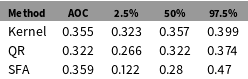
AOC estimates for the simulated data example.

3.3.2 But Can’t You Always Draw Boundaries?
A skeptic may wonder whether the boundaries estimated above are trivial.Footnote 10 All data have upper and lower boundaries, so there is no obvious distinction between symmetric and asymmetric hypotheses in that regard. There is, however, a meaningful distinction to be had based on the extent to which a hypothesized boundary precludes observations: data consistent with an asymmetric hypothesis should be rare or nonexistent in either the upper-left or the lower-right quadrant of a standard scatterplot. In other words, an upper or lower boundary will always exist, but that boundary is trivial if it does not preclude observations across a significant range of the data space.
Accordingly, we introduce a new criterion—Area Outside of the Curve (AOC)—to distinguish boundaries that are meaningful from those that are trivial. AOC is the ratio of the area outside of the estimated boundary (above for lower-triangular relationships, below for upper-triangular ones) to the total area of the scatterplot, defined as
 $(\max (x)-\min (x))\times (\max (y)-\min (y))$
. We calculate AOC for each technique using the simulated data example in Table 2, as well as report the 95% bootstrapped confidence intervals (5000 replicates). For the simulated asymmetric data, nearly half of the area is devoid of observations, regardless of the technique used. In practice, we expect AOC to be much smaller. This test is not meant to be overly restrictive. Rather, it is meant to weed out relationships that are not especially asymmetric. There is no obvious cutoff value between asymmetric and symmetric relationships, so based on our own simulations we propose what we hope is a fair test: to be considered a nontrivially asymmetric relationship, the AOC should be greater than or equal to 0.2 with 95% certainty, based on the estimated confidence intervals.
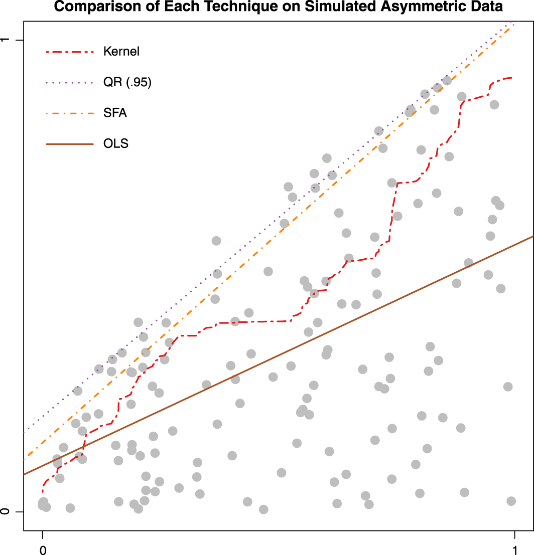
We estimate SFA, QR, and kernel estimation on simulated data. We include OLS to demonstrate that estimating the central tendency of data does not estimate its boundary.

In this section we have provided three different options for estimating data boundaries in asymmetric hypotheses. The techniques share two common tasks. First, the analyst must estimate with some degree of uncertainty the location of a single, fixed frontier. Second, the distance from a given observation (
 $X_{i},Y_{i}$
) to the frontier (in any direction) is unknown, and thus must be estimated. SFA and QR draw stochastic boundaries yet require specifying a particular functional form. The added benefit of accounting for noise around the boundary comes with the cost of either restricting the distribution of the errors and inputs (SFA) or specifying the quantile through which the boundary is drawn (QR). NFMs provide an alternative approach, ranging from the most canonical (DEA and FDH) to more flexible techniques (kernel smoothing). Within the data envelopment framework, this flexibility comes at the cost of potential sensitivity to extreme data as well as leaving inefficiency unmodeled.Footnote
11
Figure 2 shows how each technique performs on simulated asymmetric data. We include OLS as a point of comparison to reinforce the point that regression with an interaction term does not model the boundary of the data. While each technique is capable of estimating data boundaries, they are not equally suitable in all scenarios. Kernel estimation is well suited to applications with small samples because it is less sensitive to outliers. SFA works best when one has more data, is willing to subscribe to distributional assumptions, and is particularly interested in estimating the inefficiency of individual observations. Finally, QR is especially useful for comparisons across space or time because it is less sensitive than other techniques to substantial outliers that can make comparisons difficult. While the estimation is not limited by sample size, one must trade off the requirement to specify the quantile ex ante. In the next section, we apply each technique to an example for which it is suited.
4 Examples
We now turn to applications of our three techniques for evaluating asymmetric hypotheses—QR, SFA , and kernel estimation—to three examples of asymmetric hypotheses in the existing literature.Footnote 12 We show how asymmetric hypotheses can be investigated in three different scenarios. In addition to estimating the boundary, we include 95% confidence intervals around the boundary based on 5,000 bootstrap replicates. These bounds allow us to show how uncertainty varies with technique and sample size.
4.1 The domestic sources of transnational security cooperation
Koenig-Archibugi (Reference Koenig-Archibugi2004)’s investigation of the relationship between domestic political preferences and transnational security cooperation in the European Union offers a good example of an asymmetric hypothesis that would typically receive attention from qualitative scholars due to its small sample size. It also allows us to demonstrate the utility of kernel estimation in estimating the frontier of upper-triangular relationships. We chose kernel estimation for this example because it works well in small samples, despite being nonparametric, and as such it is the least sensitive to extreme observations.
In addressing the puzzle of why states would surrender political sovereignty by coordinating their foreign and security policy with other EU member states, Koenig-Archibugi argues that “attitudes toward supranational integration are shaped by distinct conceptions of sovereignty and political authority that prevail in the political culture of the member-states” (Koenig-Archibugi Reference Koenig-Archibugi2004, 167). Accordingly, he finds that these attitudes are shaped by a combination of material variables (such as political and economic power and regional governance institutions), as well as ideational variables (including measure of popular and elite-level European identity and policy conformity with other European states).
To investigate the domestic political sources of support for supranationalism, Koenig-Archibugi employs fsQCA and discovers the following asymmetric relationship: the combination of strong regional governance (based on the degree of constitutional federalism, the presence of special territorial autonomy, the role of regions in central government, and the existence of regional elections) and policy conformity (having preferences on specific policy issues that are consistent with the preferences of most other EU member states) are sufficient to generate national support for the European Union’s Common Foreign and Security Policy (CFSP).
In discussing the substantive implications of this relationship, the author argues that
a pluricentric constitutional culture removes an important conceptual obstacle—the idea of national sovereignty as unitary and indivisible—from the transfer of decisional powers to the European level. The anticipation that most decisions made in supranational fora would correspond to the government’s substantive policy preferences adds to this permissive factor a positive incentive to support supranationalization, and it is the combination of permissive and positive conditions that makes this particular conjuncture sufficient for the outcome (Koenig-Archibugi Reference Koenig-Archibugi2004, 164).
The author limits his investigation to the original thirteen members states of the European Union. This limited universe of cases makes fsQCA an ideal candidate for examining the possible combinations of conditions that produce supranational security cooperation.
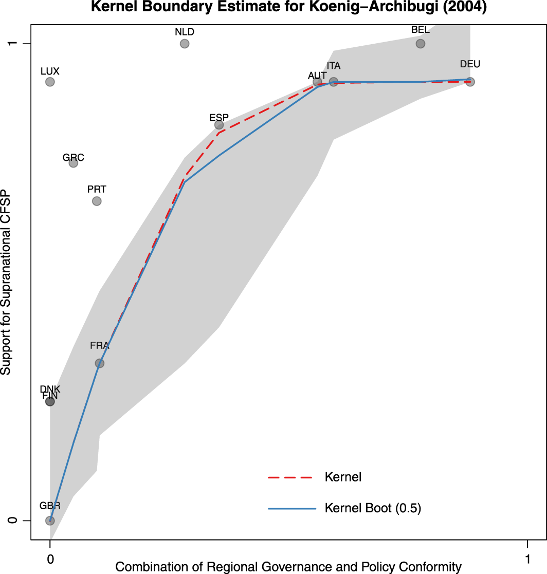
Replication of Koenig-Archibugi (Reference Koenig-Archibugi2004) using kernel estimation. The uncertainty around the boundary was generated with 5000 bootstrap replicates.

Figure 3 is a replication of Koenig-Archibugi’s findings, including a boundary line derived from kernel estimation and bootstrapped confidence intervals. The x-axis reflects fuzzy-set membership scores for EU member states along the intersection of regional governance and policy conformity (two of the six conditions coded in Figure 2 of the original article). The y-axis measures percent support for the EU’s Common Foreign and Security Policy (CFSP). The upper-triangular distribution of the data reflects a sufficiency plot, because each membership in the fuzzy set of supranationalist governments (y-axis) is at least as high as a state’s membership in the intersection of regional governance and policy conformity (x-axis) (Koenig-Archibugi Reference Koenig-Archibugi2004, 162–163).
We evaluate this asymmetric hypothesis using kernel estimation for three reasons. First, the OLS residuals from SFA models often violate the distributional assumptions of the inefficiency term, and this leads to unreliable inferences even when models are properly specified (Almanidis and Sickles Reference Almanidis and Sickles2011, 204). Second, we do not use QR because the .95 QR would be drawn through only two observations. This coarseness would throw away informative features of the data that a nonparametric technique can expose. Finally, we choose kernel estimation over other nonparametric techniques because it is the least sensitive to extreme observations.
After proceeding, we conduct an AOC test to verify the nontrivialness of this boundary. This exercise may not be necessary because the original analysis was done using fsQCA. Therefore, all observations must fall above the
 $Y=X$
line by construction. However, we conduct an AOC test as construct validity for our measure. As one can see in Table 3, the area outside the kernel boundary is quite large, indicating a strong asymmetric relationship. Despite the small sample size, the area outside the curve does not drop below 0.475 in the bootstrap replications.
AOC estimate for Koenig-Archibugi (2004), with 95% bootstrapped confidence intervals (1000 replicates).

We report the kernel estimation boundary in Figure 3. As one can see, the kernel boundary implies a diminishing effect of regional governance and policy conformity on support for supranational foreign and security policy. Even though the kernel estimation boundary is curved, its substantive interpretation remains unchanged from the original analysis—both the United Kingdom (lower left) and Germany (upper right) exhibit ideal-typical relationships between regional governance and policy conformity, and support for transnational security cooperation. Yet, our approach adds considerable value by showing the nonlinear relationship between regional governance, policy conformity, and the lower boundary on support for a supranationalist CFSP. This result can drive future work on what makes Spain, Austria, and Italy important cases for driving transnational security cooperation in the EU.
However, the bootstrapped confidence intervals show the potential dangers of using a statistical technique on an application with so few observations. Because we resample from 13 observations (5000 replicates), the variance in the boundary estimates is quite large. However, the median bootstrap, reported in blue, corresponds well to the original boundary. Despite wide variance at the margin, this similarity indicates that the boundary estimates are rather stable, even when resampling from such a small universe of cases. In general, this demonstration shows that kernel estimation provides a flexible technique for estimating asymmetric boundaries in studies with small samples.
4.2 Exploring the health–wealth nexus
Our second example of an asymmetric hypothesis comes from the voluminous literature on the relationship between economic status and health outcomes. This example shows the efficacy of QR for evaluating asymmetric hypotheses with many observations over time. In comparison, nonparametric techniques are less suitable for boundary analysis over time because sensitivity to outliers makes boundaries difficult to compare. We first demonstrate when wealth and health outcomes are asymmetrically related, prior to showing how this relationship changes over time. We conclude by reflecting on the substantive reasons why these patterns emerge.
Following Bergh and Nilsson (Reference Bergh and Nilsson2010), we test the claim that GDP per capita (purchasing power parity-adjusted) provides an upper limit on life expectancy. Our data cover the period from 1800–2015, so we are able to extend previous analyses by seeing the degree to which the upper boundary evolves.Footnote 13 Once we establish that this is a proper asymmetric relationship, we will be able to see how the region of low-GDP/high-life expectancy changes over time.
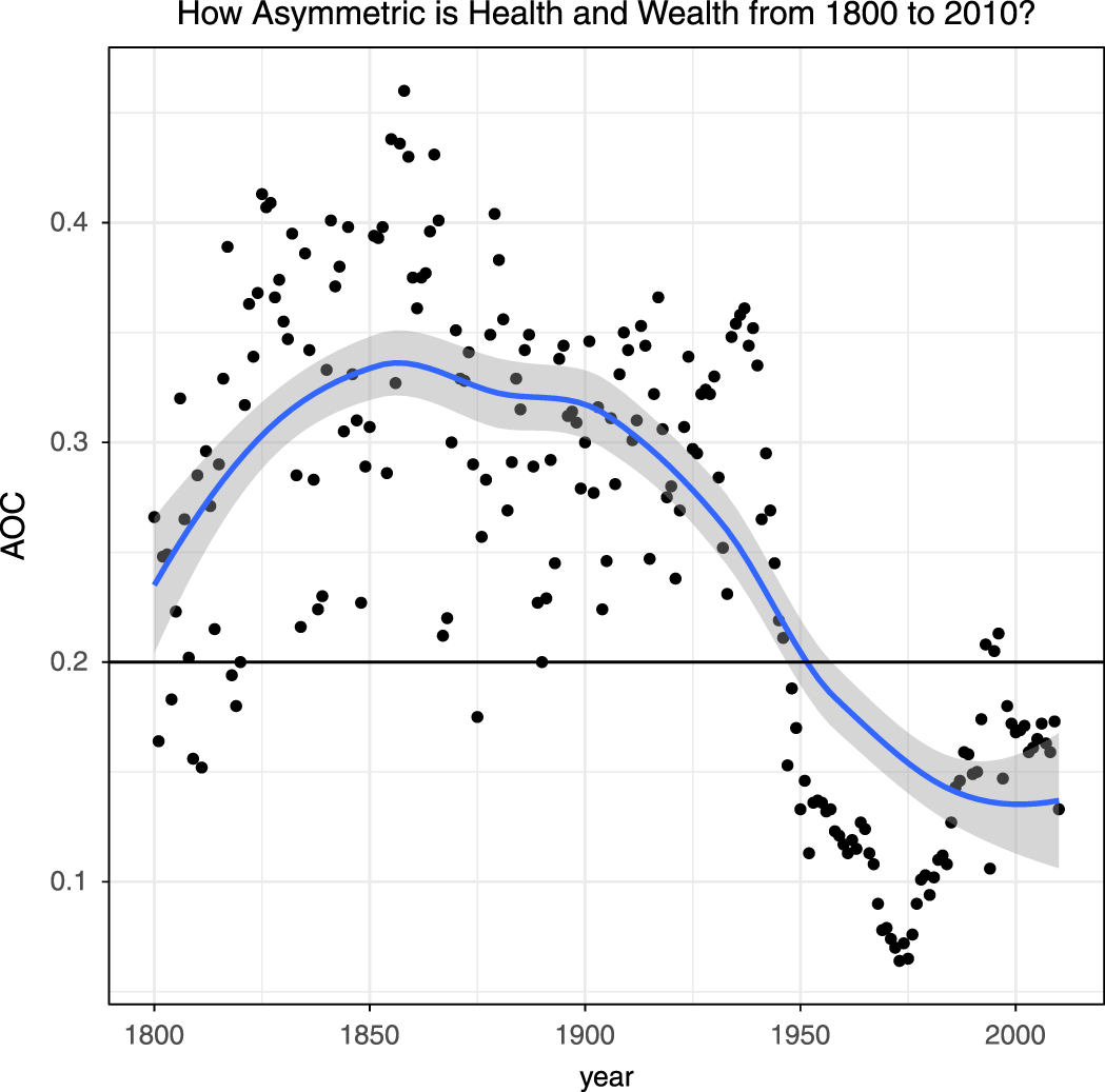
How AOC for the health–wealth example changes over time.

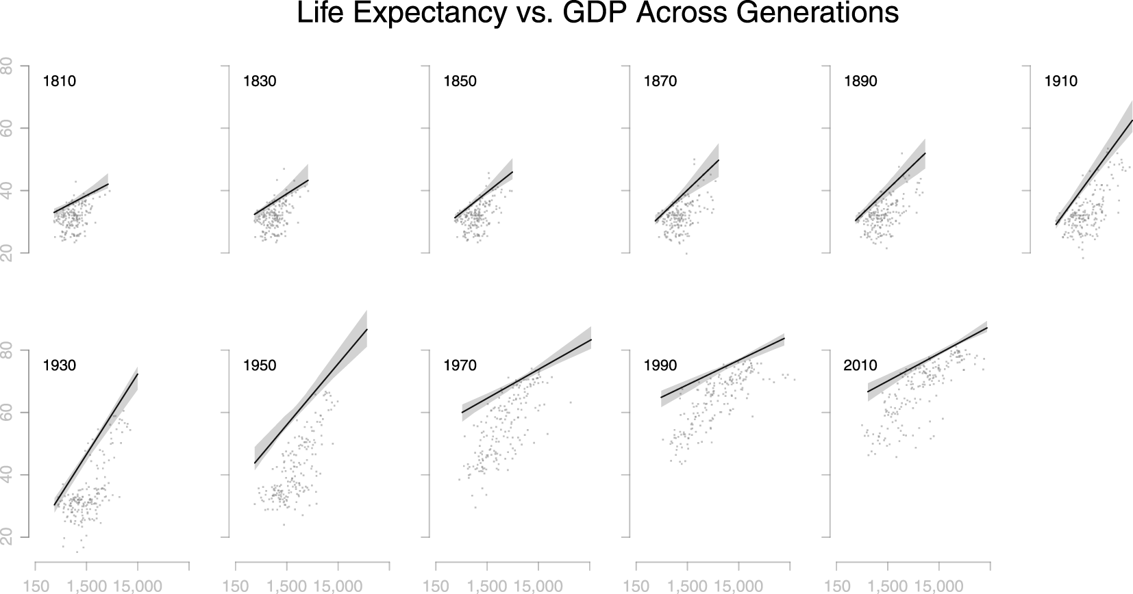
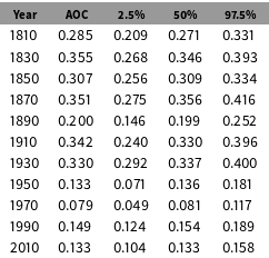
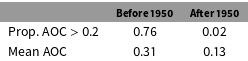
We re-estimate the QR model through the .95 quantile for each twentieth year from 1800 to 2015 and plot the resulting frontiers in Figure 5. We then use AOC to see if this relationship is asymmetric. This task is less straightforward when one analyzes time series data because an asymmetric hypothesis in one period may become symmetric in another. In Table 4, we report the AOC for each time period, as well as its 95% bootstrap confidence intervals. In periods prior to 1950, the relationship between health and wealth can be characterized as an asymmetric hypothesis because the AOC is typically above 0.2. However, after 1950, the relationship becomes more symmetric. This evolution becomes starker in Figure 4 and Table 5, where one can see the dramatic differences between years prior to and after 1950.
Wealth and the limits of human longevity.

AOC estimate for the Health–Wealth analysis over time, with 95% bootstrapped confidence intervals (1000 replicates).

The proportion of years in which the AOC is above the 0.2 threshold. Prior to 1950, the health–wealth relationship was almost always asymmetric. Since 1950 the relationship is much less asymmetric.

The QR boundaries are presented in Figure 5. We can see that, predictably, the upper limit that GDP places on life expectancy has risen dramatically over the last two centuries. In particular, the increase in life expectancy from 1920 to 1980 was spectacular, mostly due to advances in medicine and public health.
When viewed over time, the slopes of the boundaries are also substantively interesting. When the slope is flat, the upper boundary on life expectancy is more or less the same at all levels of GDP, but a steep line indicates that a state’s level of GDP has a pronounced limiting effect on the life expectancy of its citizens. Early in the 19th century, the slopes of the boundaries were much flatter than they became from mid-century on, and only recently have they gotten less steep. Roughly speaking, innovations in health care began to have a noticeable effect as early as 1890 in the richest countries, but it was not until about 1950 that the benefits of those innovations began to improve life expectancy in the poorest countries. In 1930, the upper limit of life expectancy in rich countries like the United States and Germany was about 60 years. By contrast, the upper limit of life expectancy in poorer countries like China and India was about 30 years. By the mid-1990s, however, China had achieved life expectancy nearly on a par with the United States (around 73 years).
In some cases, liberated colonies inherited elements of colonial healthcare systems. In our data, Uganda and Tanzania fit into the category of former colonial states where life expectancy outpaces development. In others, however, healthcare innovations diffuse and are adapted by large, developing states. This is most evident in China, where life expectancy surged between 1950 and 1970 (despite the murderous Great Leap Forward in the early 1960s). While both sets of cases provide examples of life expectancy outpacing economic development, the explanation behind this relationship operates via different causal mechanisms.
In addition, these factors help explain why the relationship between GDP and life expectancy became less asymmetric over time. Prior to the innovations and development of the mid-20th century, it is clear that in the absence of economic development, life expectancy was low. In other words, rather than predict life expectancy, GDP placed an upper limit on it. This relationship is the definition of an asymmetric hypothesis. However, since the 1950s, it is clear from looking at AOC and Figure 5 that the relationship has become more symmetric. This change suggests that the barriers to longevity in the poorest countries had been successfully pushed back, though substantial variation among poorer countries remains.
4.3 Party size, electoral systems, and democracy
Finally, we reexamine the findings on party system size that were presented by Clark, Gilligan, and Golder (Reference Clark, Gilligan and Golder2006). CGG explore the hypothesis that the number of parties in a given country (party system size) is a function of the interaction of electoral system permissiveness and social heterogeneity. Theoretically, these two dimensions limit the maximum number of parties, producing a frontier that is of great importance to scholars of comparative electoral systems. In Duverger’s (Reference Duverger1963) canonical presentation, the author argues that SMDP electoral systems are sufficient to produce a two-party system—or equivalently, that a non-SMDP electoral system is necessary to produce a multiparty system. Neto and Cox (Reference Neto and Cox1997) give these hypotheses more specific form by observing that “[t]he effective number of parties in a polity should be a multiplicative rather than an additive function of the permissiveness of the electoral system and the heterogeneity of the society.” CGG examine a simplified version of Neto and Cox’s model in order to demonstrate that much of the heterogeneity in party system size can be explained by social (in this case, ethnic) heterogeneity.Footnote 14 However, the authors’ interactive model fails to capture the intuition that, when the absence of data is the phenomenon of interest, our goal should be to delineate the boundary at which this absence begins. Interaction terms are incapable of doing this because OLS estimates the central tendency of the data.
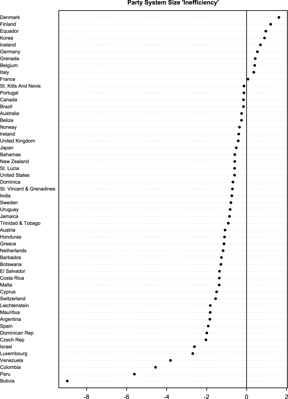
In this example, we show how SFA can be used to estimate the upper boundary of the data. Our stochastic frontier model retains the interactive essence of the CGG model, while estimating the stochastic upper bound of the data rather than their central tendency. SFA also allows us to model heterogeneity by making the magnitude of the inefficiency term a function of the same variables that define the frontier. The results in Figures 6 and 7 demonstrate how party system size can be understood as a boundary phenomenon rather than a matter of central tendency. The stochastic party system size frontier is described by a surface of the form:
 $$\begin{eqnarray}\displaystyle \mathit{Frontier} & = & \displaystyle 2.997-0.330\times \text{Electoral System Permissiveness}-1.056\times \text{Social Heterogeneity}\nonumber\\ \displaystyle & & \displaystyle +\,1.347\times \text{Electoral System Permissiveness}\times \text{Social Heterogeneity}.\nonumber\end{eqnarray}$$
This frontier describes the maximum size of party systems we should expect for given levels of electoral system permissiveness and social heterogeneity. In addition, the AOC for upper percentile of the frontier is 0.20, suggesting that this hypothesis is asymmetric (see Table 6).
One ought to note that, unlike other regression models, in SFA “parameter estimates by themselves have little informational value; they are simply means to the end of producing a frontier” (Fenn et al. Reference Fenn, Vencappa, Diacon, Klumpes and O’Brien2008, 94). This feature of SFA reinforces our point that studying asymmetric hypotheses does not reduce to null hypothesis significance testing. The frontier gives specific estimates for how the upper boundary of party system size is associated with various levels of electoral system permissiveness and social heterogeneity. The frontier also indicates how individual cases perform relative to their theoretical upper limit.
A reanalysis of Clark, Gilligan, and Golder (Reference Clark, Gilligan and Golder2006) using stochastic frontier analysis, showing the upper limit of party system size given social heterogeneity and electoral system permissiveness.

Inefficiencies in party system size.

AOC estimate for CGG (2006), with 95% bootstrapped confidence intervals (1000 replicates).

For this reason, scholars most often use SFA results to describe the “inefficiency” of individual cases—that is, how far the value of the dependent variable in a given case falls below the theoretical maximum dictated by the values of the independent variables. Substantively, these results show that some polities (Figure 7) are notably more “inefficient” than others at producing the expected number of parties given their electoral system and degree of social heterogeneity. Consider the case of Bolivia, the least “efficient” observation in the sample. Factors such as indigenous politics, labor dynamics within the tin and copper mining community, or political divisions between voters in the Andes versus populations in the Amazon basin may promote sui generis party dynamics which are otherwise nonideal from a theoretical point of view (Whitehead Reference Whitehead1981). Similar inefficiencies may exist in Colombia, where coffee, gold, and coca cultivation affect regional party formation, mostly through effects on local conflict dynamics (Richani Reference Richani2013).
Our reanalysis of CGG follows the lead of the set theorists in finding the boundary between the region in which observations occur and the region in which they largely do not (Figure 6). SFA also allows us to harness the statistical rigor of large-N models. In so doing data boundaries tell us something fundamentally different about the social world than regression models that estimate conditional averages. We can now usefully discuss the upper limit of party system size given electoral system size and social heterogeneity, as well as the performance of individual countries. Our results are indicative of how SFA can be used to explore data boundaries as well as how it can improve and respect the approaches of both set-theoretic and statistical methodologists.
5 Conclusion
This article presents both a conceptual clarification of asymmetric hypotheses and a discussion of the methodologies available to explore them. Most existing methods used by political scientists fail to capture the core insight motivating asymmetric hypotheses: the boundaries separating zones of data from areas that lack observations are the primary features of interest. While multiplicative interactive terms are incapable of modeling these boundaries, set-theoretic methods end up assuming a fixed boundary by construction. QR, SFA, and NFMs, by contrast, allow us to estimate the boundary as well as to explore the distance between the boundary and specific observations of interests. These techniques neither ensure nor preclude causal relationships. Instead, they equip the analyst to explore asymmetric hypotheses—a feature of the data that may previously have been overlooked.
We also hope to have shown that qualitative and quantitative approaches to asymmetric hypotheses can usefully inform one another and provided a set of methodological tools that will be useful to both. In so doing, we hope to have narrowed the schism between qualitative and quantitative scholars and opened the door for more question-driven rather than method-driven research.Footnote 15 Such an effort will facilitate continued progress away from the dogmatic “Age of Regression” and toward a future in which scholars test their theories with methods that conform to theoretical logic rather than continuing to shoehorn a complex social world into a linear-additive straitjacket.