







1. Introduction
A drop impacting a dry solid substrate will either spread tangentially to the surface without breaking or will splash, disintegrating into tiny droplets ejected radially outwards at velocities far larger than the impacting one (Yarin Reference Yarin2006; Josserand & Thoroddsen Reference Josserand and Thoroddsen2016). It is now known that the conditions under which splashing occurs does not only depend on the liquid properties, on the impact velocity and on the drop radius, as expressed by the well-known correlation proposed in Mundo, Sommerfeld & Tropea (Reference Mundo, Sommerfeld and Tropea1995), but also on other parameters such as the surrounding gas pressure (Xu, Zhang & Nagel Reference Xu, Zhang and Nagel2005; Riboux & Gordillo Reference Riboux and Gordillo2014; Stevens Reference Stevens2014; Gordillo & Riboux Reference Gordillo and Riboux2019), the roughness (Stow, Hadfield & Ziman Reference Stow, Hadfield and Ziman1981; Range & Feuillebois Reference Range and Feuillebois1998; Xu, Barcos & Nagel Reference Xu, Barcos and Nagel2007; Latka et al. Reference Latka, Strandburg-Peshkin, Driscoll, Stevens and Nagel2012; Quetzeri-Santiago, Castrejón-Pita & Castrejón-Pita Reference Quetzeri-Santiago, Castrejón-Pita and Castrejón-Pita2019a) or the substrate wettability (de Goede et al. Reference de Goede, Laan, de Bruin and Bonn2018; Quetzeri-Santiago et al. Reference Quetzeri-Santiago, Yokoi, Castrejón-Pita and Castrejón-Pita2019b; Quintero, Riboux & Gordillo Reference Quintero, Riboux and Gordillo2019), with wetting and roughness intimately related with each other, see e.g. Quéré (Reference Quéré2008).
It is the purpose of this contribution to analyse the spreading and splashing of droplets of low viscosity liquids such as water and ethanol or mixtures of both impacting at normal atmospheric conditions over rough substrates. These are, precisely, the most common conditions involving the impact of a drop against a solid found in both practical applications and in our daily life experience: indeed think, for instance, of rain drops falling on the sidewalk, which clearly is a rough substrate like the vast majority of solids. Our study will be limited to analysing those cases in which the surface is initially dry, a situation which differs from the similar – albeit simpler case because neither the topography of the substrate nor wetting effects are present – in which the drop falls on a pool or thin liquid film (Josserand & Zaleski Reference Josserand and Zaleski2003; Cimpeanu & Moore Reference Cimpeanu and Moore2018). It will also be assumed that the drop falls over the solid perpendicularly because the effects associated with the impact direction (Bird, Tsai & Stone Reference Bird, Tsai and Stone2009; Almohammadi & Amirfazli Reference Almohammadi and Amirfazli2017; Hao & Green Reference Hao and Green2017; Hao et al. Reference Hao, Lu, Lee, Wu, Hu and Floryan2019) can be easily accounted for using the framework put forward in, for instance, Gordillo & Riboux (Reference Gordillo and Riboux2019) and García-Geijo, Riboux & Gordillo (Reference García-Geijo, Riboux and Gordillo2020).
As it was mentioned above, Mundo et al. (Reference Mundo, Sommerfeld and Tropea1995) studied the case of drops impacting at normal atmospheric conditions on either smooth or rough dry surfaces and characterized the spreading–splashing transition through the so-called  $K$ parameter, or splashing parameter, which is nothing but a correlation involving the Reynolds and Ohnesorge numbers based on the liquid properties. Nevertheless, the experiments conducted by Xu et al. (Reference Xu, Zhang and Nagel2005) and Stevens (Reference Stevens2014) revealed that drop splashing can be suppressed by reducing the air pressure and also that the splash threshold velocity behaves non-monotonically for low values of atmospheric pressure, these facts indicating that drop splashing heavily depends on the properties of the surrounding gaseous atmosphere. The correlation found by Mundo et al. (Reference Mundo, Sommerfeld and Tropea1995), as well as the experimental results found by Xu et al. (Reference Xu, Zhang and Nagel2005) and Stevens (Reference Stevens2014), were reconciled by the theory presented in Riboux & Gordillo (Reference Riboux and Gordillo2014) and Gordillo & Riboux (Reference Gordillo and Riboux2019), where it is shown that the splashing of drops is produced by the lift force exerted by the air on the edge of the lamella. The ideas in Riboux & Gordillo (Reference Riboux and Gordillo2014) were developed for the case of smooth dry substrates, and it will be one of the purposes in this contribution to check whether they can also be applied to the case of rough solids or not.
In their now classical contribution, Stow et al. (Reference Stow, Hadfield and Ziman1981) analysed the splashing of drops on rough substrates, observing that the critical velocity for splashing decreases with increasing values of the amplitude of the roughness. Stow et al. (Reference Stow, Hadfield and Ziman1981) also proposed a correlation based on the Reynolds  $(Re)$ and Weber
 $(We)$ numbers and on the surface roughness in order to fit their experimental data and, later on, the experiments reported in Rioboo, Tropea & Marengo (Reference Rioboo, Tropea and Marengo2001) and Range & Feuillebois (Reference Range and Feuillebois1998) confirmed the observations in Stow et al. (Reference Stow, Hadfield and Ziman1981) that the critical Weber number for splashing depends on the amplitude of the substrate roughness. More recently, Roisman, Lembach & Tropea (Reference Roisman, Lembach and Tropea2015) proposed a correlation expressing that the critical Weber number for splashing does not depend on the roughness amplitude but on the slope of the substrate corrugations. In the same vein, but for the case of microstructured surfaces, Xu (Reference Xu2007), Tsai et al. (Reference Tsai, van der Veen, van de Raa and Lohse2010), Lembach et al. (Reference Lembach, Tan, Roisman, Gambaryan-Roisman, Zhang, Tropea and Yarin2010), Kim et al. (Reference Kim, Park, Lee, Kim, Hwan Kim and Kim2014), de Jong, Enríquez & van der Meer (Reference de Jong, Enríquez and van der Meer2015) and Yarin, Roisman & Tropea (Reference Yarin, Roisman and Tropea2017) showed that the transition from spreading to splashing depends on the geometrical arrangement of the micropillars. The influence of both air pressure and surface roughness on drop splashing was analysed experimentally by Xu et al. (Reference Xu, Barcos and Nagel2007) and Latka et al. (Reference Latka, Strandburg-Peshkin, Driscoll, Stevens and Nagel2012), who found that both aerodynamic forces and the substrate roughness play a role in the splashing of drop, but they did not provide with any type of fit, correlation or theory to quantify their observations. In addition, Josserand et al. (Reference Josserand, Lemoyne, Troeger and Zaleski2005) simulated the effect on drop splashing of a single obstacle placed on an otherwise dry and smooth substrate and compared the numerical results with experimental observations.
The previous revision reveals that there is a lack of physical understanding of the role played by the surface corrugations in triggering the splash, even at normal atmospheric conditions. Then, based on our own experimental observations, here, we present simplified models which, retaining the underlaying physics, provide with predictions for the splash threshold velocity at normal atmospheric conditions, in good agreement with observations. In addition, it will be shown that the equations describing the spreading of drops deduced in Gordillo, Riboux & Quintero (Reference Gordillo, Riboux and Quintero2019) can also be used to predict the observations with rough substrates. While Rioboo et al. (Reference Rioboo, Tropea and Marengo2001), Xu et al. (Reference Xu, Barcos and Nagel2007), Latka et al. (Reference Latka, Strandburg-Peshkin, Driscoll, Stevens and Nagel2012) and Hao (Reference Hao2017) establish a difference between two types of splashing namely, prompt splashing and corona splashing, here, we will make no distinction between them and will simply determine the conditions for which the drops keep their integrity after the impact (spreading) or they break into smaller and faster droplets (splashing). Let us point out here that this study focuses on the most common case of applications in which neither the spatial distribution nor the geometry of the protuberances of the rough substrate are controlled using microfabrication techniques.
The paper is structured as follows: in § 2 we describe the set-up and present the experimental results, § 3 is devoted to providing the theoretical models for the spreading and the splashing of drops and to showing comparisons of the predictions with the experimental observations. The main conclusions are presented in § 4.
2. Experimental set-up and phenomenology
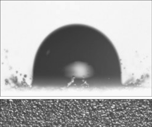
Figure 1 is a sketch of the experimental set-up used to produce water or ethanol drops of radii  $R$ impacting over different types of sandpapers, these being replaced after each measurement. The drops produced in this way fall with a variable and controllable velocity
 $V$ within the range of values indicated in table 1. The side and top views of the drop impact process are extracted from the analysis of the videos recorded using two different high-speed cameras: figure 1 shows that a Phantom V710, operated at 33 000 f.p.s. (frames per second) is used to get the images from above with a spatial resolution of 42
 $\mathrm {\mu }$m per pixel, whereas a Phantom V7.3, operated between 11 000 and 13 000 f.p.s. is employed to get the lateral views with a spatial resolution of
 $\sim$18
 $\mathrm {\mu }$m pixel
 $^{-1}$. With the purpose of analysing the effect of wettability on the spreading to splashing transition, two different types of substrates have been employed: here, we make use of high quality silicon-carbide sandpapers with either paper or cloth backing and of aluminium-oxide lapping films with polyester backing, hereinafter denoted as SC and AO sandpapers, respectively. The substrate roughness will be characterized by means of the so-called grit size
 $\varepsilon$, which refers to the average diameter of the abrasive particles embedded in the surface, as shown in figure 2(a), because this value is provided directly by the manufacturers. The values of the grit sizes for SC sandpapers are usually characterized by the European standard FEPA (Federation of European Producers of Abrasives), which is identical to the ISO (International Organization for Standardization) standard, while those for AO sandpapers are indicated through its colour, see table 1. The measurement of the substrate roughness through the grit size
 $\varepsilon$ differs from that used by Range & Feuillebois (Reference Range and Feuillebois1998), Xu et al. (Reference Xu, Barcos and Nagel2007), Tang et al. (Reference Tang, Qin, Weng, Zhang, Zhang, Li and Huang2017) and Hao (Reference Hao2017), who employed
 $R_a$, see figure 2(a), or by Latka et al. (Reference Latka, Strandburg-Peshkin, Driscoll, Stevens and Nagel2012), Quetzeri-Santiago et al. (Reference Quetzeri-Santiago, Castrejón-Pita and Castrejón-Pita2019a) and Roisman et al. (Reference Roisman, Lembach and Tropea2015), who made use of other parameters such as
 $R_{pk}$ or the root mean square roughness,
 $R_{rms}$.
Sketch of the experimental set-up used to record the side views of the falling drops (A) and also the views from the top of the spreading or splashing processes (B). The set-up consists of a glass slide Knittel  $76\times 26$ mm (a) to which a portion of sandpaper is fixed thanks to double-sided scotch film. The sample is removed and replaced after each experiment. The glass slide is placed at a constant height over a vertical travel L200 Thorlabs Lab Jack (b) which is rigidly fixed to a non-vibrating table Photon Control (c). Drops are produced quasi-statically injecting either water or ethanol through a Biolin Scientific C209-22 metallic needle of outer diameter
 $\sim$0.7 mm (
 $d$) by means of a 1 ml threaded plunger glass syringe Hamilton model 81 441 (
 $e$). The height of the injection needle and, hence, the drop impact velocity
 $V$, can be changed by means of Standard Thorlabs rails (
 $\,f$). Experimental images are recorded using two different high-speed cameras. A Phantom camera V7.3, which is not shown in the sketch, is coupled with an objective Edmund Industrial Optics
 $4\times$ pointing in the direction of a light source Schott KL2500 LCD (
 $g$), aligned with the
 $x$ axis of the sketch; a light diffuser Thorlabs DG100x100 (
 $h$) is used to improve the quality of the images obtained. The images recorded in this way are of the type shown in (
 $A$). A second camera Phantom V710 with a Sigma 105 mm DG Macro objective (
 $i$) records the type of images depicted in (
 $B$). It is mounted in a tripod Manfrotto Model #028 (
 $\,j$), used to either rotate the camera around the
 $x$ direction or to move the camera along the
 $z$ axis in the sketch. The images recorded using this second camera are illuminated thanks to a second light source, emitted by a Schott KL2500 LCD (
 $k$) which passes through a Thorlabs diffuser DG100x100 (
 $l$), placed in the plane (
 $x$–
 $z$).

(a) Sketch showing two of the different parameters used in this study in order to characterize the surface roughness: the grit size,  $\varepsilon$, and the arithmetical mean roughness,
 $R_a$. The grit size is provided by the manufacturer since it represents the characteristic diameter of the particles used in the fabrication process, whereas
 $R_a$ depends on the surface topography. The value of
 $R_a$ is determined using profilometers or microscopes and it is defined as the average value of the height of each point with respect to the arithmetical mean of the surface elevation throughout the sample length (Gadelmawla et al. Reference Gadelmawla, Koura, Maksoud, Elewa and Soliman2002). The peaks, placed above the mean plane, are represented in dark grey, whereas the absolute values of the ordinates of the points located below the mean plane, are depicted in blue. (b) Two- and three-dimensional views of the surface topography corresponding to a sample of P2400 SC sandpaper – see table 1 – obtained by means of the software SensoMAP Premium 7.4.8114 from the analysis of the images obtained with a laser scanning confocal microscope.

In this experimental study, two different types of liquids, water and ethanol, have been employed. The radii of the drops do not vary much for each of the two liquids used and, consequently, in this contribution we will take the constant values  $R=1.44$ mm for water drops and
 $R=1.05$ mm for ethanol drops. Using these values of
 $R$ and of the standard material properties for water and ethanol at 25
 $^{\circ }$C, the values of the Ohnesorge number defined in (2.4a–d) are constant for each of the two liquids and equal to
 $Oh=3.1\times 10^{-3}$ for the case of water and
 $Oh=7.3\times 10^{-3}$ for the case of ethanol. However, the value of the Weber number,
 $We$, defined in (2.4a–d) is varied within the ranges indicated in the table. The roughnesses of the two types of sandpapers employed here are classified using the grit size, following the FEPA/ISO designation for SC sandpapers and the surface colour for AO sandpapers. The given values of
 $\varepsilon$ and those of
 $R_a$ calculated using (2.1) are provided in the table, as well as the values of the roughness ratio
 $f$ and of the dimensionless parameter measuring the slope of the corrugations,
 $S_{dq}$, defined in (2.2). For the case of water drops and for each of the two types of sandpapers used, the table includes the values of the macroscopic static contact angle
 $\theta$, which is measured from high resolution images taken at the scale of the drop, which is much larger than the grit size. For the case of water drops, the values of the Young angle
 $\theta _0$, of the advancing
 $\theta _{adv}$ and of the receding
 $\theta _{rec}$ contact angles are also provided in the table. The values of
 $\theta _0$ are calculated using the measured values of
 $\theta$, as illustrated in figure 3. The values of
 $\theta _{adv}$ and
 $\theta _{rec}$ are measured from high resolution images taken at the instant when drops placed over inclined substrates start sliding at the critical inclination angle (Extrand & Kumagai Reference Extrand and Kumagai1995). For the case of ethanol drops,
 $\theta \simeq \theta _{adv}\simeq \theta _{rec}\simeq 0$. For the case of the SC P220 our experiments reveal that, indeed, there exists two different possible values of the macroscopic contact angle
 $\theta$ which, consistently, correspond to almost the same value of the Young angle
 $\theta _0$.

The relationship between  $R_a$ and the grit size
 $\varepsilon$ has been determined here by performing measurements using samples of all types of AO sandpapers listed in table 1 as well as the finest SC substrates. In these type of experiments, where
 $\varepsilon$ is known, different images of the substrate topography have been recorded using a laser scanning confocal microscope, see figure 2(b). The images obtained in this way have been later on analysed by means of the software SensoMAP Premium 7.4.8114 with the purpose of calculating the value of
 $R_a=1/A \iint _A |z(x,y)|\,\textrm {d} x\,\textrm {d} y$, with A the sampling area. A least-square fitting reveals that
 $R_a$ and
 $\varepsilon$ are related with each other through equations
 \begin{equation} \left.\begin{array}{c@{}} R_a = 0.943 + 0.134\varepsilon\quad \mathrm{for}\ R_a\geq 1\ \mathrm{\mu} \textrm{m},\\ R_a = \varepsilon\quad \mathrm{for}\ R_a<1\ \mathrm{\mu} \textrm{m}, \end{array}\right\} \end{equation}
with both  $R_a$ and
 $\varepsilon$ expressed in
 $\mathrm {\mu }$m. Equation (2.1) will be used in what follows to express
 $R_a$ as a function of
 $\varepsilon$ and vice versa. The topography of the rough substrate will also be characterized in terms of the parameter measuring the slope of the corrugations, also given in table 1,
 \begin{equation} S_{dq}=\sqrt{\frac{1}{A}\iint_A \left[\left(\frac{\partial z(x,y)}{\partial x}\right)^2+\left(\frac{\partial z(x,y)}{\partial y}\right)^2\right]\textrm{d} x\,\textrm{d} y},\end{equation}
where  $z$ indicates the elevation of the peaks. Quéré (Reference Quéré2008) analysed the set of experiments by Onda et al. (Reference Onda, Shibuichi, Satoh and Tsujii1996) and Shibuichi et al. (Reference Shibuichi, Onda, Satoh and Tsujii1996) and provided useful equations relating
 $\theta$, which is the contact angle the liquid forms with a rough surface, with the Young angle
 $\theta _0$, defined as the static angle the liquid forms with a flat solid made of the same material. For the case the drop rests on the substrate in the Wenzel regime, which is the case for water drops on the sandpapers in table 1 with larger values of
 $\varepsilon$, the relationship between
 $\theta$ and
 $\theta _0$ can be expressed as, see Quéré (Reference Quéré2008),
 \begin{equation} \cos\theta=f\cos\theta_0, \end{equation}
with  $f$ the roughness factor given in table 1 and in figure 3(a), defined as the ratio between the areas of the rough and the flat surfaces. Figure 3(a) shows that
 $f$ increases with
 $R_a(\varepsilon )$, reaching a plateau for rougher surfaces. Table 1 also reveals that the SC sandpapers with
 $\varepsilon <5$
 $\mathrm {\mu }$m, which are fabricated using a cloth backing instead of the paper backing used in the other types of SC sandpapers considered here, possess a superhydrophobic-like (SH) behaviour.
(a) Value of the roughness factor  $f$ as a function of the measured mean roughness,
 $R_a$, for the different types of sandpapers in table 1 with
 $R_{a} <10$
 $\mathrm {\mu }$m. (b) Figure adapted from Quéré (Reference Quéré2008): the relationship between the cosine of the macroscopic contact angle,
 $\theta$, and the Young angle,
 $\theta _0$, can be calculated using the results in [1] of Quéré (Reference Quéré2008), obtained analysing the experimental data in Onda et al. (Reference Onda, Shibuichi, Satoh and Tsujii1996) and Shibuichi et al. (Reference Shibuichi, Onda, Satoh and Tsujii1996), represented with open circles. This figure includes the curves corresponding to the case in which the drop rests on the substrate in the Wenzel regime for two different values of
 $f$, whereas the horizontal lines illustrate how
 $\theta _0$ is calculated using the measured values of
 $\theta$.

In the remainder of this contribution, lengths, velocities, times and pressures will be made dimensionless using  $R$,
 $V$,
 $R/V$ and
 $\rho V^2$ as the characteristic values of length, velocity, time and pressure. Therefore, the drop spreading and splashing processes at normal atmospheric conditions will be characterized in terms of the following dimensionless parameters:
 \begin{equation} We=\frac{\rho V^2R}{\sigma},\quad Oh=\frac{\mu}{\sqrt{\rho R\sigma}},\quad Re=\frac{\sqrt{We}}{Oh}\quad\mathrm{and} \quad \epsilon=\frac{\varepsilon}{R}, \end{equation}
with  $\rho$,
 $\mu$ and
 $\sigma$ indicating the liquid density, viscosity and interfacial tension coefficient, respectively. The experimental values of
 $We$,
 $\epsilon$ and
 $Oh$ explored, as well as the values of the macroscopic static contact angle
 $\theta$, are provided in table 1, where it is also shown that the grit size varies between
 $\varepsilon \sim 0.3$ and
 $\varepsilon \sim 68$
 $\mathrm {\mu }$m which results, using (2.1), in values of the mean roughness varying between
 $R_a\sim 0.30$ and
 $R_a\sim 10.1\ \mathrm {\mu } \textrm {m}$. Let us point out here that, since
 $\varepsilon \sim 0.014$
 $\mathrm {\mu }$m for the case of smooth glass slides (Hao Reference Hao2017; Quetzeri-Santiago et al. Reference Quetzeri-Santiago, Castrejón-Pita and Castrejón-Pita2019a), in the following, the value
 $\epsilon \sim 10^{-5}$ will be used to characterize the experiments corresponding to millimetric water or ethanol drops falling over smooth substrates. As was already pointed out in the introduction, no distinction will be made between prompt and corona splashing and here we will focus on determining the conditions under which the drops keep their integrity and spread or they break and splash, ejecting faster droplets. Usually, whenever the impact velocity is slightly larger than the splash velocity, many tiny droplets can be depicted in the experimental images (Riboux & Gordillo Reference Riboux and Gordillo2015), with the total volume of the liquid ejected increasing with
 $V$, as described in Burzynski, Roisman & Bansmer (Reference Burzynski, Roisman and Bansmer2020), who quantified their observations in terms of the parameter
 $\beta$ defined in Riboux & Gordillo (Reference Riboux and Gordillo2014).
Once the experimental set-up has been described and the surface roughness has been characterized in terms of the grit size  $\varepsilon$, the rest of the section is dedicated to present the rich phenomenology arising after the impact of a drop on a rough substrate. The analysis of the different experimental information presented next makes use of previous results in Riboux & Gordillo (Reference Riboux and Gordillo2014), where it is found that the rim thickness and velocity at the instant the lamella is initially ejected,
 $H_t$ and
 $V_t$ respectively – see figure 4 – can be expressed, in the limit of low values of the Ohnesorge number of interest here, in terms of the drop radius
 $R$, the impact velocity
 $V$ and the Weber number defined in (2.4a–d) as
 \begin{equation} H_t \simeq R We^{{-}1} ,\quad V_t\simeq (\sqrt{3}/2)V\,We^{1/3}. \end{equation}
Equations (2.5a,b) have been deduced taking into account that  $V_t=(\sqrt {3}/2) V\, t_e^{-1/2}$,
 $H_t=R (\sqrt {12}/{\rm \pi} )t_e^{3/2}$ and also that, in the limit
 $Oh\ll 1$,
 $t_e=1.05\,We^{-2/3}$, with
 $t_e$ the dimensionless instant the lamella is initially ejected.
(a) Sketch showing the definitions of the initial thickness of the lamella,  $H_t$, as well as the initial velocity of the rim,
 $V_t$. The type of splash crucially depends on whether
 $We_\varepsilon <1$ namely,
 $H_t>\varepsilon$ (b) or
 $We_\varepsilon >1$ namely,
 $H_t<\varepsilon$ (c), see (2.6).

It will be shown next that the ratio between the grit size  $\varepsilon$ and the thickness of the lamella
 $H_t$ which, making use of the (2.5a,b), can be expressed as
 \begin{equation} We_\varepsilon=\frac{\varepsilon}{H_t}=\frac{\rho V^2\varepsilon}{\sigma},\end{equation}
plays an essential role in the splashing behaviour of impacting droplets, see figure 4. Indeed, figure 5, which shows the influence of varying  $We$ and
 $\epsilon$ for the case of ethanol drops impacting at increasing velocities against substrates with a different roughness, reveals that the value of the critical Weber number for splashing hardly varies with
 $\epsilon$ namely,
 $We_c(\epsilon )\simeq We_c(\epsilon \simeq 0)$ if
 $We_\varepsilon \lesssim 1$, with
 $We_c(\epsilon \simeq 0)$ the critical Weber number for splashing for the case of perfectly smooth substrates, whereas
 $We_c$ decreases with
 $\epsilon$ if
 $We_\varepsilon \gtrsim 1$. Thus, the experiments with ethanol depicted in figure 5 reveal that the value of the critical Weber number for splashing is only appreciably modified with respect to that found for a perfectly smooth substrate when the grit size is similar or larger than the thickness of the lamella. Let us also point out that, when
 $We_\varepsilon \gtrsim 1$, figure 5 also shows that, the larger
 $We_\varepsilon$ is i.e. the larger surface roughness is with respect to the thickness of the thin liquid sheet, the more irregular is the shape of the ejected lamella and the larger is the angle with which drops are ejected.
Experimental images showing the impact of ethanol drops over SC sandpapers at the same dimensionless time,  $t=T\,V/R = 0.6 \pm 0.1$ for different values of the parameters
 $We$ and
 $\epsilon$ defined in (2.4a–d). The first row, highlighted in black, corresponds to the case of a smooth glass substrate whereas the rest of the cases correspond to SC sandpapers. The value of
 $We_\varepsilon$ defined in (2.6), which measures the ratio between the grit size
 $\varepsilon$ and the thickness of the lamella
 $H_{t}$ – see figure 4 and (2.5a,b) – is indicated in each of the images. For a given value of
 $\epsilon$, there exists a value of the Weber number,
 $We_c$, to be termed in what follows the critical Weber number for splashing, above which the drop splashes. The splash cases are highlighted in pink. The splash transition can also be triggered increasing
 $\epsilon$ for a given
 $We$.

However, the splashing of water drops, illustrated in figures 6 and 7 for the two types of sandpapers considered here, show that there exists a crucial difference with the analogous experiments with ethanol depicted in figure 5:  $We_c(\epsilon ) < We_c(\epsilon \simeq 0)$ even if
 $\varepsilon \ll H_t$. Indeed, figures 6 and 7 show that the critical Weber number for splashing decreases notably with respect to that of the smooth substrate even for
 $We_\varepsilon \ll 1$. Figure 6 shows that, similarly to the case of ethanol droplets depicted in figure 5, the value of
 $We_c$ decreases with
 $\epsilon$ in those cases for which
 $We_\varepsilon \gtrsim 0.5$. Moreover, figures 6 and 7 also show that the droplet disintegrates more irregularly when
 $\epsilon$ increases.
Experimental images showing the impact of water drops over SC sandpapers at the same dimensionless time,  $t=T\,V/R = 0.6 \pm 0.1$ for different values of the parameters
 $We$ and
 $\epsilon$ defined in (2.4a–d). The first row, highlighted in black, corresponds to the case of a smooth glass substrate, the second row, highlighted in blue, corresponds to experiments done with a SH coating (Quintero et al. Reference Quintero, Riboux and Gordillo2019) whereas the rest of the cases correspond to SC sandpapers. The splash cases are highlighted in pink. The splash transition can also be triggered increasing
 $\epsilon$ for a given
 $We$.

Experimental images showing the impact of water drops over AO sandpapers at the same dimensionless time,  $t=T\,V/R = 0.6 \pm 0.1$ for different values of the parameters
 $We$ and
 $\epsilon$ defined in (2.4a–d). The first row, highlighted in black, corresponds to the case of a smooth glass substrate, whereas the rest of cases correspond to AO sandpapers. The splash cases are highlighted in pink. The value of the critical Weber number for splashing is much larger for the case of smooth substrates.

Figure 8 illustrates the underlying reason for the differences observed in figures 5–7 between the splashing of ethanol and water droplets for the cases in which  $We_\varepsilon \lesssim 1$. Indeed, it is appreciated in figure 8 that the advancing front wets the substrate for the case of ethanol and, also, that the edge of the advancing lamella is not in contact with the solid for the case of water. This different wetting behaviour is clearly not only a property of the liquid, but also of the type of substrate: notice from figure 9 that, for the case of AO substrates, the wetting behaviour of the edge of the lamella is non-monotonic for fixed values of the Weber number and increasing values of
 $\epsilon$ because the rim does not appear to be appreciably separated from the substrate for the particular case of
 $\epsilon =0.7\times 10^{-3}$. This is the reason for the larger value of
 $We_c$ for AO substrates and
 $\epsilon =0.7\times 10^{-3}$ with respect to the rest of the different substrates with different values of
 $\epsilon$ depicted in figures 6 and 7, for which the edge of the lamella does not wet the substrate, as figure 9 shows.
Experiments showing the spreading of a water drop (a) and of an ethanol drop (b) for practically the same value of the Weber number  $We=123\pm 3$, over SC sandpapers with
 $\epsilon =6.3\times 10^{-3}$,
 $We_{\varepsilon }=0.8$ (a) and
 $\epsilon =8.7\times 10^{-3}$,
 $We_{\varepsilon }=1.1$ (b). Whereas it is observed that the edge of the lamella is not in contact with the solid for the case of water, the rim wets the substrate for the case of ethanol.

Experiments showing the spreading of water drops over SC substrates for  $We=80\pm 3$ and different values of
 $\epsilon$ (top row) and over AO substrates for
 $We=97\pm 2$ and different values of
 $\epsilon$ (bottom row). In all the cases considered,
 $We_\varepsilon \lesssim 1$ and, except for the case corresponding to the AO sandpaper with
 $\epsilon =0.7\times 10^{-3}$, for which the critical Weber number for splashing is larger than for the rest of the values of
 $\epsilon$ in figure 7, the rim does not wet the substrate.

In fact, the case of ethanol droplets in figure 8, where the rim perfectly wets the substrate, resembles that found, for instance, in the first row of images in figure 6, showing the impact of a water drop against a smooth partially wetting solid, whereas the case of water in figures 8 and 9, showing that the edge of the lamella does not contact the rough solid, is qualitatively similar to the impact of a drop on a SH substrate depicted in the second row of images in figure 6.
Motivated by the observations above, in the remainder of this contribution, three different theoretical frameworks will be used to predict, in an approximate way, the splash transition on rough substrates: the one for smooth partially wetting substrates deduced in Riboux & Gordillo (Reference Riboux and Gordillo2014) and Gordillo & Riboux (Reference Gordillo and Riboux2019) will be employed here to describe the splash transition in the case  $We_\varepsilon \lesssim 1$ and the rim wets the rough substrate. Moreover, a new result will be derived to describe the splash of drops impacting on wetting substrates when
 $We_\varepsilon \gtrsim 1$ whereas the results in Quintero et al. (Reference Quintero, Riboux and Gordillo2019) will be used to predict the value of the critical Weber number when the rim does not wet the solid. The similitudes between the present experimental results and those previously reported for smooth or SH coatings are further supported by the experimental evidence depicted for the case of water drops in figure 10, where it is shown that, in analogy with SH substrates, air pockets are entrapped between the expanding liquid film and the solid. In contrast, figure 11 shows that, for the case of ethanol, the liquid wets the surface homogeneously, not leaving any air gaps between the lamella and the rough wall, a behaviour which is fully consistent with the additional observations in figure 12, where it is depicted that the radial position of the rim bordering the expanding sheet increases monotonically with time, a behaviour which is already observed when drops spread over smooth partially wetting substrates. But, when the rim does not wet the substrate, as is the case of the water droplets depicted in figure 13 – see also figures 9 and 10 – the edge of the lamella retracts, this being one of the main features of the impact of drops over SH substrates (Quéré Reference Quéré2008).
Air pockets are entrapped at the surface corrugations after the impact of a water drop over the SH substrate, highlighted in blue. Likewise, air bubbles are entrapped for the case of the impact of water drops over rough substrates with different values of  $\epsilon$. In all cases shown,
 $We=221\pm 4$, which is above the critical value for splashing.

Air pockets are not entrapped at the surface corrugations after the impact of ethanol drops over substrates with different values of  $\epsilon$ because, in this case, the liquid wets the solid. In the cases shown,
 $We=216\pm 3$, which is above the critical value for splashing.

Spreading of ethanol drops over SC sandpapers for  $We=66\pm 2$, a value below the critical Weber number for splashing, for the values of
 $\epsilon$ indicated in each of the rows. No air bubbles are entrapped between the solid and the liquid. The rim limiting the expanding liquid sheet increases monotonically with time. The blue line represents the solution of the system (3.1) in the partially wetting case, with
 $\gamma =1/2$ and
 $\beta =0$ and for which the rim pins the substrate at the maximum spreading radius at the short time scales of the figure. For much larger time scales the ethanol drop tends to wet the rough substrate, this capillary process not being of interest here. The horizontal line indicates the location of the drop impact point.

Spreading of water drops impacting over SC sandpapers for  $We=65\pm 5$, a value below the critical Weber number for splashing, for the values of
 $\epsilon$ indicated in each of the rows. The rim limiting the expanding liquid sheet first reaches a maximum and then retracts. The blue line represents the solution of the system (3.1) in the SH limit, with
 $\gamma =1$ and
 $\beta =1$. Equations (3.4a,b) are used to describe the rim retraction process once the drop reaches the maximum spreading radius. The horizontal line serves to indicate the location of the impact point.

The next section is devoted to presenting theoretical models aimed at explaining and quantifying the different experimental observations depicted in figures 5–13.
3. Theoretical models and comparison with experiments
For the case of smooth partially wetting substrates, it is shown in Riboux & Gordillo (Reference Riboux and Gordillo2014) and Gordillo & Riboux (Reference Gordillo and Riboux2019) that the lamella takes off from the substrate for sufficiently large values of the impact velocity because, only under these circumstances, is the vertical velocity imparted to the rim by the gas lubrication forces larger than that produced by capillary retraction. Once the lamella is no longer in contact with the substrate, the growth of capillary instabilities disintegrates the rim into droplets, giving rise to the splash of the drop (Riboux & Gordillo Reference Riboux and Gordillo2015). However, the experimental observations in Quintero et al. (Reference Quintero, Riboux and Gordillo2019) indicate that the rim is never in contact with the wall for the case of SH substrates, no matter how small the Weber number is. Thus, in the SH case, the drop will only splash when the capillary time, which is the time required for capillary instabilities to break the edge of the lamella into pieces, is smaller than the hydrodynamic time characterizing the thickening of the rim. Clearly, the splash condition differs notably depending on whether the liquid partially wets the solid or the substrate is SH.
Motivated by the experimental evidence shown in § 2, the results presented in Riboux & Gordillo (Reference Riboux and Gordillo2014) and Gordillo & Riboux (Reference Gordillo and Riboux2019) will be used here to characterize the splash of a drop when  $We_\varepsilon \lesssim 1$ and the rim wets the substrate, whereas those results in Quintero et al. (Reference Quintero, Riboux and Gordillo2019) will be used to predict the value of the critical Weber number for splashing when the rim is not in contact with the rough substrate. The splash transition corresponding to the cases for which the liquid wets the substrate and
 $\varepsilon \gtrsim H_t$ i.e. when
 $We_\varepsilon \gtrsim 1$, will be quantified using a new theoretical approach.
However, before presenting the different theoretical frameworks used to predict the splash transition on rough substrates, we show next that the previous results in Gordillo et al. (Reference Gordillo, Riboux and Quintero2019) can be used to predict the spreading of drops on rough substrates under those experimental conditions for which  $We_\varepsilon \lesssim 1$.
3.1. Spreading of drops for  $We_\varepsilon \lesssim 1$

For drop impact velocities below those producing the splash transition, the time evolution of the rim position and thickness will be described here using the theory in Gordillo et al. (Reference Gordillo, Riboux and Quintero2019), where  $t=0$ indicates the instant the drop first contacts the solid at the so-called impact point, which is also the origin of radial distance
 $r=0$. In Gordillo et al. (Reference Gordillo, Riboux and Quintero2019), the flow is divided into the following three different spatial regions, sketched in figure 14:
(i) The drop region,
$0\leq r \leq \sqrt {3t}$, where the liquid is accelerated by pressure gradients, with $r=\sqrt {3t}$ indicating the radius of the circular wetted area (Riboux & Gordillo Reference Riboux and Gordillo2014).(ii) The lamella, which extends along the spatio-temporal region
$\sqrt {3t}\leq r \leq s(t)$, is located in between the impacting drop and the rim. Since the lamella is slender, pressure gradients can be neglected.(iii) The rim, which is located at a
$r=s(t)$, possesses a thickness $b(t)$ and moves with a velocity $v(t)$. The rim refers to the edge of the expanding liquid film limiting the perimeter of the spreading drop.


Sketch showing the different variables used in § 3. The flow is divided into three different parts: the drop, where pressure gradients cannot be neglected and which extends along the spatio-temporal region  $0\leq r \leq \sqrt {3t}$; the lamella, where pressure gradients can be neglected and which extends along the spatio-temporal region
 $\sqrt {3t}\leq r \leq s(t)$, and the rim. The rim radial position, thickness and velocity are indicated, respectively, by
 $s(t)$,
 $b(t)$ and
 $v(t)$ whereas
 $u(r,t)$ stands for the averaged radial velocity within the lamella and
 $h(r,t)$ represents its thickness.

The differential equations describing the time evolutions of  $s(t)$,
 $b(t)$ and
 $v(t)$ are deduced from the balances of mass and momentum applied at the rim
 \begin{equation} \left.\begin{array}{c@{}} \gamma\dfrac{\rm \pi}{4}\dfrac{\mathrm{d} b^2}{\mathrm{d} t}=[u(s,t)-v]h(s,t),\quad \dfrac{\mathrm{d} s}{\mathrm{d} t}=v,\\ \gamma\dfrac{{\rm \pi} b^2}{4}\dfrac{\mathrm{d} v}{\mathrm{d} t}=[u(s,t)-v]^2h(s,t)-(1+\beta)\,{We}^{{-}1}, \end{array}\right\} \end{equation}
with  $u(r,t)$ and
 $h(r,t)$ indicating, respectively, the averaged radial velocity and the thickness of the lamella extending along the spatio-temporal region
 $\sqrt {3t}\leq r\leq s(t)$ (see figure 14). The values of the parameters
 $\gamma$ and
 $\beta$ in (3.1) are chosen assuming that the shape of the rim is either a circle or semicircle of diameter
 $b$ and also depend on whether the rim wets or not the substrate. In the latter case, which corresponds to a SH-like behaviour, the rim is a circle and hence
 $\gamma =1$ and
 $\beta =1$ whereas, in the former, corresponding to a hydrophilic-like behaviour, the rim is assumed to be a semicircle and then,
 $\gamma =1/2$ and
 $\beta =0$. The ordinary differential equations for
 $s(t)$,
 $b(t)$ and
 $v(t)$ are solved particularizing at
 $r=s(t)$ the following analytical expressions for
 $u$ and
 $h$ deduced in Gordillo et al. (Reference Gordillo, Riboux and Quintero2019), valid for
 $Re\gg 1$:
 \begin{equation} \left\{\begin{array}{@{}c} u(r,t)=\dfrac{r}{t}-\dfrac{Re^{{-}1/2}}{t}\left[\dfrac{\sqrt{3}\chi x}{2h_a(x)} +\dfrac{2\sqrt{3}\lambda}{7h_a(x)x^{5/2}}(t^{7/2}-x^{7/2})\right]+O(Re^{{-}1}),\\ h(r,t)=9\dfrac{t^2}{r^4}h_a[3(t/r)^2]+\dfrac{Re^{{-}1/2}}{rt}\left[\dfrac{\sqrt{3}}{2} x^2+\dfrac{\sqrt{3}(105\,\chi-60\lambda)}{42} x^3(t^{{-}1}-x^{{-}1})\right.\\ \hspace{-3cm} \left. +\dfrac{24\sqrt{3}\lambda}{105}x^{{-}1/2}(t^{5/2}-x^{5/2})\right]+O(Re^{{-}1}), \end{array}\right. \end{equation}
with  $\lambda =1$,
 $\chi =2/3$,
 $x=3(t/r)^2$ and
 $h_a(x)$ indicating the polynomial function also given in Gordillo et al. (Reference Gordillo, Riboux and Quintero2019). The ordinary differential equations in (3.1) are solved subjected to the following initial conditions, imposed at the dimensionless instant
 $t_e$ the lamella is initially ejected (Riboux & Gordillo Reference Riboux and Gordillo2014):
 \begin{equation} \left.\begin{array}{c@{}} \mathrm{At}\quad t=t_e=1.05\,We^{{-}2/3},\quad s(t_e)=\sqrt{3t_e},\\ v(t_e)=\dfrac{\sqrt{3/t_e}}{2} \quad \mathrm{and}\quad b(t_e)=\dfrac{\sqrt{12}}{\rm \pi} t_e^{3/2}. \end{array}\right\} \end{equation}
It is explained in García-Geijo et al. (Reference García-Geijo, Riboux and Gordillo2020) that the system of ordinary differential equations (3.1) is integrated from the ejection time  $t=t_e$ up to the instant
 $t^*$ for which the rim velocity vanishes namely,
 $v(t=t^*)=0$, with
 $t^*$ calculated solving the system (3.1). Thereafter, there exist two different possibilities depending on whether the rim wets or not the substrate: for the hydrophilic-like case, the rim pins to the solid and, thus,
 $s(t>t^*)=s(t=t^*)$ but, for the SH-like case, the rim retracts, namely
 $v(t>t^*)<0$. The rim contraction process is described using the results in García-Geijo et al. (Reference García-Geijo, Riboux and Gordillo2020), where the differential equations in (3.1) are simplified by neglecting the relative fluxes of mass,
 $(u-v)h$, and momentum,
 $(u-v)^2h$, giving the following analytical expressions for
 $s(t>t^*)$ and
 $v(t>t^*)$:
 \begin{equation} v=\frac{-8}{{\rm \pi} b^{*2}\,We}(t-t^*)\quad\mathrm{and}\quad s=s^*-\frac{4}{{\rm \pi}\,b^{*2}\,We}(t-t^*)^2 , \end{equation}
with  $s^*$ and
 $b^*$ the values of the rim position and thickness at the instant
 $t=t^*$ calculated by integrating the system (3.1). The comparison between the predictions and observations in figures 12, 13 and 15 for the two types of liquids and for the two different types of rough substrates (AO and SC) considered in this study, validate the approach presented here for arbitrary values of
 $\epsilon$ and
 $t\lesssim 10$ whenever
 $We_\varepsilon \lesssim 1$. Indeed, it can be appreciated from figures 5–7 that the drop disintegrates right after touching the substrate for
 $We_\varepsilon \gtrsim 1$ and so the description for the spreading process provided here cannot be applied when the grit size is larger than the thickness of the lamella. Let us point out here that the spreading of the drop along the substrate caused by capillarity, taking place at time scales
 $t\gtrsim O(10)$, is not the subject of this study.
Spreading of water drops impacting over AO sandpapers for  $We=96\pm 4$, a value below the critical Weber number for splashing, for the values of
 $\epsilon$ indicated in each of the rows. The blue line represents the solution of the system (3.1) for
 $\gamma =1$ and
 $\beta =1$. Equations (3.4a,b) are used to describe the rim retraction process once the drop reaches the maximum spreading radius, but only for
 $\epsilon =0.2\times 10^{-3}$ and
 $\epsilon =20.0\times 10^{-3}$ because the rim pins to the substrate once the maximum radius is reached for the case
 $\epsilon =0.7\times 10^{-3}$. The horizontal line serves to indicate the location of the impact point.

3.2. Splashing models for $We_\varepsilon \lesssim 1$

Since the splashing criterion differs depending on the wetting properties of the substrate, here we consider the following two cases.
3.2.1. Splashing model for hydrophilic-like behaviour
It was explained in Riboux & Gordillo (Reference Riboux and Gordillo2014) that the splashing of drops impacting partially wetting substrates takes place when the vertical velocity imparted to the edge of the expanding sheet is larger than the radial growth of the rim, which is caused by capillary retraction. This condition can be written as (Gordillo & Riboux Reference Gordillo and Riboux2019)
 \begin{equation} K_l\left(\frac{\mu_g}{\mu}\right)Oh\,We^{5/6}\simeq0.034, \end{equation}
with  $\mu _g$ the gas viscosity,
 $We$ and
 $Oh$ defined in (2.4a–d) and
 $K_l$ a coefficient that accounts for the effect of the gas lubrication pressure in the wedge region formed between the substrate and the advancing liquid front, see figure 14. The value of
 $K_l$ for normal atmospheric conditions is calculated using the expression given in Gordillo & Riboux (Reference Gordillo and Riboux2019)
 \begin{equation} K_l=\frac{3}{\tan^2\alpha}\,\ln\left[A\left(\frac{\mu}{\mu_g}\right)^{3/4}Oh^{{-}1/4} \left(We\,\frac{\lambda_g}{R}\right)^{{-}1}\right],\end{equation}
with  $\lambda _g=68\times 10^{-9}$ m the mean free path of gas molecules,
 $A=0.011$ a constant and
 $\alpha$ the wedge angle sketched in figure 14, whose slight variations around
 $\alpha \sim 60\,^\circ$, already pointed out in Gordillo & Riboux (Reference Gordillo and Riboux2019), will be later on expressed as a function of the static advancing contact angle,
 $\theta _{adv}$, see table 1.
3.2.2. Splashing model for hydrophobic-like behaviour
It was explained in Quintero et al. (Reference Quintero, Riboux and Gordillo2019) that the splash transition for the case of SH substrates takes places when the time characterizing the radial growth of the rim,  $T_h=(R/V)t_h=(R/V)(1/b\,\mathrm {d} b/\mathrm {d} t)^{-1}$, is substantially larger than the capillary time,
 $T_c=(R/V)t_c=(\rho R^3b^3/8\sigma )^{1/2}$. Indeed, for capillary corrugations to be amplified up to the instant the drops are ejected from the rim, it is necessary that
 $t_c/t_h \lesssim 0.1$ (Riboux & Gordillo Reference Riboux and Gordillo2015), which yields the following splash criterion:
 \begin{equation} \frac{t_c}{t_h}=\sqrt{b/8}\frac{\mathrm{d} b}{\mathrm{d} t}\,We^{1/2}\lesssim 0.1, \end{equation}
with  $b(t)$ the thickness of the rim (see figure 14) calculated through the integration of (3.1). Hence, capillary instabilities will only break the rim for values of the Weber number above a certain threshold,
 $We_c$, given by (3.7). Figure 16 illustrates how the value of
 $We_c$ is determined from the solution of (3.1), (3.2) and (3.7) for
 $\lambda =1$. Let us point out here that the results in figure 16 reveal that the values of the critical Weber numbers differ from those calculated in Quintero et al. (Reference Quintero, Riboux and Gordillo2019): indeed, we found a small typo in the code used to solve (3.7), which has been corrected here and which does not affect any other of the results presented in our earlier work. In fact, we have verified that the experimental values for the splash threshold velocity corresponding to SH substrates measured in Quintero et al. (Reference Quintero, Riboux and Gordillo2019) are very well predicted by the solution of (3.7) with smaller values of
 $\lambda$ (
 $\lambda <1$) in (3.1) and (3.2), a fact indicating that, as expected, the more slippery is the non-wetting substrate, the smaller is the value of the friction factor
 $\lambda$.
(a) Time evolution of the ratio  $t_c/t_h$ defined in (3.7) calculated solving (3.1) and (3.2) for
 $\gamma =1$,
 $\beta =1$,
 $\lambda =1$ and different values of the Weber number for
 $Oh=3.1\times 10^{-3}$. Notice that the ratio
 $t_c/t_h$ is below the threshold value
 $0.1$ only for values of the Weber number
 $We\gtrsim 125$. (b) Dependence of the value of the critical Weber number,
 $We_c$ on
 $Oh$ for
 $\lambda =1$.

Notice that (3.7) describes the spreading to splashing transition in cases of drops with  $Oh\ll 1$ impacting over non-wetting dry substrates at normal atmospheric conditions. Indeed, the gas pockets entrapped at the corrugations, which are responsible for the SH-like behaviour depicted in figures 6 and 7, could not be present for small values of the ambient pressure.
3.3. Splashing criterion for wetting substrates and $We_\varepsilon \gtrsim 1$

The experimental evidence shown in figures 5–7 reveals that, for the cases in which the grit size is such that  $\varepsilon >H_t$ or, equivalently
 $We_\varepsilon \gtrsim 1$, a lamella is not formed and the drop disintegrates producing roughly cylindrical fingers which break as a consequence of the growth of capillary instabilities. Then, for the drop to splash in this regime, it is first necessary that a jet with a typical diameter
 $\sim \varepsilon$ is formed, which implies that the liquid velocity
 $V_t=(\sqrt {3}/2)V\,We^{1/3}$ at the instant when it is ejected along the substrate protuberances, is larger than the Taylor–Culick velocity
 \begin{equation} V_{TC}\propto \sqrt{\sigma/(\rho\varepsilon)},\end{equation}
with the exact prefactor in (3.8) given in e.g. Hoepffner & Paré (Reference Hoepffner and Paré2013). Figure 17 shows that, indeed, the lamella is ejected at the velocity predicted by (2.5a,b) and, in spite of the fact that we could not record experimental images with sufficiently good spatial and temporal resolutions so as to measure the dependence of the thickness of the ligaments with the substrate roughness, our qualitative measurements in the Appendix and the results in Xu et al. (Reference Xu, Barcos and Nagel2007) indicate that the width of the ejected fingers depends on  $\varepsilon$. However, (3.8) is not the only restriction for a ligament to be formed: it is also necessary that
 $V_t$ is faster than the velocity
 $V_w$ with which the liquid wets the interstices formed over the rough substrate, see the sketch in figure 18(a). Indeed, in this way, the height of the liquid film along the ’channels’ of width
 $\varepsilon$ increases in time until it is larger than the grit size
 $\varepsilon$, producing the ejection of a liquid thread above the corrugated substrate, which acts as a ramp if, in addition,
 $V_t>V_{TC}$. Since, for the low viscosity liquids considered here, the Ohnesorge number based on
 $\varepsilon$ is such that
 $Oh_\varepsilon =Oh \epsilon ^{-1/2}\ll 1$ for
 $We_\varepsilon \gtrsim 1$, the wetting velocity
 $V_w$ can be calculated assuming the simplifying hypothesis that the liquid flows along a cylinder of diameter
 $\varepsilon$ – see figure 18 – as
 \begin{equation} \frac{1}{2}\rho V^2_w\sim\frac{4\sigma\cos\theta_0}{\varepsilon}\Rightarrow V_w\sim \sqrt{8\cos\theta_0}V_{TC},\end{equation}
with  $V_{TC}$ given in (3.8) and
 $\theta _0$ the Young contact angle, which slightly differs from the experimental value of
 $\theta$, see (2.3) and table 1. Notice that the balance expressed by (3.9) between the dynamic pressure and the capillary pressure beneath a spherical meniscus forming an angle
 $\theta _0$ with the walls of a circular channel of diameter
 $\varepsilon$, is proportional to that reported by Quéré (Reference Quéré1997) in his analysis of the initial instants of the capillary rise of low viscosity liquids in cylindrical tubes. It is expected that (3.9) holds if
 \begin{equation} \frac{\sqrt{\nu T_c}}{\varepsilon}=\frac{\sqrt{\nu\varepsilon/V_t}}{\varepsilon}=Re^{{-}1/2} We^{{-}1/6} \epsilon^{{-}1/2}\ll 1\Rightarrow We^{{-}5/12} Oh^{1/2} \epsilon^{{-}1/2}\ll 1,\end{equation}
namely, if the width of the boundary layer developed during the characteristic residence time  $T_c\sim \varepsilon /V_t=\varepsilon /V We^{-1/3}$ is much smaller than the width of the channel
 $\sim \varepsilon$, a condition which is clearly verified here because
 $We\gg 1$ and
 $Oh\ll 1$. Notice that the same type of balance as that expressed by (3.9) between inertia and capillary pressure, holds during coalescence of two drops of radii
 $R$ (Biance, Clanet & Quéré Reference Biance, Clanet and Quéré2004; Winkels et al. Reference Winkels, Weijs, Eddi and Snoeijer2012) or when a drop wets a wall, a process which was found by Bird, Mandre & Stone (Reference Bird, Mandre and Stone2008) to be influenced by the value of the static contact angle but not by the viscous dissipation at the advancing contact line.
The measured velocity at which the lamella is initially ejected is in good agreement with the predicted value,  $V_t/V\simeq \sqrt {3}/2\, We^{1/3}$, given in (2.5a,b), for the AO and SC substrates in table 1. The values accompanying each of the symbols in the legend – a triangle for glass, circles for SC sandpapers and squares for AO sandpapers – indicate
 $10^3\times \epsilon$.

(a) Sketch illustrating one of the main ideas behind the model developed to predict the splash transition for  $We_\varepsilon \gtrsim 1$: we assume that the liquid flows along channels of characteristic width
 $\varepsilon$ and that splashing occurs when the velocity
 $V_t$ – see figure 17 – of a jet with a characteristic thickness
 $\sim \varepsilon$ is larger than both the Taylor–Culick velocity (3.8) and the wetting velocity
 $V_w$ given in (3.9). Here, both the Taylor–Culick velocity and the wetting velocity given in (3.9) are calculated with the simplifying hypothesis that the liquid flows along cylinders with a diameter
 $\varepsilon$, and so similar ideas to those in Quéré (Reference Quéré1997) can be used to calculate
 $V_w$. Panel (b) illustrates that no splash will occur if the liquid velocity
 $V_t$ – see figure 17 – is smaller than the wetting velocity,
 $V_t<V_w$. Panel (c) illustrates a case in which splash occurs because the liquid velocity
 $V_t$ is larger than the wetting velocity,
 $V_t>V_w$.

In view of the discussion above, it is expected that the drop will splash when the most restrictive of the conditions
 \begin{equation} \frac{V_t}{V_{TC}}\gtrsim 1\Rightarrow We\gtrsim \epsilon^{{-}3/5}\quad\mathrm{and}\quad \frac{V_t}{V_w}\gtrsim 1\Rightarrow We\gtrsim K_w(8\cos\theta_0)^{3/5} \epsilon^{{-}3/5}, \end{equation}
with  $K_w$ an order-unity constant to be determined from experiments, is satisfied. The reason for the constant
 $K_w$ in (3.11a,b) is that (3.9) rests on the assumption that the geometry of the rough substrate can be viewed as that of a cylinder of diameter
 $\varepsilon$. It is expected that the clear differences existing between the real geometry and that of a cylinder can be accounted for through the adjustable constant
 $K_w$.
The values of  $We_c$ calculated using the theoretical approximations explained above are compared with our own experimental data in figure 19, whereas the comparisons between experiments and the correlations proposed by Range & Feuillebois (Reference Range and Feuillebois1998) and Tang et al. (Reference Tang, Qin, Weng, Zhang, Zhang, Li and Huang2017), are provided in the Appendix. The experimental data in Range & Feuillebois (Reference Range and Feuillebois1998), corresponding to values of
 $Oh\simeq 3\times 10^{-3}$, are also included in figure 19. Since the prediction in (3.11a,b) does not depend on
 $Oh$, those experimental data for which
 $We_\varepsilon \gtrsim 1$ in Hao (Reference Hao2017), Tang et al. (Reference Tang, Qin, Weng, Zhang, Zhang, Li and Huang2017), as well as those corresponding to the normal impact of drops on rough substrates in Aboud et al. (Reference Aboud, Wood and Kietzig2020), have also been included in figure 19. Notice that our description is limited to
 $\epsilon <0.1$ since, for larger values of the substrate roughness the separation of scales between the grit size
 $\varepsilon$ and the drop radius
 $R$ is small and the splash transition will depend on the local geometry of the substrate around the impact point.
(a) For the case of wetting substrates and  ${We}_\varepsilon \lesssim 1$, the values of the critical Weber number have been calculated using (3.5) and (3.12) with
 $Oh=7.3\times 10^{-3}$ (ethanol) and
 $Oh=3.1\times 10^{-3}$ (water) whereas, for the case of water drops and non-wetting substrates, the value of the critical Weber number has been calculated using (3.7) with
 $t_c/t_h=0.1$,
 $\lambda =1$ and
 $Oh=3.1\times 10^{-3}$. The values of
 $We_c$ for
 ${We}_\varepsilon \gtrsim 1$ have been calculated using the second equation in (3.11a,b) with the value of the free constant adjusted to
 $K_w=5$ and using the values of the Young contact angle
 $\theta _0$ given in table 2. The experimental data points in Range & Feuillebois (Reference Range and Feuillebois1998), Tang et al. (Reference Tang, Qin, Weng, Zhang, Zhang, Li and Huang2017) and Aboud, Wood & Kietzig (Reference Aboud, Wood and Kietzig2020) have been included in the figure once (2.1) has been used to express
 $R_a$ as a function of
 $\varepsilon$. Here, [1] Range & Feuillebois (Reference Range and Feuillebois1998), [2] Hao (Reference Hao2017) and [3] Tang et al. (Reference Tang, Qin, Weng, Zhang, Zhang, Li and Huang2017); the experimental data in [4] Aboud et al. (Reference Aboud, Wood and Kietzig2020) for
 $We_\varepsilon \gtrsim 0.5$ are also included here because figures 6 and 7 show that the rough-induced transition to splashing for the case of water takes place for values of
 $We_\varepsilon$ slightly smaller than 1. The values of
 $\theta _{adv}$, needed to calculate the value of
 $\alpha$ in (3.5), (3.6) and (3.12), are provided in either the original references or in tables 1 and 2. The experimental values of the critical Weber number for splashing, corresponding to the condition
 $We_\varepsilon \gtrsim 1$, have been represented in (b) as a function of
 $\epsilon$ and in (c) as a function of
 $\epsilon /\cos \theta _0$. Panel (c) shows that the experimental data follow the prediction in (3.11a,b),
 $We_c\propto (\epsilon /\cos \theta _0)^{-3/5}$. The black symbols in (a–c) indicate additional experiments carried out here using mixtures of water and ethanol for different values of the ethanol mass fraction (in
 $\%$). The material properties of the mixtures as well as the corresponding values of the contact angles are indicated in table 2. The acronym WE followed by a number indicates the proportion of ethanol in the water–ethanol mixture.

Values of the contact angle  $\theta$, of the Young contact angle
 $\theta _0$ and of the advancing contact angle
 $\theta _{adv}$ for drops of different liquids over different types of substrates. The values of
 $\theta _0$ have been calculated using the measured values of
 $\theta$ taking
 $f=3$ in figure 3. With the purpose of comparing our predictions with the measured splash velocities reported by Range & Feuillebois (Reference Range and Feuillebois1998), Tang et al. (Reference Tang, Qin, Weng, Zhang, Zhang, Li and Huang2017) and Hao (Reference Hao2017), the values of the advancing contact angles for stainless steel, glass and Plexiglas substrates, which can be either smooth or roughened using the type of sandpaper indicated in parenthesis, are also given in the table. The values of the static advancing contact angle for the liquids used in Riboux & Gordillo (Reference Riboux and Gordillo2014) and Palacios et al. (Reference Palacios, Hernandez, Gomez, Zanzi and Lopez2013) are also provided here. The material properties corresponding to the different water–ethanol (WE) mixtures used here and characterized by the ethanol mass fraction, are the following (de Goede et al. Reference de Goede, de Bruin, Shahidzadeh and Bonn2021): (i)
 $5\,\%$ of ethanol,
 $\rho =989.0$ kg m
 $^{-3}$,
 $\sigma =56.4$ mN m
 $^{-1}$,
 $\mu =1.23\times 10^{-3}$ Pa s, (ii)
 $20\,\%$ of ethanol:
 $\rho =968.7$ kg m
 $^{-3}$,
 $\sigma =38.0$ mN m
 $^{-1}$,
 $\mu =2.14\times 10^{-3}$ Pa s, (iii)
 $60\,\%$ of ethanol,
 $\rho =891.1$ kg m
 $^{-3}$,
 $\sigma =26.2$ mN m
 $^{-1}$,
 $\mu =2.55\times 10^{-3}$ Pa s.

For those cases in which the rim wets the substrate and  $We_\varepsilon \lesssim 1$, the values of the critical Weber number for splashing have been calculated using the results in Gordillo & Riboux (Reference Gordillo and Riboux2019), where it was pointed out that the wedge angle
 $\alpha \approx 60\,^\circ$ in (3.5) slightly depends on the wetting properties of the surface, with larger values of
 $\alpha$ for smaller values of the contact angle. This fact justifies the following empirical equation for
 $\alpha$:
 \begin{equation} \alpha=62.5\,^\circ{-}9\,^\circ[\theta_{adv}/90\,^\circ] ,\end{equation}
where the value of  $\alpha (\theta _{adv}=0)=62.5\,^\circ \approx 60\,^\circ$ corresponding to liquids such as ethanol, methanol or acetone was already reported in Riboux & Gordillo (Reference Riboux and Gordillo2014) and the small prefactor
 $9\,^\circ /90\,^\circ =0.1$ has been chosen in order to maximize the agreement between experimental measurements and predictions.
The splash velocities predicted by (3.5) and (3.12) using the measured values of  $\theta _{adv}$ given in tables 1 and 2 are compared with the experimental values corresponding to either rough or smooth substrates with different wettabilities and different liquids in figures 19 and 20(a), validating our approach. Interestingly, (3.5) and (3.12) predict that the splash threshold velocity decreases when
 $\theta _{adv}$ increases. A similar result was very recently reported by Quetzeri-Santiago et al. (Reference Quetzeri-Santiago, Castrejón-Pita and Castrejón-Pita2019a,Reference Quetzeri-Santiago, Yokoi, Castrejón-Pita and Castrejón-Pitab) who, however, quantified the effect of the substrate wettability on the splash transition by modifying the value of the parameter
 $\beta$ in Riboux & Gordillo (Reference Riboux and Gordillo2014) and Gordillo & Riboux (Reference Gordillo and Riboux2019). Therefore, the results in figure 20(a) contrast with those in Range & Feuillebois (Reference Range and Feuillebois1998) for the case of drops impacting over smooth Plexiglas substrates and also with those in de Goede et al. (Reference de Goede, Laan, de Bruin and Bonn2018) for the case of drops of water–ethanol mixtures impacting over smooth parafilm substrates. Indeed, Range & Feuillebois (Reference Range and Feuillebois1998) and de Goede et al. (Reference de Goede, Laan, de Bruin and Bonn2018) find that the splash threshold velocity is mostly independent of the substrate wettability whereas the results in (3.5) and (3.12) and figures 19 and 20(a) reveal that larger values of
 $\theta _{adv}$ favour the splash transition. The reason for the discrepancies found with previous results lies on the fact that the disintegration process for the case of water drops takes place at very small time and length scales, which are only observable using the adequate spatial and temporal resolutions, as it is shown in figures 20(c)–20(d).
(a) Analysis of the cases for which the liquid wets the substrate and  $We_\varepsilon <1$: comparison between the measured splash velocity
 $V_{exp}$ and the calculated value
 $V_{th}$ using (3.5) and (3.12),
 $\alpha =62.5\,^\circ -9\,^\circ [\theta _{adv}/90\,^\circ ]$ with
 $\theta _{adv}$ given in tables 1 and 2 or in the original references. A total of 68 experimental data points for different liquids, drop sizes and values of the Ohnesorge number varying within the range
 $2.3\times 10^{-3} < Oh < 1.87\times 10^{-2}$ are represented in this figure. Experiments taken from the present experimental study and from [1] de Goede et al. (Reference de Goede, de Bruin, Shahidzadeh and Bonn2021) for the case of glass substrates, [2] Palacios et al. (Reference Palacios, Hernandez, Gomez, Zanzi and Lopez2013), [3] Riboux & Gordillo (Reference Riboux and Gordillo2014), [4] Range & Feuillebois (Reference Range and Feuillebois1998), [5] Tang et al. (Reference Tang, Qin, Weng, Zhang, Zhang, Li and Huang2017), [6] Hao (Reference Hao2017), [7] Aboud et al. (Reference Aboud, Wood and Kietzig2020). This figure also contains the experimental data corresponding to the case of water drops with
 $Oh=3.1\times 10^{-3}$ falling over parafilm and Plexiglas substrates depicted in (c,d). The splash velocities for the squared blue triangle, which corresponds to the case of parafilm and the pink triangle corresponding to the case of smooth Plexiglas, located at the left of the light pink circle representing the original data in Range & Feuillebois (Reference Range and Feuillebois1998), are smaller than for the case of glass substrates. The reason for this behaviour is that the values of
 $\theta _{adv}$ for parafilm and Plexiglas are larger than for the case of smooth glass substrates (see table 2) and, in agreement with the predictions in (3.5) and (3.12), the values of the splash threshold velocities are smaller than the one corresponding to the case of a smooth glass substrate. (b) Comparison between the measured splash velocity
 $V_{exp}$ and the value
 $V_{th}$ calculated from (3.1), (3.2) and (3.7) with
 $\lambda =1$ for the case of water drops impacting over SH substrates. This figure displays a total of 20 experimental data points, including the experiments in figure 19, the additional experiments corresponding to roughened Plexiglas substrates also obtained here as well as those in [4] Range & Feuillebois (Reference Range and Feuillebois1998), [5] Tang et al. (Reference Tang, Qin, Weng, Zhang, Zhang, Li and Huang2017), [6] Hao (Reference Hao2017). The value of the Ohnesorge number varies within the range
 $2.65\times 10^{-3} < Oh < 3.5\times 10^{-3}$. Panels (c,d), which show the impact of water drops with
 $Oh=3.1\times 10^{-3}$ over parafilm (c) and Plexiglas (d), illustrate the importance of the spatial and the temporal resolution in order to correctly measure the splash velocity. The main images in (c,d) have been recorded at 13 333 f.p.s. and possess a spatial resolution of
 $\sim$30
 $\mathrm {\mu }$m pixel
 $^{-1}$, whereas the insets have been recorded at 156 321 f.p.s. with a spatial resolution of
 $\sim$5.5
 $\mathrm {\mu }$m pixel
 $^{-1}$. Whereas no splash is observed in the main images with lower spatial and temporal resolutions, the insets show that the main drop does in fact disintegrate into smaller pieces.

Figures 19 and 20(b) also confirm that the solution of (3.1), (3.2) and (3.7) with  $\lambda =1$ can be used to predict the value of the critical Weber number for the case of non-wetting rough substrates.
But, possibly, the most interesting result shown in figure 19 is that the second of the equations in (3.11a,b), which depends on the static contact angle but which does not depend on the Ohnesorge number provided that  $Oh\,\epsilon ^{-1/2}\ll 1$, can be used to predict the splash transition when the liquid wets the substrate and
 $We_\varepsilon \gtrsim 1$ namely, when the thickness of the lamella is similar or smaller than the grit size. The results obtained here for
 $We_\varepsilon \gtrsim 1$ have been confirmed in a separate and independent study by de Goede et al. (Reference de Goede, de Bruin, Shahidzadeh and Bonn2021) for different liquids and values of
 $Oh$. Notice that figure 19 also includes the experimental results corresponding to different water–ethanol mixtures, with values of the Young angle
 $\theta _0$ given in table 2. The good agreement between the calculated and the measured splash velocities provide further support to the second of the equations in (3.11a,b), which can then be used to predict the value of
 $We_c$ when the liquid wets the substrate and
 $We_\varepsilon \gtrsim 1$.
Let us point out that the comparison between predictions and experiments in figure 19 reveals that the value of the critical Weber number corresponding to the case of AO sandpaper with  $\epsilon =0.7\times 10^{-3}$ is well above our predicted value for non-wetting substrates. The reason for this particular behaviour was already pointed out above and it is clearly depicted in figures 7 and 9: the rim is not clearly separated from the solid in this case. But, what is the reason this specific sandpaper behaves so differently with respect to the rest of the cases investigated? To answer this question, let us turn back to the findings in Roisman et al. (Reference Roisman, Lembach and Tropea2015), where it was suggested that droplet splashing is not controlled by the height of the substrate roughness but by a parameter measuring the slope of the corrugations: in fact, this is not the case because the results in figure 19 for
 $We_\varepsilon >1$ confirm the essential role played by the height and width of the corrugations in triggering the splashing of droplets. However, the observation made by Roisman et al. (Reference Roisman, Lembach and Tropea2015), together with the results depicted in figure 19, suggest that the splashing of droplets on rough substrates when
 $\theta <90\,^\circ$ depends on
 $\epsilon$ and also on the dimensionless parameter measuring the slope of the corrugations defined in (2.2). Indeed, the values of
 $S_{dq}$ in table 1 reveal that the value of the slope of the corrugations for the case of the lime AO sandpaper with
 $\epsilon =0.7\times 10^{-3}$ is far smaller than for the rest of the cases, with a value of the static contact angle
 $\theta <90\,^\circ$. Then, for a given value of
 $\epsilon$, two different values for the splash velocity are possible depending on whether the advancing rim wets the substrate, which happens for
 $S_{dq}\lesssim 1$, or not. This dual behaviour of the rough substrate, which manifests itself through two different values of
 $We_c$ for the same value of
 $\epsilon$, can be clearly seen in figure 19 for
 $We_\varepsilon \lesssim 1$. As a final remark, please recall that the results presented here have been deduced for the case in which neither the spatial distribution nor the geometry of the protuberances is controlled: the extrapolation of the present results to those cases of microfabricated substrates in which the height, width, spacing and shape of the pillars are varied independently should be the subject of a separate study.
4. Conclusions
In this contribution we report experimental results obtained when millimetric drops of water and ethanol of radii  $R$ fall over sandpapers with different values of the substrate roughness,
 $\varepsilon$. The analysis of the high-speed videos recorded reveals that the spreading or splashing of the impacting drops crucially depends on the value of the ratio between the height of the corrugations and the initial thickness of the lamella, a dimensionless parameter which can be expressed as
 $We_\varepsilon =\rho V^2 \varepsilon /\sigma$ using the theory in Riboux & Gordillo (Reference Riboux and Gordillo2014). It is shown here that, when
 $We_\varepsilon \lesssim 1$ and the impact velocity is below the splash threshold, the spreading of the drop over the surface can be described using the theory in Gordillo et al. (Reference Gordillo, Riboux and Quintero2019) and, in addition, that the transition from spreading to splashing crucially depends on the wetting properties of the substrate. Indeed, when the advancing rim wets the solid, the splash transition can be predicted using the results for smooth solids in Gordillo & Riboux (Reference Gordillo and Riboux2019) when the slight variations of the wedge angle around
 $\alpha \sim 60\,^\circ$ are expressed as a function of the static advancing contact angle. However, if the rim does not wet the substrate, the value of the critical Weber number for splashing,
 $We_c$, can be calculated using the theoretical framework presented in Quintero et al. (Reference Quintero, Riboux and Gordillo2019) for the case of SH substrates. When the liquid wets the substrate and
 $We_\varepsilon \gtrsim 1$, it is also shown here that the splash threshold velocity decreases with
 $\varepsilon$ as
 $We_c\propto (R\cos \theta _0 /\varepsilon )^{3/5}$, with
 $\theta _0$ the Young contact angle.
Acknowledgements
This work has been supported by the Spanish MINECO under Project DPI2017-88201-C3-1-R, partly financed through European funds.
Declaration of interests
The authors report no conflict of interest.
Appendix
Here, we compare our experimental measurements with the correlations provided by Range & Feuillebois (Reference Range and Feuillebois1998) and Tang et al. (Reference Tang, Qin, Weng, Zhang, Zhang, Li and Huang2017). The results obtained are shown in figure 21, see also table 3. Figure 22 qualitatively shows the dependence with  $\varepsilon$ of the diameters of the ligaments and of the drops ejected when
 $We_\varepsilon \gtrsim 1$.
Comparison between our experimental data – black symbols – for the cases of water (a) and ethanol (b) with the correlations proposed by Range & Feuillebois (Reference Range and Feuillebois1998) and Tang et al. (Reference Tang, Qin, Weng, Zhang, Zhang, Li and Huang2017), see table 3. The meaning of the different types of lines depicted in these plots is indicated in table 3: dashed lines are used to represent the correlations using the original values of the free constants whereas the continuous lines are used to represent the predictions using the values of the constants that best fit to our data. Blue/pink lines are used to plot the correlations proposed by Range & Feuillebois (Reference Range and Feuillebois1998) and Tang et al. (Reference Tang, Qin, Weng, Zhang, Zhang, Li and Huang2017), respectively.

First row: experimental images corresponding to the SC P1000 sandpaper, with  $\varepsilon =18$
 $\mathrm {\mu }$m, recorded at 100 000 f.p.s. with a spatial resolution of 5.7
 $\mathrm {\mu }$m pixel
 $^{-1}$. The images shown correspond to the instant
 $t=T\,V/R=0.4\pm 0.05$. Second row: experimental images corresponding to the SC P220 sandpaper, with
 $\varepsilon =68$
 $\mathrm {\mu }$m, recorded at 60 000 f.p.s. with a spatial resolution of 5.7
 $\mathrm {\mu }$m pixel
 $^{-1}$. The images shown correspond to the instant
 $t=T\,V/R=0.6\pm 0.06$. The values of
 $We_\varepsilon$ are indicated at each of the images and the scale bar in each of the images represents
 $4\varepsilon$.

Correlations provided by Range & Feuillebois (Reference Range and Feuillebois1998) and Tang et al. (Reference Tang, Qin, Weng, Zhang, Zhang, Li and Huang2017). The values of the fitting constants for water and ethanol are either those given by the authors, or those found by a least-square fitting to our own data. Notice that Range & Feuillebois (Reference Range and Feuillebois1998) and Tang et al. (Reference Tang, Qin, Weng, Zhang, Zhang, Li and Huang2017) define  $We$ and
 $Oh$ using the diameter of the droplet and so
 $We'_c=2\,We_c$ and
 $Oh'=1/\sqrt {2}\,Oh$.


 Open access

