


Introduction
Loss of tropical montane forest over the last two decades has been severe, and montane biodiversity hotpots are no exception (He et al. Reference He, Ziegler, Elsen, Feng, Baker and Liang2023). The Eastern Afromontane Biodiversity Hotspot in Africa is one of the most endangered globally due to a variety of ongoing human-caused disturbances (Brooks et al. Reference Brooks, Mittermeier, Mittermeier, Da Fonseca, Rylands and Konstant2002). Within this broader hotspot lies the discontinuous Eastern Arc Mountains of Tanzania and Kenya, where the number of endemic and/or globally threatened bird species is notably high (Burgess et al. Reference Burgess, Butynski, Cordeiro, Doggart, Fjeldså and Howell2007; Gereau et al. Reference Gereau, Cumberlidge, Hemp, Hochkirk, Jones and Kariuki2016). One of these endangered populations is the Long-billed Forest-warbler Artisornis moreaui (also known as the Long-billed Tailorbird; hereafter A. moreaui), found only in the East Usambara Mountains of north-eastern Tanzania (BirdLife International 2025). Given the extremely narrow range of this forest-dependent species together with the extensive forest loss and fragmentation of its submontane habitat (Newmark Reference Newmark1998, Reference Newmark2002), comparing its actual distribution against predicted models is necessary to develop effective conservation strategies, especially if it can lead to potential reforestation and buffer zones around extant populations.
Species’ distributions are dependent on a variety of factors, ranging from biotic conditions (e.g. co-occurring species) to abiotic conditions (e.g. temperature) existing in particular geographic areas (Peterson et al. Reference Peterson, Soberón, Pearson, Anderson, Martínez-Meyer, Nakamura and Araújo2011). Quite often, species distribution models are derived from ecological niche models at broad geographic scales, implicitly accounting for biotic interactions through large-scale abiotic patterns (de Araújo et al. Reference de Araújo, Marcondes-Machado and Costa2014; Fraterrigo et al. Reference Fraterrigo, Wagner and Warren2014; Soberón and Peterson Reference Soberón and Peterson2005). Local, fine-scale models are rare, largely because specific microhabitat selection can be difficult to include in remotely sensed datasets and must be specifically sought out and included for individual species (Lira-Noriega et al. Reference Lira-Noriega, Soberón, Navarro-Sigüenza, Nakazawa and Peterson2007). Another method to determine species distributions is to incorporate land cover data, or, to manually delimit regions that are suitable for a suite of species in question. These methods, such as the development of ecoregions, provide rough estimates of narrow areas of high biodiversity or biogeographic regions, but may fall short of explaining specific species’ distributions and are more apt for broad-scale geographic and taxonomic assessments (Olson et al. Reference Olson, Dinerstein, Wikramanayake, Burgess, Powell and Underwood2001; Cooper, Krochuk and Crouch pers. comm.). Furthermore, specific habitats (especially forested habitats) can often be accounted for via landcover information, such as normalised difference vegetation indices (NDVI) (Cerrejón et al. Reference Cerrejón, Valeria, Marchand, Caners and Fenton2021; Cord et al. Reference Cord, Klein, Gernandt, Pérez de la Rosa and Dech2014; Vogeler et al. Reference Vogeler, Otte, Ferger, Helbig-Bonitz, Hemp and Nauss2022). While these methods are improving and can be used to determine very specific distributions, it is still unclear what kinds of discrepancies exist between species’ distributions and different methods for estimating distributions (Li et al. Reference Li, Hu, Li, Liu, He and Chen2024).
To design effective conservation strategies, different methods of assessing areas of conservation concern for taxa could be compared to complete, known distributions. This would help identify potential shortcomings and, at the same time, increase the accuracy of estimating distributions. Importantly, provided that the entire area of occurrence is included to ensure that a species is properly conserved, methods for estimating distributions are often favoured to overestimate rather than underestimate the potential area of occurrence (Cooper and Soberón Reference Cooper and Soberón2018). However, it is often difficult to know just how much of a region is being properly accounted for by different models or ecological metrics, in part because most species are wide-ranging and difficult to detect throughout their distribution (MacKenzie et al., Reference MacKenzie, Nichols, Lachman, Droege, Andrew Royle and Langtimm2002; Elith and Leathwick, Reference Elith and Leathwick2009). This can thus render conservation strategies for globally threatened species somewhat ambiguous.
To identify core areas for the conservation of the Endangered A. moreaui, and to assess the effectiveness of different modelling and range estimating regimes, we analysed multi-year data from repeated surveys throughout its entire distribution in the East Usambara Mountains. We created estimates of the distribution using methodologies involving the spatial distribution of the detection points to compare the known, occupied distribution with the areas highlighted as important via ecological niche models and via expert ecological assessments (e.g. assessments of forest cover and ecoregion area). We compared the area of occurrence indicated by each model to multiple data layers to assess how well models predict the distribution of the species, and to see how well the protected areas and expert assessments account for the distribution for this Afromontane species. These results can help illustrate the extent of suitable environmental conditions for the species, highlighting areas in which future explorations and reforestation efforts can be focused while also shedding light on other potential limiting factors affecting the distribution of this species. We use these results to advocate for conservation strategies focusing on key areas of its distributional range, and to identify other areas where it was previously undetected, or which were poorly surveyed in the past.
Methods
Study taxon and range estimation
The Long-billed Forest-warbler A. moreaui is a small passerine that is a microendemic (or localised endemic) found only in the East Usambara Mountains of Tanzania (BirdLife International 2025). This taxon is restricted to higher elevation submontane forest (between 800-1250 m), where it specialises in thick vegetation, dense in vines, along forest edges and in natural forest clearings (Cordeiro et al. Reference Cordeiro, Pohjonen and Mulungu2001; McEntee et al. Reference McEntee, Cordeiro, Joho and Moyer2005). It has also adapted to Lantana thickets that invade disturbed areas abutting the forest (Madge et al. 2020). Here, we follow BirdLife International (2025) in recognising A. moreaui in the East Usambaras as specifically distinct from the Mozambique Forest-warbler A. sousae, a microendemic occurring ~900 km away, in Serra Jeci (i.e., Njesi) and adjacent mountains of northern Mozambique (del Hoyo et al. Reference del Hoyo, Collar, Christie, Elliott, Fishpool, Boesman and Kirwan2016; Jones et al. Reference Jones, Jamie, Sumbane and Jocque2020). The population of A. moreaui is estimated to be 200–400 individuals and an unfavourable (decreasing) conservation status, suggesting high risk of global extinction within a 20-year timeframe (BirdLife International 2025; Madge et al. Reference Madge, del Hoyo, Collar, Sharpe and Kirwan2020). The area of occupancy for this species is listed as c.328 km2 within the East Usambaras, although the actual locations at which this species has been recorded in recent decades appear to comprise only a small portion of this area (BirdLife International 2025).
Despite its secretive nature, A. moreaui has distinct vocalisations making it relatively easy to detect and, as a result, its distribution in these mountains has been assessed by surveys and frequent monitoring of territories from 2000 to 2017, which were more intensive from 2006–2017 (Cordeiro et al., unpublished data; Madge et al. Reference Madge, del Hoyo, Collar, Sharpe and Kirwan2020). These surveys covered the entire plateau of the East Usambaras, in areas where the species could occur. We had 589 individual observations of A. moreaui from 265 unique localities between 2000 and 2017. Most individual localities corresponded to a single observation, but some corresponded to multiple observations logged at an identical location, with a maximum of 18 observations from a single point. Among detection points within 1000 m (1 km) of one another, our first quartile inter-point distance was 397.2 m, with a minimum distance of 7.1 m, indicating dense data coverage within the appropriate habitat for this species. These surveys covered populations intensely, but we combine data across years here to understand overall estimations of the potential range of A. moreaui given all data available. We performed these analyses using only our data, without incorporating other data (such as eBird), as we can verify for the geographic accuracy of our data points and cannot verify that eBird records correspond precisely to locations where A. moreaui were encountered. Data were converted to WGS-84 using the R package terra (Hijmans Reference Hijmans2023).
To quantify the occupied range of A. moreaui, we manually imported survey data into QGIS 3.32.2-Lima to identify clusters of individual observation localities (QGIS Development Team 2021). These records were binned into clusters based on whether there were 3 or more observations that were within 1 km of one another. Gaps between records of 1 km or more were considered true gaps between observation clusters and were either assigned to a different cluster or assigned a null value if fewer than two additional points existed within 1 km of that point. This value was chosen based on the mean territory size of the closely related A. sousae (1531 m2) (Jones et al. Reference Jones, Jamie, Sumbane and Jocque2020) and does not assume a lack of dispersal between major population clusters. Points were then analysed using the packages data.table (Barrett et al. Reference Barrett, Dowle, Srinivasan, Gorecki, Chirico and Hocking2026) and tidyverse (Wickham et al. Reference Wickham, Averick, Bryan, Chang, L.D’A and François2019) in R 4.3.1/4.5.2 (R Core Team 2025). After obtaining inter-point distances using the package geosphere (Hijmans Reference Hijmans2024), we created concave hulls around each set of points using the R package concaveman (Gombin et al. Reference Gombin, Vaidyanathan and Agafonkin2025), using an index of concavity of 0.5 (for a very detailed shape) and a length threshold of 0.1 (for shorter edges between points) and “set.seed(815)”. We created a spatial buffer of 100 m around our hulls using the R package sf (Pebesma Reference Pebesma2018; Pebesma and Bivand Reference Pebesma and Bivand2023) to ensure we accounted for individual movement and territories extending beyond the surveyed areas or exact locations of observations. The entire statistical coding process can be found in Supplementary Material, Appendix S1.
Ecological niche modelling
We downloaded 1 km resolution data, the finest resolution available, for the following bioclimatic variables (i.e., “BIOCLIM” variables) from the CHELSA database for the time period of 1981–2010: minimum temperature of the coldest month (BIO 6), mean temperature of the warmest quarter (BIO 10), mean temperature of the coldest quarter (BIO 11), precipitation seasonality (BIO 15), net primary productivity (NPP; indicative of vegetation cover), maximum potential evapotranspiration (pet-penman-max), minimum potential evapotranspiration (pet-penman-min) (Brun et al. Reference Brun, Zimmermann, Hari, Pellissier and Karger2022a, Reference Brun, Zimmermann, Hari, Pellissier and Karger2022b; Karger et al. Reference Karger, Conrad, Böhner, Kawohl, Kreft and Soria-Auza2017, Reference Karger, Conrad, Böhner, Kawohl, Kreft and Soria-Auza2021). We opted for these layers as they capture some of the climate extremes present and because they are directly related to variables known to constrain bird distributions in other studies (Cooper and Soberón, Reference Cooper and Soberón2018; Root, Reference Root1988). Data layers were downloaded with curl (Ooms Reference Ooms2023) and subsequently cropped to our study area using terra (Hijmans Reference Hijmans2026). We opted for the CHELSA database as there is some evidence that it performs better for modelling distributions and due to its ease of incorporating NPP data and other derived climatic variables (Bobrowski et al. Reference Bobrowski, Weidinger and Schickhoff2021). It is worth noting that both CHELSA and WORLDCLIM have inaccuracies in the Tanzanian highlands, with neither model having a clear advantage in the area of study, and thus we do not expect either CHELSA or WORLDCLIM to perform drastically differently and we did not project our results outside of the East Usambaras (Hemp and Hemp Reference Hemp and Hemp2024). These files were further supplemented by a high-quality (30 m resolution) elevation shapefile (NASA/METI/AIST/Japan Spacesystems & U.S./Japan ASTER Science Team 2019) and a lidar-derived high-quality (1 m resolution) dataset on canopy height (Lang et al. Reference Lang, Jetz, Schindler and Wegner2023). The canopy dataset had holes filled using the “Fill NoData” tool in QGIS 3.38.3-Grenoble (QGIS Development Team 2025). Additionally, we created a data layer for slope using the “terrain” function in terra (Hijmans Reference Hijmans2026). All data layers were cropped and restricted to a polygon encompassing the entirety of the East Usambara Mountains and excluding all other adjacent highlands; this polygon was manually delineated using the elevation shapefiles, following the low valleys and rivers surrounding the range (Supplementary Material, Appendix S1). We opted for a polygon encompassing the whole mountain range as there are no records outside of this mountain range, and including the entire range broadens the environments sampled for niche modelling and reduces errors associated with having an overly narrow training area (Cooper and Soberón Reference Cooper and Soberón2018). To further facilitate the spatial processing and visualization of these files, we used the R packages cowplot (Wilke Reference Wilke2025), tidyterra to manipulate files and the R packages rnaturalearth and rnaturalearthhires to download general geographic shapefiles, such as land boundaries (Hernangómez Reference Hernangómez2023; Massicotte and South Reference Massicotte and South2026; South et al. Reference South, Michael and Massicotte2022).
To create ecological niche models (ENMs), we used KUENM2 (Cobos et al. Reference Cobos, Peterson, Barve and Osorio-Olvera2019; Trindade et al. Reference Trindade, Arias-Giraldo, Osorio-Olvera, Peterson and Cobos2025), an all-inclusive, highly automated pipeline (named after the University of Kansas—KU) for creating ecological niche models using maxnet (Phillips Reference Phillips2021), the open-source R version of Maxent (Phillips et al. Reference Phillips, Dudík and Schapire2004; Phillips et al. Reference Phillips, Dudík and Schapire2020). We used the kfolds approach to divide two datasets—one of unique localities and one of all observations—into five partitions for model training, setting our considered error to 2.5% and 1% to reflect our high confidence in the data quality obtained via these surveys. Ecological niche models with maxnet and Maxent use “pseudo-absences” drawn from across the landscape to compare to the environments in which a species is found. We opted for the use of pseudoabsences since our surveys were intentionally focused on areas where birds were or were suspected to be present and thus do not capture the entire environmental envelope of the East Usambaras. We input 300 and 600 as our number of absences for the unique localities and for all observations, respectively. When creating models, some background points were removed due to NA values within the overall raster, and we ended up with 265 absences (coarse scale) and 298 absences (fine scale) for our unique localities (as opposed to 300) and 522 absences (coarse scale) and 597 absences (fine scale) for our complete dataset (as opposed to 600). We used the 13 best models returned by this program to produce fitted models, thresholding our models with the consensus mean from our model runs. We then converted this thresholded area into a polygon for comparisons to our concave hulls, conservation areas, and for calculating an area of occurrence. We did not create models for a wide range of error rates, as we wanted to ensure that the models we used included almost all observations from this well-surveyed species.
To compare distributions to existing conservation frameworks, we downloaded a file on existing protected areas within the region to assess spatial overlap with our models (UNEP-WCMC & IUCN 2024). BirdLife International also made available their distribution shapefiles for this species, which we also used to compare to our data and distributions (BirdLife International 2025; BirdLife International and Handbook of the Birds of the World, 2025). We calculated areas of distribution, occurrence, and overlap between shapefiles by using the function “expanse” in the R package terra (Hijmans Reference Hijmans2026). Specifically, we were quantified the amount of overlap between shapefiles to see how well different approaches covered the occupied range of A. moreaui, and to identify where shortcomings in estimating distributions or in conserving the taxon may exist. The entire statistical coding process can be found in Supplementary Material, Appendix S1.
Results
Occupied range
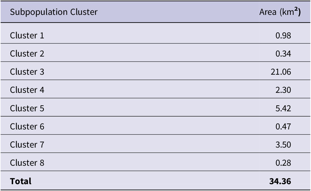
Distribution points were clustered into eight major subpopulations, with several outlying records scattered within the overall region (Figure 1). Due to the stochastic nature of the concaveman algorithm and R, metrics varied slightly among model runs but consistently found a total distribution area of c.34.36 km2 with the 100 m buffer applied. We dealt with some of this variability by using “set.seed(815)” to establish a repeatable pseudorandom instance for all metrics reported herein. Major subpopulations varied in size (as determined by the buffered concave polygons) with half of them < 1 km2 and the smallest cluster at 0.28 km2 (Table 1). The four largest subpopulations were 2.30 km2, 3.50 km2, 5.42 km2, and 21.06 km2, with the largest cluster overlapping broadly with the Amani Nature Forest Reserve (Figure 1). Approximately 61% of the species’ estimated distribution was accounted for by this single subpopulation cluster. Records were reported more consistently from these larger areas, with many smaller areas having few to no records in most years of the study (Figure 2; Table S1).
An elevational map (in metres) of the East Usambara Mountains and nearby ranges. Left: detections from Artisornis moreaui surveys overlaid, with darker areas denoting more overlapping detections. Right: with protected areas (outlined and grey-shaded polygons) and concave polygons of occurrence for Artisornis moreaui based on our study (white polygons) are shown. Note that protected areas and occurrence polygons are largely concordant, with protected areas covering much of this species range and areas of adjacent suitable habitat.
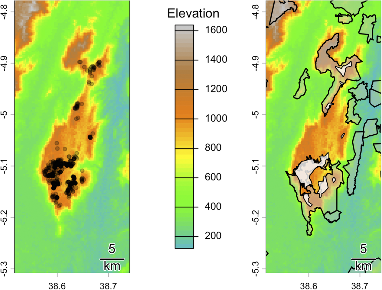
Figure 1. Long description
A two-panel topographical map set. Between the panels is a vertical elevation legend in metres, ranging from 200 (light blue) to 1600 (grey), with green representing 400 to 600 and orange representing 1000 to 1200. Both maps use a coordinate system with latitude on the Y-axis from -5.3 to -4.8 and longitude on the X-axis from 38.6 to 38.7.
* The left panel displays survey detections of Artisornis moreaui as black circular points. These points are heavily concentrated in the South-Central high-elevation orange zone, with a secondary, sparser cluster extending Northward along the mountain ridge.
* The right panel displays protected areas as grey-shaded polygons with black outlines and occurrence areas as white polygons. The largest protected area and occurrence polygon overlap significantly in the South-Central region. Smaller protected areas are scattered to the North and East.
* A 5 km scale bar is located in the bottom-right corner of both panels.
Area of each subpopulation cluster of Artisornis moreaui evaluated in this study
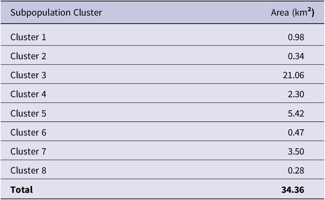
Table 1. Long description
The table consists of two columns: Subpopulation Cluster and Area in km 2.
* Cluster 1: 0.98
* Cluster 2: 0.34
* Cluster 3: 21.06
* Cluster 4: 2.30
* Cluster 5: 5.42
* Cluster 6: 0.47
* Cluster 7: 3.50
* Cluster 8: 0.28
* Total: 34.36
A plot of the number of observations of Artisornis moreaui per population cluster per year (left) and the spatial outlines of the clusters (right). Note that the two largest clusters—3 and 5—account for the majority of records, which is where surveys were repeated the most during the study period.
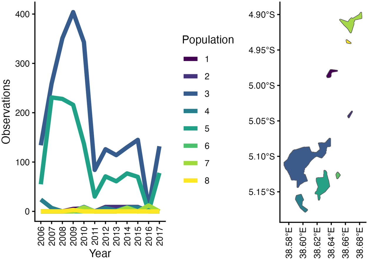
Figure 2. Long description
The graphic consists of two panels and a central legend.
Left Panel: A line graph titled Observations on the y-axis (0 to 400) and Year on the x-axis (2006 to 2017).
- Sub-population 3 (dark blue) shows a sharp increase from 150 in 2006 to a peak of 400 in 2009, followed by a steep decline to 100 in 2011, and fluctuating between 100 and 150 thereafter.
- Sub-population 5 (teal) starts at 60, peaks at 230 in 2007, maintains high levels until 2009, then drops sharply to 30 in 2011, with minor fluctuations below 100 until 2017.
- Sub-populations 1, 2, 4, 6, 7, and 8 remain consistently near the zero line throughout the study period.
Central Legend: A vertical list labeled Population with color-coded swatches numbered 1 through 8, ranging from dark purple to bright yellow.
Right Panel: A geographical map with Latitude on the y-axis (4.90 degrees South to 5.15 degrees South) and Longitude on the x-axis (38.58 degrees East to 38.68 degrees East).
- The largest cluster, Sub-population 3 (dark blue), is located in the Southwest quadrant.
- Sub-population 5 (teal) is located just East and South of Sub-population 3.
- Sub-population 7 (light green) and 8 (yellow) are small clusters in the Northeast.
- Sub-populations 1, 2, 4, and 6 appear as smaller, scattered polygons in the central and Eastern regions of the map.
Distribution models
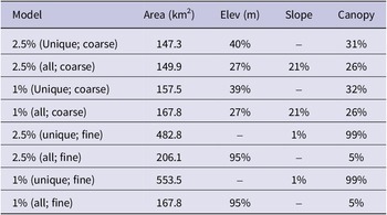
For all coarse-scale model scenarios, elevation was the most important predictor of species’ presence (with an average relative contribution of 39% in the 2.5% error coarse scale models with unique points), followed by canopy information (also with an average contribution of over 30% in some cases). Few other variables contributed more than 10% to model creation, namely the maximum potential evapotranspiration (third most important variable in unique locality models), slope (third most important variable for all observation models), and precipitation seasonality (bio15). Fine scale models—trained on only three variables—differed more strongly between the unique and all localities datasets, with the unique datasets being largely (c.99%) driven primarily by canopy data with some contribution of slope and all observation data being largely driven by elevation (c. 95%) and by canopy cover. In all models, 1% error models predicted a larger area than 2.5% error models. However, in coarse scale models, using unique localities only predicted a smaller distribution whereas in the fine scale models using all observations predicted smaller distributions (Table 2).
Select summary statistics for models used in these analyses. Model references error allowed (percent), points used (unique localities or all observations), and scale (coarse for large raster cell size, fine for small raster cell size). Elev = elevation
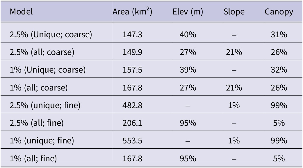
Table 2. Long description
The table consists of five columns: Model, Area in km 2, Elev in m, Slope, and Canopy.
* 2.5% (unique; coarse): area 147.3, elev 40%, slope -, canopy 31%.
* 2.5% (all; coarse): area 149.9, elev 27%, slope 21%, canopy 26%.
* 1% (unique; coarse): area 157.5, elev 39%, slope -, canopy 32%.
* 1% (all; coarse): area 167.8, elev 27%, slope 21%, canopy 26%.
* 2.5% (unique; fine): area 482.8, elev -, slope 1%, canopy 99%.
* 2.5% (all; fine): area 206.1, elev 95%, slope -, canopy 5%.
* 1% (unique; fine): area 553.5, elev -, slope 1%, canopy 99%.
* 1% (all; fine): area 167.8, elev 95%, slope -, canopy 5%.
Comparison of areas
We found that 77% of the distribution of A. moreaui, as determined via concave polygons, lies within protected areas. Despite the reported distribution of the species of 328 km2 in BirdLife (2025), the BirdLife distribution shapefile made available to us had an area of 179.7 km2 in the main part of the distributional polygon which encompassed 89% of the distribution of A. moreaui. Thus, there is an area of overprediction of 149.0 km2 within the BirdLife map. All our models likewise showed extensive overpredictions (Figure 3) but encompassed almost the entirety of the occupied distribution of the species. Interestingly, our coarse models omitted less of the species’ distribution (< 1%) than did our fine models (4%). Our 2.5% error map of unique localities at a coarse scale had an overprediction of 123.3 km2, while our fine scale maps had an overprediction of 191.8 km2 (Figure 3).
Species suitability in the East Usambara Mountains, as determined from our coarse scale 2.5% error unique locality model (left) and our fine scale 1% error all observations model (right); the models for each scale that predicted the smallest total area of distribution are presented. Each plot shows a dark black outline around the areas deemed “suitable” when we thresholded our binary models, and our concave distribution polygons are overlain in white with thin black outlines. Note how much more extensive the predicted area is for the fine scale model, and that the fine scale model lacks the connectivity shown in the coarse scale model.
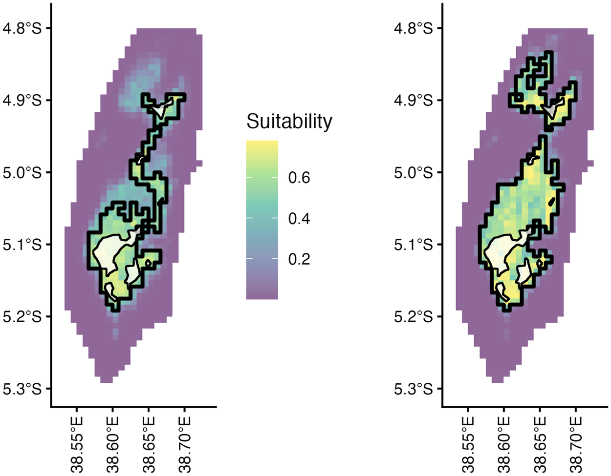
Figure 3. Long description
Two side-by-side geographical heat maps share a vertical Y-axis on the left and right edges ranging from 4.8 degrees South to 5.3 degrees South, and horizontal X-axes at the bottom ranging from 38.55 degrees East to 38.70 degrees East. A central legend titled Suitability uses a color gradient from purple (0.2) to yellow (0.6).
* Left Panel (Coarse Scale Model): Shows a continuous, elongated north-to-south distribution of suitability. The highest suitability (yellow) is concentrated in the Southwest. A thick black outline defines the suitable threshold, forming a single connected shape that narrows in the center. White concave polygons with thin black outlines are nested within the southern and northern sections.
* Right Panel (Fine Scale Model): Shows a more fragmented and extensive distribution. The thick black outline defines three distinct suitable areas: a small northern cluster, a tiny central point, and a large southern mass. The yellow high-suitability pixels are more widely dispersed throughout the southern mass compared to the left panel. The white concave polygons are in the same locations as the left panel but appear smaller relative to the expanded black-outlined suitable area.
Discussion
We found that the actual occupied area for A. moreaui is very small, at only c. 34 km2, a small fraction of BirdLife’s (2025) officially reported estimations, shapefiles, and areas that are predicted to be suitable for the species. Interestingly, we found that coarse scale models showed the smallest amount of overprediction; however, it is worth noting that these models used fewer variables than our fine scale models. While our models broadly encompass most or all the points and areas where this species is present, especially within protected areas, they substantially overestimate the distribution across the entirety of the East Usambaras. Our models also show the importance of elevation and canopy height for describing where this species occurs, well-defining all areas where this microendemic is present while simultaneously possessing overpredictions that suggest the influence of additional limiting factors not captured by the models.
Importance of modelling the distribution of Artisornis moreaui
Range and population size are strong predictors of extinction risk (Davies et al. Reference Davies, Margules and Lawrence2004; Gaston and Fuller Reference Gaston and Fuller2009; Purvis et al. Reference Purvis, Gittleman, Cowlishaw and Mace2000), and there is therefore strong international, regional, and local conservation and management interest for narrowly distributed and rare species such as A. moreaui (Davies et al. Reference Davies, Margules and Lawrence2004; IUCN 2024). Using our dataset of almost two decades of observations of this species, we present the most precise overview of this species’ distribution ever published. Furthermore, by incorporating ecological niche models, we provide a framework for identifying areas of priority for future conservation action to ensure the continued preservation of this taxon.
Importantly, all our models and precise distribution polygons suggest that published estimates of range size based on habitat and forest cover greatly overestimate the species’ distribution. More information, especially on historical records, would be needed to determine how accurately the niche models and published distributions truly capture the ecological niche of this warbler and the areas of possible occupancy when the forested areas were larger and continuous on the plateau. Interestingly, we found that the most important variables for describing this species were related to elevation and canopy height for all models. This concurs with our observations in the field, wherein A. moreaui prefers higher elevation forest, including modified habitats that abut the forest. However, only some models, namely those with all observations, highlighted the importance of slope for species presence, something we have noticed in the field as the species appears to avoid areas with rough, steep terrain.
Perhaps the most surprising finding in this analysis was the drastic difference between model performance in scenarios that included all observations versus only unique localities. While the difference was more minimal at coarser scales, it was much more pronounced at fine scales. This suggests that, as predictor variables occur at finer scales, the data that we use to train them should likewise increase. Such issues could be further mitigated by incorporating more landscape perspectives into these models, but the risks of overpredictions caused by preparing ‘classic’ niche models based on these fine-scale data are evident (Strimas-Mackey et al. Reference Strimas-Mackey, Hochachka, Ruiz-Gutierrez, Robinson, Miller and Auer2023).
The ecological niche and distribution of Artisornis moreaui
Only a few of these polygons defined as the distribution of the species show consistent occupancy. While the apparent over-dominance of two subpopulations is noteworthy (Figure 3), this pattern is largely an artefact of concentrated efforts of monitoring these locations. The reliability of relocating territories in the largest subpopulations (and the greater contiguous spatial extent of these subpopulations) indicates conservation attention should be focused on these core areas. Additionally, smaller subpopulations are largely within protected areas, including Nilo Nature Forest Reserve (Figs. 1), which we have repeatedly surveyed only three times, and yet despite limited surveys there still represents another stronghold for focused conservation efforts. Some of these smaller populations exist near the edges of these protected areas or in unprotected privately owned forest, areas subject to rapid degradation (Mtango and Kijazi Reference Mtango and Kijazi2014).
Overall, the predicted modelled distributions generally match ecological requirements reported for this species, as also confirmed by the actual distributions. The species is restricted primarily between 800–1100 m, with an upper limit of 1250 m at Nilo Nature Forest Reserve (Cordeiro Reference Cordeiro1998), inhabiting submontane forest on the plateau (Borghesio et al. Reference Borghesio, John, Mulungu, Mkongewa, Joho and Cordeiro2008; Cordeiro et al. Reference Cordeiro, Pohjonen and Mulungu2001). There, it inhabits areas with a high density of lianas, tangles, and vines, along the forest edge and large interior forest gaps (Cordeiro et al. Reference Cordeiro, Pohjonen and Mulungu2001; McEntee et al. Reference McEntee, Cordeiro, Joho and Moyer2005). It is possible that extensive forest fragmentation due to large-scale coffee and followed soon after by tea estates dating back to the pre-colonial times (Newmark Reference Newmark2002), explains much of the species distribution along the forest edge of the northern large fragment of Amani Nature Forest Reserve (i.e. subpopulation 3; Figure 1). This is difficult to discern without historical distribution data prior to fragmentation. Modified habitats, especially those fragmented or altered by local human populations, may influence the occupancy of the species, as indicated by the suitable environmental areas we highlight here that occur in deforested areas and lack any A. moreaui.
Habitat specialists are often negatively impacted by habitat degradation (Keinath et al. Reference Keinath, Doak, Hodges, Prugh, Fagan and Şekercioğlu2017; Morante-Filho et al. Reference Morante-Filho, Arroyo-Rodríguez and Faria2016), but some, like A. moreaui, can adapt to modified habitats such Lantana thickets at, or close to, the forest edge. These modified habitats are more subject to disturbance because they are often converted back to farmland after being abandoned for some time or, in this case, fast-growing Eucalypt plantations needed as firewood for the tea factories of the two tea estates in the area (John and Kabigumila Reference John and Kabigumila2007). This may explain why the predicted models indicate very low occupancy of a portion of non-forest habitat, which is primarily the satellite points above subpopulation 3 and near subpopulation 1 (Figures 1, 2). That this species occurs in Lantana thickets should be carefully considered as habitat it extends into from its primary niche and therefore considering it a “shrubland” species is inaccurate (BirdLife International 2018; Madge et al. 2020) and can impact how decision-makers develop conservation strategies for this species.
Conservation Implications
Our findings highlight how extensive, fine-scale assessments of globally threatened taxa are an effective approach for assessing their occupied range. Furthermore, our modelling pipelines illustrate ways in which different approaches may excessively inflate species distribution estimates. The extremely small observed distribution of this microendemic, along with the fragmentation of its primary habitat, qualifies this taxon as Endangered (BirdLife International 2018; Madge et al. 2020). Interestingly, while models of the distribution still indicate the taxon is extremely rare, we can therefore conclude that any management strategies to preserve the species in the future should prioritise a more focused approach on the eight core subpopulations we identified. However, managers should not ignore fringing subpopulations as these areas could be locations that displaced individuals from disturbed forest edges and secondary growth overspill into, at least on a more temporary basis until more prime territory is available. Furthermore, since its initial discovery in Nilo Nature Forest Reserve in 1994 (Cordeiro Reference Cordeiro1998), we began more expansive population surveys and monitoring in this region beginning in 2010. Though sampled infrequently due to funding limitations (see Atkinson et al. Reference Atkinson, Diop, Robinson, Altwegg, Amar and Barber2026), our coverage expanded our knowledge of its distribution there, primarily from the middle to the south of Nilo Nature Forest Reserve. This also directed the team to survey the Derema corridor, where subpopulation 2 was found. Based on the predicted model (Figure 2), we would advocate for more intensive surveys of parts of the Derema corridor and Nilo Nature Forest Reserve. While more records from these locations are likely to raise the population beyond 200-400 individuals estimated to exist (BirdLife International 2025), the extremely narrow distribution and fragmented populations would not change the threat status of this species. A review of eight biodiversity hotspots in the tropics, which included the East Usambara Mountains as part of the Eastern Afromontane hotspot, found that protected areas have a measurable conservation impact on forest-dependent, endemic, and globally threatened and Near Threatened birds (Cazalis et al. Reference Cazalis, Princé, Mihoub, Kelly, Butchart and Rodrigues2020). It is therefore promising that the bulk of the population of this habitat specialist survives in two nature reserves, which have the highest protection in the region (Cazalis et al. Reference Cazalis, Princé, Mihoub, Kelly, Butchart and Rodrigues2020). If corridors are added to connect some of the submontane fragments, as proposed by Newmark et al. (Reference Newmark, Jenkins, Pimm, McNeally and Halley2017), particularly the area we highlighted between Nilo and Amani Nature Forest Reserves, then maintenance of these fragmented subpopulations could be enhanced (Newmark et al. Reference Newmark, Jenkins, Pimm, McNeally and Halley2017). Furthermore, these results update the species’ factsheets on the IUCN Red List and BirdLife International platforms (https://www.iucnredlist.org/) which could help raise more acute conservation awareness of this species’ threats. Lastly, if funding is secured through more innovative approaches in the region (see Atkinson et al. Reference Atkinson, Diop, Robinson, Altwegg, Amar and Barber2026), we recommend that continued long-term monitoring of A. moreaui, as well as other globally threatened species, be maintained on the already established fixed-point transects.
Supplementary material
The supplementary material for this article can be found at http://doi.org/10.1017/S0959270926100574.
Acknowledgements
Conservation research and work on this species was supported by the RSPB from 2005 to 2017 through multiple small grant initiatives, including at least two BirdFair awards. BirdLife shapefiles were made available by Mark Balman on behalf of BirdLife International. The team wishes to express sincere gratitude to Julius Arinaitwe from BirdLife International’s Africa office and Alice Ward-Francis (RSPB), for their extensive logistic support. Luca Borghesio is greatly credited for developing the fixed point transects and training of the field team. Luis Carlos Beltrán provided extensive assistance with data organisation and quality checking. Others for which we are grateful for logistical and field assistance include Pius Exper, Lota Melamari, Elia Mulungu, Stiga Munisi, Mercy Nambu, Fadhili Njilima, Kyonjola Nsajigwa, and Festo Semanini. Jacob C. Cooper was funded in part by the Institutional Research and Academic Career Development Award (IRACDA; NIH 2K12GM063651) to the University of Kansas. The Wildlife Conservation Society of Tanzania spearheaded the setup of the initial field surveys and BirdLife Tanzania oversaw the last few years up to 2017 when funding ended. Permission to conduct this research and conservation work was granted by the Tanzania Wildlife Research Institute (TAWIRI), Tanzania Commission for Science and Technology and Amani and Nilo Nature Forest Reserves. This manuscript was reviewed by TAWIRI prior to submission.




 Open access

