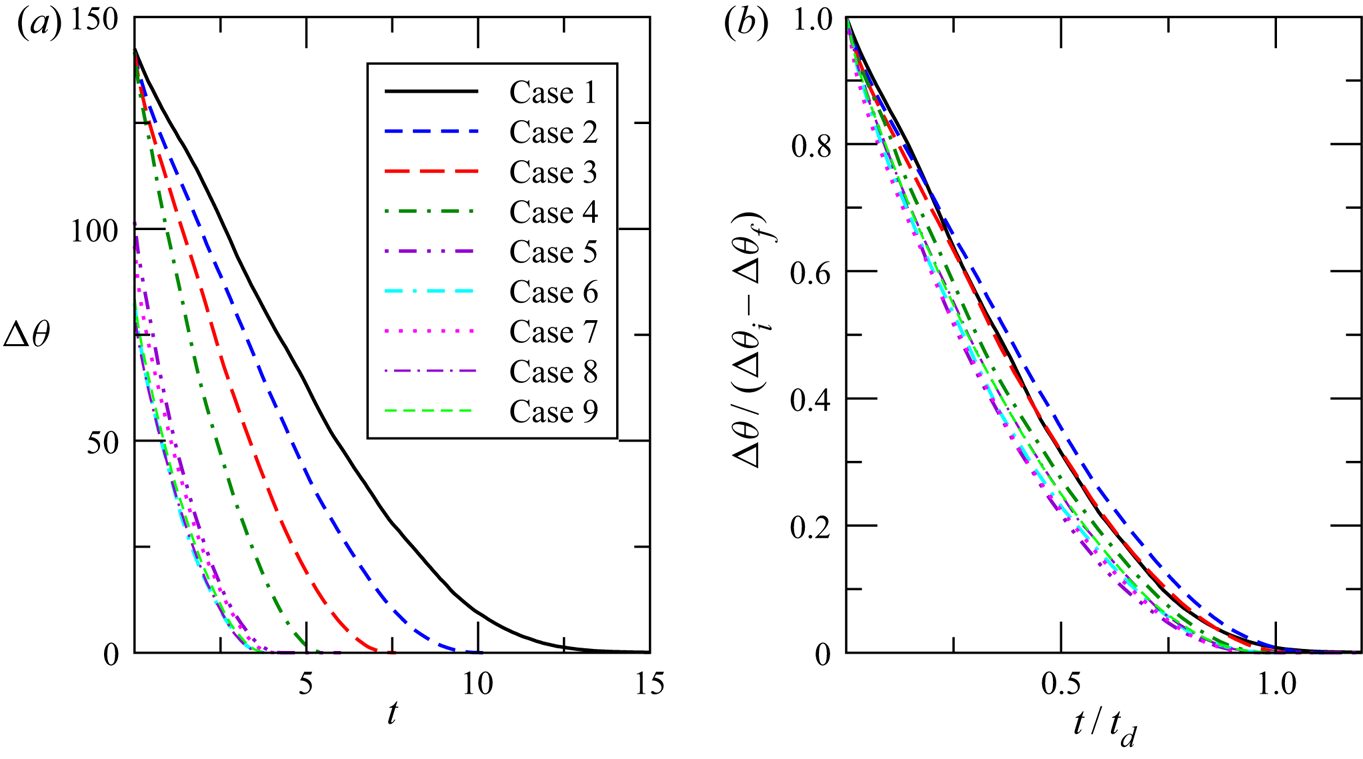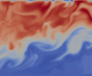


1. Introduction
In this study we investigate the time evolution of thermally stratified open-channel flow in response to the imposition of a cooling flux at the upper free surface. The initial stratification is gradually broken down by a combination of shear-driven turbulence from the bottom of the channel and turbulence generated by natural convection from the top. As such, the flow evolves from an initial stably stratified state, in which turbulent mixing is strongly damped, to an unstably stratified flow, in which convective turbulence generated at the top of the channel interacts with shear-generated turbulence from the channel bottom, leading to energetic mixing.
A particular motivation of the current study is a need to address ecosystem issues that result from the occurrence of thermal stratification in turbid, low-land rivers such as the Murray and Murrumbidgee Rivers of south-eastern Australia. Here, a combination of high solar radiation and turbidity and low flow rates often lead to persistent stable stratification (Bormans et al. Reference Bormans, Maier, Burch and Baker1997; Bormans & Webster Reference Bormans and Webster1997). Persistence of strong stable stratification for more than a few days has been identified as a key risk factor for algal blooms (Sherman et al. Reference Sherman, Webster, Jones and Oliver1998; Webster et al. Reference Webster, Sherman, Bormans and Jones2000). On the other hand, the sudden breakdown of strong persistent stable stratification was found to be the main cause of two recent mass fish kill events in the Darling River system in south-eastern Australia (Moritz et al. Reference Moritz, Blackall, Davis, Flannery, Godden, Head, Jackson, Kingsford, Wheeler and Williams2019).
Thermally stratified open-channel flow is an appropriate model for these rivers, which have a moderate to high width to depth ratio (typically between 8:1 and 20:1) with a relatively flat bed (see Schumm Reference Schumm1968; Bormans et al. Reference Bormans, Maier, Burch and Baker1997). Flow velocities during periods of strong stratification are low ( $2\text {--}6\ \textrm {cm}\ \textrm {s}^{-1}$) while the channel depth is typically
 $3\text {--}10$ m (Bormans et al. Reference Bormans, Maier, Burch and Baker1997; Sherman et al. Reference Sherman, Webster, Jones and Oliver1998), implying a Froude number less than unity and subcritical flow. Typical water temperature is in the range
 $20\text {--}30\,^{\circ }\textrm {C}$, well above the temperature of maximum density, so an increase in temperature will always correspond to a decrease in density.
Williamson et al. (Reference Williamson, Armfield, Kirkpatrick and Norris2015) present a direct numerical simulation model for the statistically steady equilibrium state approached by a river or channel under the influence of day-time solar heating. Thermal stratification due to progressive absorption of solar radiation is represented by an internal heat source that decays exponentially with depth following the Beer–Lambert law, with the attenuation coefficient relative to channel depth set high enough to ensure that radiation reaching the channel bottom is negligible. This is typical of the situation occurring in the target rivers where the attenuation coefficient is usually between 1.5 and 2.5 m $^{-1}$ (Bormans & Webster Reference Bormans and Webster1998).
In a previous study, (Kirkpatrick et al. Reference Kirkpatrick, Williamson, Armfield and Zecevic2019, henceforth KWAZ) we investigated the transient evolution of this flow when the solar heat source is removed and the flow allowed to evolve in time with no heat flux through the upper or lower boundaries. This model represents the situation in which solar forcing stops, due for example to an increase in cloud cover, while atmospheric conditions are such that surface heat fluxes are small. We found that turbulence generated by shear due to friction at the channel bottom breaks down the stratification and the flow evolves gradually toward an isothermal turbulent open-channel flow state. The rate at which this destratification proceeds was found to scale with a friction Richardson number  $Ri_{\tau }$ in which the velocity scale is the friction velocity
 $u_{\tau }$ at the channel bottom.
In the current study we use a similar approach, but add a surface cooling flux at the same time as the internal heat source is removed. As such, this study is pertinent to the situation in which internal solar heating of a thermally stratified river is replaced by a surface cooling forcing due to sensible, evaporative and long-wave radiative emission, as typically occurs at night (Bormans et al. Reference Bormans, Maier, Burch and Baker1997) or as the result of the passage of a cold front (Reinfelds & Williams Reference Reinfelds and Williams2012). Net surface heat fluxes depend on weather conditions, but summer-time measurements in the target rivers show that they are typically between 200 and  $600\ \textrm {W}\;\textrm {m}^{-2}$ and hence comparable to the day-time clear sky solar heating flux averaged over daylight hours of
 ${\approx}400 \ \textrm {W}\ \textrm {m}^{-2}$ (Bormans et al. Reference Bormans, Maier, Burch and Baker1997; Bormans & Webster Reference Bormans and Webster1998). Those authors also show that wind forcing can play a significant role in mixing in thermally stratified rivers. The effects of wind forcing are left to a future study.
We anticipate that the findings presented here may also be of relevance in a number of other environmental and geophysical contexts. In KWAZ we demonstrated close similarities between the stratified turbulence in the central region of our channel flow with sheared stratified turbulence observed in large scale geophysical and environmental flows. In particular, our simulations demonstrated excellent agreement with various parameterisations for oceanic diapycnal mixing (Osborn & Cox Reference Osborn and Cox1972; Osborn Reference Osborn1980; Ivey, Bluteau & Jones Reference Ivey, Bluteau and Jones2018), a number of scalings based on Monin–Obukhov theory (Chung& Matheou Reference Chung and Matheou2012; Scotti & White Reference Scotti and White2016; Zhou, Taylor & Caulfield Reference Zhou, Taylor and Caulfield2017) and the classic Monin–Obukhov stability functions determined by Dyer (Reference Dyer1974) from atmospheric field data.
Within these contexts there are a number of situations that are similar to the flow considered here. In the ocean, tidally forced continental shelf seas are subject to bed shear from below and radiative heating from above (Simpson & Hunter Reference Simpson and Hunter1974) and may also be subject to strong surface cooling as the result of the passage of cold fronts (Zikanov, Slinn & Dhanak Reference Zikanov, Slinn and Dhanak2002). In the atmospheric context, boundary layer stratus clouds such as stratocumulus typically sit partially within a stable temperature inversion and are subject to evaporative and long-wave radiative cooling at the cloud top (see Mellado et al. Reference Mellado, Stevens, Schmidt and Peters2009; Wood Reference Wood2012; Mellado Reference Mellado2017, for example). In the case of marine cumulus clouds, in addition to the capping inversion, the boundary layer itself is often stably stratified (Paluch & Lenschow Reference Paluch and Lenschow1991). Mixing in water clouds is complicated by thermodynamic heat exchanges due to evaporation and condensation of water droplets. These phase change effects are absent in smoke clouds, however (see Bretherton et al. Reference Bretherton, Macvean, Bechtold, Chlond, Cotton, Cuxart, Cuijpers, Mhairoutdinov, Kosovic and Lewellen1999; de Lozar & Mellado Reference de Lozar and Mellado2013, for example) which have been shown to have significant impacts on climate (Koren et al. Reference Koren, Kaufman, Remer and Martins2004).
With regard to previous work, we are not aware of any previous studies of the transient evolution of thermally stratified open-channel flow in response to surface cooling. Most closely related are studies of surface-driven free convection penetrating into a stationary fluid layer with stable background stratification, including experimental (Deardorff et al. Reference Deardorff, Willis and Stockton1980; Fernando & Little Reference Fernando and Little1990), numerical (Zikanov, Slinn & Dhanak Reference Zikanov, Slinn and Dhanak2002; Fedorovich, Conzemius & Mironov Reference Fedorovich, Conzemius and Mironov2004) and field studies (Bouffard et al. Reference Bouffard, Zdorovennova, Bogdanov, Efremova, Lavanchy, Palshin, Terzhevik, Vinnå, Volkov and Wüest2019). Also related is an experimental investigation of surface cooling by Sayler & Breidenthal (Reference Sayler and Breidenthal1998) aimed at simulating entrainment due to cloud-top cooling in stratiform clouds. These studies have found that turbulence statistics and bulk quantities such as entrainment rate scale in terms of a convection velocity  $ {w}_*$ (Deardorff Reference Deardorff1970) that is a function of the surface buoyancy flux and mixed layer height. Deardorff et al. (Reference Deardorff, Willis and Stockton1980) found that the entrainment rate
 $E$ scales with a convection Richardson number
 $Ri_*$ according to a simple power law relationship,
 \begin{equation} \frac{E}{{w}_* } = C Ri_{*}^{-1}. \end{equation}
This and similar scaling relationships based on  $ {w}_*$ have been used extensively to parameterise thermal convection processes that occur in the atmospheric boundary layer, as well as in large water bodies such as oceans and lakes (see Marshall & Schott Reference Marshall and Schott1999; Fedorovich et al. Reference Fedorovich, Conzemius and Mironov2004; Ihle & Niño Reference Ihle and Niño2012; Bouffard & Wüest Reference Bouffard and Wüest2019, for reviews).
The remainder of this paper is structured as follows. Section 2 describes the mathematical formulation of the problem including the governing equations and non-dimensionalisations used. The direct numerical simulation (DNS) code and details of the numerical simulations including the parameter ranges considered and statistical methods used are given in § 3. In § 4 we present flow visualisations and vertical profiles of a selection of turbulence statistics and use this to describe the time evolution of the flow from its initial stably stratified equilibrium state to a destratified state in response to surface cooling. Based on these observations, in § 5 we use scaling analysis to determine a relationship for the destratification rate in terms of friction and convection Richardson numbers,  $Ri_{\tau }$ and
 $Ri_*$. We then show that this relationship can be integrated to give a formula for the time taken for destratification as a function of the dominant velocity scales and initial stratification and discuss possible application of these findings for predicting destratification rates in thermally stratified riverine flows. Section 6 summarises the major findings of the paper.
2. Problem formulation
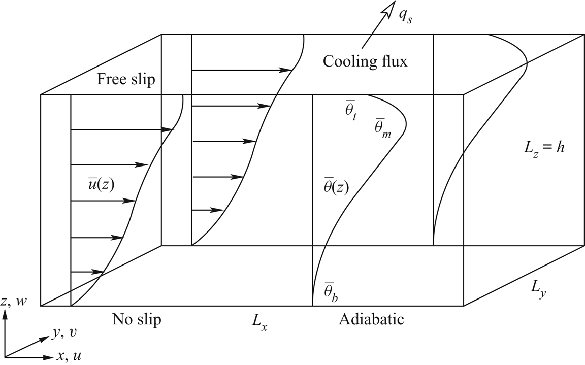
The initial state for the time-evolving flow is the statistically steady heated equilibrium state described by Williamson et al. (Reference Williamson, Armfield, Kirkpatrick and Norris2015). As shown in figure 1, the flow is an open-channel flow with a free-slip impermeable boundary at the upper surface, an adiabatic, no-slip wall at the lower surface and periodic boundaries in the streamwise and spanwise directions. The flow is driven by a constant pressure gradient in the streamwise direction.
Schematic of the flow with surface cooling.

In the heated equilibrium flow the upper boundary is adiabatic and a depth-dependent volumetric heat source  $\tilde {q}_r(\tilde {z})$ following the Beer–Lambert law is used to represent radiative heating:
 \begin{equation} \tilde{q}_r(\tilde{z}) = \tilde{I}_s \tilde{\alpha}\,\textrm{e}^{(\tilde{z} - \tilde{h})\tilde{\alpha}}. \end{equation}
Here,  $\tilde {I}_s$ is the radiative heat flux through the upper boundary,
 $\tilde {h}$ the channel height and
 $\tilde {\alpha }$ an attenuation coefficient.
Throughout this paper a tilde  $\tilde {\cdot }$ over a variable indicates a dimensional quantity, whereas a variable with no tilde is non-dimensional. For clarity, variables in figure 1 are shown in their non-dimensional form.
The time-evolving destratifying flow uses the same domain and boundary conditions, except that the volumetric radiative heat source  $\tilde {q}_r$ is removed and a constant cooling flux
 $\tilde {q}_s$ is applied at the top boundary, defined as positive for heat flux out of the domain.
The temperature field  $\tilde {\Theta }(\tilde {\boldsymbol {x}},\tilde {t})$ can be decomposed into a time varying domain-averaged component
 $\tilde {\Theta }_v(\tilde {t})$ and a fluctuating component
 $\tilde {\theta }(\tilde {\boldsymbol {x}},\tilde {t})$:
 \begin{equation} \tilde{\Theta}(\tilde{\boldsymbol{x}},\tilde{t}) = \tilde{\Theta}_v(\tilde{t}) + \tilde{\theta}(\tilde{\boldsymbol{x}},\tilde{t}). \end{equation}
For the heated equilibrium state flow the domain-averaged temperature increases with time according to
 \begin{equation} \frac{\textrm{d}\tilde{\Theta}_v}{\textrm{d}\tilde{t}} = \frac{\tilde{Q}_r}{\tilde{\rho}_b \tilde{c}_p}, \end{equation}
where  $\tilde {\rho }_b$ and
 $\tilde {c}_p$ are a reference density and the specific heat of the fluid, and
 $\tilde {Q}_r$ the domain-averaged radiative heat source,
 \begin{equation} \tilde{Q}_r = \frac{1}{\tilde{h}}\int_0^{\tilde{h}}\tilde{q}_r(\tilde{z})\,\textrm{d}\tilde{z}. \end{equation}
For the destratifying flow,  $\tilde {\Theta }_v(\tilde {t})$ decreases with time due to the boundary cooling flux according to
 \begin{equation} \frac{\textrm{d}\tilde{\Theta}_v}{\textrm{d}\tilde{t}} = -\frac{\tilde{q}_s}{\tilde{\rho}_b \tilde{c}_p \tilde{h}}. \end{equation}
Williamson et al. (Reference Williamson, Armfield, Kirkpatrick and Norris2015) show that the statistically steady heated equilibrium state can be defined in terms of a friction Reynolds number  ${\textit {Re}}_{\tau ,0}$, Prandtl number
 $Pr$, a stability parameter
 $\lambda$ and a dimensionless attenuation coefficient
 $\alpha$, defined as
 \begin{equation} {\textit{Re}}_{\tau,0} = \frac{\tilde{u}_{\tau,0} \tilde{h}}{\tilde{\nu}}, \quad Pr = \frac{\tilde{\nu}}{\tilde{\kappa}}, \quad \lambda = \frac{\tilde{\beta} \tilde{g} \tilde{\Theta}_{N}\tilde{h}}{\tilde{u}_{\tau,0}^2}, \quad \alpha = \tilde{\alpha} \tilde{h}. \end{equation}
Here,  $\tilde {u}_{\tau ,0}$ is the friction velocity at the channel bottom,
 $\tilde {\nu }$ the kinematic viscosity,
 $\tilde {\kappa }$ the thermal diffusivity,
 $\tilde {\beta }$ the coefficient of thermal expansion,
 $\tilde {g}$ gravitational acceleration and
 $\tilde {\Theta }_{N}$ a characteristic temperature scale defined as
 \begin{equation} \tilde{\Theta}_{N} = \frac{\tilde{Q}_{N} \tilde{h}}{\tilde{\rho}_b \tilde{c}_p \tilde{u}_{\tau,0}} , \end{equation}
where
 \begin{equation} \tilde{Q}_{N} = \frac{1}{\tilde{h}^2}\int_0^{\tilde{h}}(\tilde{Q}_r-\tilde{q}_r(\tilde{z}))(\tilde{h} - \tilde{z})\,\textrm{d}\tilde{z} \end{equation}
is a characteristic volumetric heat source associated with the radiative forcing.
A subscript 0 is used here for  ${\textit {Re}}_{\tau ,0}$ and
 $\tilde {u}_{\tau ,0}$ to indicate that these are associated with the initial equilibrium state. This distinction is necessary because
 $\tilde {u}_{\tau }$ and hence
 ${\textit {Re}}_{\tau }$ change due to changes in the turbulence structure of the flow as it destratifies. In the initial state, the friction coefficient
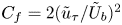 $C_f = 2( \tilde {u}_{\tau }/\tilde {U}_b )^2$ (where
 $\tilde {U}_b$ is the bulk velocity) is reduced relative to the neutral or unstably stratified flow at the same
 ${\textit {Re}}_{\tau }$. With our model, in which the flow is driven by a constant pressure gradient,
 $\tilde {u}_{\tau }$ increases initially in response to destratification, before decreasing again in later stages of the flow evolution as the flow decelerates until
 $\tilde {u}_{\tau }$ is again in balance with the applied pressure gradient. The increase in
 $\tilde {u}_{\tau }$ in the simulations presented here is in the range 20 %–30 %. The effect of stratification on
 $C_f$ in wall bounded flows has been noted by numerous authors (for example, Arya Reference Arya1975; Armenio & Sarkar Reference Armenio and Sarkar2002; Taylor, Sarkar & Armenio Reference Taylor, Sarkar and Armenio2005).
In KWAZ we found the dominant control parameters determining the behaviour and turbulence properties of the time-evolving flow with no surface cooling to be  ${\textit {Re}}_{\tau }$,
 $Pr$ and a friction Richardson number defined as
 \begin{equation} Ri_{\tau} = \frac{\tilde{\beta} \tilde{g} \Delta \tilde{\theta} \tilde{h}}{\tilde{u}_{\tau}^2}. \end{equation}
Here, 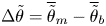 $\Delta \tilde {\theta } = \overline {\tilde {\theta }}_{m} - \overline {\tilde {\theta }}_{b}$, where
 $\overline {\tilde {\theta }}_{m}$ is the maximum horizontally averaged temperature in the channel and
 $\overline {\tilde {\theta }}_{b}$ the horizontally averaged temperature at the channel bottom, as shown in figure 1. An overbar
 $\overline {\cdot }$ will be used throughout this paper to indicate a quantity in which the average is calculated over horizontal planes only. The temperature difference
 $\Delta \tilde {\theta }$ and consequently
 $Ri_{\tau }$ decrease progressively as the flow destratifies.
The parameters  ${\textit {Re}}_{\tau }$ and
 $Ri_{\tau }$ contain a single velocity scale,
 $\tilde {u}_{\tau }$. For the current flow, in which destratification is also driven by convection due to surface cooling, an additional non-dimensional parameter is required. The analogies between the penetrative convection component of our flow and the penetrative convection model investigated by Deardorff et al. (Reference Deardorff, Willis and Stockton1980) suggest that the convective component of our flow may also be expected to scale in terms of some form of convection velocity
 $\tilde {w}_*$ and Richardson number
 $Ri_*$. Following Deardorff et al. (Reference Deardorff, Willis and Stockton1980) we define a convection velocity scale,
 \begin{equation} \tilde{w}_* = \left(\frac{\tilde{\beta} \tilde{g} \tilde{q}_s \tilde{h}}{\tilde{\rho}_b \tilde{c}_p}\right)^{1/3}, \end{equation}
and convection Richardson number,
 \begin{equation} Ri_* = \frac{\tilde{\beta} \tilde{g} \Delta\tilde{\theta} \tilde{h}}{\tilde{w}_{*}^2}. \end{equation}
The channel height  $\tilde {h}$ is used as the length scale here in order to maintain consistency with the other non-dimensional parameters. This implies that the effect of convection is felt across the depth of the channel. The validity of this assumption will be discussed further in § 5.
The flow is governed by the Oberbeck–Boussinesq form of the equations for conservation of mass, momentum and energy for an incompressible fluid. These are written in non-dimensional Cartesian tensor form as
 \begin{gather} \frac{\partial u_j}{\partial x_j} = 0, \end{gather}
 \begin{gather}\frac{\partial u_i}{\partial t} + \frac{\partial u_i u_j}{\partial x_j} = -\frac{\partial p}{\partial x_i} + \nu\frac{\partial^2 u_i}{\partial x_j^2} + \delta_{i1} + \gamma \theta \delta_{i3}, \end{gather}
 \begin{gather}\frac{\partial \theta}{\partial t} + \frac{\partial \theta u_j}{\partial x_j} = \kappa\frac{\partial^2 \theta}{\partial x_j^2} + q_e. \end{gather}
Here,  $x_i$ are the Cartesian components of the position vector
 $\boldsymbol {x}$,
 $u_i$ are the components of the velocity vector
 $\boldsymbol {u}$,
 $t$ is the time,
 $p$ the pressure,
 $\nu$ dimensionless kinematic viscosity,
 $\kappa$ dimensionless thermal diffusivity and
 $\gamma$ a dimensionless buoyancy coefficient;
 $\delta _{ij}$ represents the Kronecker delta. Summation over repeated indices is assumed. The flow is driven by a constant uniform pressure gradient,
 $\delta _{i1}$, in the streamwise direction.
 $q_e$ is the internal volumetric heat source. The variables in the above equations are non-dimensionalised with respect to
 $\tilde {h}$,
 $\tilde {u}_{\tau ,0}$ and
 $\tilde {\Theta }_{N}$
 \begin{equation} \left.\begin{array}{c@{}} \displaystyle u=\dfrac{\tilde{u}}{\tilde{u}_{\tau,0}}, \quad \theta = \dfrac{\tilde{\theta}}{\tilde{\Theta}_{N}}, \quad p = \dfrac{\tilde{p}}{\tilde{\rho}_0 \tilde{u}_{\tau,0} ^2}, \quad x=\dfrac{\tilde{x}}{\tilde{h}}, \quad t = \dfrac{\tilde{u}_{\tau,0}}{\tilde{h}}\,\tilde{t},\\ \displaystyle \nu= \dfrac{1}{{\textit{Re}}_{\tau,0}}, \quad \kappa = \dfrac{1}{{\textit{Re}}_{\tau,0} Pr}, \quad \gamma = \dfrac{\tilde{\beta}\tilde{g}\tilde{\Theta}_{N}\tilde{h}}{\tilde{u}_{\tau,0} ^2}. \end{array}\right\} \end{equation}
The internal volumetric heat source for both cases is set such that the net heat gain of the system is zero:
 \begin{equation} \left.\begin{array}{cc@{}} \displaystyle q_e({z}) = \dfrac{\tilde{q}_r(\tilde{z}) - \tilde{Q}_r}{\tilde{Q}_{N}} & \mbox{equilibrium flow},\\ \displaystyle q_e = \dfrac{\tilde{q}_s/\tilde{h}}{\tilde{Q}_{N} } & \mbox{destratifying flow}. \end{array}\right\} \end{equation}
This ensures that the domain-averaged temperature,  $\Theta _v$, of the computed solutions remains constant. Boundary conditions for the bottom (
 $z=0$) and top (
 $z=1$) boundaries are
 \begin{equation} \left. \begin{array}{lll} \displaystyle z = 0: & \displaystyle u = v = w = 0, & \displaystyle \dfrac{\partial \theta}{\partial z} = 0, \\ \displaystyle z = 1: & \displaystyle \dfrac{\partial u}{\partial z} = \dfrac{\partial v}{\partial z} = 0, \ w = 0, & \displaystyle \dfrac{\partial \theta}{\partial z} = -q_s/\kappa, \end{array}\right\} \end{equation}
where
 \begin{equation} q_s = \frac{\tilde{q}_s}{\tilde{Q}_{N} \tilde{h}}. \end{equation}
The variables and parameters defining the flow written in terms of the non-dimensionalisation scheme above are summarised below
 \begin{equation} \left. \begin{array}{c@{}} \displaystyle {\textit{Re}}_{\tau} = \dfrac{{u}_{\tau} h}{\nu}, \quad Ri_{\tau} = \dfrac{\gamma \Delta{\theta} h}{{u}_{\tau}^2}, \quad Ri_* = \dfrac{\gamma \Delta{\theta} h}{{w}_*^2}, \quad Pr = \dfrac{\nu}{\kappa}, \\ \displaystyle {u}_{\tau}({t}) =\dfrac{\tilde{u}_{\tau}(\tilde{t})}{\tilde{u}_{\tau,0}}, \quad h=\dfrac{\tilde{h}}{\tilde{h}}=1, \quad {w}_* = \dfrac{\tilde{w}_*}{\tilde{u}_{\tau,0}} = \left(\gamma q_s {h}\right)^{1/3}, \quad \Delta{\theta} = \overline{{\theta}}_{m} - \overline{{\theta}}_{b}. \end{array}\right\} \end{equation}
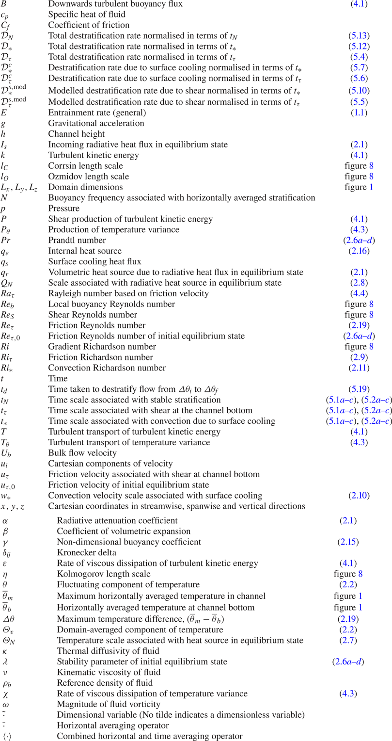
For reference, a table of symbols is given in table 3.
Table of symbols.

3. Method
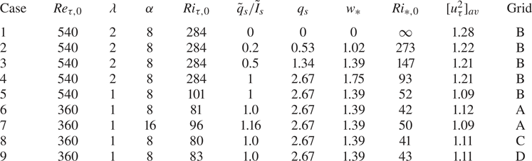
The flow cases analysed in this paper are shown in table 1. Initial conditions are the heated equilibrium states, generated in the same manner as in KWAZ. Simulations were performed using the PUFFIN code (Kirkpatrick Reference Kirkpatrick2002). The equations are discretised in space using a finite volume formulation on a non-uniform, staggered, Cartesian grid. The spatial discretisation uses fourth-order central differences for the advection terms in the momentum and energy equations. All other terms are discretised using second-order central differences. The equations are integrated in time using a second-order accurate fractional step method with mass conservation enforced using a pressure-correction method. The time step  $\Delta t$ was adjusted automatically to ensure that the maximum Courant number
 $({\Delta t u_i}/{\Delta x_i})$ in the domain remained in the range 0.18–0.2. Here,
 $\Delta x_i$ is the cell width in the direction of the velocity component
 $u_i$. This limit was determined from temporal convergence tests. We refer the reader to KWAZ for full details of the numerical methods used.
Simulation parameters defined in terms of initial heated equilibrium state and surface cooling. Note that  $\lambda \equiv \gamma$. Subscript
 $0$ indicates the average values of parameters for the equilibrium state. Here,
 $[ {u}_{\tau }^2]_{av}$ is the average value of
 $u_{\tau }^2$ measured in the simulations during the destratification process.

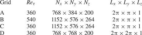
The domain and grid dimensions used are shown in table 2. A domain with dimensions  $2\pi \times \pi \times 1$ in the
 $x$,
 $y$ and
 $z$ directions, respectively, was used for all except one simulation which used a wider domain with dimensions
 $2\pi \times 2\pi \times 1$. The grid is uniform in the
 $x$ and
 $y$ directions. Here, the grid cell sizes in viscous wall units are
 $\Delta x^+_0 = \Delta y^+_0 = 2.95$. In the
 $z$ direction the grid is stretched from
 $\Delta z^+_0 = 0.36$ at the bottom boundary, to
 $\Delta z^+_0 = 2.2$ for
 $0.4 \le z \le 0.8$, and then down to
 $\Delta z^+_0 = 0.9$ at the upper boundary. These values are based on the initial Reynolds number of the simulation and hence increase during the simulation proportional to changes in friction velocity. The maximum increase in
 $ {u}_{\tau }$ is approximately 20 % for the
 $\lambda = 1$ cases and 30 % for the
 $\lambda = 2$ cases.
Grids and domain sizes used for each Reynolds number.

Resolution relative to the Kolmogorov scale  $\eta$ can be estimated from the plot of Kolmogorov scale given in figure 8 for Case 5. For this case the grid size in the
 $x$ and
 $y$ directions is
 $\Delta x = \Delta y = 5.5 \times 10^{-3}$ while in the
 $z$ direction the grid varies from
 $\Delta z = 7\times 10^{-4}$ at the bottom boundary, to
 $\Delta z = 4 \times 10^{-3}$ for
 $0.4 \le z \le 0.8$, and then to
 $\Delta z = 1.7\times 10^{-3}$ at the upper boundary. Vertical profiles of the Kolmogorov scale (figure 8) show that the minimum values of
 $\eta$ range from
 $\eta \approx 2.2 \times 10^{-3}$ close to the bottom boundary to
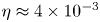 $\eta \approx 4 \times 10^{-3}$ in the central region of the channel and
 $\eta \approx 5.5 \times 10^{-3}$ close to the top surface. This is very similar to the values for the flow without surface cooling presented in KWAZ. The main difference is the region close to the top surface where the Kolmogorov scale is approximately 30 % smaller due to the increased intensity of the turbulence in this region resulting from the enhancement of turbulence production by descending plumes.
Thus the grid cell size in the horizontal directions relative to the Kolmogorov scale ranges from approximately  $\Delta x / \eta = \Delta y / \eta \approx 2$ close to the bottom boundary, to
 $\Delta x / \eta = \Delta y / \eta \approx 1.5$ in the central region and then
 $\Delta x / \eta = \Delta y / \eta \approx 1$ close to the upper surface. In the vertical direction,
 $\Delta z / \eta \approx 0.3$ close to the bottom boundary,
 $\Delta z / \eta \approx 1$ in the central region and
 $\Delta z / \eta \approx 0.3$ close to the upper surface. Similar ratios apply to the other cases. With our fourth-order spatial discretisation scheme and this degree of resolution the simulations are expected to resolve scales of motion of the order of the Kolmogorov scale for the Prandtl number tested.
Cases 1–6 represent the basic test cases that give a sweep of different parameters in order to test the scalings developed in § 5. The scaling analysis focuses on the effects of  $Ri_{\tau }$ and
 $Ri_*$. Both of these parameters sweep from the initial values given in table 1 to zero when
 $\Delta {\theta } = 0$ and the flow is fully destratified. Thus the simulations give a significant variation in
 $Ri_{\tau }$ and
 $Ri_*$ allowing us to accurately test the scalings developed in terms of these parameters.
The range of  ${\textit {Re}}_{\tau }$ is much smaller than the ranges of
 $Ri_{\tau }$ and
 $Ri_*$ and is included here in order to check for any substantial Reynolds number effects on the scaling relations. In KWAZ we also included a range of Prandtl numbers (
 $Pr = 0.5\text {--}1$) and found the destratification rate for the flow without surface cooling to be a function of
 $Pr$. The small
 $Pr$ range investigated was, however, insufficient to determine a quantitative scaling relationship with respect to this parameter. In the current study we acknowledge a probable
 $Pr$-dependence for the cases with surface cooling but, to ensure that our mesh resolution is sufficient, we restrict our investigation to
 $Pr = 0.71$. This is a typical value for air and was chosen so that our results might be directly applicable in relation to low
 ${\textit {Re}}_{\tau }$ and
 $Pr$ industrial flows or laboratory experiments in which air is the fluid.
The issue of matching Reynolds and Prandtl numbers of numerical or experimental investigations with those in intended large scale flow applications has been discussed at length in the literature with respect to both stably stratified shear flows (see Fernando Reference Fernando1991; Strang & Fernando Reference Strang and Fernando2001; Williamson, Kirkpatrick & Armfield Reference Williamson, Kirkpatrick and Armfield2018, for example) and penetrative convection (see for example, Fernando & Little Reference Fernando and Little1990; Sayler & Breidenthal Reference Sayler and Breidenthal1998; Bretherton et al. Reference Bretherton, Macvean, Bechtold, Chlond, Cotton, Cuxart, Cuijpers, Mhairoutdinov, Kosovic and Lewellen1999; Jonker & Jiménez Reference Jonker and Jiménez2014). Due to the convenience of using water for experiments, many laboratory investigations take an approach opposite to that often taken in numerical simulations, using moderate to high Prandtl (or Schmidt) number water-based experiments to model low Prandtl number gaseous flows such as the atmospheric boundary layer. The experiment used by Deardorff et al. (Reference Deardorff, Willis and Stockton1980) to determine the entrainment relation (1.1), for example, was done using thermally stratified water ( $Pr \approx 6$), while its intended application was the atmospheric boundary layer, where it has been used extensively to model entrainment (see for example, Betts & Ball Reference Betts and Ball1994; Angevine et al. Reference Angevine, Grimsdell, Hartten and Delany1998; Hägeli, Steyn & Strawbridge Reference Hägeli, Steyn and Strawbridge2000; Fedorovich, Conzemius & Mironov Reference Fedorovich, Conzemius and Mironov2004). Jonker & Jiménez (Reference Jonker and Jiménez2014) present a recent study of the dependence of this scaling on
 $Pr$. They found that the basic form of the scaling relation,
 $E=C Ri_*^{-1}$, provides a good match with measurements in experiments performed over a wide range of Prandtl and Schmidt numbers, but that the coefficient
 $C$ varies considerably. It is also worth noting here that there is a difference in the dynamics of scalar transport at small scales when
 $Pr < 1$ and
 $Pr > 1$. For
 $Pr < 1$ scalar variance is transferred to the Obukhov–Corrsin scale by inertial subrange motions, whereas, for
 $Pr > 1$, scalar variance is transferred from the Kolmogorov scale to the Batchelor scale by straining (Batchelor Reference Batchelor1959).
In § 5 we develop scaling relations with a similar form to (1.1) for the rate of destratification of thermally stratified channel flow as a function of  $Ri_{\tau }$ and
 $Ri_*$ and show that gives a good prediction of our low
 $Pr$ simulation results. Given that this relation is developed based on physical arguments related to ratios of time scales, the hope here is that any dependence of this relation on
 $Pr$ may also be restricted to the magnitude of the coefficients.
In KWAZ we found the effects of initial conditions on the flow with no surface cooling to be confined to an initial period in which the flow ‘relaxes’ from the heated equilibrium state in which buoyancy fluxes are balanced by the internal potential energy sink associated with the radiative heating, to the new time-evolving state in which a large portion of the channel is in local energetic equilibrium. Case 7, which has twice the attenuation coefficient  $\alpha$ of the other cases is included in the current study to check for any substantial effect of initial conditions on the flow with surface cooling. As discussed in KWAZ, higher
 $\alpha$ results in greater absorption of radiation which leads to a higher temperature gradient and increased stability close to the surface. Dimensionless attenuation coefficients in the range 4–20 are typical of the thermally stratified rivers of interest here, so the range
 $\alpha = 8\text {--}16$ investigated is representative of this application.
Cases 8 and 9 are additional cases at  ${\textit {Re}}_{\tau ,0} = 360$ designed to assess the effects of spatial resolution and domain size. Case 8 uses Grid C which has spatial and temporal resolution one and a half times higher than that used for the other simulations, while Case 9 uses Grid D, which has a domain with spanwise dimension
 $L_y=2\pi$ compared with
 $L_y=\pi$ used for the standard cases. The results obtained with these simulations were found to be very similar to those obtained for Case 6 which has the same parameter settings and uses the standard grid resolution and domain size (see § 5).
The turbulence statistics presented in § 4 for the initial equilibrium state were calculated by averaging over horizontal planes and a period of 30 time units with realisations sampled at 0.5 time unit intervals. For the destratifying flow, statistics were calculated by averaging over horizontal planes. To improve convergence, additional averaging over a period of 0.5 time units was applied using realisations sampled at intervals of 0.1 time units. This period is small relative to the time scales associated with the large scale flow evolution, so this averaging is an approximation of horizontal averaging. Comparison between profiles with and without extra time averaging show the same trends, but the profiles with time averaging are easier to interpret. We designate this type of averaging using angled brackets  $\langle \cdot \rangle$, while fluctuating quantities with respect to this mean are denoted with primes, (for example
 $\theta '$). The time rate of change of the temperature difference
 $\textrm {d}\Delta {\theta }/\textrm {d} {t}$ used to quantify destratification rate in § 5 was calculated using finite differences between flow realisations at intervals of 0.1 time units starting from
 $t = 0.1$. Here,
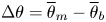 $\Delta {\theta } = \overline { {\theta }}_{m} - \overline { {\theta }}_{b}$.
4. Transient response of the flow field
In this section we describe the transient response of the thermally stratified equilibrium state flow to simultaneous removal of the radiative heat source and imposition of surface cooling. For this purpose we use Case 5 for which  ${\textit {Re}}_{\tau ,0}=540$,
 $Ri_{\tau ,0}=101$, and
 $Ri_{*,0}=52$ (see table 1). The other cases show similar trends. This section is divided into subsections in which we present and discuss: flow visualisations, first- and second-order turbulence statistics, the turbulent kinetic energy and temperature variance budgets, and local stratification length scales and related non-dimensional parameters. In the final subsection we discuss large scale structures that were observed to develop after the destratification process is complete and the flow is evolving toward its new unstably stratified equilibrium state.
4.1. Overview
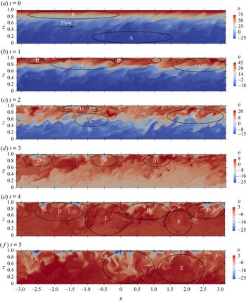
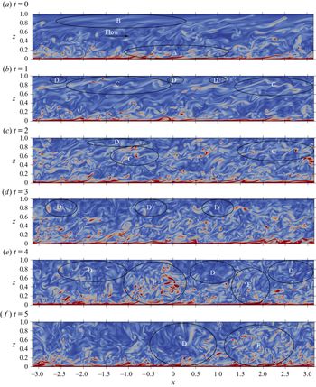
Figures 2 and 3 show the time evolution of the temperature and vorticity fields. Key features discussed below are marked with capital letters in the images. In addition, there are supplementary movies showing the time evolution of the flow field.
Temperature  $\theta$ in an
 $x$-
 $z$ plane during the evolution of the flow for Case 5. Slices were taken through the centre of the domain (
 $y = 0$). The colour scale varies in order to highlight the flow features. Some examples of these features are indicated: A – a weakly stratified turbulent region near the channel bottom; B – a strongly stratified region near the upper boundary in which the flow is close to laminar; C – Kelvin–Helmholtz-like instabilities in the stratified shear layer; D – downwelling thermal plumes; E – near-wall turbulence ejected into the central region by plumes as they reach the channel bottom. Supplementary movies showing the detailed time evolution of the temperature and vorticity fields for each of these time periods are available at https://doi.org/10.1017/jfm.2020.447.

Vorticity magnitude  $\omega$ in an
 $x$-
 $z$ plane during the evolution of the flow for Case 5. Slices were taken through the centre of the domain (
 $y = 0$). The colour scale is the same in all panels, with vorticity range 0 to 300. Some examples of important flow features are indicated: A – a weakly stratified turbulent region near the channel bottom containing hairpin-like vortical structures; B – a strongly stratified region near the upper boundary in which the flow is close to laminar; C – Kelvin–Helmholtz-like instabilities in the stratified shear layer; D – downwelling thermal plumes; E – near-wall turbulence ejected into the central region by plumes as they reach the channel bottom. See also supplementary movies showing the detailed time evolution of the temperature and vorticity fields for each of these time periods.

The initial temperature field in figure 2(a) shows that the channel is weakly stratified close to the bottom wall (A) and becomes progressively more strongly stratified towards the upper boundary (B). The initial state vorticity field shown in figure 3(a) exhibits characteristic features of turbulent channel flow such as hairpin-like vortical structures close to the bottom wall (A). Turbulence is noticeably damped with increasing height and the flow is essentially laminar in the strongly stratified region close to the upper boundary(B).
As the flow evolves the stratification breaks down as a result of the combination of shear from below and cooling from above. In KWAZ, we found that, for the case with no surface cooling, shear instabilities forming in the thermocline play an important role in the destratification process. These instabilities are similar to Kelvin–Helmholtz (K–H) waves, exhibiting the characteristic over-turns in the temperature field and braided cat's eyes in the vorticity field. Similar structures (C) are also clearly visible at a similar location ( $z \approx 0.8$) in the visualisations of the flow with surface cooling at
 $t = 1$. At this time, thermal plumes (D) can also be seen starting to form close to the upper boundary. At
 $t = 2$ the shear instabilities are still apparent but are less prominent, while the thermal plumes have developed into larger structures. At
 $t = 3$ the thermal plumes are a dominant flow feature in the upper half of the channel. By
 $t = 4$ the stable stratification is essentially removed. Large plumes of cooler fluid are seen descending from the surface towards the channel bottom where they interact with the turbulence generated by shear at the channel bottom, ejecting it up into the central region of the channel (E). By this time the flow field is significantly more turbulent than the initial flow. By
 $t = 5$ the downwelling plumes (D) and ejections of wall turbulence (E) have expanded further as the flow approaches a new unstably stratified equilibrium state.
4.2. First- and second-order turbulence statistics
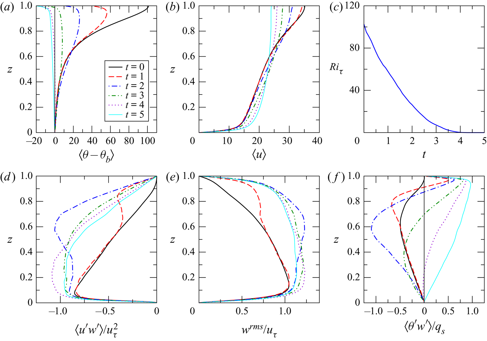
The time evolution of selected first- and second-order turbulence statistics for Case 5 are presented in figure 4. Statistics are shown for the initial equilibrium state,  $t = 0$, and then at five subsequent times,
 $1 \le t \le 5$, during the flow evolution.
Selected turbulence statistics during evolution of the flow for Case 5. Vertical profiles of (a) mean temperature  $\langle \theta \rangle$ relative to the mean temperature at the channel bottom
 $\langle \theta _b \rangle$, (b) mean streamwise velocity
 $\langle u \rangle$, (c) a time series of
 $Ri_{\tau }$, (d–f) vertical profiles of turbulent shear stress
 $\langle u'w' \rangle$, root-mean-squared vertical velocity fluctuation
 $w^{rms} = \langle w'w' \rangle ^{1/2}$ and turbulent heat flux
 $\langle \theta 'w' \rangle$. Here,
 $\langle u'w' \rangle$ and
 $w^{rms}$ are renormalised in terms of the friction velocity
 $\tilde {u}_{\tau }(\tilde {t})$ measured at the time at which the statistic is calculated.
 $\langle \theta 'w' \rangle$ is normalised in terms of the surface cooling flux
 $q_s$.

As discussed in § 2, the friction velocity  $\tilde {u}_{\tau }$ varies during the destratification process. For many statistics it is useful to renormalise in terms of the friction velocity measured at the time at which the statistic is calculated. Thus, in figure 4 for example,
 $\langle u'w' \rangle$, which is normalised in terms of
 $\tilde {u}_{\tau ,0}$, is presented in the form
 $\langle u'w' \rangle / u_{\tau }^2$. Since
 $u_{\tau }(t) = \tilde {u}_{\tau }(\tilde {t})/\tilde {u}_{\tau ,0}$, this has the effect of renormalising
 $\langle u'w' \rangle$ in terms of
 $\tilde {u}_{\tau }(\tilde {t})$. In some cases, such as
 $\langle u \rangle$ and
 $\langle \theta 'w' \rangle$, we chose not to renormalise in this way because the arguments we wish to make are made more clearly without renormalising. We refer the reader to KWAZ for a more detailed discussion of this approach.
The destratification of the channel is clearly apparent in the profiles of mean temperature in figure 4(a). Surface cooling reduces the temperature close to the upper boundary leading to a region of unstable stratification that gradually increases in depth over time. Shear driven mixing from below acts to reduce the temperature gradient in the stably stratified lower part of the channel. By  $t \approx 4$ the initial stable stratification has been removed. This can also be seen from the time series of
 $Ri_{\tau }$ in figure 4(c), which reaches a value of
 $Ri_{\tau }=0$ at approximately
 $t \approx 4$. At this time the destratification process is considered complete. At
 $t = 5$ the flow is unstably stratified over the entire channel height and is evolving toward a new unstably stratified equilibrium state.
The reduction in turbulent mixing in the initial state due to strong stratification close to the upper boundary is apparent in the profile of  $\langle u'w' \rangle$ in figure 4(d), which shows a reduction in magnitude in the near-surface region at
 $t = 0$. As a result the shear stress required to balance the streamwise pressure gradient in this region must be provided predominantly by viscous shear. This leads to the inflected velocity profile seen in figure 4(b), which shows a substantial increase in the mean streamwise velocity close to the upper boundary relative to the final unstably stratified flow.
As the flow evolves there are significant changes to the shear stress profile. At  $t = 1$ there is an enhancement in
 $\langle u'w' \rangle$ from the upper boundary down to
 $z \approx 0.6$ with a peak at
 $z \approx 0.82$. By
 $t = 2$ the enhancement has increased substantially. The peak has descended to
 $z \approx 0.6$ and there is a noticeable increase in
 $\langle u'w' \rangle$ all the way down to
 $z \approx 0.05$, close to the channel bottom. This enhancement is much greater than that seen for the flow with no surface cooling (see KWAZ, figure 6d). From figure 4(e) it can be seen that the enhancement in turbulent shear stress for
 $t = 1$ and
 $t = 2$ corresponds to similar enhancements in the vertical velocity fluctuations. As plumes of cooled fluid descend they increase the vertical velocity fluctuation. Interaction of the downwelling plumes with the streamwise velocity fluctuations leads to augmentation of the turbulent shear stress. This enhancement extends downward as surface plumes penetrate deeper into the channel. The profiles for
 $3 \le t \le 5$ show a region of near constant
 $\langle u'w' \rangle$ for
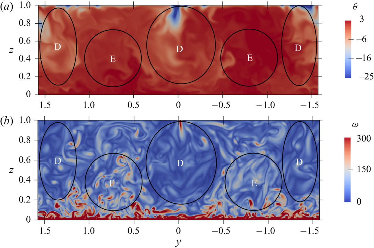
 $0.05 < z < 0.4$ where the plumes interact with the near-wall shear-generated turbulence. In particular, as the plumes approach the bottom of the channel they displace the locally generated turbulence and eject it up into the flow, increasing the turbulent shear stress in the region above the channel bottom. This is seen in the flow visualisations in figure 3 (regions marked E) and more clearly in the flow visualisations showing transverse sections through the flow field in figure 5. Interestingly, at
 $t = 4$ the magnitude of the turbulent shear stress in the region
 $0.05 < z < 0.4$ exceeds the wall shear stress. This imbalance is due to the transient nature of the flow as it is evolving in response to the change in conditions. By
 $t=5$ the flow is evolving toward its new equilibrium state and the balance between wall stress and shear stresses in the near-wall region is restored.
Temperature and vorticity on a transverse section ( $y$-
 $z$ plane) at
 $t = 5$ for Case 5. Slices were taken through the centre of the domain (
 $x=0$) looking upstream. Key flow features are marked: D – downwelling thermal plumes; E – near-wall turbulence ejected into the central region by plumes as they reach the channel bottom.

The turbulent heat flux  $\langle \theta 'w' \rangle$ shown in figure 4(f) also undergoes substantial changes. In the initial heated equilibrium state the net downwards turbulent heat flux (negative
 $\langle \theta 'w' \rangle$) balances the radiative heat source. When the flow switches from internal heating to surface cooling at
 $t = 0$ this balance is disturbed. As the flow destratifies a downwards heat flux continues in the lower, stably stratified region of the channel. Here, as with the turbulent shear stress, descending thermal plumes interact with temperature fluctuations, generating a descending region of strongly enhanced downwards turbulent heat flux at
 $t = 1$ and
 $t = 2$. The heat flux profile differs from the shear stress profile, however, because this region of downwards heat flux is located below a region of upwards heat flux (positive
 $\langle \theta 'w' \rangle$) imposed by the cooling flux applied at the upper boundary. The region of upwards heat flux gradually extends into the channel until by
 $t = 5$ there is an approximately linear profile from
 $\langle \theta 'w' \rangle \approx q_s$ close to the upper boundary to
 $\langle \theta 'w' \rangle = 0$ at the adiabatic channel bottom. This is similar to the heat flux profiles seen in other asymmetric free convection flows (for example, D'Asaro, Winters & Lien Reference D'Asaro, Winters and Lien2002; Zikanov, Slinn & Dhanak Reference Zikanov, Slinn and Dhanak2002).
4.3. Turbulent kinetic energy and temperature variance budgets
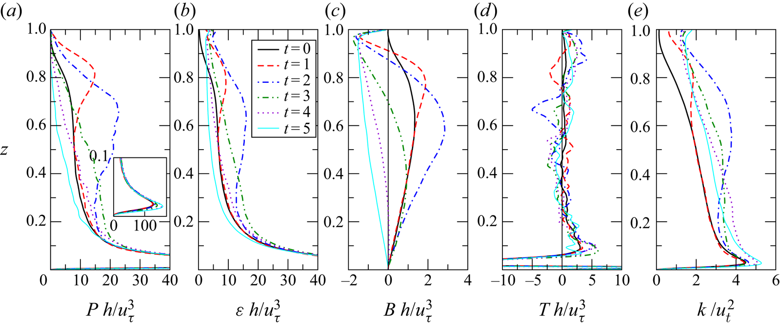
Figure 6 shows the time evolution for Case 5 of the dominant terms in the turbulent kinetic energy budget along with turbulent kinetic energy itself. For this flow, which is homogeneous on  $x$-
 $y$ planes, the turbulent kinetic energy equation can be written as
 \begin{equation} \frac{\partial k}{\partial t} = \frac{\partial}{\partial z} \left[-\frac{1}{2} \langle w'u'_iu'_i \rangle - \langle w'p' \rangle + 2\nu\langle s_{i3}u'_i \rangle \right] - \langle u'w' \rangle \frac{\partial \langle u \rangle}{\partial z} + \gamma \langle \theta'w' \rangle - 2\nu\langle s_{ij} s_{ij} \rangle, \end{equation}
where turbulent kinetic energy 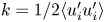 $k = 1/2 \langle u'_iu'_i \rangle$ and
 $s_{ij}$ is the strain rate due to velocity fluctuations given by
 \begin{equation} s_{ij} = \frac{1}{2}\left(\frac{\partial u'_i}{\partial x_j} + \frac{\partial u'_j}{\partial x_i}\right). \end{equation}
The dominant terms in our flow are: shear production  $P=-\langle u'w' \rangle {\partial \langle u \rangle }/{\partial z}$, downwards buoyancy flux
 $B = -\gamma \langle \theta 'w' \rangle$, dissipation rate
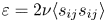 $\varepsilon = 2\nu \langle s_{ij} s_{ij} \rangle$ and transport due to turbulent fluctuations
 $T = -1/2{\partial \langle w'u'_iu'_i \rangle }/{\partial z}$.
Vertical profiles of turbulent kinetic energy budget terms for Case 5: (a) shear production, (b) dissipation rate, (c) downwards buoyancy flux, (d) turbulent transport and (e) turbulent kinetic energy. All terms are renormalised with respect to the friction velocity  $\tilde {u}_{\tau }(\tilde {t})$ measured at the time at which the statistic is calculated.

During the first half of the destratification process (up to  $t = 2$) there is substantial enhancement of
 $P$,
 $B$ and
 $\varepsilon$ in the upper two thirds of the channel, with peaks at
 $z \approx 0.82$ at
 $t = 1$ that descend to
 $z \approx 0.6$ to 0.7 at
 $t = 2$. The peaks for
 $B$ are at a slightly lower height than those for
 $P$ and
 $\varepsilon$ due to the region of negative
 $B$ (upwards buoyancy flux) above. In the initial equilibrium state, as can be seen in the mean velocity profile in figure 4(b), there is significant shear present between
 $z=0.5$ and 0.9. As described in KWAZ, removal of the heat source allows this region to destabilise, leading to the formation of Kelvin–Helmholtz-like instabilities. For the case without surface cooling, these instabilities were found to be associated with an increase in turbulent mixing, leading to increased
 $P$,
 $B$ and
 $\varepsilon$ in this region. For the current case of flow with surface cooling similar K–H-like instabilities are also present, as is evident from the flow field visualisations (regions marked C in figures 2 and 3). In this case, however, the increases in
 $P$,
 $B$ and
 $\varepsilon$ are much more substantial. This difference can be explained by the fact that, as seen above, when surface cooling is present the thermal plumes generate vertical velocity fluctuations that cause substantial enhancements in the turbulent shear stress and heat flux, which in turn contribute to the shear production and downwards buoyancy flux. Thus, for the flow with surface cooling, enhanced mixing is due to a combination of K–H-like shear instabilities and downwelling thermal plumes. The interactions between these flow features is most clearly seen in the supplementary movies.
Enhancement of shear production by thermal plumes through enhancement of the turbulent shear stress occurs only while the vertical mean velocity gradient is maintained. The reduction in  $P$ for
 $z > 0.8$ at
 $t = 2$ relative to
 $t = 1$ is due to a reduction in the mean velocity gradient in this region (see figure 4b) as a result of turbulent mixing by the evolving convective instabilities. As the plumes penetrate deeper the region over which shear production is attenuated extends downwards. In the near-wall region (
 $z < 0.1$), however, (see inset in figure 6a) shear production increases in the later stages of the flow evolution (
 $t > 3$) as the plumes interact strongly with wall turbulence and shear.
The imposition of surface cooling to a system that is initially stably stratified leads to a profile for the buoyancy flux,  $B$, that changes sign within the channel. In the upper part of the channel the buoyancy flux is upwards (
 $B < 0$) indicating net transfer of energy from potential energy to turbulent kinetic energy. In the lower part of the channel the buoyancy flux is downwards (
 $B > 0$), indicating net transfer of energy from turbulent kinetic energy to potential energy.
Profiles of dissipation  $\varepsilon$ and
 $k$ follow similar trends to shear production. Globally, there is an imbalance between
 $P$,
 $B$ and
 $\varepsilon$ so that by the end of the flow evolution there is an increase in turbulent kinetic energy
 $k$ in the channel.
The profiles of turbulent transport  $T$ are quite noisy; however, the profiles at
 $t=1$ and
 $t=2$ indicate regions of negative
 $T$ around
 $z \approx 0.8$ and
 $z \approx 0.7$ respectively at these times, which may represent downwards transport of turbulent kinetic energy by descending thermal plumes. At
 $t = 2$ there is also a region of positive
 $T$ around
 $z \approx 0.9$ which indicates transport of turbulence from the more energetic central region of the channel up into the now unstably stratified region close to the top of the channel.
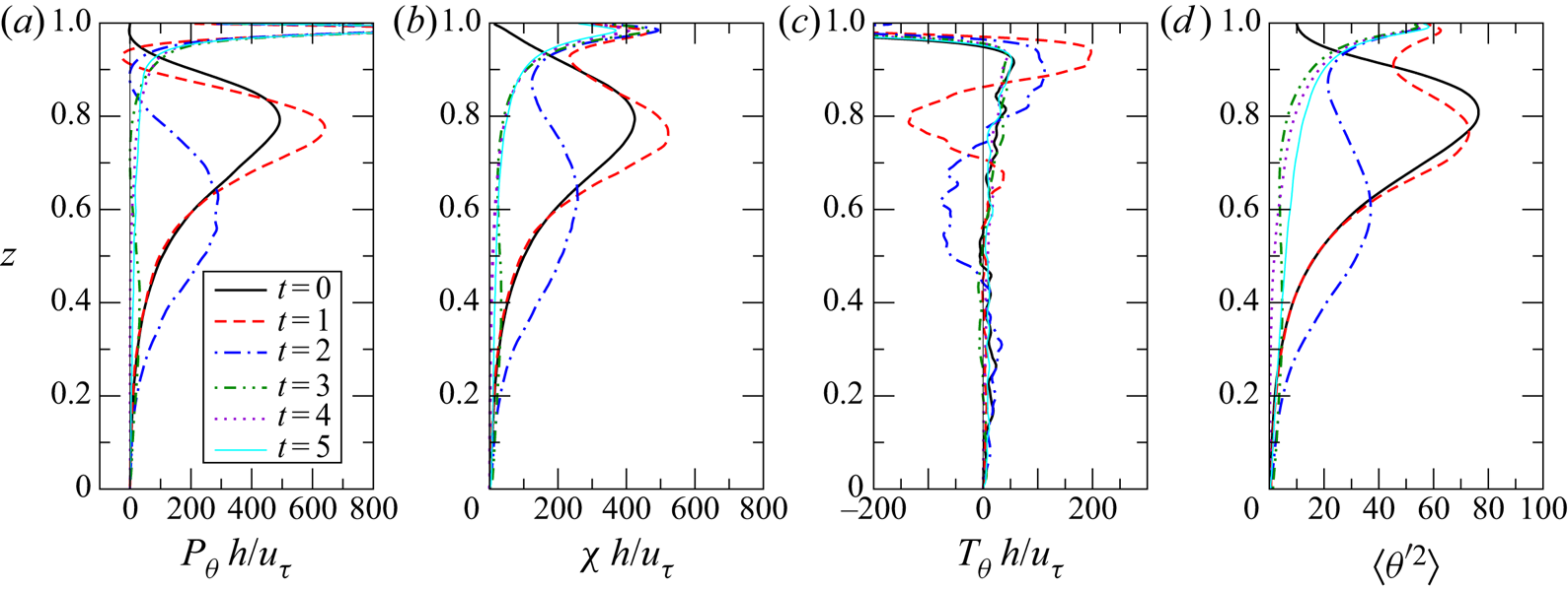
Figure 7 shows the transient response of dominant terms in the transport equation for temperature variance  $\langle \theta '^2 \rangle$. For our flow the temperature variance equation can be written as
 \begin{equation} \frac{\partial \langle \theta'^2 \rangle}{\partial t} = \frac{\partial}{\partial z} \left[ -\langle w'\theta'^2 \rangle + \kappa\frac{\partial \langle \theta'^2 \rangle}{\partial z} \right]- 2\langle \theta'w' \rangle \frac{\partial \langle \theta \rangle}{\partial z} - 2\kappa\left\langle\frac{\partial \theta'}{\partial x_j}\frac{\partial \theta'}{\partial x_j}\right\rangle. \end{equation}
The dominant terms are production  $P_{\theta }=-2\langle \theta 'w' \rangle {\partial \langle \theta \rangle }/{\partial z}$, turbulent transport
 $T_{\theta } = -{\partial \langle w'\theta '^2 \rangle }/{\partial z}$ and dissipation rate
 $\chi = 2\kappa \langle (\partial \theta '/\partial x_j)^2 \rangle$.
Vertical profiles of temperature variance budget terms for Case 5: (a) production, (b) dissipation rate, (c) turbulent transport and (d) temperature variance. All terms are renormalised with respect to the friction velocity  $\tilde {u}_{\tau }(\tilde {t})$ measured at the time at which the statistic is calculated.

In the initial flow, temperature variance is produced predominantly in a region centred around the thermocline at  $z \approx 0.8$, where both the vertical temperature gradient and turbulent heat flux are high (see figure 4). As a result,
 $P_{\theta }$,
 $\chi$ and
 $\langle \theta '^2 \rangle$ have a similar distribution.
Imposition of surface cooling adds a new source of temperature variance at the upper boundary, leading to a rapid increase in  $P_{\theta }$ just below the surface. This, combined with transition of the near-surface region to turbulent flow, leads to a substantial increase in
 $\langle \theta '^2 \rangle$ close to the upper boundary at
 $t = 1$. The increased intensity of turbulence around
 $z = 0.8$ also leads to an increase in
 $P_{\theta }$ in this region at
 $t = 1$; however, this is balanced by an increase in
 $\chi$ and transport
 $T_{\theta }$ out of this region (
 $0.7 < z < 0.85$) into the region above (
 $0.85 < z < 0.95$), so that
 $\langle \theta '^2 \rangle$ remains relatively constant for
 $z < 0.8$ at this time, while it increases for
 $z > 0.9$. In the region
 $0.9 < z < 0.95$ the temperature gradient is close to zero so
 $P_{\theta }$ becomes very small, and in fact becomes negative, indicating a small region of counter-gradient turbulent heat flux at
 $t=1$.
Similar dynamics is in play at  $t = 2$; however, the thermal plumes have now penetrated deeper into the channel. For
 $t \ge 3$ the mean temperature gradient in regions below
 $z = 0.9$ is very small and production of temperature variance
 $P_{\theta }$ is confined predominantly to the region close to the upper boundary. The profiles of
 $T_{\theta }$ show that downwelling plumes transport temperature fluctuations out of this region into the lower regions leading to a temperature variance profile that gradually decreases with increasing depth in the late stages of the flow evolution.
4.4. Local flow parameters and length scales
In this section we present vertical profiles of gradient Richardson number  $Ri$, shear Reynolds number
 $Re_S$, buoyancy Reynolds number
 ${\textit {Re}}_b$ and related turbulence length scales, the Kolmogorov
 $\eta$, Corrsin
 $l_C$ and Ozmidov
 $l_O$ length scales. These parameters and length scales can be used to characterise local flow conditions in stratified turbulence (see for example, Chung & Matheou Reference Chung and Matheou2012). All parameters and length scales are non-dimensionalised in terms of
 $\tilde {h}$,
 $\tilde {u}_{\tau ,0}$ and
 $\tilde {\Theta }_{N}$ (see (2.15)).
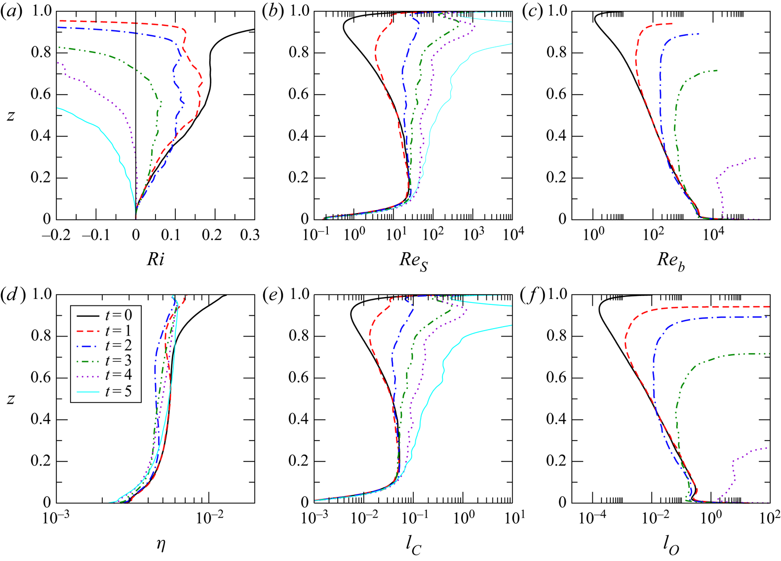
Figure 8(a) shows the time evolution of vertical profiles of the gradient Richardson number. The gradient Richardson number  $Ri = N^2/S^2$ gives an indication of the stability of the flow with respect to density stratification characterised by buoyancy frequency
 $N = (\gamma \, \partial \langle \theta \rangle / \partial z)^{1/2}$, and velocity shear
 $S = \partial \langle u \rangle / \partial z$. Alternatively,
 $Ri$ can be written in terms of the ratio between the Corrsin
 $l_C$ and Ozmidov
 $l_O$ length scales,
 $Ri \equiv ({l_C}/{l_O})^{4/3}$, and hence can be interpreted as the degree of separation between scales above which turbulence is strongly affected by shear and buoyancy (Chung & Matheou Reference Chung and Matheou2012).
Selected non-dimensional parameters and length scales characterising stratified turbulence for Case 5: (a) the gradient Richardson number  $Ri = ({l_C}/{l_O})^{4/3}$, (b) the shear Reynolds number
 $Re_S = ({l_C}/{\eta })^{4/3}$, (c) the local buoyancy Reynolds number
 ${\textit {Re}}_b = ({l_O}/{\eta })^{4/3}$, (d) the Kolmogorov scale
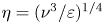 $\eta =({\nu ^3}/{\varepsilon })^{1/4}$, (e) the Corrsin scale
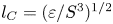 $l_C = ({\varepsilon }/{S^3})^{1/2}$ and (f) the Ozmidov scale
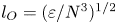 $l_O = ({\varepsilon }/{N^3})^{1/2}$.

The profile for  $Ri$ in the initial equilibrium state (figure 8a) shows three distinct regimes spanning three regions across the channel. For
 $0 < z < 0.5$,
 $Ri$ increases from
 $Ri \approx 0$ at the channel bottom to a value of
 $Ri \approx 0.18$. In this region
 $l_C$ (figure 8e) is relatively constant except in the region very close to the channel bottom, while
 $l_O$ (figure 8f) decreases with height due to increasing stratification. For
 $0.5 < z < 0.75$,
 $l_C$ and
 $l_O$ both decrease at approximately the same rate with increasing height, so that
 $Ri$ is approximately constant at what appears to be a critical value of
 $Ri_c \approx 0.18$. Comparable values of
 $Ri_c$ have been reported for a range of stratified shear flows including the following: stratified channel flow (Garcia-Villalba & del Alamo Reference Garcia-Villalba and del Alamo2011), stationary homogeneous stratified sheared turbulence (Shih et al. Reference Shih, Koseff, Ferziger and Rehmann2000; Chung & Matheou Reference Chung and Matheou2012), stratified plane Couette flow (Zhou et al. Reference Zhou, Taylor and Caulfield2017) and the stably stratified atmospheric boundary (Basu & Porté-Agel Reference Basu and Porté-Agel2006). For
 $0.75 < z < 1$,
 $l_O$ decreases more rapidly than
 $l_C$, so that
 $Ri$ increases significantly. As discussed above with respect to the flow visualisations in figures 2(a) and 3(a), above this height turbulence is intermittent and the flow becomes essentially laminar close to the upper boundary.
As the flow evolves, the profiles of  $Ri$ show an expanding region of negative
 $Ri$ close to the upper boundary, which represents unstable stratification resulting from the formation of convective plumes due to the surface cooling. At any time, the point at which
 $Ri$ changes sign delineates the boundary between the unstably and stably stratified regions of the flow. When no surface cooling is present, KWAZ found that the value of
 $Ri$ in the central region of the flow remains constant at
 $Ri \approx 0.18$ until the late stages of the flow evolution. In contrast, the profiles shown here for the case with surface cooling show a progressive reduction in
 $Ri$ in the central region of the channel, which can be attributed to the effect of thermal plumes penetrating into this region. The extra turbulent mixing reduces both temperature and velocity gradient; however, the fact that
 $Ri$ decreases indicates that the temperature gradient is reduced more rapidly.
Figure 8(b) shows the time evolution of vertical profiles of the shear Reynolds number 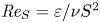 $\textit {Re}_S = {\varepsilon }/{\nu S^2}$, which can also be written as a function of the ratio of Corrsin and Kolmogorov length scales,
 $\textit {Re}_S = ({l_C}/{\eta })^{4/3}$, and hence gives an indication of the extent of the inertial subrange (Chung & Matheou Reference Chung and Matheou2012).
In the initial equilibrium state,  $\textit {Re}_S$ also shows multiple flow regimes across the height of the channel resulting from changes in
 $l_C$ and
 $\eta$. For
 $0 < z < 0.1$, shear at the channel bottom drives
 $l_C$ and
 $\textit {Re}_S$ toward zero and viscous effects dominate. In the weakly stratified turbulent boundary layer,
 $0.1 < z < 0.5$,
 $\textit {Re}_S$ is in the range 10–20, indicating approximately an order of magnitude separation between
 $\eta$ and
 $l_C$, both of which are approximately constant in this region. For
 $0.5 < z < 0.8$,
 $\eta$ remains approximately constant while both
 $l_C$ and
 $\textit {Re}_S$ decrease as a result of increasing shear (see velocity profile in figures 4a and 4b). In the region
 $0.8 < z < 0.95$,
 $\eta$ increases as significant damping of turbulence by stratification decreases viscous turbulence dissipation
 $\varepsilon$. Meanwhile
 $l_C$ continues to decrease, so that
 $Re_S$ drops below 1. Very close to the upper boundary,
 $0.95 < z < 1$, shear decreases again leading to an increase in
 $l_C$ and
 $Re_S$.
As the flow evolves, the main change seen is a significant increase in  $Re_S$ due to a reduction in shear and hence an increase in
 $l_C$. This process starts in the region close to the upper surface as thermal plumes break down the stably stratified shear layer, replacing it with a strongly mixed, convectively unstable region in which shear is close to zero. The region of increased
 $l_C$ and
 $Re_S$ expands downwards over time as the thermal plumes penetrate further into the channel.
Figure 8(c) shows the time evolution of vertical profiles of the local buoyancy Reynolds number 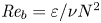 ${\textit {Re}}_b = {\varepsilon }/{\nu N^2}$, which can also be written as a function of the ratio of Ozmidov and Kolmogorov scales
 ${\textit {Re}}_b = ({l_O}/{\eta })^{4/3}$, giving a measure of the degree of separation between the scale above which fluid motion is influenced by stable buoyancy stratification and the smallest scales of motion (Brethouwer et al. Reference Brethouwer, Billant, Lindborg and Chomaz2007).
The buoyancy Reynolds number has received considerable attention in the literature due to its importance in geophysical measurements and modelling, where it is used in parameterisations for eddy viscosity (for example, Osborn Reference Osborn1980; Shih et al. Reference Shih, Koseff, Ivey and Ferziger2005), and mixing efficiency (for example, Mater & Venayagamoorthy Reference Mater and Venayagamoorthy2014; Walter et al. Reference Walter, Squibb, Woodson, Koseff and Monismith2014; Scotti & White Reference Scotti and White2016; Ivey et al. Reference Ivey, Bluteau and Jones2018). In KWAZ we give an in-depth discussion and comparison of a number of these parameterisations with results obtained in our stratified channel flow simulations, and show that parameterisations developed for the ocean and stably stratified atmospheric boundary layer also accurately predict turbulence properties in the central region of stably stratified open-channel flow. In the following, we focus primarily on features resulting from the introduction of surface cooling.
Shih et al. (Reference Shih, Koseff, Ivey and Ferziger2005) define three regimes for  ${\textit {Re}}_b$ in stably stratified turbulent shear flows: a diffusive regime for
 ${\textit {Re}}_b < 7$ in which turbulence is strongly damped and viscous effects dominate, an intermediate regime
 $7 < {\textit {Re}}_b < 100$ in which turbulence is energetic but significantly affected by stratification, and an energetic regime,
 ${\textit {Re}}_b > 100$, in which the effects of stratification become progressively weaker as
 ${\textit {Re}}_b$ increases. In the initial equilibrium state for our simulations
 ${\textit {Re}}_b$ covers all three regions described above, with the energetic regime seen for
 $0 < z < 0.4$, the intermediate regime for
 $0.4 < z < 0.8$, and the diffusive regime for
 $0.8 < z < 1$. Comparison with
 $l_O$ in panel (f) shows that this sweep of regimes is due primarily to the three orders of magnitude decrease in
 $l_O$, which in turn is due primarily to the fact that stratification in our case is driven by progressive absorption of radiation from above and hence is strongest close to the upper boundary. Dissipation decreases with height but this decrease is relatively small for
 $z > 0.15$.
After the application of surface cooling, the profiles of  ${\textit {Re}}_b$ show three distinct regions: an upper region in which
 $\textit {Re}_b$ becomes very large and is then undefined, a central region in which
 ${\textit {Re}}_b$ is approximately constant with height and a lower region in which
 $Re_b$ remains close to its initial equilibrium state profile. The upper region corresponds to the unstably stratified convective region where
 $l_O$ and
 ${\textit {Re}}_b$ are undefined. The central region is stably stratified in a horizontally averaged sense, but convective plumes penetrate into this region providing extra mixing and leading to relatively uniform stratification conditions across this region. The lower region represents the region that is only weakly affected by surface convection.
Interestingly, at  $t = 5$ there is a region close to the bottom boundary (
 $0 < z < 0.3$) in which
 $l_O > 1$. Since
 $l_O$ has been non-dimensionalised in terms of
 $\tilde {h}$, this indicates that the distance a parcel of fluid must travel in order to be significantly affected by stable stratification in this region is greater than the channel height. Since this is not possible,
 $l_O > 1$ indicates that, while the background stratification is still stable in this region, it is so weak that flow conditions are effectively neutral. By
 $t = 6$ this region has become unstable and
 $l_O$ is undefined throughout the channel.
4.5. Large scale flow structures in the destratified flow
In this section we describe large scale flow structures that are observed to form after all of the background stratification has been removed and the flow is evolving toward a new unstably stratified equilibrium state.
The time at which the flow becomes fully destratified, in the sense that all background stratification is removed, corresponds to a fundamental regime change. At this time the difference between the maximum horizontally averaged temperature in the channel and the horizontally averaged temperature at the channel bottom reaches zero, that is  $\Delta {\theta } = \overline { {\theta }}_m - \overline { {\theta }}_b = 0$, and remains at this value since
 $\overline { {\theta }}_m = \overline { {\theta }}_b$. As a result, the two Richardson numbers,
 $Ri_{\tau }$ and
 $Ri_*$ also become fixed equal to
 $0$, and hence no longer act as governing parameters. The flow is now evolving toward a new equilibrium flow state, namely, unstably stratified turbulent open-channel flow. For Case 5 this occurs at a time of
 $t\approx 4$ as seen in figure 4(c).
This new equilibrium state has been studied by Walker et al. (Reference Walker, Tejada-Martínez, Martinat and Grosch2014), who suggest that it is governed by the parameters  ${\textit {Re}}_{\tau }$,
 $Pr$ and a Rayleigh number
 $Ra_{\tau }$, which they define as
 \begin{equation} Ra_{\tau} = \frac{\tilde{\beta} \tilde{g} \tilde{h}^2 \tilde{q}_s}{\tilde{\rho}_b \tilde{c}_p \tilde{\kappa} \tilde{u}_{\tau}^2}. \end{equation}
For Case 5, at  $t = 5$,
 $u_{\tau } \approx 1.2$ so
 $Ra_{\tau } \approx 700$. This is somewhat lower than the value used by Walker et al. (Reference Walker, Tejada-Martínez, Martinat and Grosch2014) (
 $Ra_{\tau } \approx 5000$). Walker et al. (Reference Walker, Tejada-Martínez, Martinat and Grosch2014) give a detailed discussion of the turbulent structure of the flow field for statistically steady open-channel flow subject to surface cooling. This material will not be repeated here. Instead we focus on the formation of large scale flow structures.
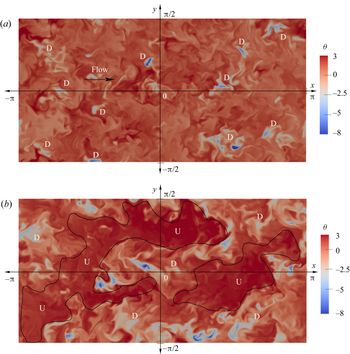
For our flow, large scale structures were observed to start forming after the regime change noted above, that is, between  $t=4$ and
 $t=5$ for Case 5. Figure 9 shows visualisations of the temperature field at these times on a horizontal section at the channel mid-depth (
 $z=0.5$). At
 $t=4$ isolated intense downwelling thermal plumes (marked D) can be seen penetrating the central plane; however, the remainder of the temperature field is relatively homogeneous. By
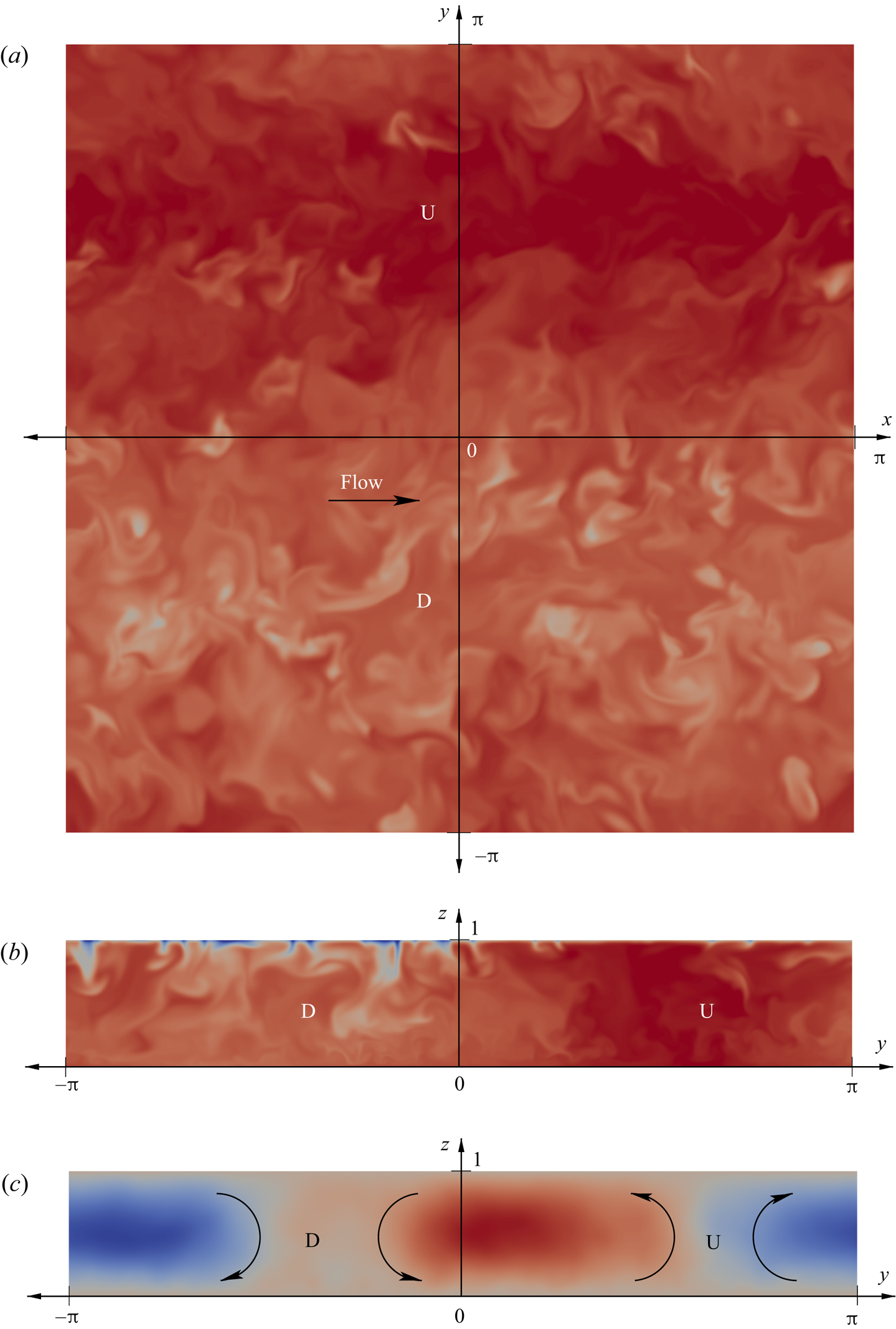
 $t=5$, large scale structures, elongated primarily in the streamwise direction, are apparent. The low temperature regions correspond to downwelling (D) of cooler fluid from the upper boundary, while the higher temperature regions correspond to upwelling (U) of warmer fluid from below. This can be seen clearly by comparison with the transverse sections in figure 5. Each structure (an upwelling/downwelling pair) has a lateral dimension of approximately half the domain width.
Temperature at  $t = 4$ and 5 for Case 5 on a horizontal plane at the channel mid-depth (
 $z=0.5$). (a) At
 $t = 4$, isolated cooler downwelling thermal plumes (D) are visible penetrating this layer. (b) At
 $t = 5$, large coherent regions of upwelling warmer fluid (U) and downwelling cooler fluid (D) are apparent.

Inspection of flow visualisations at later times showed that these structures grow and become more coherent and elongated until, by approximately  $t=6$, they eventually reach a width approximately equal to the domain width, after which they were restricted from further growth by the domain. Thus it appears that, as the flow starts evolving towards its final unstably stratified equilibrium state, the domain size also starts having an effect on the lateral dimension of these large scale structures.
This was confirmed through observation of the results for Case 9, which used the wider domain of  $L_y = 2 \pi h$. On the larger domain, the structures eventually reach a size approximately equal to the domain width. This can be seen in the visualisations of horizontal and transverse sections through the temperature field for Case 9 at
 $t=10$ shown in figures 10(a) and 10(b). The flow is clearly divided in the lateral dimension into a single pair of upwelling and downwelling zones. This is made more clear by the transverse section of the streamwise-averaged streamfunction in figure 10(c), which shows clear clockwise and anticlockwise circulations centred on the vertical boundaries between these two zones.
Temperature and streamfunction at  $t = 10$ for Case 9. (a) Shows temperature on a horizontal
 $x\hbox{--}y$ plane at
 $z=0.5$. (b and c) Transverse sections at
 $x=0$ looking upstream. Temperature range:
 $-30$ to 5. Streamfunction range:
 $-0.6$ to 0.5. U indicates upwelling flow, while D indicates downwelling flow.

Similar large scale structures were observed by Walker et al. (Reference Walker, Tejada-Martínez, Martinat and Grosch2014), who refer to them as ‘convective supercells’. They found that the supercells in their simulations have a width four times the channel depth. Given that their domain width was  $L_y = 4 \pi h/3$, this is also approximately equal to their domain width.
Thus it appears that, for the steady-state unstably stratified channel flow, domain widths up to  $2\pi h$ may be placing a constraint on the size of these supercells.
This effect of domain size is confined to the stages of the flow evolution that occur after the flow has fully destratified – that is, after the time period for which  $\Delta {\theta } > 0$, which is the subject of the discussions presented in the previous subsections, and in the scaling analysis presented below. For the time period over which
 $\Delta {\theta } > 0$, the results for Case 9, which uses the larger domain, were found to be very similar to the results for Case 6, which has the identical parameter settings on the standard size domain, indicating that domain size has negligible effect on these earlier stages of the flow evolution.
5. Scaling analysis
5.1. Time scales
As shown above, the destratification process involves an interplay between three dominant characteristics of the flow: turbulent fluid motion generated by bottom friction, turbulent fluid motion generated by surface cooling, and damping of these motions by the stable background stratification. As such, it is useful to define characteristic time scales associated with these three dominant processes, namely a friction time scale  $\tilde {t}_{\tau }$, convection time scale
 $\tilde {t}_*$ and buoyancy time scale
 $\tilde {t}_N$:
 \begin{equation} \tilde{t}_{\tau}(\tilde{t}) = \frac{\tilde{h}}{\tilde{u}_{\tau}(\tilde{t})},\quad \tilde{t}_* = \frac{\tilde{h}}{\tilde{w}_*}, \quad \tilde{t}_N(\tilde{t}) = \left(\frac{\tilde{\beta} \tilde{g} \Delta\tilde{\theta}(\tilde{t})}{\tilde{h}}\right)^{-1/2}. \end{equation}
Written in terms of our non-dimensionalisation scheme (where  $t = \tilde {t}/\tilde {t}_{\tau ,0}$ with
 $\tilde {t}_{\tau ,0} = \tilde {h}/\tilde {u}_{\tau ,0}$), the equivalent dimensionless time scales are
 \begin{equation} {t}_{\tau}({t}) = \frac{{h}}{{u}_{\tau}({t})},\quad {t}_* = \frac{{h}}{{w}_*}, \quad {t}_N({t}) = \left(\frac{\gamma \Delta{\theta}({t})}{{h}}\right)^{-1/2}. \end{equation}
In our flow the friction time scale  $ {t}_{\tau }$ varies with time due to the time variation of
 $u_{\tau }$, while the buoyancy time scale
 $ {t}_N$ varies due to the change in the mean temperature gradient. On the other hand, the surface cooling flux remains constant, so the convection time scale
 $ {t}_*$ is constant.
The two Richardson numbers defined in (2.19) can be reformulated as ratios of these three time scales,
 \begin{equation} Ri_{\tau}(t) = \left(\frac{\tilde{t}_{\tau}}{\tilde{t}_N}\right)^2 = \left(\frac{{t}_{\tau}}{{t}_N}\right)^2\quad \text{and} \quad Ri_*(t) = \left(\frac{\tilde{t}_*}{\tilde{t}_N}\right)^2 = \left(\frac{{t}_*}{{t}_N}\right)^2, \end{equation}
and hence can be interpreted as representing ratios between the time scales of shear- and convection-generated fluid motions to the time scale associated with the deceleration of fluid parcels by the background stratification.
The convection velocity  $ {w}_*$ and time scale
 $ {t}_*$ given above use the channel height
 $h$ as their length scale. This approach has the advantage that it allows the development of the relatively simple scaling formulas presented below, and, in particular the formula for destratification time presented in § 5.3. The assumption implicit here is that the effect of the plumes is felt throughout the depth of the channel. This assumption is reasonable during later stages of the destratification process, but over-estimates
 $ {w}_*$ during the initial stages when plumes are confined to the region close to the surface.
An alternative approach is to use a length scale based on some measure of the penetration depth of the plumes in a manner analogous to the original scaling of Deardorff (Reference Deardorff1970). In this case,  $ {w}_*$ and
 $ {t}_*$ vary with time as the plumes penetrate progressively further into the channel. An approach similar to this was adopted by Ulloa et al. (Reference Ulloa, Winters, Wüest and Bouffard2019) in their recent analysis of penetrative convection in ice-covered lakes. The resultant scaling is, however, significantly more complex because it requires knowledge or prediction of the time evolution of the penetration depth of the plumes. The development of an alternative scaling based on this more complex approach is the subject of ongoing work by the authors.
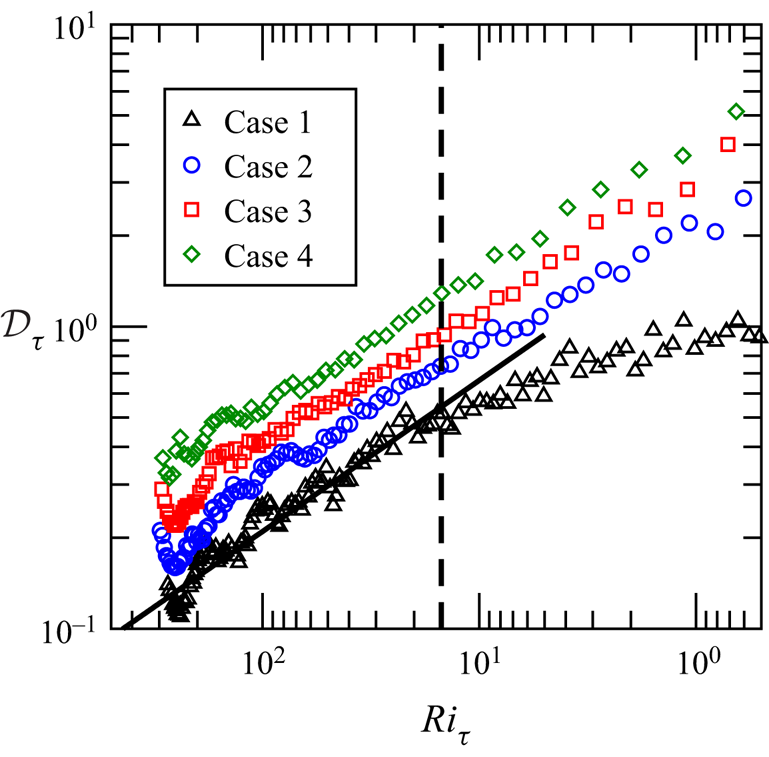
5.2. Destratification rate
In order to determine a scaling for the destratification rate, we first define a destratification rate,  ${\mathcal {D}}_{\tau }$, non-dimensionalised in terms of the friction time scale and the temperature difference at that time:
 \begin{equation} {\mathcal{D}}_{\tau} = -\frac{\textrm{d}\Delta \tilde{\theta}}{\textrm{d} \tilde{t}}\frac{\tilde{t}_{\tau}}{\Delta \tilde{\theta}} = -\frac{\textrm{d}\Delta {\theta}}{\textrm{d} {t}}\frac{{t}_{\tau}}{\Delta {\theta}}. \end{equation}
This is equivalent to the destratification rate  ${\mathcal {D}}$ defined in KWAZ for the case without surface cooling. In the current paper we will non-dimensionalise the destratification rate in terms of the three time scales
 $ {t}_{\tau }$,
 $ {t}_*$ and
 $ {t}_N$ defined above and distinguish between these by using subscripts
 $_{\tau }$,
 $_*$ and
 $_N$ appended to
 ${\mathcal {D}}$. We will also divide destratification rate into components attributed to the two main forcings – bottom shear and surface cooling. These will be indicated by superscripts
 $^s$ and
 $^c$, respectively. No superscript indicates total destratification rate. These symbols are defined explicitly in the table of symbols contained in table 3. Figure 11 shows
 ${\mathcal {D}}_{\tau }$ plotted as a function of
 $Ri_{\tau }$ for Cases 1–4, for which the surface cooling flux
 $q_s$ varies from 0 to 2.67 and
 $ {w}_*$ from 0 to 1.75.
 $Ri_{\tau }$ decreases as the flow evolves, so flow evolution proceeds from left to right. As
 $Ri_{\tau }$ decreases, the stability of the flow decreases, and the destratification rate increases. As expected, destratification rate also increases with increasing
 $q_s$.
Value of  ${\mathcal {D}}_{\tau }$ as a function of
 $Ri_{\tau }$ for Cases 1–4. The solid line is the model for destratification rate attributed to shear,
 ${\mathcal {D}}_{\tau }^{s,{\textrm {mod}}} = C_1 Ri_{\tau }^{-1/2}$, with
 $C_1 = 2.1$. The dashed line indicates the lower limit of validity of this model,
 $Ri_{\tau } = 15$.

In KWAZ we found that, for the flow without surface cooling, the destratification rate can be modelled using the power law relationship
 \begin{equation} {\mathcal{D}}_{\tau}^{s,{\textrm{mod}}} = C_1 Ri_{\tau}^{-1/2} \quad \text{for}\ Ri_{\tau} > 15, \end{equation}
where  $C_1 = 2.1$. In Case 1 (no surface cooling) destratification is driven only by turbulence generated by shear, so this case isolates the effect of bottom shear on destratification rate and
 ${\mathcal {D}}_{\tau } = {\mathcal {D}}_{\tau }^s$.
The relationship (5.5) is shown in figure 11. For Case 1 ( $q_s = 0$) the data follow (5.5) for
 $Ri_{\tau } > 15$. For weak stratification, where
 $Ri_{\tau } < 15$, the exponent decreases and
 ${\mathcal {D}}_{\tau }^s$ approaches an asymptotic value of
 ${\mathcal {D}}_{\tau }^s \approx 1.1$ for neutral conditions.
In riverine flows in which thermal stratification is an issue, the friction Richardson number of the thermally stratified state is typically of order  $Ri_{\tau } = \textit {O}(1000)$ (see field measurement data in Bormans & Webster Reference Bormans and Webster1998; Sherman et al. Reference Sherman, Webster, Jones and Oliver1998; Mitrovic et al. Reference Mitrovic, Oliver, Rees, Bowling and Buckney2003). In this context the weakly stratified flow regime,
 $Ri_{\tau } < 15$, corresponds to a degree of stratification that is less than
 $\textit {O}(1\,\%)$ of its initial value and hence is negligible when determining quantities such as the time taken for effective destratification of the flow. In the following analysis we focus on the flow regime in which
 $Ri_{\tau } > 15$ and (5.5) is valid.
When  $q_s > 0$, surface cooling provides a second driver for destratification. In order to isolate this second process we subtract the destratification due to bottom shear modelled by (5.5) from the total destratification rate:
 \begin{equation} {\mathcal{D}}_{\tau}^c = {\mathcal{D}}_{\tau} - {\mathcal{D}}_{\tau}^{s,{\textrm{mod}}} = -\frac{\textrm{d}\Delta {\theta}}{\textrm{d} {t}}\frac{{t}_{\tau}}{\Delta {\theta}} - C_1 Ri_{\tau}^{-1/2}. \end{equation}
Here,  ${\mathcal {D}}_{\tau }^c$ denotes destratification rate due to surface cooling non-dimensionalised in terms of the friction time scale
 $ {t}_{\tau }$. Implied here is an assumption that coupling between processes associated with destratification by shear and convection is linear.
Since destratification due to surface cooling is expected to scale with the convection time scale  $ {t}_*$ rather than the friction time scale, we re-scale
 ${\mathcal {D}}_{\tau }^c$ in terms of
 $ {t}_*$, to give the destratification rate due to cooling non-dimensionalised in terms of convection time scale:
 \begin{equation} {\mathcal{D}}_*^c = ({\mathcal{D}}_{\tau} - {\mathcal{D}}_{\tau}^{s,{\textrm{mod}}}) \frac{{t}_*}{{t}_{\tau}} = -\frac{\textrm{d}\Delta {\theta}}{\textrm{d} {t}}\frac{{t}_*}{\Delta {\theta}} - C_1\frac{{t}_*}{{t}_{\tau}} Ri_{\tau}^{-1/2}. \end{equation}
This can be written more concisely as
 \begin{equation} {\mathcal{D}}_*^c = {\mathcal{D}}_* - {\mathcal{D}}_*^{s,{\textrm{mod}}}, \end{equation}
where  ${\mathcal {D}}_*$ is the total destratification rate non-dimensionalised in terms of the convection time scale,
 \begin{equation} {\mathcal{D}}_* = -\frac{\textrm{d}\Delta {\theta}}{\textrm{d} {t}}\frac{{t}_*}{\Delta {\theta}}, \end{equation}
and  ${\mathcal {D}}_*^{s,{\textrm {mod}}}$ is the modelled destratification rate due to bottom shear rescaled in terms of the convection time scale,
 \begin{equation} {\mathcal{D}}_*^{s,{\textrm{mod}}} = C_1\frac{{t}_*}{{t}_{\tau}} Ri_{\tau}^{-1/2}. \end{equation}
By analogy with  ${\mathcal {D}}_{\tau } = f(Ri_{\tau })$ and the scaling relation (1.1) of Deardorff et al. (Reference Deardorff, Willis and Stockton1980), we expect the destratification rate associated with surface cooling
 ${\mathcal {D}}_*^c$ to be a function of the convection Richardson number
 $Ri_*$. Figure 12(a) shows
 ${\mathcal {D}}_*^c$ plotted as a function of
 $Ri_*$ for Cases 2–4, for which
 $q_s$ increases from 0.53 to 2.67 and
 $ {w}_*$ from 1.02 to 1.75. The data for different surface heat fluxes collapse to a relationship
 \begin{equation} {\mathcal{D}}_*^{c,{\textrm{mod}}} = C_2Ri_*^{-1/2}, \end{equation}
where  $C_2 = 1.2$. There is some scatter in the data especially at high
 $Ri_*$. Inspection of the data for individual cases shows an initial oscillatory variation in
 ${\mathcal {D}}_*^c$ around (5.11). This occurs during the early relaxation period as the flow responds to the sudden change in conditions from radiative heating to surface cooling and the region close to the upper boundary undergoes a transition from laminar to turbulent flow. This can be clearly seen in figure 12(b) which shows the data for Case 3 only, and is also apparent in the data for the total destratification rate shown in figure 11. This deviation is also due to the fact that, in our scaling, we have used the channel height as the length scale for all processes, including convection, whereas, as discussed above, early in the process the influence of thermal plumes on turbulence within the channel extends to a smaller depth. We would expect a smoother transition to occur in environmental analogues of this flow such as riverine applications, where there are typically additional physical processes such as day-time surface cooling due to evaporation and long-wave radiative emission and a gradual decrease in solar heating (see Bormans et al. Reference Bormans, Maier, Burch and Baker1997, for example) which act to destabilise the region close to the upper surface before the night-time cooling period begins.
Value of  ${\mathcal {D}}_*^c$ as a function of
 $Ri_*$. The solid line is
 ${\mathcal {D}}_*^{c,{\textrm {mod}}} = C_2Ri_*^{-1/2}$, with
 $C_2 = 1.2$. (a) Cases 1–3 for which
 $q_s$ increases from 0.53 to 2.67 and
 $ {w}_*$ from 1.02 to 1.75. (b) Case 3 only, highlighting the response during the initial relaxation period.

In order to combine these two components of destratification into a single model we combine (5.11) with (5.7) to give
 \begin{equation} {\mathcal{D}}_* = -\frac{\textrm{d}\Delta {\theta}}{\textrm{d} {t}}\frac{{t}_*}{\Delta {\theta}} = {\mathcal{D}}_*^{s,{\textrm{mod}}} + {\mathcal{D}}_*^{c,{\textrm{mod}}} = C_1\frac{{t}_*}{{t}_{\tau}} Ri_{\tau}^{-1/2} + C_2Ri_*^{-1/2}, \end{equation}
and then rescale in terms of the time scale that is common to both processes, namely the buoyancy time scale,  $ {t}_N$, to give
 \begin{equation} {\mathcal{D}}_N = -\frac{\textrm{d}\Delta {\theta}}{\textrm{d} {t}}\frac{{t}_N}{\Delta {\theta}} = C_1\frac{{t}_N}{{t}_{\tau}} Ri_{\tau}^{-1/2} + C_2\frac{{t}_N}{{t}_*}Ri_*^{-1/2}. \end{equation}
Rewriting  $Ri_{\tau }$ and
 $Ri_*$ in terms of time scale ratios given in (4.3) leads to
 \begin{equation} {\mathcal{D}}_N = C_1 \frac{{t}_N}{{t}_{\tau}}\,\frac{{t}_N}{{t}_{\tau}} + C_2\frac{{t}_N}{{t}_*}\,\frac{{t}_N}{{t}_*}, \end{equation}
and, finally,
 \begin{equation} {\mathcal{D}}_N = C_1Ri_{\tau}^{-1} + C_2Ri_*^{-1}. \end{equation}
Thus, total destratification rate non-dimensionalised in terms of the buoyancy scale  $ {t}_N$ can be modelled as a simple linear combination of power-law functions of
 $Ri_{\tau }$ and
 $Ri_*$ with exponent
 $n = -1$. This model is valid for
 $Ri_{\tau } > 15$.
Figure 13 shows measured values of  ${\mathcal {D}}_N$ determined from the DNS data plotted against the model (5.15) for various subsets of simulation cases. Figure 13(a) shows data for Cases 1–4 for which
 $q_s$ varies from 0 to 2.67 and
 $ {w}_*$ from 0 to 1.75. These data span a large range of
 $Ri_{\tau }$ and
 $Ri_*$ and collapse convincingly to the model relationship. Figure 13(b) shows data for cases in which the convection velocity is kept constant at
 $ {w}_* = 1.39$ and the parameters
 $Ri_{\tau ,0}$,
 ${\textit {Re}}_{\tau }$,
 $\lambda$ and
 $\alpha$ vary. Again, the data are well predicted by the model. Figure 13(c) shows data for the three cases using the same flow parameters on different grids and domains. The data for all three cases are very similar, indicating that the standard grid resolution and domain size used are sufficient to capture the scales of motion that contribute to the destratification process.
Value of  ${\mathcal {D}}_N$ plotted against the model (5.15). The solid line is
 ${\mathcal {D}}_N = C_1Ri_{\tau }^{-1} + C_2Ri_*^{-1}$, with
 $C_1 = 2.1$ and
 $C_2 = 1.2$. (a) Data for Cases 1–4 for which
 $q_s$ varies from 0 to 2.67 and
 $ {w}_*$ from 0 to 1.75, while other parameters are constant. (b) Data for cases in which
 $ {w}_* = 1.39$ while
 $Ri_{\tau ,0}$,
 ${\textit {Re}}_{\tau ,0}$,
 $\lambda$ and
 $\alpha$ vary. (c) Data for cases using the same flow parameters on different grids and domains. (d) Data for all cases.

Finally, figure 13(d) shows the data for all DNS cases. The collapse of the data across all cases provides strong evidence for the validity of the model (5.15) over the range of parameters included in this study. The main deviations seen are due to the response of the system to the sudden initial change in conditions as discussed above.
5.3. Destratification time
As a further step, the model for destratification rate (5.15) can be integrated to give a model for destratification time. Expanding all the terms in (5.15) gives
 \begin{equation} -\frac{1}{\Delta{\theta}}\frac{\textrm{d}\Delta{\theta}}{\textrm{d} {t}}\left(\frac{\gamma \Delta{\theta}}{{h}}\right)^{-1/2} = C_1 \left(\frac{\gamma \Delta{\theta} {h}}{{u}_{\tau}^2}\right)^{-1} + C_2 \left(\frac{\gamma \Delta{\theta} {h}}{{w}_*^2}\right)^{-1}, \end{equation}
which simplifies to
 \begin{equation} -{\Delta{\theta}}^{-1/2}\frac{\textrm{d}\Delta{\theta}}{\textrm{d} {t}} = \gamma^{-1/2} {h}^{-3/2}(C_1 {u}_{\tau}^2 + C_2 {w}_*^2). \end{equation}
Separating and integrating from an initial state  $i$ to final state
 $f$,
 \begin{equation} -\int_{\Delta{\theta}_i}^{\Delta{\theta}_f}{\Delta{\theta}}^{-1/2}{\textrm{d}\Delta{\theta}} = \gamma^{-1/2} {h}^{-3/2} \int_{t_i}^{t_f} \left(C_1 {u}_{\tau}^2 + C_2 {w}_*^2\right) \textrm{d}t, \end{equation}
leads to
 \begin{equation} {t}_d = \frac{2 \gamma^{1/2} {h}^{3/2} \left({\Delta{\theta}}_i^{1/2} - {\Delta{\theta}}_f^{1/2}\right)}{C_1 [{u}_{\tau}^2]_{av} + C_2 [{w}_*^2]_{av}}, \end{equation}
where  $[.]_{av}$ indicates the average taken over the time period
 $t_i - t_f$ (for example
 $[u_{\tau }^2]_{av} = 1/(t_f - t_i)\int _{t_i}^{t_f} u_{\tau }^2\,\textrm {d}t$). This can be recast in terms of dimensional variables as
 \begin{equation} \tilde{t}_d = \frac{2 \left(\tilde{\beta} \tilde{g}\right)^{1/2} \tilde{h}^{3/2} \left({\Delta\tilde{\theta}}_i^{1/2} - {\Delta\tilde{\theta}}_f^{1/2}\right)}{C_1 [\tilde{u}_{\tau}^2]_{av} + C_2 [\tilde{w}_*^2]_{av}}. \end{equation}
In our simulations,  $ {w}_*$ is constant; however,
 $u_{\tau }$ varies during the destratification process. The values of
 $[ {u}_{\tau }^2]_{av}$ for each of the simulations are shown in table 1. Figure 14(a) shows a comparison of the temperature difference
 $\Delta {\theta }$ plotted against time
 $t$ for all cases, while figure 14(b) shows
 $\Delta {\theta }$ scaled in terms of the difference between the initial and final values
 $\Delta {\theta }_i-\Delta {\theta }_f$, and
 $t$ scaled by the destratification time
 $t_d$ determined from (5.19). Here, we set
 $\Delta {\theta }_f = 0$ so that
 $t_d$ represents time taken to destratify completely. (The formula can also be used to determine the time required to reach a certain degree of destratification relative to the initial stratification.)
Temperature difference  $\Delta {\theta }$ plotted against time
 $t$. Panel (a) shows
 $\Delta {\theta }$ and
 $t$ as measured in the simulations. Panel (b) shows
 $\Delta {\theta }$ scaled in terms of the difference between the initial and final values
 $\Delta {\theta }_i-\Delta {\theta }_f$, and
 $t$ scaled by the destratification time
 $t_d$ determined using (5.19). Here we have used
 $\Delta {\theta }_f = 0$.

Scaling  $t$ in this manner gives a good collapse across the various cases with respect to the time at which
 $\Delta {\theta }$ reaches a value of zero, which is what
 $t_d$ predicts. In this regard, all cases reach zero at approximately
 $t/t_d = 1$, indicating that the value of
 $t_d$ given by (5.19) gives an accurate prediction of the destratification time. There is, however, variation in the trajectories taken in different cases. This is due to the fact that the time evolution of transfers between kinetic and potential energy within the channel varies across the different cases due to differences in the initial stratification and the rate of surface cooling.
5.4. Application to predicting destratification in rivers
In principle our equations for destratification rate (5.15) and destratification time (5.20) could form the basis for methods to predict destratification in rivers. (5.15) could be incorporated into a one-dimensional river model and integrated in time alongside other equations in order to predict changes in stratification over time. Alternatively, (5.20) could be used directly to predict destratification time from a given initial state for a given surface cooling flux. In either approach  $\tilde {w}_*$ can be estimated based on an estimate of heat fluxes determined from predicted or recorded weather conditions, while
 $\tilde {u}_{\tau }$ can be estimated from river flow rate using formulas such as the Manning or Chézy equations (Bjerklie, Dingman & Bolster Reference Bjerklie, Dingman and Bolster2005). These formulas do not account for the effect of stratification on the friction coefficient
 $C_f$ and hence
 $\tilde {u}_{\tau }$. In order to include this effect, a correlation for
 $C_f$ at values of
 ${\textit {Re}}_{\tau }$ and
 $\lambda$ typical of stratification conditions in rivers of interest (
 ${\textit {Re}}_{\tau } \approx 25\,000$ and
 $\lambda \approx 5$) would be required.
The scaling relations above are based on simulations at values of  ${\textit {Re}}_{\tau }$ and
 $Pr$ that are significantly lower than those seen in real rivers. As discussed in § 3, results from KWAZ and other authors indicate that destratification rate is likely to show some dependence on
 $Pr$. Given that our relations have been developed based on physical arguments, the hope here is that, as with similar scaling relations such as (1.1) of Deardorff et al. (Reference Deardorff, Willis and Stockton1980), the dependence of our scaling relationships on
 $Pr$ may also be restricted to the magnitude of the coefficients. While a dependence on Reynolds number is not apparent in our results, only a small range of
 ${\textit {Re}}_{\tau }$ has been tested here. Given that
 ${\textit {Re}}_{\tau }$ of typical stratified river flows is significantly higher, even a small
 ${\textit {Re}}_{\tau }$ dependence would have an effect. Thus, before using the relationships proposed here for predicting destratification rates and times in rivers, it is necessary to test these relationships through comparison with field or experimental measurements.
6. Concluding remarks
We have presented a study of destratification of thermally stratified turbulent open-channel flow after the imposition of surface cooling. This study builds on our previous studies of the equilibrium state due to radiative heating (Williamson et al. Reference Williamson, Armfield, Kirkpatrick and Norris2015) and the response of this system to removal of the heat source (Kirkpatrick et al. Reference Kirkpatrick, Williamson, Armfield and Zecevic2019).
The flow evolves until the initial stable stratification is broken down and replaced by unstable stratification driven by the cooling flux at the upper boundary. Flow visualisations and vertical profiles of various turbulence statistics show the time evolution of the vertical structure of the flow. We found that significant flow features of the flow without surface cooling, such as Kelvin–Helmholtz-like shear instabilities, are also present in the flow with surface cooling. The most significant additional feature in this flow with regard to the flow structure is the presence of thermal plumes that form due to cooling at the upper boundary. The plumes penetrate progressively deeper as the temperature gradient, due to radiative heating in the initial state, is mixed out. After all of the initial stable stratification is removed the flow continues to evolve toward a new unstably stratified equilibrium state. A characteristic feature of the unstably stratified flow is the formation of large scale structures, ‘convective supercells’, that have also been observed by other authors such as Walker et al. (Reference Walker, Tejada-Martínez, Martinat and Grosch2014).
During the destratification process the thermal plumes have a substantial effect on the dynamics of turbulence in the channel, causing significant enhancement of vertical turbulent momentum and heat fluxes. The enhanced turbulent momentum flux drives an increase in shear production of turbulence, and the resulting increase in turbulent kinetic energy leads to an increase in the buoyancy flux and hence contributes to the destratification process.
Based on these observations we concluded that the dominant time scales in the flow from the perspective of destratification are the time scales associated with shear  $ {t}_{\tau }$, convection
 $ {t}_*$ and the stable density stratification
 $ {t}_N$. We showed that, for our flow, the friction and convection Richardson number can be interpreted as ratios of these time scales, that is
 $Ri_{\tau } = ( {t}_{\tau }/ {t}_N)^2$ and
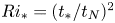 $Ri_* = ( {t}_*/ {t}_N)^2$, and then derived a relationship for destratification rate
 ${\mathcal {D}}_N$ of the form
 \[ {\mathcal{D}}_N = C_1Ri_{\tau}^{-1} + C_2Ri_*^{-1}, \]
where  $C_1 = 2.1$,
 $C_2 = 1.2$. This relationship assumes that the mixing processes due to surface cooling and bed shear can be modelled as being linearly independent. The model is valid for
 $Ri_{\tau } > 15$. Here, the destratification rate,
 ${\mathcal {D}}_N$, is non-dimensionalised in terms of the stratification time scale and the difference between the maximum horizontally averaged temperature in the domain and the horizontally averaged temperature at the channel bottom, that is,
 \[ {\mathcal{D}}_N = -\frac{\textrm{d}\Delta\tilde{\theta}}{\textrm{d} \tilde{t}}\frac{\tilde{t}_N}{\Delta\tilde{\theta}}, \]
where
 \[ \tilde{t}_N(\tilde{t}) = \left(\frac{\tilde{\beta} \tilde{g} \Delta\tilde{\theta}}{\tilde{h}}\right)^{-1/2} \quad \text{and} \quad \Delta\tilde{\theta}(\tilde{t}) = \overline{\tilde{\theta}}_{m} - \overline{\tilde{\theta}}_{b}. \]
We then showed that this relationship can be integrated to give a formula for the time required for the flow to destratify from an initial temperature difference  ${\Delta \tilde {\theta }}_i$ to a final temperature difference
 ${\Delta \tilde {\theta }}_f$. This formula is
 \[ \tilde{t}_d = \frac{2 \left(\tilde{\beta} \tilde{g}\right)^{1/2} \tilde{h}^{3/2} \left({\Delta\tilde{\theta}}_i^{1/2} - {\Delta\tilde{\theta}}_f^{1/2}\right)}{C_1 [\tilde{u}_{\tau}^2]_{av} + C_2 [\tilde{w}_*^2]_{av}}, \]
where  $[\tilde {u}_{\tau }^2]_{av}$ and
 $[\tilde {w}_*^2]_{av}$ are the squared friction and convection velocities averaged over the duration of the destratification process.
Comparison of these relations with data from our simulations shows that they accurately predict the destratification rate and destratification time recorded in the simulations across a wide range of  $Ri_{\tau }$ and
 $Ri_*$. Further investigations are required to determine the dependence of these scaling relations on Reynolds and Prandtl number.
Acknowledgments
The authors gratefully acknowledge the support of the Australian Research Council (ARC). The research in this paper was supported by ARC Discovery Project DP150100912. The authors also acknowledge the National Computational Infrastructure (NCI) which is supported by the Australian Government and the Sydney Informatics Hub and high performance computing cluster Artemis at the University of Sydney for providing high performance computing resources and services that have contributed to the research results reported within this paper. Finally, we would like to thank the reviewers, whose useful suggestions have strengthened this paper.
Declaration of interests
The authors report no conflict of interest.
Supplementary movies
Supplementary movies are available at https://doi.org/10.1017/jfm.2020.447.