2. Problem formulation

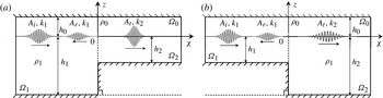
A sketch of the considered problem is presented in figure 1 for two possible configurations, with an incident wave coming from the deeper region (a) or from the shallower region (b). The sharp density interface (the pycnocline) is located at the depth $h_{0}$ beneath the water surface. To filter surface waves we apply the ‘rigid lid approximation’ at the free surface (Brekhovskikh & Goncharov Reference Brekhovskikh and Goncharov1994). All other notations are shown in the figure.

Figure 1.

Sketch of the computational domain: (a) $h_{2}/h_{1}<1$ , a wavetrain propagates from the deeper region to the shallower one; (b) $h_{2}/h_{1}>1$ , a wavetrain propagates from the shallower region to the deeper one.

When a linear quasi-monochromatic wavetrain of amplitude $A_{i}$ and wavenumber $k_{1}$ transforms at the bottom obstacle, two other travelling waves appear. One of them propagates in the same direction as the incident wave, but with the amplitude $A_{t}$ and wavenumber $k_{2}$ in the region with the lower-layer thickness $h_{2}$ . Another wave train propagates in the opposite direction with the amplitude $A_{r}$ and wavenumber $|k_{r}|=|k_{i}|$ in the same region as the incident wave with the lower-layer thickness $h_{1}$ . We considered both the cases when the transformation occurs with the incident wave travelling from the deeper to the shallower region, $h_{2}/h_{1}<1$ , as shown in figure 1(a), and from the shallower to the deeper region, $h_{2}/h_{1}>1$ , as shown in figure 1(b).

We introduce further the following notations for dimensionless parameters which will be used in this paper: $T=A_{t}/A_{i}$ is the transmission coefficient, $R=A_{r}/A_{i}$ is the reflection coefficient, $a={\it\rho}_{0}/{\it\rho}_{1}$ is the density ratio of the upper to the lower layer, ${\it\kappa}=k_{1}h_{1}$ is the normalized wavenumber of the incident wave and $q=k_{2}h_{1}$ is the normalized wavenumber of the transmitted wave.

Assuming that the fluid is perfect and its motion is non-vortical, we can introduce the velocity potentials in each domain: $\boldsymbol{v}_{0}=\boldsymbol{{\rm\nabla}}{\it\varphi}_{0}$ in the upper layer (domain ${\it\Omega}_{0}$ ), $\boldsymbol{v}_{1}=\boldsymbol{{\rm\nabla}}{\it\varphi}_{1}$ in the lower layer in front of the bottom step (domain ${\it\Omega}_{1}$ ) and $\boldsymbol{v}_{2}=\boldsymbol{{\rm\nabla}}{\it\varphi}_{2}$ in the lower layer behind the bottom step (domain ${\it\Omega}_{2}$ ). Then, in each domain the potentials obey the Laplacian equations, ${\rm\Delta}{\it\varphi}_{i}=0$ , where $i=0,1,2$ .

From the impermeability conditions on the rigid surfaces, i.e. on the bottom, the upper surface under the ‘rigid lid approximation’ and the vertical face of the bottom step, it follows that the velocity component normal to the surface should be equal to zero, $\partial {\it\varphi}_{i}/\partial n=0$ .

At the interface between the layers the boundary conditions in the linear approximation are (Lamb Reference Lamb1932; Brekhovskikh & Goncharov Reference Brekhovskikh and Goncharov1994)

where $g$ is the acceleration due to gravity and the index $j=1,2$ pertains to the domains ${\it\Omega}_{1,2}$ shown in figure 1.

The particular solution of the Laplacian equation with the indicated boundary conditions in each domain ${\it\Omega}_{1}$ and ${\it\Omega}_{2}$ far from the edge of the bottom step ( $|x|\rightarrow \infty$ ) can be readily found in the form of a travelling wave:

where the wave frequency ${\it\omega}$ is linked with the wavenumber $k_{j}$ through the dispersion relation (Brekhovskikh & Goncharov Reference Brekhovskikh and Goncharov1994):

As has been conjectured by Lamb (Reference Lamb1932) and further justified rigorously by Bartholomeusz (Reference Bartholomeusz1958) and Miles (Reference Miles1967), for infinitely long surface waves the transformation coefficients can be readily derived from the conditions of mass conservation and pressure continuity at the vertical boundary $x=0$ between the deeper and shallower layers. The same approach is applicable to internal waves and has been used already in the paper by Grimshaw et al. (Reference Grimshaw, Pelinovsky and Talipova2008) to derive the transformation coefficients in two-layer fluid with small density difference between the layers (i.e. in the Boussinesq approximation). In general, the transformation coefficients for very long waves can be presented in terms of wave velocities:

where $c_{1}$ is the wave velocity in front of the bottom step and $c_{2}$ is that behind it. The wave velocities can be found from the dispersion relation (2.3) in the long-wave limit when $k_{j}\rightarrow 0$ (note that in such limit there is no difference between the group and phase velocities):

Substituting these expressions into (2.4) we obtain

From the condition of frequency conservation in a stationary medium we obtain in the same long-wave limit the relationship between the wavenumbers of incident and transmitted waves (the absolute values of wavenumbers of reflected and incident waves obviously are equal): $k_{2}/k_{1}=1/Q_{l}$ .

In the Boussinesq approximation when ${\it\rho}_{0}\approx {\it\rho}_{1}~(a\approx 1)$ (2.6) reduce to the equation derived in Grimshaw et al. (Reference Grimshaw, Pelinovsky and Talipova2008) with

In another limiting case when ${\it\rho}_{0}\rightarrow 0~(a\rightarrow 0)$ (2.6) reduce to the Lamb formulae for long surface waves with $Q_{l}=\sqrt{h_{2}/h_{1}}$ .

The dependences of the transformation coefficients and the wavenumbers of the transmitted wave on hydrological parameters will be presented and analysed in § 3.

3. Derivation of approximative formulae

In the general case of arbitrary wavelength the derivation of transformation coefficients requires consideration of not only the travelling waves, but also the evanescent modes clasped to the edge of the bottom step (Bartholomeusz Reference Bartholomeusz1958; Kurkin et al. Reference Kurkin, Semin and Stepanyants2015). This problem has not been solved yet for internal waves. In the meantime, even in the case of surface wave transformation, despite well-developed rigorous theory, the transformation coefficients cannot be presented in the analytical form. Therefore, for practical applications it is more convenient to use approximate formulae which may provide sufficient accuracy. Such formulae providing 5 % accuracy for the transmission coefficient were suggested in the papers by Miles (Reference Miles1967), Giniyatullin et al. (Reference Giniyatullin, Kurkin, Semin and Stepanyants2014) and Kurkin et al. (Reference Kurkin, Semin and Stepanyants2015). Here, we suggest approximative formulae similar to those that have been used to approximate the data of direct numerical modelling of surface wave transformation (Giniyatullin et al. Reference Giniyatullin, Kurkin, Semin and Stepanyants2014; Kurkin et al. Reference Kurkin, Semin and Stepanyants2015).

The key points for the construction of approximative formulae are Lamb’s formulae in the form of (2.4). As has been mentioned above, these formulae are correct in the limiting case of infinitely long waves, when there is no difference between the group and phase velocities. For waves of arbitrary wavelength the dispersion effect becomes important, and the group and phase velocities are not equal. We assume, however, that Lamb’s formulae remain in the same form, but instead of long-wave velocities we suggest the use of either group velocities for the transmission coefficient or phase velocities for the reflection coefficient. This choice has been made on the basis of a trial and error method and validated by comparison with the numerical data (see below).

The phase and group velocities ( $V_{p}\equiv {\it\omega}/k_{j}$ and $V_{g}\equiv \text{d}{\it\omega}/\text{d}k_{j}$ respectively) can be found from the dispersion relation (2.3):

By substituting the group velocities (3.2) into the Lamb formula for the transmission coefficient (2.4) instead of $c_{1,2}$ and phase velocities (3.1) for the reflection coefficient, we obtain

where

These formulae should be used together with the frequency conservation law, which leads to the transcendental equation for the calculation of the wavenumber of the transmitted wave:

Equation (3.5) should be solved first by means of any numerical software. Then, the calculated wavenumber $k_{2}$ can be substituted into (3.3) and (3.4) for the transformation coefficients.

The formulae (3.4) and (3.5) naturally reduce to the corresponding expressions for surface gravity waves published in Giniyatullin et al. (Reference Giniyatullin, Kurkin, Semin and Stepanyants2014) and Kurkin et al. (Reference Kurkin, Semin and Stepanyants2015) when the density of the upper layer vanishes, $a\rightarrow 0$ . In another limiting case when the layer densities are almost equal ( $a\approx 1$ ) we obtain the transformation coefficients in the Boussinesq approximation. The detailed analysis and verification of the transformation coefficient suggested here will be presented in § 5.

In conclusion of this section we notice that the energy flux is conserved in the process of wave propagation and transformation in conservative media when the energy dissipation is neglected. In the recent paper by Kurkin et al. (Reference Kurkin, Semin and Stepanyants2015) the law of energy flux conservation has been derived for surface waves experiencing a transformation on the bottom step. Obviously, the same law can be derived for internal waves too when the dissipation is negligible. Using the solutions of the linearized equations for a two-layer fluid (2.2), one can derive the period averaged energy density of an internal wave (see, e.g., Stepanyants Reference Stepanyants1985): $E_{j}={\it\rho}_{1}g(1-a)A_{j}^{2}/2$ . The energy flux is the product of the energy density and the group velocity, ${\it\Pi}=EV_{g}$ . After that the law of energy flux conservation can be presented in the form $V_{g1}A_{i}^{2}=V_{g1}A_{r}^{2}+V_{g2}A_{t}^{2}$ , where the left-hand side is the energy flux in the incident wave and the right-hand side is the sum of energy fluxes in the reflected and transmitted waves.

From this equation there follows an important relationship between the transformation coefficients:

If the energy flux is conserved, then from this formula we obtain the equality

Therefore, the quantity $F$ can be used as an indicator of how accurate the derived formulae for the transformation coefficients are. In particular, on substituting the coefficients (2.6) for long waves into (3.7), one can readily see that $F=1$ and does not depend on any parameter. In § 5 we present a comparison of our approximative formulae (3.3)–(3.5) and numerical data with the law of energy flux conservation in the form of (3.7).

4. Numerical model set-up

For the modelling of the wave transformation we utilized the fully nonlinear numerical code MITgcm, which is based on solution of the Navier–Stokes equation for internal waves in the Boussinesq approximation. We assumed that the fluid is perfect and incompressible. A detailed description of the code can be found in Marshal et al. (Reference Marshal, Hill, Perelman and Adcroft1997) and Adcroft et al. (Reference Adcroft, Campin, Dutkiewicz, Evangelinos, Ferreira, Forget, Fox-Kemper, Heimbach, Hill, Hill, Jahn, Losch, Marshal, Maze, Menemenlis and Molod2008). A sketch of the computational domain is shown in figure 1. Impermeable and free-slip boundary conditions were imposed at all solid boundaries, including the left and right walls.

The fluid density was chosen in consistency with the Boussinesq approximation, ${\it\rho}_{0}=0.9961{\it\rho}_{1}$ . The initial wavetrain was imposed at the interface between the domains ${\it\Omega}_{0}$ and ${\it\Omega}_{1}$ such that it travelled to the right (see figure 1). The initial wave perturbation was initialized in consistency with linear theory by the functions ${\it\eta}$ and ${\it\varphi}_{0,1}$ as per (2.2), but with the amplitude modulated by the Gaussian envelope, $A(x)={\it\eta}\,\exp [-(x-x_{c})^{2}/D^{2}]$ , where $x_{c}$ is the initial position of the wavetrain in the domain ${\it\Omega}_{1}$ and $D$ is its characteristic width. In our calculations this parameter was chosen such that it was always four times greater than the length of the carrier wave, $D=4{\it\lambda}$ , where ${\it\lambda}=2{\rm\pi}/k_{1}$ . This suggests that the initial wavetrain was quasi-monochromatic, satisfying with a good accuracy the Laplace equation and boundary conditions (see (2.1) and the text above it). The size of the computational domain on the left of the edge of the bottom step was six times greater than $D$ , and on the right it was nine times greater than $D$ .

The horizontal and vertical resolutions were different. The number of grid points in the horizontal direction was chosen such that it was always 20 points per wavelength of the transmitted and reflected waves. In the vertical direction the total number of grid points was 320, and 120 of them were allocated for the fine resolution of the pycnocline. The number of grid points limited the accuracy of the numerical determination of transformation coefficients; their values were determined with an accuracy of 3 %.

When the initial wavetrain commences its motion towards the bottom step, it emits a very-small-amplitude wavetrain propagating in the opposite direction. This is a consequence of the fact that the initial wavetrain is not an exact, but only an approximate, solution to the basic set of equations. It was confirmed that the greater the aspect ratio $D/{\it\lambda}$ was, the smaller the amplitude of the oppositely moving residual wavetrain was. When the basic and residual wavetrains were clearly separated, the amplitude of the wavetrain $A_{i}$ moving towards the bottom step was measured and used then for the amplitude normalization of the transmitted and reflected waves: $T=A_{t}/A_{i}$ and $R=A_{r}/A_{i}$ . After completion of the transformation, the spatial Fourier analysis was performed over sufficiently long horizontal domains containing the transmitted and reflected wavetrains entirely. Then the maximal amplitude $A_{t,r}$ of the wave spectrum was determined and used for calculation of the transformation coefficients $T$ and $R$ .

5. Results and discussion

It is convenient to analyse both the theoretical and the numerical results in the dimensionless form. Using the dimensionless variables introduced in § 2 the approximative formulae derived in § 3 can be presented as follows:

and

whereas the expressions for $D({\it\alpha},{\it\beta},{\it\gamma},{\it\zeta})$ and $E({\it\alpha})$ are determined after (3.4).

We performed 90 numerical runs with different initial wavetrain parameters and pycnocline positions. Below we present the results of calculations for the following dimensionless wavenumbers of the incident wave: ${\it\kappa}=\{0.1,\;1.0,\;10.0\}$ . These wavenumbers illustrate conditionally the transformation of long, moderate and short waves. The relative pycnocline position was chosen as $h_{0}/h_{1}=\{0.1,\;1.0,\;10.0\}$ , which corresponds to the situations when the interface between layers is close to the surface, located in the middle of the first domain or close to the bottom respectively. Then the depths of the lower layer behind the edge of the bottom step varied discretely such that the ratio $h_{2}/h_{1}$ took ten values in the range $h_{2}/h_{1}=\{0.01;\;100\}$ . This range covered the cases when the wavetrain travelled from the deeper layer to the shallower one (five points when $h_{2}/h_{1}<1$ ) and vice versa (the other five points when $h_{2}/h_{1}>1$ ). We determined the wavenumber of the transmitted wave from numerical data and have found that it agrees perfectly with (5.1). 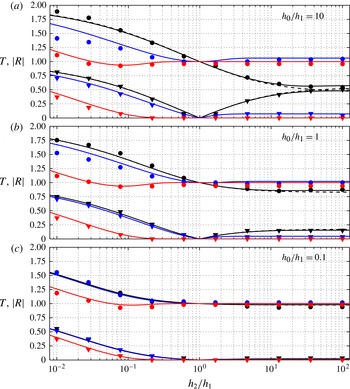Then we determined also the coefficients of transmission $T$ and reflection $R$ ; they are depicted in figure 2.

Figure 2.

Dependences of the transmission coefficient $T$ (circles) and the reflection coefficient $|R|$ (triangles) for the different pycnocline positions: (a) $h_{0}/h_{1}=10$ ;(b) $h_{0}/h_{1}=1$ ; (c) $h_{0}/h_{1}=0.1$ . The solid lines were generated on the basis of the approximate analytical formulae (5.2). The black solid lines pertain to ${\it\kappa}=0.1$ , the blue lines to ${\it\kappa}=1$ and the red lines to ${\it\kappa}=10$ . The black dashed lines in panels (a) and (b) pertain to the limiting case of an infinitely long wave as per (2.6).

In this paper we restrict our analysis to the consideration of wave transformation at small density difference because (i) the numerical code MITgcm is applicable only to a stratified fluid in the Boussinesq approximation and (ii) the influence of density difference becomes noticeable only when ${\it\rho}_{0}/{\it\rho}_{1}<0.1$ . In the meantime, in the limiting case when ${\it\rho}_{0}/{\it\rho}_{1}\rightarrow 0$ the considered problem reduces to the surface wave transformation; this case has already been studied in detail (see the introduction and references therein).

As the first step we have determined the dependence of the transmitted wavenumber on the incident wavenumber as a function of the depth ratio $h_{2}/h_{1}$ for different pycnocline positions. As was expected, the wavelength of the transmitted wave decreases for waves travelling from the deeper to the shallower region and increases in the opposite case. The strongest transformation of wavenumbers occurs in the case of long waves; the effect becomes less pronounced when the wavelength decreases. The wavenumber of the transmitted wave in the long-wave limit ( ${\it\kappa}\rightarrow 0$ and $q\rightarrow 0$ ) can be determined from the formula that follows from (5.1):

In another limiting case of short-wave transformation ( ${\it\kappa}\rightarrow \infty$ and $q\rightarrow \infty$ ) the transmitted wave has the same wavenumber as the incident wave, $q={\it\kappa}$ .

The transmission and reflection coefficients are depicted in figure 2(a) for a pycnocline position such that $h_{0}/h_{1}=10$ . As one can see, the transmission coefficient is a non-monotonic function of the depth ratio $h_{2}/h_{1}$ , in general. Asymptotically, the transformation coefficients approach the limiting values $T\rightarrow 2$ and $|R|\rightarrow 1$ when $h_{2}/h_{1}\rightarrow 0$ . The limiting case $h_{2}/h_{1}=0$ corresponds to the full reflection of a wavetrain from the vertical barrier; in this case instead of transmission we have just wave splash with double amplitude and zero wavelength.

The case of $h_{2}/h_{1}=1$ is trivial – there is no bottom obstacle at all, and a wavetrain does not experience any transformation; it just propagates in a fluid of a uniform depth.

In the case of $h_{2}/h_{1}>1$ the wavetrain travels from the shallower to the deeper water. The characteristic feature of this case is that the transformation coefficients of long waves with ${\it\kappa}\leqslant 0.1$ asymptotically approach values that are close to 0.5 when $h_{2}/h_{1}\rightarrow \infty$ (see figure 2 a). This is in contrast to the transformation coefficients of long surface waves, where the transmission coefficient goes to zero monotonically and the reflection coefficient goes to unity in the same limit (Giniyatullin et al. Reference Giniyatullin, Kurkin, Semin and Stepanyants2014; Kurkin et al. Reference Kurkin, Semin and Stepanyants2015).

The transformation process becomes weaker when the wavelength of the incident wave decreases. As a consequence of this the reflection coefficient vanishes when $h_{2}/h_{1}>1$ and ${\it\kappa}$ increases. The transmission coefficient becomes equal to one – a reflectionless transformation occurs in this case. In the intermediate case of ${\it\kappa}\sim 1$ the transmission coefficient of a wavetrain travelling from shallower to deeper water is slightly greater than 1, whereas the reflection coefficient approaches some small, but non-zero value (see the blue lines and the corresponding circles and triangles in figure 2 a).

There is another peculiarity of short-wave transformation. The transmission coefficient turns to unity not only in the trivial case when $h_{2}/h_{1}=1$ , but also at another depth ratio when $h_{2}/h_{1}<1$ (note that the reflection coefficient is not equal to zero at such a depth ratio). This is clearly seen in figure 2 when ${\it\kappa}=10$ . In such a case the amplitude of the transmitted wave remains the same as the amplitude of the incident wave, but the wavelengths of these two waves are not equal. The same effect has been discovered for surface waves (Giniyatullin et al. Reference Giniyatullin, Kurkin, Semin and Stepanyants2014; Kurkin et al. Reference Kurkin, Semin and Stepanyants2015).

Figure 2 illustrates also the influence of the pycnocline position on the transformation process. As one can see from the figure, the transmission coefficient becomes closer to unity and the reflection coefficient gradually vanishes when the pycnocline position approaches the top rigid surface and the depth ratio $h_{0}/h_{1}$ decreases. The effect is more pronounced for long waves with ${\it\kappa}\leqslant 0.1$ (cf. the black solid lines in all the panels). The clearest manifestation of the effect occurs in the case when $h_{2}/h_{1}>1$ .

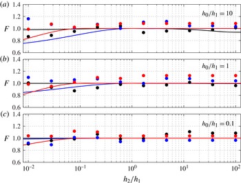
In figure 3 we present the function $F$ as per (3.7), which characterizes the accuracy of energy flux conservation. According to our experience with surface waves (Giniyatullin et al. Reference Giniyatullin, Kurkin, Semin and Stepanyants2014; Kurkin et al. Reference Kurkin, Semin and Stepanyants2015), this function is very sensitive to errors in the determination of the transformation coefficients. Therefore, even small errors in the numerical determination of the transmission and reflection coefficients led to the dots deviating from unity. This explains the scattering of numerical data around the horizontal line $F=1$ . The function $F$ calculated on the basis of the approximative formulae for the transformation coefficients deviates from unity too. The deviation of $F$ from unity is most noticeable for relatively short waves with ${\it\kappa}>0.1$ when $h_{2}/h_{1}\leqslant 0.1$ . In particular, when the pycnocline is close to the bottom ( $h_{0}/h_{1}=10$ ) and ${\it\kappa}=1$ , the deviation of $F$ from unity reaches 22 % at $h_{2}/h_{1}\leqslant 0.01$ (see the blue line in figure 3 a). In all other cases the deviation is smaller.

Figure 3.

The function $F$ as per (3.7), which characterizes the accuracy of energy flux conservation. The panels correspond to different pycnocline positions $h_{0}/h_{1}$ (the same as in figure 2). The solid lines were generated on the basis of the approximative formulae (5.2) and the dots represent the data of direct numerical calculations. The black line pertains to ${\it\kappa}=0.1$ , the blue line to ${\it\kappa}=1$ and the red line to ${\it\kappa}=10$ .

In general, one can conclude that there is a very good agreement between the solution of the transcendental equation (5.1) for the wavenumber of the transmitted wave and the wavenumber values determined from the direct numerical modelling. Moreover, we have obtained a quite satisfactory agreement between the approximative formulae for the transformation coefficients and the results of direct numerical calculations. The discrepancies between the theoretical prediction and the numerical data can be explained by the limited accuracy of the determination of the transformation coefficients from the numerical calculations and the approximate character of the derived theoretical formulae.