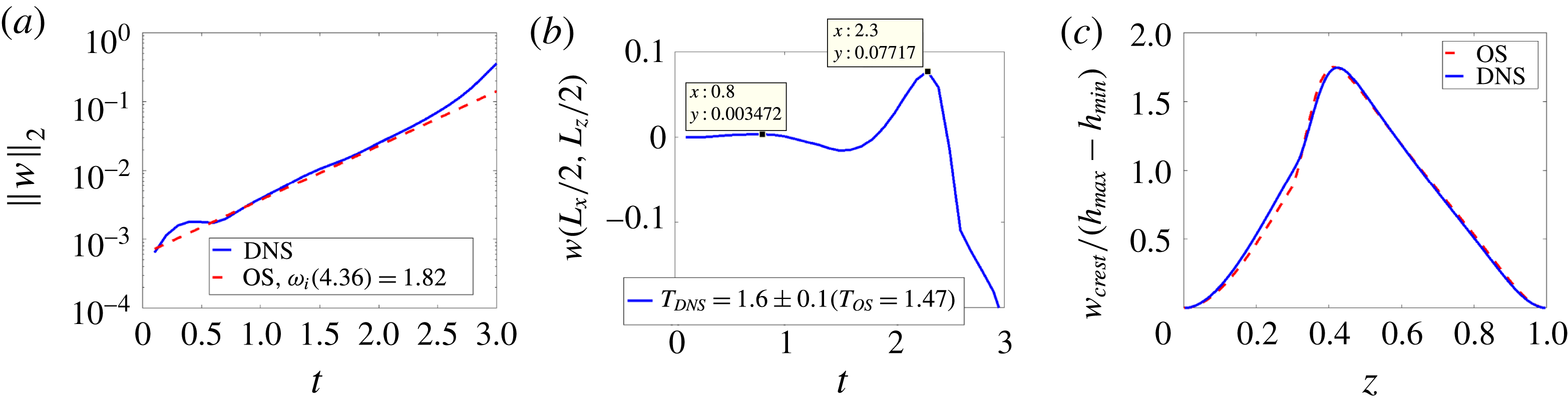
1 Introduction
We study three-dimensional waves in gas–liquid two-layer channel flows driven by a pressure gradient, under stable stratification. In the classical problem of Kelvin–Helmholtz instability, vorticity is confined to a layer about the interface that is assumed to be vanishingly thin on the scale of the wave amplitude (e.g. Batchelor Reference Batchelor1967). In the present study, we assume the flow to be generated not impulsively, but gradually, with vorticity present throughout the unidirectional base flow that is perturbed initially. A motivation of the study is the transition from stable stratified flow, and the subsequent flow behaviour, commonly observed in engineering applications of gas–liquid transport through pipelines (e.g. Hewitt Reference Hewitt and Hetsroni1982). The objective here is to understand the flow behaviour beyond this stable regime. The present study is therefore distinct from other strands in the literature that focus on two-layer flows with very strong spatial inhomogeneity, such as in wave growth downstream from a splitter plate between two fluids, often studied as a model of gas-assisted jet flows (e.g. Fuster et al. Reference Fuster, Matas, Marty, Popinet, Hoepffner, Cartellier and Zaleski2013).
Linear stability analysis of the unidirectional viscous base flow generally indicates that the most amplified disturbance in such systems is two-dimensional in character. Yet beyond a linear regime, a myriad of three-dimensional interfacial phenomena is observed, such as fully three-dimensional nonlinear waves, ligaments and droplet entrainment (Hewitt Reference Hewitt and Hetsroni1982). Therefore, the aim of this work is to understand the instabilities that promote such phenomena in gas–liquid flows, having studied the liquid–liquid (density-matched) systems previously (Ó Náraigh et al. Reference Ó Náraigh, Valluri, Scott, Bethune and Spelt2014). Although Squire’s transformation exists for all such flows (Blennerhassett Reference Blennerhassett1980), instability does not necessarily arise beyond a critical Reynolds number, hence Squire’s theorem does not exist for these systems (Yiantsios & Higgins Reference Yiantsios and Higgins1988). Nevertheless, the most amplified waves in modal linear theory are generally two-dimensional (Sahu & Matar Reference Sahu and Matar2011). The two-dimensional linear stability analysis for this system, involving the Orr–Sommerfeld equations for the two phases subject to pertinent conditions at the evolving interface and the walls, is well established (Yiantsios & Higgins Reference Yiantsios and Higgins1988), as is the corresponding three-dimensional analysis (e.g. Sahu & Matar Reference Sahu and Matar2011).
Classification of the linear instability, by an energy-budget analysis wherein the rate of change of total kinetic energy in the flow per unit wavelength is determined from the linear perturbation equations (Boomkamp & Miesen Reference Boomkamp and Miesen1996), has revealed that for laminar base flows in the present configuration at small to moderate values of Froude and Reynolds numbers (specified below in § 2) the two important ways the perturbed flow extracts kinetic energy from the base state are (e.g. Boomkamp & Miesen Reference Boomkamp and Miesen1996): (i) a viscosity-contrast source due to the viscosity mismatch at the interface (the so-called ‘Yih mode’ after Yih (Reference Yih1967)), which for weakly inertial flows arises from the out-of-phase distribution of the perturbation vorticity (Hinch Reference Hinch1984) – this mechanism is recalled in further detail in § 5.3; and (ii) a shear mode similar to a Tollmien–Schlichting mode in the bulk of one the two layers. Also, a mixture of both mechanisms can arise. In all, viscous effects, which enter the base state as well as the perturbation equations, are key in the growth rate of the primary instability. This is found also in two-layer flow of a gas and liquid that are separated upstream by a splitter plate (Fuster et al. Reference Fuster, Matas, Marty, Popinet, Hoepffner, Cartellier and Zaleski2013).
Elementary linear stability starts with the assumption that the base flow is perturbed by a delocalized sinusoidal disturbance. In practice, disturbances can be localized either in the interior of the flow domain or at the inlet, in which case the basic linear theory must be extended to account for absolute and convective instability and also spatial growth of the disturbances (Huerre & Monkewitz Reference Huerre and Monkewitz1990). Our own prior work in this area for Poiseuille-type flow in channels provides flow-pattern maps delineating the regions of parameter space where absolute or convective instability can be observed (Ó Náraigh, Spelt & Shaw Reference Ó Náraigh, Spelt and Shaw2013a ). The work by Otto, Rossi & Boeck (Reference Otto, Rossi and Boeck2013) does the same thing for the splitter-plate flow geometry, which enables a favourable comparison between the theory and experiments (Matas Reference Matas2015).
In the present work, we examine the behaviour of these flows beyond such a linear regime, possibly towards atomization, for which direct numerical simulation (DNS) is an important tool. Several key studies based on a splitter-plate configuration (e.g. Ling et al.
Reference Ling, Fuster, Zaleski and Tryggvason2017) have already identified various mechanisms at work in the generation of three-dimensional nonlinear interfacial structures. In this prior work it is demonstrated that both fingering at the tip of the waves and ‘tearing’ of liquid sheets are a definite route to three-dimensional interfacial configurations and thence to atomization. Although the tearing of the sheets in these simulations is due to a numerical effect, the argument there is that such numerical tearing is a model for real physical sheet tearing, which occurs in very thin sheets when the disjoining pressure becomes active. Also, the numerical tearing persists consistently at finer and finer grid resolution, lending further robustness to this modelling approach. The present efforts complement this prior work as we focus on a different flow configuration (two-phase channel flow) motivated by other applications, wherein a strong inhomogeneity is not imposed, to determine the stages of wave growth up to and beyond wave overturning therein. Furthermore, we assess the role of the vorticity field in the three-dimensional wave growth, prior understanding being for the two-dimensional system under weak effects of inertia. Our study also uses the density ratio
 $r=\unicode[STIX]{x1D70C}_{liquid}/\unicode[STIX]{x1D70C}_{gas}$
as a key parameter to be varied, and we take
 $r$
in the range 1–1000. The comparison between results for
 $r=1000$
to those for
 $r=1$
is that between gas–liquid and liquid–liquid systems. The intermediate density ratios allow an assessment of the effect of pressurizing the gas on the flow behaviour, and to see whether the values
 $r=10{-}20$
that are used for computational convenience in the existing numerical simulations of putative gas–liquid flows as in Ling et al. (Reference Ling, Fuster, Zaleski and Tryggvason2017), but also in Scardovelli & Zaleski (Reference Scardovelli and Zaleski1999), Boeck et al. (Reference Boeck, Li, López-Pagés, Yecko and Zaleski2007) and Fuster et al.
Reference Fuster, Matas, Marty, Popinet, Hoepffner, Cartellier and Zaleski2013, can be adopted in the present system.
The starting point for the present study is the mathematical model of two-phase stratified channel flow as described below in §§ 2 and 3; the model is based on the fully nonlinear two-phase Navier–Stokes equations. As such, the methodology is twofold: we first of all characterize the linear stability of the system using Orr–Sommerfeld–Squire theory (§ 4), before characterizing the system in the nonlinear regime, using DNS. The strategy of the DNS is to focus on special initial conditions appropriate for simulations in a periodic channel, and to conduct a comprehensive parametric study in two dimensions, outlining (with flow-pattern maps) the different flow behaviours as a function of the problem parameters (§ 5). As the corresponding three-dimensional simulations are computationally more expensive, the insight obtained from the two-dimensional simulations is used to single out special cases for further investigation via three-dimensional DNS (§ 6). The results of the simulations (in all dimensions) are compared and contrasted with the linear theory via Fourier analysis. In § 6 we also view the instability (both linear and nonlinear) from an equivalent point of view, whereby the source of the instability (in both two and three dimensions) can be traced back to the vorticity field.
2 Problem statement and setup of parametric study
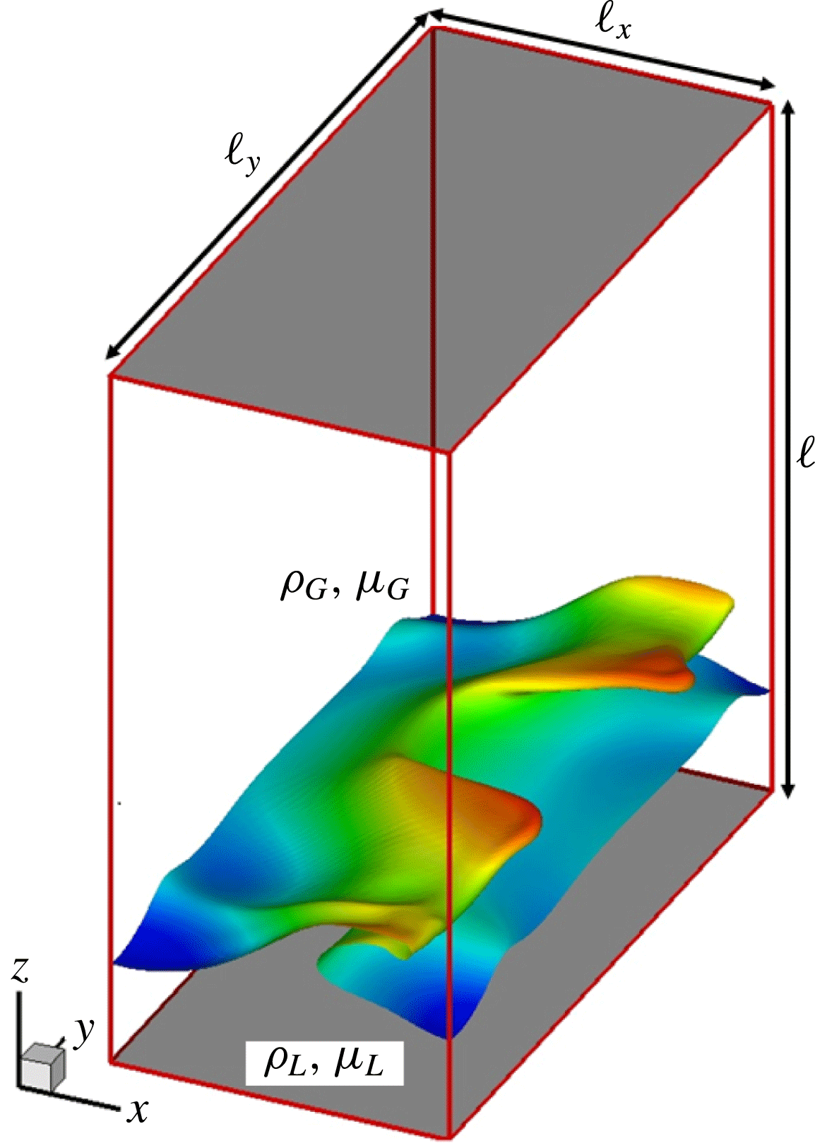
We study here the flow sketched in figure 1. Dimensionless Cartesian coordinates
 $(x,y,z)$
are used over the range
 $[0,\ell _{x}]\times [0,\ell _{y}]\times [0,1]$
, where the channel height
 $\ell$
is used as the characteristic length. We assign labels
 $j=L,G$
to identify properties of the two fluids, with
 $j=L$
for the liquid (bottom) layer and
 $j=G$
for the top (gas) layer. Bounding walls with the implied no-slip boundary conditions are introduced at
 $z=0$
and
 $z=1$
. Periodic boundary conditions are imposed in the spanwise (
 $y$
) direction; periodic boundary conditions modulo a constant pressure drop
 $\text{d}p_{0}/\text{d}x<0$
are imposed in the streamwise (
 $x$
) direction, such that
 $p(x=\ell _{x},y,z)=p(x=0,y,z)+\ell _{x}(\text{d}p_{0}/\text{d}x)$
. The system admits an undisturbed or base-state configuration characterized by a Poiseuille flow where the depth of the undisturbed liquid layer is denoted by
 $h_{0}$
. The system is perturbed away from the base state through the addition of small-amplitude perturbations in the initial conditions. The perturbations either die out (linear stability), or are amplified to produce sustained interfacial waves (linear instability), culminating in the kind of nonlinear structures observed in figure 1. The theory for this is introduced below in § 3. To produce an unstable base-state configuration, a possible approach may be to start with a stable base-state configuration, and to gradually modify a system parameter such that a set of linearly unstable system parameters is reached. For instance, the flow rate could gradually be increased by introduction of a gradual constriction in the channel cross-section (for instance, between the two sides).
Definition sketch showing the three-dimensional problem geometry and the onset of interfacial waves. The domain is periodic in the
 $x$
and
 $y$
directions. A pressure drop drives the flow along the
 $x$
direction. No-slip conditions are applied at
 $z=0$
and
 $z=1$
. The flow is initialized with a two-phase Poiseuille profile and a small-amplitude sinusoidal perturbation around an otherwise flat interface. Waves develop as a result of linear instability and eventually overturn and form the complicated three-dimensional structure shown.

Across interfaces separating the two phases, the following standard jump conditions for the fluid velocity
 $\boldsymbol{u}$
and pressure
 $p$
are satisfied:
 $$\begin{eqnarray}\displaystyle & \displaystyle \unicode[STIX]{x27E6}\widehat{\boldsymbol{n}}\boldsymbol{\cdot }[-p\unicode[STIX]{x1D644}+\unicode[STIX]{x1D707}_{j}(\unicode[STIX]{x1D735}\boldsymbol{u}_{j}+\unicode[STIX]{x1D735}\boldsymbol{u}_{j}^{\text{T}})]\unicode[STIX]{x27E7}\boldsymbol{\cdot }\widehat{\boldsymbol{t}}^{\,(r)}=0,\quad \unicode[STIX]{x27E6}\widehat{\boldsymbol{n}}\boldsymbol{\cdot }[-p\unicode[STIX]{x1D644}+\unicode[STIX]{x1D707}_{j}(\unicode[STIX]{x1D735}\boldsymbol{u}_{j}+\unicode[STIX]{x1D735}\boldsymbol{u}_{j}^{\text{T}})]\boldsymbol{\cdot }\widehat{\boldsymbol{n}}\unicode[STIX]{x27E7}=\unicode[STIX]{x1D6FE}\unicode[STIX]{x1D705}, & \displaystyle \nonumber\\ \displaystyle & & \displaystyle\end{eqnarray}$$
where
 $\widehat{\boldsymbol{n}}$
is a normal vector to the interface (pointing from
 $j=L$
to
 $j=G$
), and
 $\widehat{\boldsymbol{t}}^{\,(1)}$
and
 $\widehat{\boldsymbol{t}}^{\,(2)}$
are the tangent vectors. The brackets
 $\unicode[STIX]{x27E6}\cdot \unicode[STIX]{x27E7}$
denote the jump condition across the interface (
 $(j=G)-(j=L)$
), and
 $\unicode[STIX]{x1D705}$
denotes the interfacial (mean) curvature. Also,
 $\unicode[STIX]{x1D707}_{j}$
denotes the viscosity in the two phases and
 $\unicode[STIX]{x1D6FE}$
is the surface tension.
The constant pressure drop sets a velocity scale
 $V$
in the problem as
 $$\begin{eqnarray}\displaystyle & \displaystyle V=\sqrt{-(\ell /\unicode[STIX]{x1D70C}_{G})(\text{d}p_{0}/\text{d}x)}. & \displaystyle\end{eqnarray}$$
This provides the impetus for identifying non-dimensional flow variables in the problem. Accordingly, we identify the viscosity ratio
 $m=\unicode[STIX]{x1D707}_{L}/\unicode[STIX]{x1D707}_{G}$
and the density ratio
 $r=\unicode[STIX]{x1D70C}_{L}/\unicode[STIX]{x1D70C}_{G}$
. Further important dimensionless groups are a Reynolds number, a gravity parameter and a Weber number. Using the properties of the upper fluid, these are defined as
 $$\begin{eqnarray}\displaystyle & \displaystyle Re={\displaystyle \frac{\unicode[STIX]{x1D70C}_{G}V\ell }{\unicode[STIX]{x1D707}_{G}}},\quad {\mathcal{G}}={\displaystyle \frac{g\ell }{V^{2}}},\quad We={\displaystyle \frac{\unicode[STIX]{x1D70C}_{G}\ell V^{2}}{\unicode[STIX]{x1D6FE}}}={\displaystyle \frac{\ell ^{2}|\text{d}p_{0}/\text{d}x|}{\unicode[STIX]{x1D6FE}}}, & \displaystyle\end{eqnarray}$$
where
 $g$
denotes the dimensional acceleration due to gravity.
The non-dimensionalization as set out in (2.3) is associated with varying the density of the liquid for a given gas layer. The effects of varying instead the density of the gas for a given liquid density can also be determined from the above-mentioned parametric study, in principle, but for one caveat. When scaling on the properties of the liquid, the following further dimensionless groups arise:
 $$\begin{eqnarray}\displaystyle & \displaystyle Re_{L}=\sqrt{r}\,Re/m,\quad {\mathcal{G}}_{L}=r{\mathcal{G}}, & \displaystyle\end{eqnarray}$$
where the meanings of
 $m$
and
 $r$
are unchanged from before. In this context, the dimensionless liquid density and viscosity are unity, and those of the gas are
 $1/r$
and
 $1/m$
, respectively.
The imposed pressure gradient in dimensionless form remains
 $\text{d}p_{0}/\text{d}x$
– hence the factors of
 $\sqrt{r}$
in (2.4) corresponding to a modified velocity scale
 $\sqrt{-(\ell /\unicode[STIX]{x1D70C}_{L})(\text{d}p_{0}/\text{d}x)}$
, but the Weber number is the same regardless of which non-dimensionalization scheme is used, as it is independent of the fluid density and viscosity of either fluid.
The dimensionless groups defined above are all in terms of a characteristic speed defined in terms of the pressure gradient (2.2); the flow rates of gas or liquid cannot be used, as these are not fixed during the DNS. This may seem to render the results difficult to access, but the dimensionless groups used herein can be converted into groups based on superficial gas and liquid velocities for the base-state profiles, which are the volume fluxes divided by the total cross-section of the channel. The ratios of these velocities and
 $V$
defined in (2.2) (for use in redefining the dimensionless groups (2.3) in superficial velocities) are readily obtained from the base-state profiles in § A.1 as
 $$\begin{eqnarray}\displaystyle & \displaystyle {\displaystyle \frac{U_{SG}}{V}}={\displaystyle \frac{1}{6}}Re(1-h_{0})^{3}-{\displaystyle \frac{1}{2}}B(1-h_{0})^{2},\quad {\displaystyle \frac{U_{SL}}{V}}={\displaystyle \frac{Re}{2m}}h_{0}^{3}+{\displaystyle \frac{1}{2}}Ah_{0}^{2}, & \displaystyle\end{eqnarray}$$
where
 $A$
and
 $B$
are given in § A.1. Reynolds numbers based on superficial velocities are then readily obtained as
 $Re_{SG}=(U_{SG}/V)Re$
and the corresponding expression for
 $Re_{SL}$
.
The ranges of values of these parameters studied here are as follows. We restrict our attention to cases wherein
 $1\leqslant r\leqslant 1000$
(thus the gas above the liquid) throughout this study, and take the lower fluid to be the more viscous one, with
 $m=50$
; the dimensionless depth of the undisturbed liquid layer is set to
 $h_{0}=0.2$
. We start parametric studies in subsequent sections by assessing the effects of varying the density of the lower fluid for a given gas by varying the value of
 $r$
therein. At a given value of
 $Re$
, increasing the value of
 $r$
here results in a larger value of the Reynolds number
 $Re_{L}$
and gravity parameter
 ${\mathcal{G}}_{L}$
based on liquid properties, as defined by (2.4), whereas the gas flow is little affected. The Reynolds number based on the properties of the gas will be varied also, over the range
 $100\leqslant Re\leqslant 500$
, with the gravity parameter
 ${\mathcal{G}}=0.1$
.
For air under standard conditions, for the characteristic speed
 $V=(\unicode[STIX]{x1D707}_{G}gRe/(\unicode[STIX]{x1D70C}_{G}{\mathcal{G}}))^{1/3}$
this corresponds to the range
 $0.6{-}1~\text{m}~\text{s}^{-1}$
, and for the channel height
 $\ell ={\mathcal{G}}V^{2}/g$
values between 0.4 and 1 cm. The corresponding superficial gas velocity (obtained from (2.5)) is then between 4 and
 $22~\text{m}~\text{s}^{-1}$
and the Reynolds number
 $Re_{SG}$
is varied between 340 and 8700; at
 $r=1000$
, the Reynolds number based on the superficial liquid velocity is then in the range
 $8\leqslant Re_{SL}\leqslant 212$
. The surface tension follows from the Weber number. We shall start with very weak surface tension by setting
 $We=10$
, which yields for the surface tension
 $\unicode[STIX]{x1D6FE}=\unicode[STIX]{x1D70C}_{G}\ell V^{2}/We$
values in the range
 $10^{-3}{-}10^{-4}~\text{N}~\text{m}^{-1}$
, but then consider realistic values by setting
 $We=1/7$
, which yields the range
 $0.008{-}0.07~\text{N}~\text{m}^{-1}$
. At moderate or low values of
 $r$
, the results would be relevant to systems of compressed gases, for which the values of physical parameters in dimensional form can be determined as outlined above.
As the parametric study outlined above amounts to only one cross-section in parameter space, and may involve values of the liquid density at small
 $r$
that may seem artificial when not considering gases of elevated density, we also assess the effects of varying the density of the gas for a given liquid density. In this context, we use
 $Re_{L}$
and
 ${\mathcal{G}}_{L}$
defined in (2.4) (the definition of Weber number being unaffected), whereas the meanings of
 $m$
and
 $r$
are unchanged from before; the dimensionless liquid density and viscosity are unity, and those of the gas are
 $1/r$
and
 $1/m$
, respectively. Therefore, in this (second) parametric study, effects of inertia and gravity in the gas are reduced when increasing
 $r$
, as is clear when inferring the values of
 $Re$
and
 ${\mathcal{G}}$
from (2.4). We shall present results in this parametric study still in terms of scaling with the gas properties, however (the corresponding values of
 $Re$
and
 ${\mathcal{G}}$
are obtained from (2.4)). We consider the parameter range
 $10\leqslant Re_{L}\leqslant 150$
,
 ${\mathcal{G}}_{L}=1$
, for weak and stronger surface tension,
 $We=10$
or
 $1/7$
. For an example application to air–water systems, near
 $r=10^{3}$
this then gives
 $16\leqslant Re\leqslant 240$
and
 ${\mathcal{G}}=10^{-3}$
, hence
 $V$
(obtained as above) between 1.5 and
 $3.6~\text{m}~\text{s}^{-1}$
and the channel height of the order of 1 mm; the Reynolds-number-based superficial gas velocity is then in the range between 10 and 2000, that for the liquid between 0.2 and 50, and the surface tension between
 $3\times 10^{-3}$
and
 $0.1~\text{N}~\text{m}^{-1}$
. When considering lower values of
 $r$
at
 $Re_{L}$
fixed,
 $Re_{SG}$
is elevated whereas
 $Re_{SL}$
remains fixed.
3 Methodology
Two complementary approaches are used in solving the two-phase Navier–Stokes equations with a density contrast and the jump conditions (2.1); these are described here. These are extensions of the corresponding approaches developed in our previous work (Ó Náraigh et al. Reference Ó Náraigh, Valluri, Scott, Bethune and Spelt2014), to account for a density contrast.
3.1 Modal linear stability analysis
We use linear theory to study the early-time development of three-dimensional disturbances: the stability of the basic Poiseuille flow to small-amplitude disturbances is investigated by solving the linearized equations of motion in the disturbance velocity and pressure fields. Using eigenvalue analysis and the linearized equations of motion for a reduced set of variables (the wall-normal velocity and vorticity), it can be shown that the small-amplitude disturbances grow or decay exponentially, with growth rates and phase speeds determined from a modal Orr–Sommerfeld–Squire (OSS) eigenvalue analysis, given here in generic form for the eigenvalue
 $\unicode[STIX]{x1D706}$
:
 $$\begin{eqnarray}\displaystyle & \displaystyle \unicode[STIX]{x1D706}\left(\begin{array}{@{}cc@{}}\widehat{M}_{OS} & 0\\ \widehat{M}_{C} & \widehat{M}_{S}\end{array}\right)\left(\begin{array}{@{}c@{}}\widetilde{w}_{\unicode[STIX]{x1D6FC}\unicode[STIX]{x1D6FD}}(z,\unicode[STIX]{x1D706})\\ \widetilde{\unicode[STIX]{x1D702}}_{\unicode[STIX]{x1D6FC}\unicode[STIX]{x1D6FD}}(z,\unicode[STIX]{x1D706})\end{array}\right)=\left(\begin{array}{@{}cc@{}}\widehat{L}_{OS} & 0\\ \widehat{L}_{C} & \widehat{L}_{S}\end{array}\right)\left(\begin{array}{@{}c@{}}\widetilde{w}_{\unicode[STIX]{x1D6FC}\unicode[STIX]{x1D6FD}}(z,\unicode[STIX]{x1D706})\\ \widetilde{\unicode[STIX]{x1D702}}_{\unicode[STIX]{x1D6FC}\unicode[STIX]{x1D6FD}}(z,\unicode[STIX]{x1D706})\end{array}\right), & \displaystyle\end{eqnarray}$$
where
 $\widetilde{w}_{\unicode[STIX]{x1D6FC}\unicode[STIX]{x1D6FD}}$
denotes the wall-normal perturbation velocity and
 $\widetilde{\unicode[STIX]{x1D702}}_{\unicode[STIX]{x1D6FC}\unicode[STIX]{x1D6FD}}$
denotes the wall-normal vorticity. The operator
 $\widehat{L}_{OS}$
depends on wavenumbers and the wall-normal derivative,
 $\widehat{L}_{OS}=\widehat{L}_{OS}[\text{i}\unicode[STIX]{x1D6FC},\text{i}\unicode[STIX]{x1D6FD},\unicode[STIX]{x2202}_{z}]$
(similarly for the other operators). Following standard notation,
 $\unicode[STIX]{x1D6FC}$
denotes a wavenumber in the streamwise direction and
 $\unicode[STIX]{x1D6FD}$
denotes a wavenumber in the spanwise direction. Also, the base state implicit in (3.1) is the analytically computed basic Poiseuille profile. For wall-bounded flows, solution of (3.1) for the eigenvalue
 $\unicode[STIX]{x1D706}$
gives a discrete family of eigenvalues for each Fourier mode,
 $\{\unicode[STIX]{x1D706}_{n}(\unicode[STIX]{x1D6FC},\unicode[STIX]{x1D6FD})\}_{n=0}^{\infty }$
. The growth rate is then determined by the eigenvalue with the largest real part,
 $\unicode[STIX]{x1D706}=-\text{i}\unicode[STIX]{x1D714}$
, with
 $\unicode[STIX]{x1D714}_{i}$
being the growth rate. This approach is standard and is not discussed further here. However, for completeness, the details concerning the base state, the linearized equations of motion and the numerical solution method are provided in appendix A.
3.2 Direct numerical simulation
Beyond linear theory, a level set method with a continuous surface tension model (Sussman & Fatemi Reference Sussman and Fatemi1999) is used as a model for the two-phase Navier–Stokes equations with the interfacial conditions (2.1):
 $$\begin{eqnarray}\displaystyle & \displaystyle \unicode[STIX]{x1D70C}(\unicode[STIX]{x1D719})\left({\displaystyle \frac{\unicode[STIX]{x2202}\boldsymbol{u}}{\unicode[STIX]{x2202}t}}+\boldsymbol{u}\boldsymbol{\cdot }\unicode[STIX]{x1D735}\boldsymbol{u}\right)=-\unicode[STIX]{x1D735}p+{\displaystyle \frac{1}{Re}}\unicode[STIX]{x1D735}\boldsymbol{\cdot }[\unicode[STIX]{x1D707}(\unicode[STIX]{x1D735}\boldsymbol{u}+\unicode[STIX]{x1D735}\boldsymbol{u}^{\text{T}})]+{\displaystyle \frac{1}{We}}\unicode[STIX]{x1D6FF}_{\unicode[STIX]{x1D716}}(\unicode[STIX]{x1D719})\unicode[STIX]{x1D705}\widehat{\boldsymbol{n}}-{\mathcal{G}}\unicode[STIX]{x1D70C}(\unicode[STIX]{x1D719})\widehat{\boldsymbol{z}}, & \displaystyle \nonumber\\ \displaystyle & & \displaystyle\end{eqnarray}$$
 $$\begin{eqnarray}\displaystyle & \displaystyle \unicode[STIX]{x1D735}\boldsymbol{\cdot }\boldsymbol{u}=0, & \displaystyle\end{eqnarray}$$
 $$\begin{eqnarray}\displaystyle \widehat{\boldsymbol{n}}={\displaystyle \frac{\unicode[STIX]{x1D735}\unicode[STIX]{x1D719}}{|\unicode[STIX]{x1D735}\unicode[STIX]{x1D719}|}},\quad \unicode[STIX]{x1D705}=-\unicode[STIX]{x1D735}\boldsymbol{\cdot }\widehat{\boldsymbol{n}},\quad {\displaystyle \frac{\unicode[STIX]{x2202}\unicode[STIX]{x1D719}}{\unicode[STIX]{x2202}t}}+\boldsymbol{u}\boldsymbol{\cdot }\unicode[STIX]{x1D735}\unicode[STIX]{x1D719}=0, & & \displaystyle\end{eqnarray}$$
where
 $\widehat{\boldsymbol{z}}$
is the unit vector in the
 $z$
direction. Here also,
 $\unicode[STIX]{x1D719}(\boldsymbol{x},t)$
is the level set function indicating in which phase the point
 $\boldsymbol{x}$
lies (
 $\unicode[STIX]{x1D719}<0$
in the liquid (bottom) layer,
 $\unicode[STIX]{x1D719}>0$
in the top layer). The (possibly multivalued) interface
 $\unicode[STIX]{x1D709}(\boldsymbol{x},t)$
is therefore the zero level set,
 $\unicode[STIX]{x1D719}(\boldsymbol{x},t)=0~\;\Longrightarrow \;~\boldsymbol{x}=(x,y,\unicode[STIX]{x1D709}(x,y,t))$
. Moreover, the level set function determines the unit vector normal to the interface
 $\widehat{\boldsymbol{n}}$
, as well as the density and viscosity, via the relations
 $\unicode[STIX]{x1D70C}=r(1-H_{\unicode[STIX]{x1D716}}(\unicode[STIX]{x1D719}))+H_{\unicode[STIX]{x1D716}}(\unicode[STIX]{x1D719})$
and
 $\unicode[STIX]{x1D707}=m(1-H_{\unicode[STIX]{x1D716}}(\unicode[STIX]{x1D719}))+H_{\unicode[STIX]{x1D716}}(\unicode[STIX]{x1D719})$
, respectively. The function
 $H_{\unicode[STIX]{x1D716}}(\unicode[STIX]{x1D719})$
is a regularized Heaviside function, which is smooth across a width
 $\unicode[STIX]{x1D716}=1.5\unicode[STIX]{x0394}x$
. Finally,
 $\unicode[STIX]{x1D6FF}_{\unicode[STIX]{x1D716}}(s)=\text{d}H_{\unicode[STIX]{x1D716}}(s)/\text{d}s$
is a regularized delta function supported on an interval
 $[-\unicode[STIX]{x1D716},\unicode[STIX]{x1D716}]$
.
Equations (3.2) are solved in a density-contrast implementation of the computational framework TPLS (Ó Náraigh et al.
Reference Ó Náraigh, Valluri, Scott, Bethune and Spelt2013b
, Reference Ó Náraigh, Valluri, Scott, Bethune and Spelt2014). Specifically, the equations are discretized in space using an isotropic MAC grid wherein vector quantities are defined at cell faces and scalar quantities at the respective cell centres. In terms of the temporal discretization, a third-order Adams–Bashforth scheme is used to treat the convective derivative, while the momentum fluxes are treated using the Crank–Nicolson method. Pressure and the associated incompressibility of the flow are treated using a standard projection method (Chorin Reference Chorin1968). This computational methodology concerning the basic hydrodynamics is explained in an expository fashion in Fannon et al. (Reference Fannon, Loiseau, Valluri, Bethune and Ó Náraigh2016). The level set function is advected using a third-order (fifth-order accurate) weighted essentially non-oscillatory (WENO) scheme (Jiang & Shu Reference Jiang and Shu1996), which is subsequently reinitialized using a Hamilton–Jacobi equation. For the simulations at low surface tension (specifically,
 $We=10$
), the reinitialization methods of Sussman & Fatemi (Reference Sussman and Fatemi1999) and Russo & Smereka (Reference Russo and Smereka2000) give identical results; the results presented herein at high values of
 $We$
are based on the first of these methods. Differences arise in simulations at high surface tension (specifically,
 $We=1/7$
); in those cases the second of these methods is more accurate (Solomenko et al.
Reference Solomenko, Spelt, Ó Náraigh and Alix2017), and the results presented herein are based on this second method. Validation tests similar to those in Ó Náraigh et al. (Reference Ó Náraigh, Valluri, Scott, Bethune and Spelt2014) have been performed for density-contrasted flows and the code is shown to agree excellently with linear OSS theory. Further validation of the code particular to ligament formation in density-contrasted flows has been carried out with respect to benchmarks in the literature, where the code again shows excellent agreement with established numerical test cases. Further details of these tests are given in Solomenko et al. (Reference Solomenko, Spelt, Ó Náraigh and Alix2017).
Throughout this work, unless indication is given to the contrary, a uniform grid is used and the number of grid points in the
 $z$
direction is
 $320$
–
 $340$
. The length of the channel corresponds to the most dangerous mode from linear theory and the width is
 $\ell _{y}=1$
. The time steps used vary in a range
 $10^{-5}{-}10^{-6}$
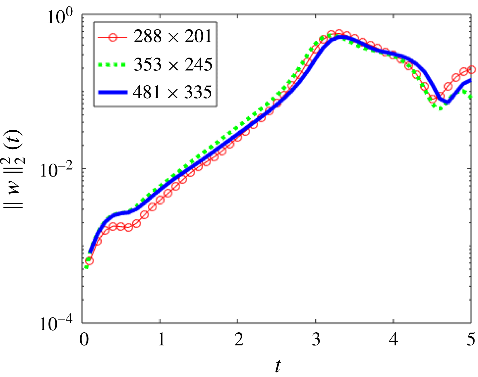
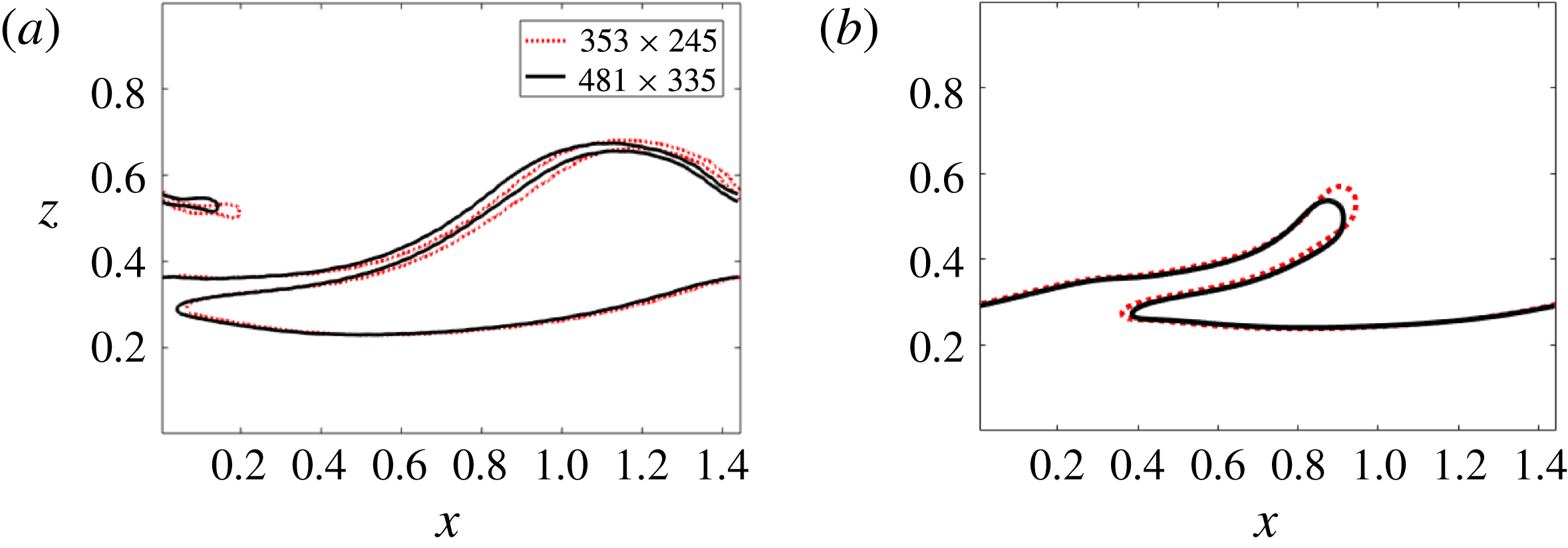
, sufficient to guarantee the stability of the numerical method with respect to the Courant–Friedrichs–Lewy (CFL) condition. These numerical parameters are found to be sufficient to ensure convergence of the numerical method, as described in a sample grid-refinement study in appendix B.
4 Early-stage wave growth – modal linear stability analysis
We compare and contrast the linear stability characteristics for liquid–liquid systems (
 $r=1$
) and gas–liquid systems (
 $r>1$
), since the former is a reference case already considered in detail in Ó Náraigh et al. (Reference Ó Náraigh, Valluri, Scott, Bethune and Spelt2014), in the framework of both linear theory and full-scale DNS. Linear stability analysis is valid during early-stage wave growth when interfacial waves are triggered due to small perturbations in the initial conditions. Unstable waves then grow over time and develop into large-amplitude disturbances, which must be studied by other means, e.g. DNS.
As such, the focus of the present section is on modal (eigenvalue) linear stability analysis. Although this has been analysed previously (e.g. Yiantsios & Higgins Reference Yiantsios and Higgins1988), that prior work is mostly on the neutral stability boundaries for two-dimensional disturbances, and it appears not possible to obtain a comprehensive overview from that for the present purposes, which necessarily involves characterization of instability for a broad range of density contrasts including three-dimensional modes. A concise review is presented based on a comprehensive parametric study for the range of parameter values set out in § 2.
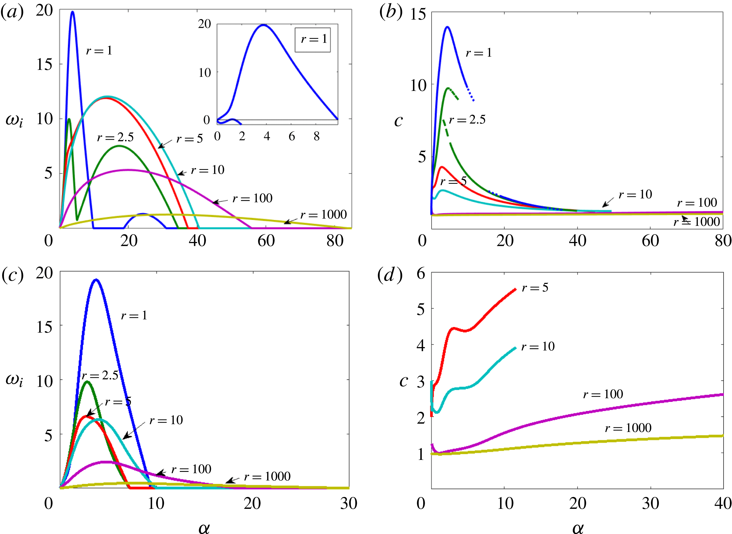
Streamwise-only eigenvalue analyses obtained from solving the Orr–Sommerfeld equation. The scaling is based on the upper-layer properties, for
 $(m,Re,h_{0},{\mathcal{G}})=(50,500,0.2,0.1)$
, and for various values of the density ratio
 $r$
and the Weber number. Panels show (a,c) growth rates and (b,d) wave speeds for (a,b)
 $We=10$
and (c,d)
 $We=1/7$
. The inset in (a) is used to show a third unstable mode for
 $r=1$
, while the broken line in (b) for
 $r=2.5$
is used to indicate the wave speed of the second most dangerous mode.

The neutral modal stability for the two-dimensional two-layer problem has been comprehensively discussed in Yiantsios & Higgins (Reference Yiantsios and Higgins1988) for a broad range of parameter values, albeit only for modest density ratios. For a gas over a liquid layer, considered herein, the upper fluid is not more dense or viscous than the lower fluid, hence within the very broad scope studied in Yiantsios & Higgins (Reference Yiantsios and Higgins1988), we focus on
 $r\geqslant 1$
and
 $m\geqslant 1$
; the liquid layer is not assumed to be very thin. Despite these restrictions, a simple criterion for instability is not available for these systems, as this involves all dimensionless groups. We can merely conclude generally from Yiantsios & Higgins (Reference Yiantsios and Higgins1988) that the flow can be unstable for
 $m>1$
. Based on the same work, and when ignoring effects of gravity and surface tension, we can also conclude that the flow is unstable to long waves at any Reynolds number if
 $m>h_{0}^{2}/(1-h_{0})^{2}$
and, if
 $r\leqslant m^{2}$
, also to short waves. For the ranges of parameter values set out in § 2, the flow is usually unstable, and the neutral curve can be reached usually by descending further to Reynolds numbers lower than considered mostly herein (the neutral curve is shown explicitly in the context of flow-pattern maps in § 5). The main mechanism for instability is often found in prior work to be that of Yih (Reference Yih1967), whereby kinetic energy is gained by a wave from the base flow through the continuity of tangential stress at the interface, whereas an unstable shear (Tollmien–Schlichting type) mode may also arise in the gas beyond a critical Reynolds number (see Boomkamp & Miesen (Reference Boomkamp and Miesen1996) for a review).
For the density-matched case used presently as a reference, a Reynolds number is rather large, so Yih-type and shear modes are both found to be unstable. This is exemplified in figure 2(a), where for
 $r=1$
maxima at
 $\unicode[STIX]{x1D6FC}=3.8$
and
 $\unicode[STIX]{x1D6FC}=24.2$
are observed. These maxima correspond to distinct modal branches of the dispersion relation: an energy budget (Boomkamp & Miesen Reference Boomkamp and Miesen1996) indicates that the less unstable mode is a
 $TAN$
mode of the type of Yih (Reference Yih1967), while the most unstable mode is a shear mode that derives most of its energy from the
 $REY_{G}$
wave Reynolds-stress contribution (these concepts are standard (Boomkamp & Miesen Reference Boomkamp and Miesen1996) but are summarized briefly in § A.3). A third local maximum is observed at
 $\unicode[STIX]{x1D6FC}=1.25$
with a very small growth rate (
 $\unicode[STIX]{x1D714}_{i}=0.11$
, inset of figure 2
a); this is also found to be a gas-side shear mode which emerges at a critical Reynolds number
 $Re\approx 490$
. These modal branches differ further by their wave speed, with the shear mode(s) propagating faster than the Yih mode (see figure 2
b). Surface tension is not expected to have a significant effect on a shear mode; this is confirmed here by comparing results for
 $We=10$
in figure 2(a) with its counterpart for
 $We=1/7$
in figure 2(c), which shows that for (near-) density-matched fluids the maximum growth rate is virtually the same.
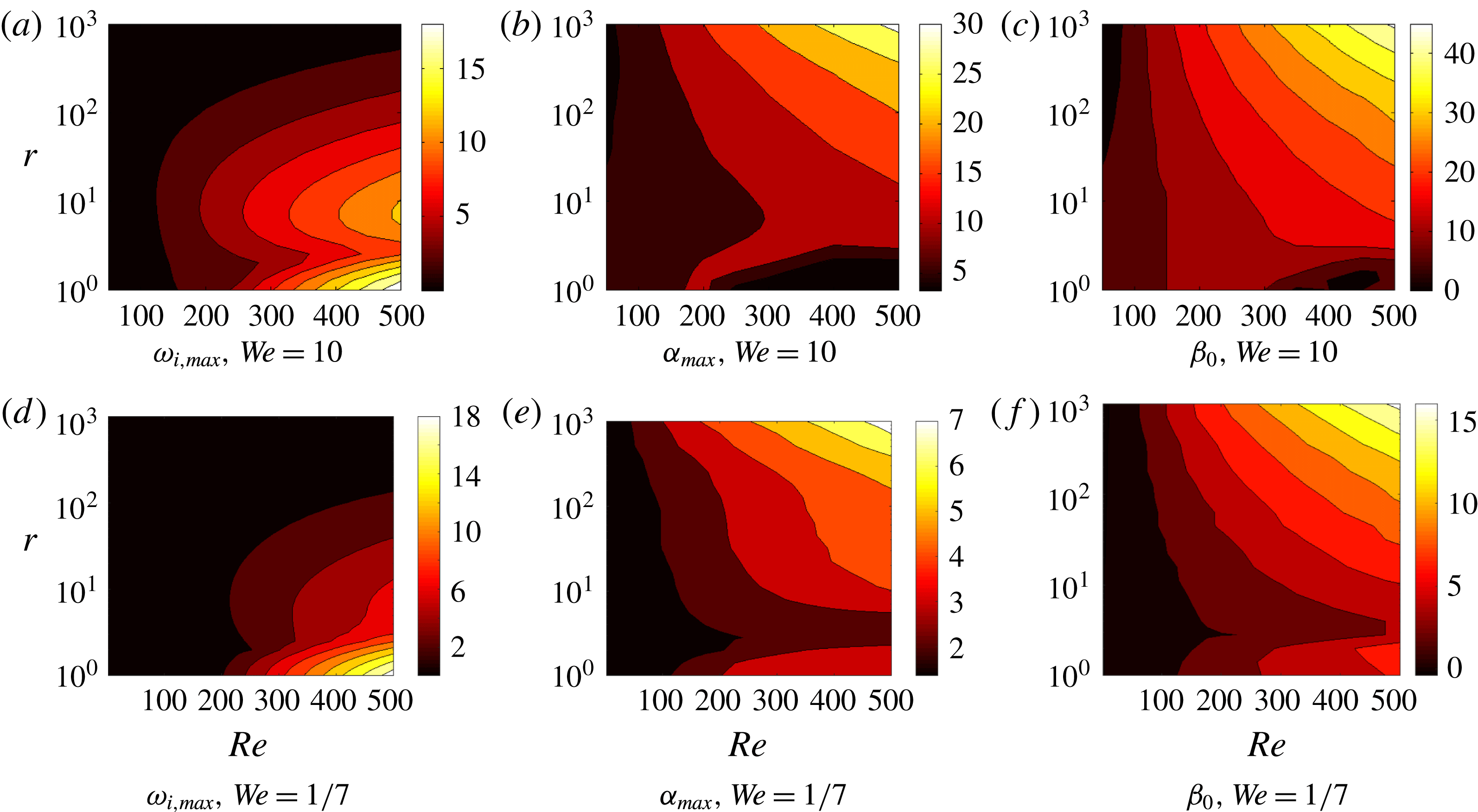
Eigenvalue analysis of the linear system for scaling based on the upper-layer properties. A scan through the
 $Re$
–
 $r$
subspace is shown for the case with
 $(m=50,h_{0}=0.2,{\mathcal{G}}=0.1)$
. (a,d) Maximum (streamwise) growth rate
 $\unicode[STIX]{x1D714}_{i,max}$
; (b,e) the corresponding wavenumber
 $\unicode[STIX]{x1D6FC}_{max}$
; (c,f) the corresponding cutoff spanwise wavenumber
 $\unicode[STIX]{x1D6FD}_{0}$
– i.e. the value of
 $\unicode[STIX]{x1D6FD}$
such that
 $\unicode[STIX]{x1D714}_{i}(\unicode[STIX]{x1D6FC}_{max},\unicode[STIX]{x1D6FD})=0$
.

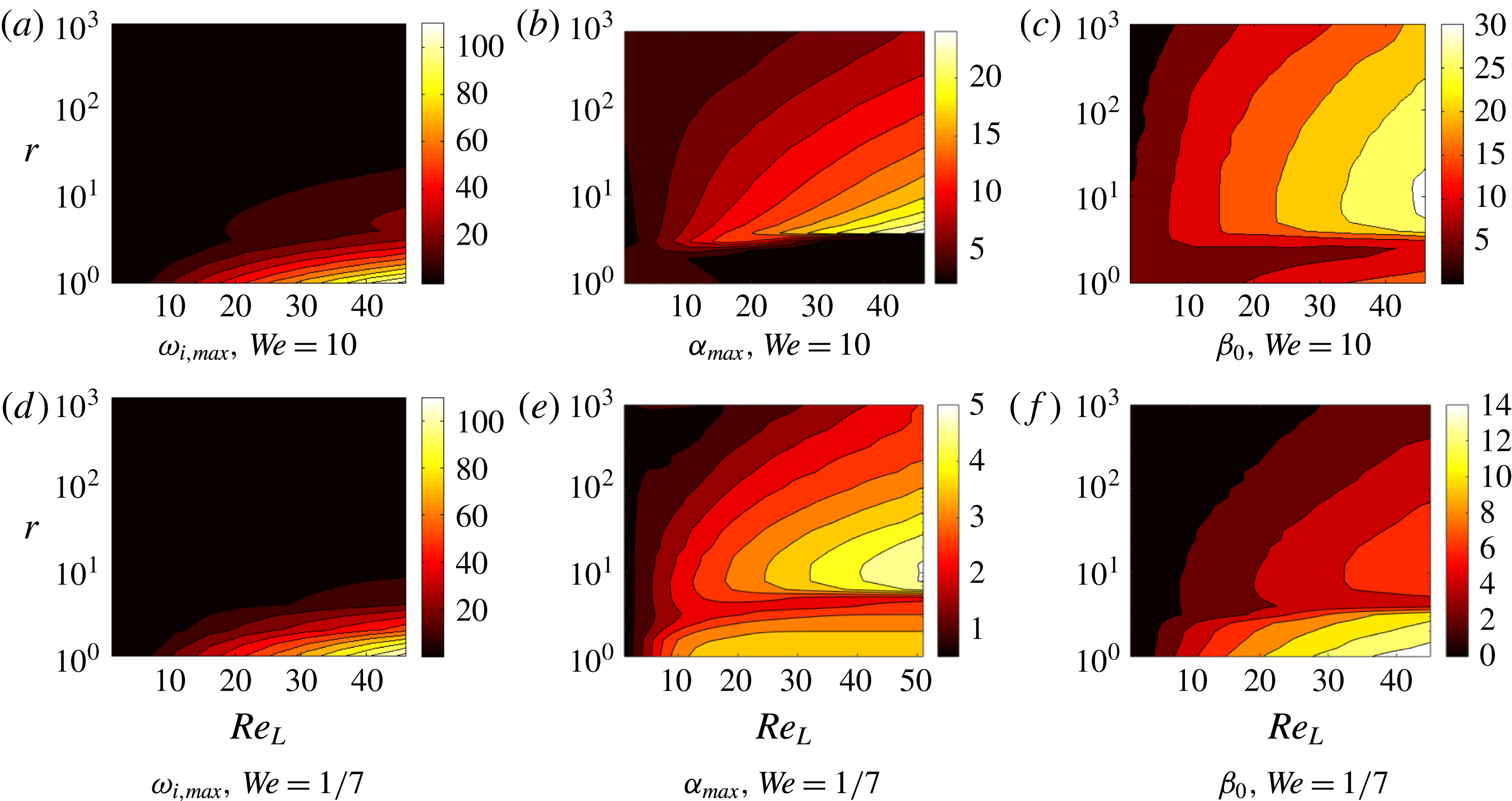
The main trends for both density-matched and density-contrast systems are summarized in figure 3, where the dependence of the maximum growth rate (and other properties) is shown as a function of both
 $r$
and
 $Re$
. Overall, two main trends arise: the growth rate decreases with increasing density ratio, and the cutoff wavenumbers in both streamwise and spanwise directions increase. The picture therefore is one wherein increases in
 $r$
lead to an ever-increasing range of unstable wavenumbers, albeit with diminished growth rates. Additionally, the growth rate of the shear mode increases with Reynolds number; this is in line with shear modes becoming unstable at a critical Reynolds number (e.g. Yiantsios & Higgins Reference Yiantsios and Higgins1988). The same trends persist when the stability analysis is carried out using liquid-layer scaling (figures 4 and 5).
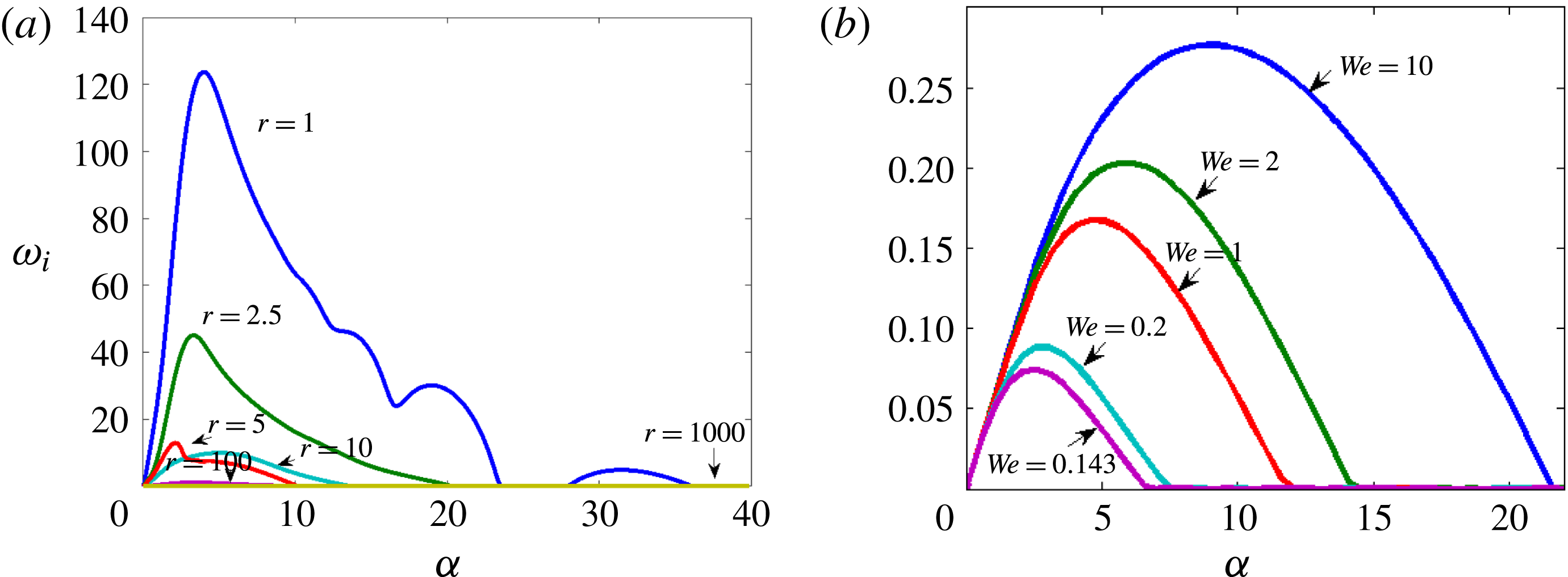
Streamwise-only modal growth rates obtained directly from solving the OSS problem at large surface tension using scaling based on the liquid: (a) for the density ratios indicated, at
 $We=1/7$
and noting that, at
 $r=5$
, there are two unstable modes, only the most dangerous of which is shown; (b) for different values of the Weber number for otherwise the same parameter values, with
 $r=1000$
.

Eigenvalue analysis of the linear system for scaling based on the lower-layer properties for (a–c) weak and (d–f) strong surface tension. The most dangerous mode is always streamwise. (a,d) Maximum (streamwise) growth rate
 $\unicode[STIX]{x1D714}_{i,max}$
; (b,e) the corresponding wavenumber
 $\unicode[STIX]{x1D6FC}_{max}$
; (c,f) the corresponding cutoff spanwise wavenumber
 $\unicode[STIX]{x1D6FD}_{0}$
. The sharp changes below
 $r=10$
arise from mode competition. Other parameters:
 $(m=50,h_{0}=0.2,{\mathcal{G}}_{L}=1)$
.

Two possibilities are suggested as the reason for the decrease in the growth rates with increasing density contrast: either the increase in liquid inertia, or the effect of gravity in the normal stress balance at the perturbed interface. For the ranges of parameter values set out in § 2, we have found that the main effect of the density ratio in the linear stability analysis is the inertial effect; the gravitational term in the normal stress balance only gives a modest effect in our parametric study based on properties of the upper layer at the largest density ratio,
 $r=1000$
. Therefore, the effect of varying the density ratio whilst keeping the fluid properties of either fluid constant may be expected to give similar results for the linear stability analysis. The importance of inertia rather than gravity for stabilizing the interfacial waves carries over to the nonlinear regime also, as described below in § 5.
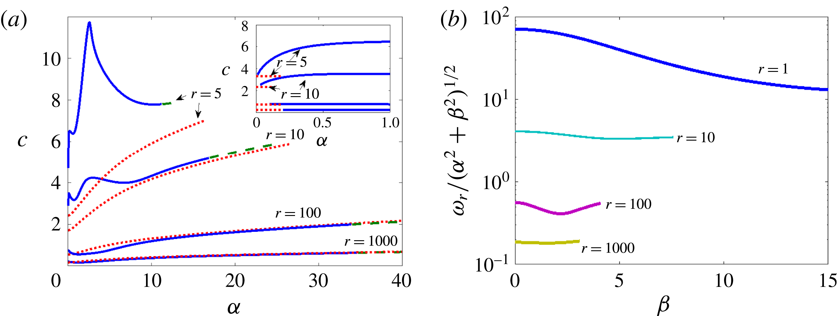
Modal wave speeds for different density ratios
 $r$
obtained directly from solving the Orr–Sommerfeld problem using scaling on liquid properties at large surface tension at
 $(m,h_{0},{\mathcal{G}}_{L},Re_{L},We)=(50,0.2,1,50,1/7)$
. (a) Streamwise-only modal wave speeds; (b) spanwise modal wave speeds as a function of spanwise wavenumber
 $\unicode[STIX]{x1D6FD}$
where
 $\unicode[STIX]{x1D6FC}$
is fixed: for each considered case, the streamwise wavenumber
 $\unicode[STIX]{x1D6FC}$
is the one corresponding to the most dangerous mode. In (a), the broken lines in the main panel represent (4.1), whereas the inset in (a) shows the prediction of the asymptotic formula for the wave speed, valid at
 $\unicode[STIX]{x1D6FC}=0$
.

We elaborate further on the results of the eigenvalue analyses for cases with density contrast. Already at
 $r=5$
the shear mode, seen in the above to dominate at
 $r=1$
, has yielded to the Yih-type mode for the range of cases studied herein (e.g. figure 2
a,b); the same analysis applies when bottom-layer scaling is used (figures 4–6). Although the Yih-type mode initially becomes more unstable when increasing
 $r$
, thereby bucking the general trend, the maximum growth rate diminishes when increasing the density ratio beyond
 $r=10$
(especially when decreasing the gas density for a given liquid).
At large values of
 $r$
, the most unstable mode becomes longer and the growth rate is reduced (see figures 3 and 5). When
 $We$
is decreased, the cutoff streamwise wavenumber (above which the flow is stable) and maximum growth rate are significantly reduced (e.g. figure 4
b), as is normally expected from surface tension. The wave speed of the remaining unstable branch at large
 $r$
is well predicted by inviscid theory for a gravity-capillary wave, given by (Craik Reference Craik1985)
 $$\begin{eqnarray}\displaystyle & \displaystyle c^{2}=\left\{\left({\displaystyle \frac{r-1}{r+1}}\right){\displaystyle \frac{{\mathcal{G}}}{\unicode[STIX]{x1D6FC}}}+{\displaystyle \frac{\unicode[STIX]{x1D6FC}/We}{r+1}}\right\}\text{tanh}(\unicode[STIX]{x1D6FC}h_{0}), & \displaystyle\end{eqnarray}$$
where the wave speed has been made dimensionless with the speed (2.2). This prediction is seen to be accurate at sufficiently large values of
 $r$
in figure 6(a); similar agreement with inviscid theory for the wave speed is also obtained when using a turbulent base flow in the gas (Ó Náraigh et al.
Reference Ó Náraigh, Spelt, Matar and Zaki2011). These modes are unstable due to the Yih mechanism (as demonstrated by energy-budget analysis); thus wave growth is due to viscous effects. The problem of determining the growth rate and departure from (4.1) can be regarded at sufficiently large density ratio as a viscous perturbation of the inviscid gravity-capillary wave – precisely the original premise of the early ‘divide and attack’ approach (Benjamin Reference Benjamin1959). For the flow analysed here, therefore, agreement with (4.1) cannot be used as evidence for an inviscid mechanism governing wave growth.
Three-dimensional modes are not necessarily less unstable in these systems than two-dimensional modes, as discussed in the introduction. Squire’s transformation can be formulated here also, but for Squire’s theorem to apply, increasing the Reynolds number must be destabilizing, which is not necessarily the case throughout parameter space (Yiantsios & Higgins Reference Yiantsios and Higgins1988). Our numerical solution of the stability analysis does show though, for the range of cases considered, that increasing the value of the Reynolds number is destabilizing for fixed values of the other parameters, and that the most unstable mode is streamwise (e.g. figures 3 and 5). These figures also show that the cutoff spanwise wavenumber varies with the density ratio in a similar manner to the cutoff streamwise wavenumber. Therefore, increasing the density ratio increases the range of both streamwise and spanwise unstable wavenumbers.
These three-dimensional modes represent oblique waves that are oriented at an angle
 $\unicode[STIX]{x1D703}=\tan ^{-1}(\unicode[STIX]{x1D6FD}/\unicode[STIX]{x1D6FC})$
to the direction of the applied pressure gradient, so they appear to be longer in the plane of the main flow by a factor
 $1/\cos \unicode[STIX]{x1D703}$
and to move at a phase speed that is larger by the same factor. The phase speed in the plane perpendicular to the wave,
 $\unicode[STIX]{x1D714}_{r}/k$
(where
 $k^{2}=\unicode[STIX]{x1D6FC}^{2}+\unicode[STIX]{x1D6FD}^{2}$
), is found here to be mostly only weakly dependent on
 $\unicode[STIX]{x1D6FD}$
; this is seen in figure 6(b), wherein this phase speed is shown for
 $\unicode[STIX]{x1D6FC}$
set at the most unstable value, at various density ratios. Therefore, the most unstable mode at a given value of
 $\unicode[STIX]{x1D6FD}$
will have the same value of
 $\unicode[STIX]{x1D6FC}$
as the most dangerous streamwise mode, and therefore seem similar in the plane of the main flow, but its real wavenumber
 $k$
is larger and it propagates at a speed in the direction of the wavenumber that can be significantly smaller.
5 Later-stage evolution of two-dimensional waves
Before turning to the full three-dimensional problem, we first investigate the overall system behaviour beyond the small-amplitude scenario and the role of the density ratio therein for two-dimensional systems. For this purpose, we conduct a parametric study and present the various flow regimes in flow-regime maps. The overall system behaviour is characterized, and comparisons are made with the linear theory presented above, although spectral analysis, and a corresponding comparison with linear theory, is deferred until § 6. Throughout this section, the simulations are seeded with the Poiseuille flow profile and pressure drop, and a small-amplitude interfacial perturbation
 $$\begin{eqnarray}\displaystyle & \displaystyle \unicode[STIX]{x1D709}(x,t=0)=h_{0}+{\displaystyle \frac{1}{20}}A_{0}\mathop{\sum }_{n=1}^{20}\cos [n(2\unicode[STIX]{x03C0}/\ell _{x})x+\unicode[STIX]{x1D711}_{n}], & \displaystyle\end{eqnarray}$$
where
 $\unicode[STIX]{x1D711}_{n}\in [0,2\unicode[STIX]{x03C0})$
is a random number and
 $A_{0}=10^{-3}$
is a small amplitude. Although the present small-amplitude initial conditions are not a solution of the OSS equations, after some initial transience they evolve into such a solution. This is confirmed by the simulation results below, and also by prior work in the literature (e.g. Boeck et al.
Reference Boeck, Li, López-Pagés, Yecko and Zaleski2007).
5.1 Flow-regime maps for flows with weak surface tension
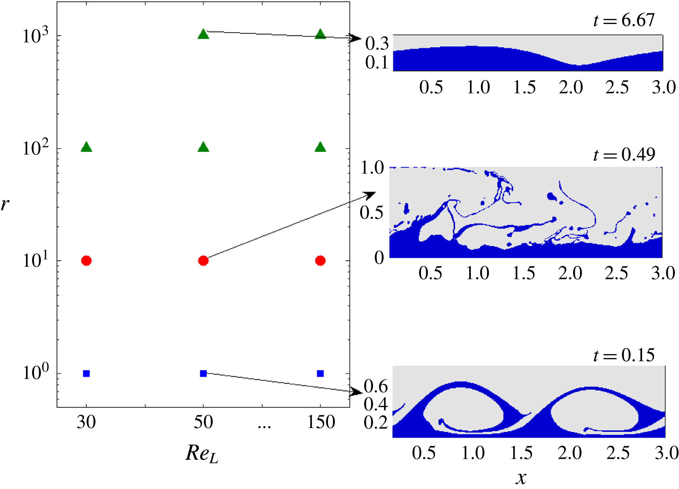
Flow-regime maps are presented in figures 7 and 8 for two different cross-sections of parameter space of systems with weak effects of surface tension, exploring especially the effects of the Reynolds number and density ratio. Although the nonlinear evolution of a purely two-dimensional perturbation is unphysical, the present section plays a key role in the present work – namely to map out the parameter values where different flow regimes occur, by way of a large number of computationally inexpensive two-dimensional simulations. This then pinpoints the parameter values on which to focus in the remaining three-dimensional work. Accordingly, three flow regimes emerge in the region of parameter space scanned, which are discussed here.
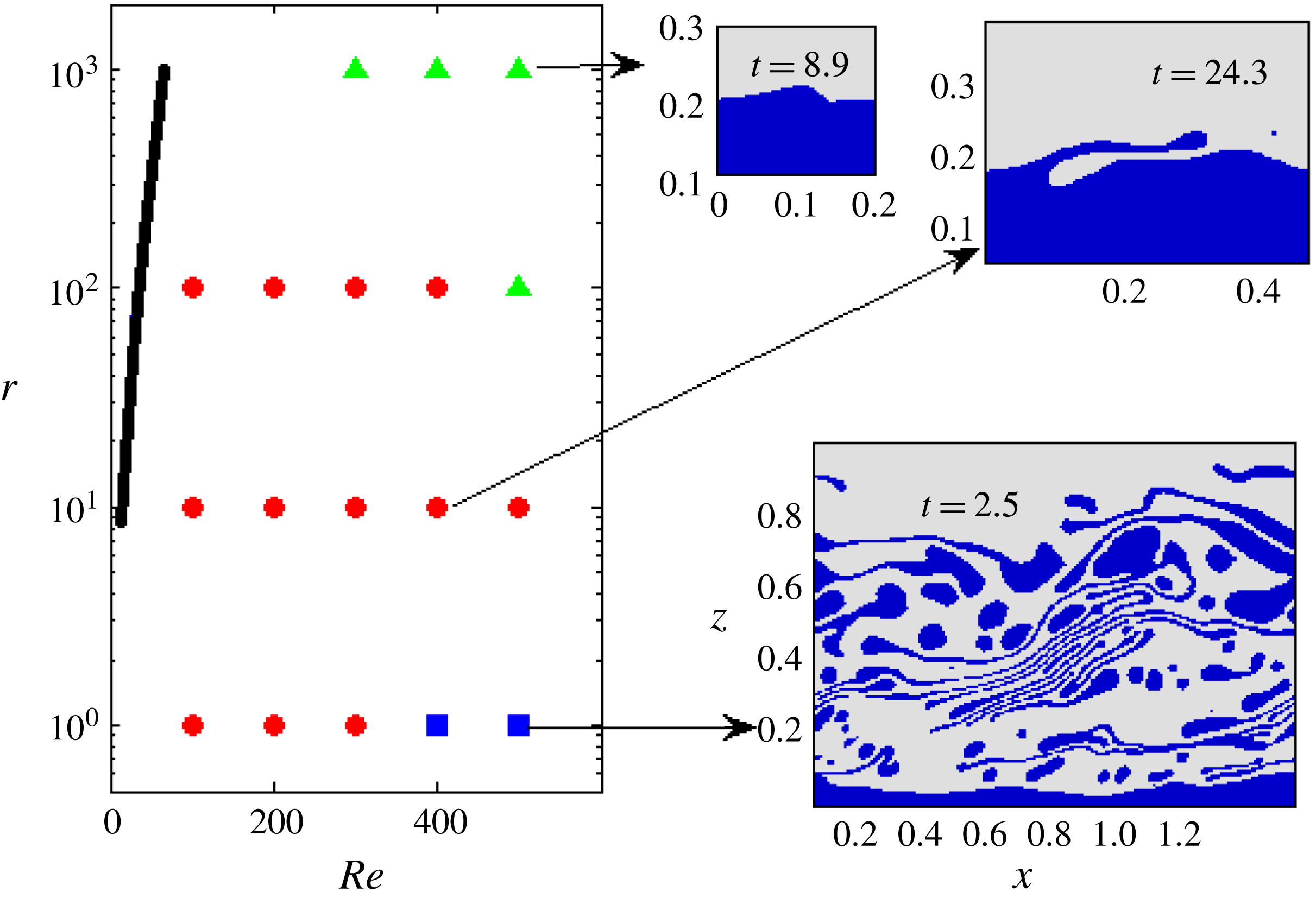
Flow-pattern map for the two-dimensional simulations. The non-dimensionalization is based on the upper-layer properties, with
 $(m=50,h_{0}=0.2,{\mathcal{G}}=0.1,We=10)$
, and such that
 $Re=\unicode[STIX]{x1D70C}_{G}V\ell /\unicode[STIX]{x1D707}_{G}=(\unicode[STIX]{x1D70C}_{G}/\unicode[STIX]{x1D707}_{G})\sqrt{-(\ell /\unicode[STIX]{x1D70C}_{G})(\text{d}p_{0}/\text{d}x)}$
. Symbols: squares, dispersed liquid phase; circles, ligaments; triangles, saturated travelling wave. The insets show snapshots of the three different flow regimes. The top left-hand corner of the main panel is left blank because the growth rates in the linear theory are at least one order of magnitude smaller than in the other parts of the flow-pattern map, meaning that no large-amplitude waves were observed during the course of the numerical simulations. This part of the flow-pattern map is close to the neutral curve (a portion of which is shown here as a solid line) indicating the stability boundary according to linear (eigenvalue) theory.

Flow-pattern map for the two-dimensional simulations based on lower-layer scaling. The simulations use
 $\ell _{x}=3$
. Other parameters:
 $(m=50,h_{0}=0.2,{\mathcal{G}}_{L}=1,We=10)$
. Symbols: squares, dispersed liquid phase; circles, ligaments. The insets show snapshots of the three different flow regimes.

We first consider varying the density ratio for a range of values of
 $Re$
using the upper-layer properties; a flow diagram in a cross-section of parameter space (
 $r,Re$
) is presented in figure 7 for
 $(m=50,h_{0}=0.2,{\mathcal{G}}=0.1,We=10)$
. In this cross-section, a larger value of
 $r$
corresponds to a heavier liquid for a given gas; varying
 $r$
at a given
 $Re$
does not change a Reynolds number based on the superficial gas velocity whereas that for the liquid is reduced inversely proportionally with
 $r$
; the cases studied span
 $348\leqslant Re_{SG}\leqslant 8692$
, with
 $9\leqslant Re_{SL}\leqslant 212$
for
 $r=1000$
.
For very high density contrast (
 $r=1000$
), under these conditions, linear theory is shown in § 4 to predict waves moving at a speed described well by inviscid theory that are unstable due to the Yih mechanism. These are seen here to saturate into finite-amplitude travelling waves. The waves are stabilized largely by inertia (as opposed to gravity), as performing the same simulations again with
 ${\mathcal{G}}=0$
produces qualitatively the same picture.
In contrast, for low density ratios and high Reynolds numbers, for which linear theory in § 4 predicts dominance of shear modes, a large-amplitude wave forms (fed by the linear instability) that engulfs the entire gas phase. Similar large billows have been observed in sheared identical fluids wherein an asymmetry was introduced through the initial velocity profile, which was constant velocity in the two fluids with a boundary layer profile in the upper fluid (Boeck et al.
Reference Boeck, Li, López-Pagés, Yecko and Zaleski2007). Without this boundary layer, this behaviour was not observed in that prior work, consistent with the present finding of a shear mode being at the root of this instability. This behaviour was not observed in Ó Náraigh et al. (Reference Ó Náraigh, Valluri, Scott, Bethune and Spelt2014); although the Reynolds and Weber numbers were varied in that study, the viscosity ratio and the depth ratio of the two layers were kept constant at
 $m=30$
and
 $h_{0}=0.3$
, respectively, different from the values used herein (we return to this in the next section). These waves ‘roll up’ and a complicated structure forms, the eventual result of which is a liquid phase that is dispersed throughout the gas phase, as shown in figure 7 (inset, bottom right). Although the liquid breakup and dispersion in figure 7 is the result of numerical rupture, such simulations are known to capture the basic features of the flow quite well (Scardovelli & Zaleski Reference Scardovelli and Zaleski1999). For this reason the late-time images in figure 7 are included here without further elaboration.
At low to intermediate density ratios, again dominated by the Yih mode in linear stability theory (see § 4), a regime is observed that can be thought of as a balance between the two former regimes. Here, a ligament flow regime emerges, whereby ligaments are constantly entrained into the gas phase. The flow is qualitatively similar to that observed in sheared two-layer flows with moderate density contrast (e.g. Boeck et al. Reference Boeck, Li, López-Pagés, Yecko and Zaleski2007), although here waves turn over towards the interface, such that an intermediate zone between the liquid film and the gas stream exists, comprising a complicated mixture of liquid ligaments and gas pockets. The corresponding simulations were performed such that many iterations of ligament formation and turnover were observed, such that an eventual steady state devoid of ligaments is ruled out, meaning that the structures observed in figure 7 represent a long-time (quasi-steady) state.
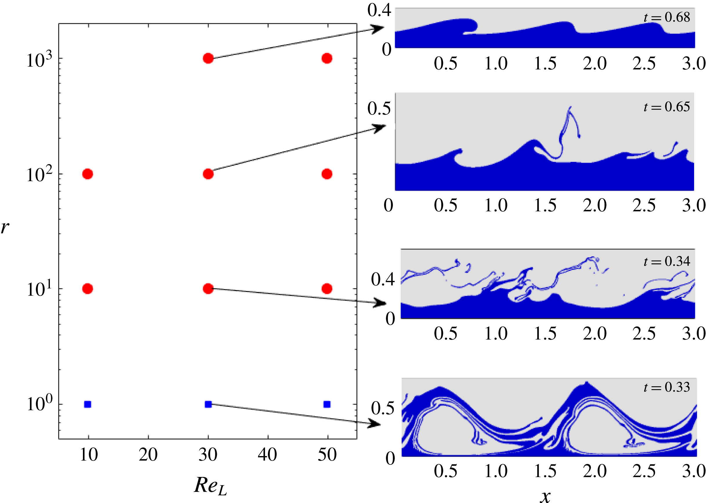
Flow-pattern map for the two-dimensional simulations based on lower-layer scaling – large surface tension. The simulations use
 $\ell _{x}=3$
. Other parameters:
 $(m=50,h_{0}=0.2,{\mathcal{G}}_{L}=1,We=1/7)$
. Symbols: squares, dispersed liquid phase; circles, ligaments; triangles, saturated travelling wave. The insets show snapshots of the three different flow regimes.

To verify the robustness of the conclusions drawn above, we now investigate the effects of density ratio using a different cross-section in parameter space, by adopting scaling based on the liquid properties, i.e. based on (2.4), such that a larger density ratio corresponds now to a reduction in gas density. In this cross-section of parameter space, a Reynolds number based on the superficial gas velocity now varies inversely proportionally with
 $r$
at a given
 $Re_{L}$
, whereas that for the liquid remains constant; the ranges spanned by the axes correspond to
 $0.21\leqslant Re_{SL}\leqslant 5.3$
, with
 $8.7\leqslant Re_{SG}\leqslant 217$
for
 $r=1000$
. The results of modal linear theory were found in § 4 similar to those obtained when using scaling on the gas properties, but with much reduced growth rates at large density ratios. The corresponding results in the nonlinear regime are shown in the flow-pattern map in figure 8. Overall, the flow-pattern map is similar to the one based on upper-layer scaling, with significant regions that admit both a dispersed phase and a ligament phase, whereas saturated waves were not observed in this range of cases. Ligaments are observed at up to
 $r=1000$
, while the dispersed phase is seen clearly again to be the result of the rollup of a large-amplitude wave.
5.2 Effects of surface tension on flow regimes
The flow-regime maps presented thus far are for weak surface tension. In figure 9 we present the flow regime map for the same cross-section in parameter space as figure 8, but at the much lower Weber number,
 $We=1/7$
.
It was already noted in § 4 that the linear shear modes that dominate for the density-matched cases studied here are not sensitive to surface tension. This is now seen to extend to the nonlinear regime: the flow regime for density-matched fluids is still rollup. At very large density ratio (
 $r=1000$
), a quasi-steady long saturated wave is now obtained, instead of a ligament. As in the parametric study presented in figure 8, inertial effects of the gas are reduced here, since
 $Re_{SL}$
is reduced when
 $r$
is increased. The sole difference between these is that surface tension is now much stronger, which is therefore the cause of the saturation of the wave. If the effects of the gas flow are ignored entirely, the problem setup becomes similar to that of a film falling down a plane under an angle
 $\tan ^{-1}({\mathcal{G}}_{L})$
. The observed shape of the saturated wave shows some resemblance to that observed – for instance, see figure 3 in Charogiannis et al. (Reference Charogiannis, Denner, van Wachem, Kalliadasis and Markides2017). This suggests that an approach based on low-dimensional modelling (Ruyer-Quil & Manneville Reference Ruyer-Quil and Manneville2000) may be feasible here.
Formation and subsequent collapse of a huge wave at large density ratio and large surface tension
 $(r=100,m=50,h_{0}=0.2,Re_{L}=50,{\mathcal{G}}_{L}=1,We=1/7)$
.

(a) Averaged velocity in the entire unit cell versus time for the huge wave (parameters
 $r=100,m=50,h_{0}=0.2,Re_{L}=50,{\mathcal{G}}_{L}=1,We=1/7$
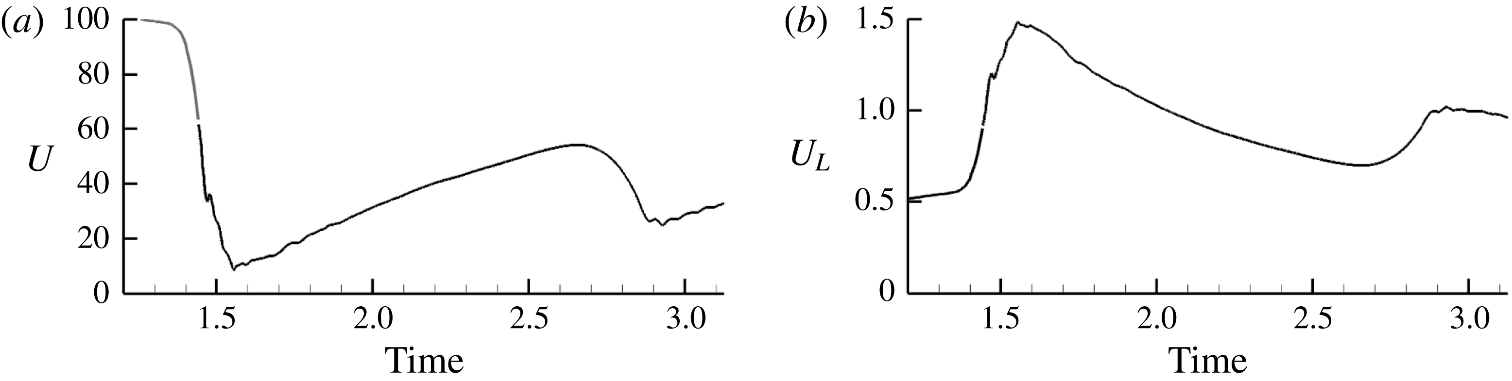
; figure 10). (b) Superficial liquid velocity versus time for the same case. The drop in the flow rate in (a) is seen to correspond to the formation of the huge wave in figure 10.

At
 $r=100$
, the flow behaviour is also rather different from that observed in the low-surface-tension case: a very large wave may be formed rapidly, which collapses into waves of saturated amplitude at long times, shown in figure 10. The huge wave, formed after coalescence of smaller waves, leaves only a thin liquid film at its trough. This behaviour was observed at low to moderate Reynolds number, but not at the largest Reynolds number simulated. The final collapse of the huge wave was found not to be the result of gravity; simulations without and with gravity (at
 $Re_{L}=30$
,
 $r=100$
) showed the same behaviour. Stabilization by surface tension is overcome by the destabilizing flow; in the simulation, however, the pressure drop over the unit cell is kept fixed, not the flow rate. By the time a large wave has formed, the total flow rate has reduced significantly; for the case shown in figure 10, by almost an order of magnitude (the time evolution of the flow rates is shown in figure 11). After the wave collapse, the flow accelerates again. The formation of these huge waves can therefore be of significance even though they collapse eventually if the pressure drop is kept constant. Finally, for
 $r=1$
and
 $r=10$
the flow in the high-surface-tension case is qualitatively similar to that observed previously for low surface tension (e.g. figure 8).
5.3 Persistence of linear theory: vorticity field
Thus far, we have considered the evolution of the wave shape; we now investigate the associated flow behaviour. In particular, we are interested in whether the mechanism of wave growth identified in linear theory persists.
Isocontours of the perturbation vorticity field for
 $(r=10,m=50,h_{0}=0.2,Re_{L}=30,{\mathcal{G}}_{L}=1,We=1/7)$
. The vorticity component shown is defined in the direction coming out of the plane (
 $=-\unicode[STIX]{x1D714}_{y}$
). The colour range for the liquid vorticity has been adapted, and the contours near the interface have been suppressed, as explained in the main text.

The manner whereby streamwise Yih modes gain energy from the base flow under linear theory has been reasoned out in Boomkamp & Miesen (Reference Boomkamp and Miesen1996), but in terms of an energy budget. The analysis of the mechanism in Hinch (Reference Hinch1984) of flows with weak inertia (Hooper & Boyd Reference Hooper and Boyd1983) is of interest here, as an energy budget of these flows was found to be similar to Yih modes (Boomkamp & Miesen Reference Boomkamp and Miesen1996). Motivated by the mechanism identified in Hinch (Reference Hinch1984), and prior work on wave growth on falling films (Kelly et al. Reference Kelly, Goussis, Lin and Hsu1989), we investigate the perturbation vorticity field, and whether this is out of phase with the wave.
We recall that the mechanism proposed in Hinch (Reference Hinch1984) arises from the discontinuity in shear rate that appears in an unperturbed unidirectional parallel shear flow of two fluids. Introduction of a perturbation of the interface whereat the velocity is continuous then creates vorticity at the interface in each fluid, and this diffuses by viscosity away from the interface, and is advected downstream by inertia, which causes a phase difference with the interface. This occurs in each fluid similarly and would therefore not result in wave growth, were it not that the vorticity created at the interface is larger in the less viscous fluid, in lieu of the continuity of tangential stress. The motion associated with this dominant vorticity in the less viscous fluid, diffused and advected somewhat away from its origin at the interface, is found to be consistent with growth of the wave amplitude.
To investigate the relevance of this mechanism in the present system, and the perturbation of the vorticity field not being large in comparison with unperturbed vorticity, we present a time sequence for the difference between instantaneous and initial vorticity field in figure 12. The mere occurrence of wave growth trivially introduces a strong perturbation in this perturbation field, as the liquid under a wave crest was previously occupied by the gas and vice versa above a wave trough, which would obscure the presentation. In figure 12, we have therefore set the perturbation field to zero in a band around the initial interface location and around the actual interface location. Because of the continuity of tangential stress at an interface, as mentioned above, the vorticity in the (more viscous) liquid is much weaker than in the gas; the colour range in figure 12 for the perturbation vorticity in the liquid has been adapted for presentational reasons. The wave evolution is therefore expected to be associated mostly with the vorticity in the (less viscous) gas phase (Hinch Reference Hinch1984).
The perturbation vorticity field shown in figure 12(a) corresponds to an increase (decrease) in
 $\unicode[STIX]{x1D714}_{y}$
around a wave crest (trough), with distortion due to advection. (In the present context, it is natural to use the symbol
 $\unicode[STIX]{x1D714}_{y}$
for the
 $y$
component of the vorticity, such that the previous association of that symbol with the eigenfrequency of the linear stability analysis is suspended for the present purpose.) These observations are consistent with the mechanism for instability identified by Hinch (Reference Hinch1984) (noting that he took the lower fluid as the less viscous).
The later wave evolution, presented in figure 12(b,c), confirms that the disturbance vorticity field is still seen to be qualitatively similar, although disturbances of shorter wavelength appear; eventually this leads to shedding of vorticity from the wave crest that is observed also in sheared two-layer flows at moderate density ratio (Boeck et al. Reference Boeck, Li, López-Pagés, Yecko and Zaleski2007).
6 Later-stage evolution of three-dimensional waves
In the following, we first study the evolution of three-dimensional perturbations for a broad range of density ratios by DNS. The simulations are seeded with the Poiseuille flow profile and pressure drop, and a small-amplitude interfacial perturbation
 $$\begin{eqnarray}\displaystyle & \displaystyle \unicode[STIX]{x1D709}(x,y,t=0)=h_{0}+{\displaystyle \frac{1}{16}}A_{0}\mathop{\sum }_{m=0}^{3}\mathop{\sum }_{n=0}^{3}\cos [(2\unicode[STIX]{x03C0}/\ell _{x})mx+(2\unicode[STIX]{x03C0}/\ell _{y})ny+\unicode[STIX]{x1D711}_{mn}], & \displaystyle\end{eqnarray}$$
where
 $\unicode[STIX]{x1D711}_{mn}\in [0,2\unicode[STIX]{x03C0})$
is a random number and
 $A_{0}=5\times 10^{-3}$
is a small amplitude. The amplitude corresponds to a root-mean-square interface disturbance
 $[\overline{(\unicode[STIX]{x1D709}-h_{0})^{2}}]^{1/2}=\sqrt{2}A_{0}/16$
, hence
 $[\overline{(\unicode[STIX]{x1D709}-h_{0})^{2}}]^{1/2}/h_{0}=0.22\,\%$
for
 $h_{0}=0.2$
, i.e. a perturbation less than 1 % of the mean wave height. This initialization is similar to the corresponding version in two dimensions (e.g. equation (6.1)). It is also very similar to the methodology in our earlier works on density-matched systems (Valluri et al.
Reference Valluri, Ó Náraigh, Ding and Spelt2010; Ó Náraigh et al.
Reference Ó Náraigh, Valluri, Scott, Bethune and Spelt2014), albeit that the purely spanwise modes (i.e.
 $m=0,n\neq 0$
) are treated slightly differently in the present case. Nevertheless, a comparison between the present gas–liquid work and our earlier liquid–liquid studies is still possible.
The aim of the present section is to compare the behaviour of the three-dimensional waves to the flow-regime maps presented in the previous section for purely two-dimensional flows. Furthermore, the results are compared with prior work on three-dimensional nonlinear wave evolution in density-matched systems (Ó Náraigh et al. Reference Ó Náraigh, Valluri, Scott, Bethune and Spelt2014). As such, the strategy of the parametric study in this section is to identify key typical cases from the two-dimensional flow-pattern maps in § 5, and to perform corresponding three-dimensional simulations. The identified cases are strongly supercritical, meaning that modal eigenvalue analysis is expected at early times. The corresponding late-time behaviour should then be largely independent of the initial conditions, as the most unstable eigenmode will be selected. This is in contrast to subcritical scenarios (e.g. in the theory of transition to turbulence), where not only the initial conditions, but also the boundary conditions are important (Buffat et al. Reference Buffat, Le Penven, Cadiou and Montagnier2014).
6.1 Flow behaviour and comparison with linear theory
We shall refer to the parameters
 $(m=50,h_{0}=0.2,{\mathcal{G}}=0.1,We=10)$
with scaling on the gas properties as the basis configuration; we recall that the corresponding flow-regime map for two-dimensional flows is in figure 7.
6.1.1 Density-matched systems
These have been considered in prior work (Ó Náraigh et al.
Reference Ó Náraigh, Valluri, Scott, Bethune and Spelt2014), but we revisit them here, to develop a ‘base case’ relative to which other simulations with a density contrast can be compared, which is at
 $m=50$
,
 $h_{0}=0.2$
. The basis configuration at
 $r=1$
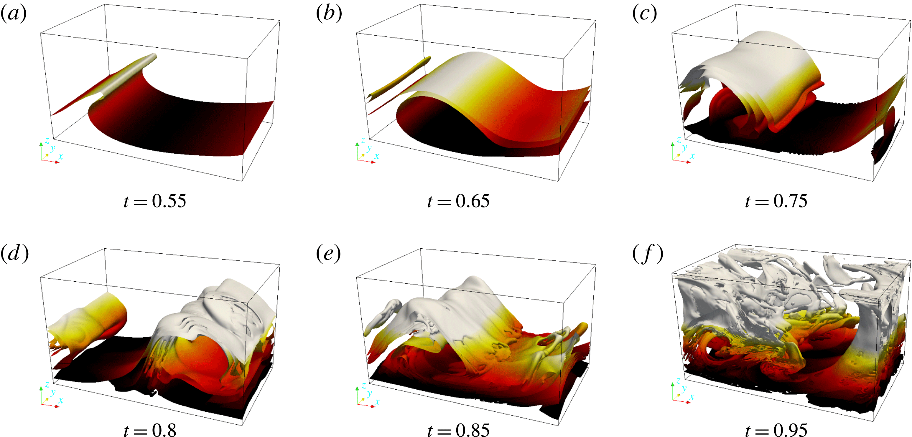
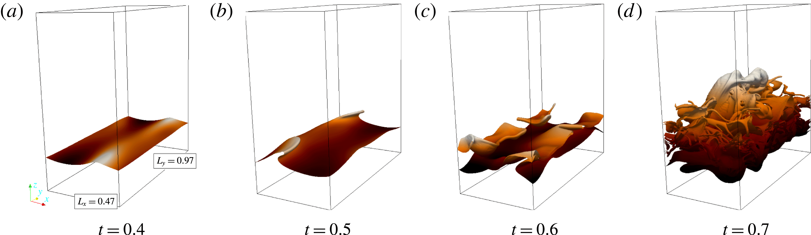
can be thought of as ‘barely supercritical’, with a single unstable streamwise mode fitting inside the simulation domain and all other modes stable, and we recall that the most dangerous mode in linear theory in this instance is a shear mode. The striking flow behaviour observed for this case (see figure 13) is much more two-dimensional in nature than that in the cases simulated in Ó Náraigh et al. (Reference Ó Náraigh, Valluri, Scott, Bethune and Spelt2014), besides exhibiting billows of larger amplitude. In that work, results were presented for several values of the Reynolds and Weber numbers (notably,
 $Re\leqslant 100$
), while the viscosity ratio was fixed at
 $m=30$
and the dimensionless height at
 $h_{0}=0.3$
(we take this opportunity to correct the definition of the parameter
 ${\mathcal{S}}$
in that study, which in fact is
 $1/We$
), which are not suitable for the present purposes. Linear stability analysis reveals that an important effect of moving to the present set of parameter values is that the increase in the selected Reynolds number increases the maximum growth rate, thereby providing an energy source for the huge billows observed in the present work.
Interface shape evolution from DNS for a three-dimensional density-matched system. Parameters
 $(r=1,m=50,h_{0}=0.2,We=10)$
, and
 $Re=500$
.

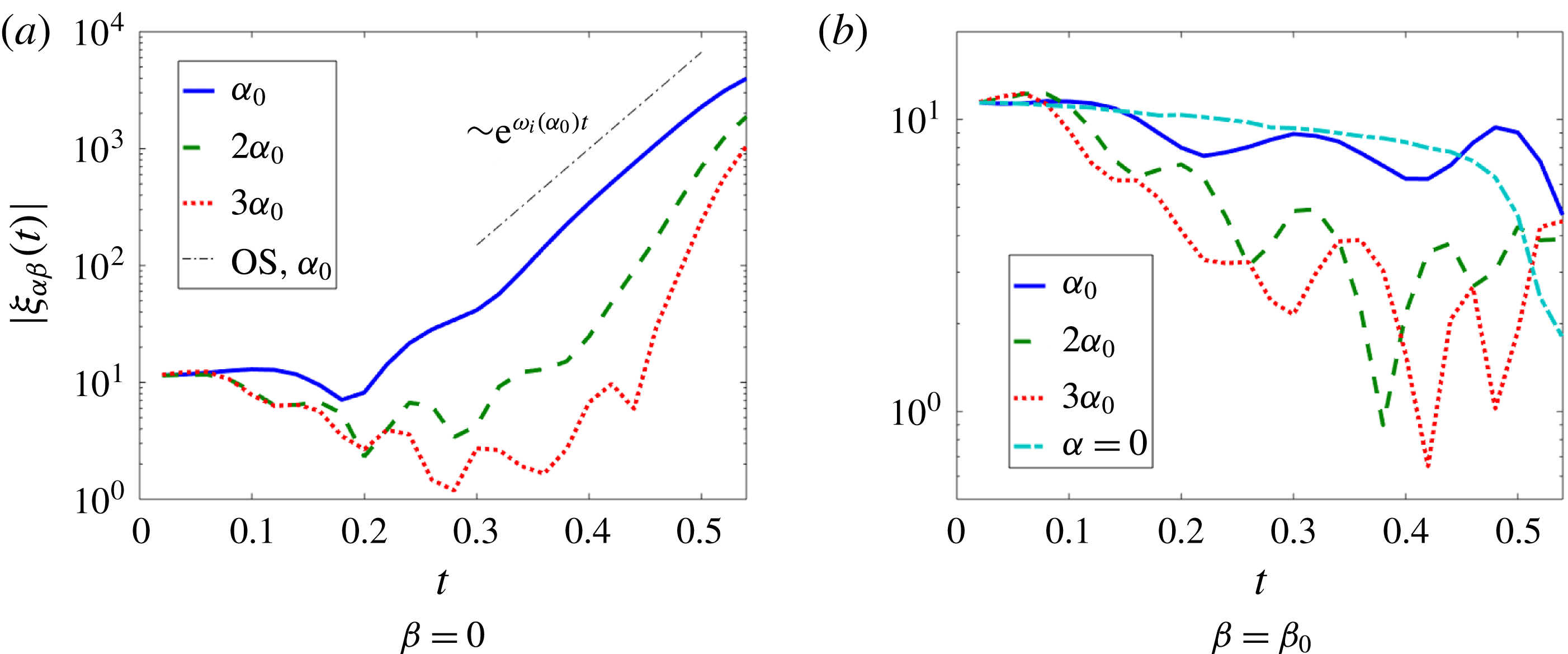
To understand the results of figure 13 in more depth, a spectral analysis of the various modes is presented in figure 14. The analysis is based on interfacial spectra
 $\unicode[STIX]{x1D709}_{\unicode[STIX]{x1D6FC}\unicode[STIX]{x1D6FD}}(t)$
, where
 $$\begin{eqnarray}\displaystyle & \displaystyle \unicode[STIX]{x1D709}_{\unicode[STIX]{x1D6FC}\unicode[STIX]{x1D6FD}}(t)=\int _{0}^{\ell _{x}}\text{d}x\int _{0}^{\ell _{y}}\text{d}y\,\unicode[STIX]{x1D709}(x,y,t)\text{e}^{-\text{i}\unicode[STIX]{x1D6FC}x-\text{i}\unicode[STIX]{x1D6FD}y}. & \displaystyle\end{eqnarray}$$
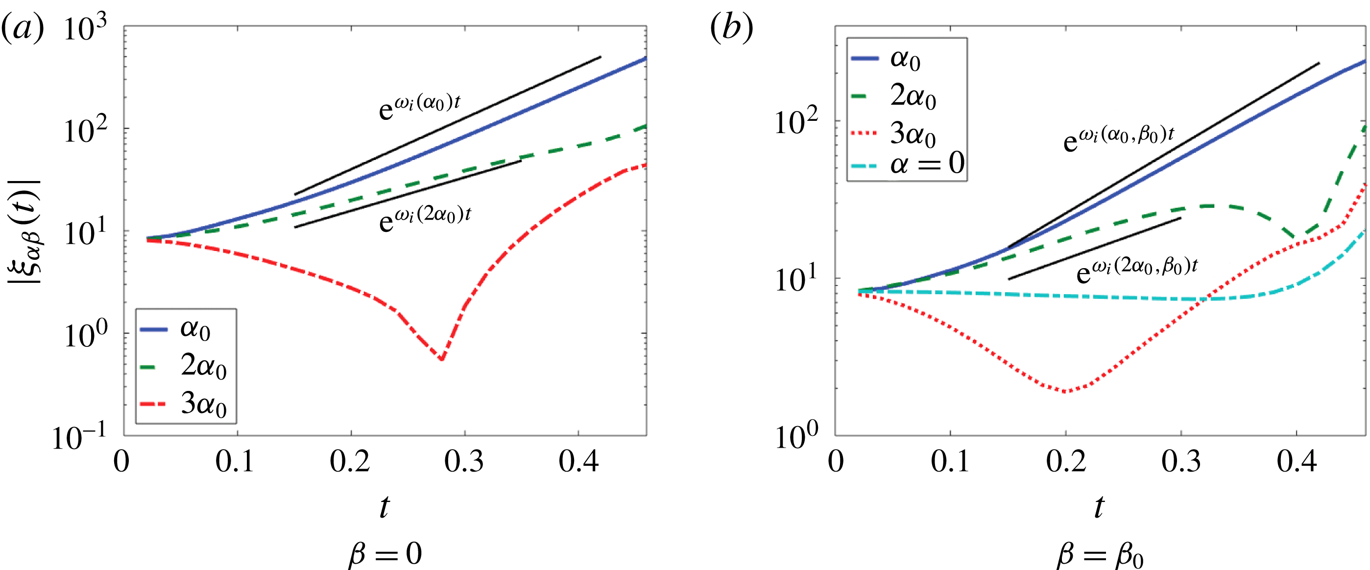
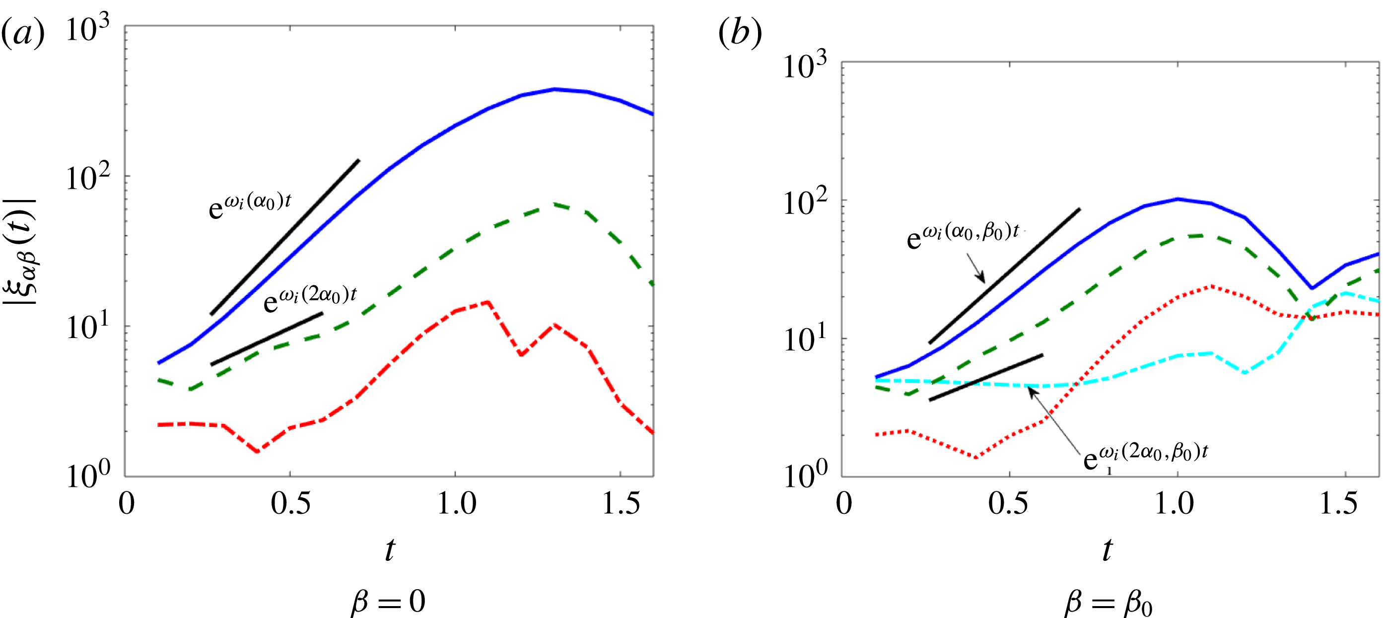
The analysis demonstrates that eigenvalue linear theory here holds up until the advent of wave overturning for the streamwise unstable mode (the ‘fundamental’ mode with
 $\unicode[STIX]{x1D6FC}=2\unicode[STIX]{x03C0}/\ell _{x}$
) and the spanwise modes, as in the cases considered in Ó Náraigh et al. (Reference Ó Náraigh, Valluri, Scott, Bethune and Spelt2014). Also, the overtones of the fundamental streamwise mode appear to be slaved to the fundamental itself according to weakly nonlinear theory. Purely spanwise modes are not amplified strongly in the present case, unlike in the otherwise similar density-matched cases studied in Ó Náraigh et al. (Reference Ó Náraigh, Valluri, Scott, Bethune and Spelt2014). This difference is due in part to the difference in how the purely spanwise modes are triggered in the two studies – purely spanwise modes have the same initial amplitude as all the other modes in the present work, whereas in the prior work they had a smaller amplitude. In any case, the duration of the weakly nonlinear regime is short in the present case (due to the early onset of the strongly nonlinear regime with wave overturning, ligament formation, etc.). As the strongly nonlinear regime is therefore more dominant and more robust to different choices of initial conditions, this small difference is not investigated in the present work.
Spectral analysis of DNS results for a density-matched system that evolves into large, mostly two-dimensional billows (see also figure 13). Other parameters
 $(m=50,h_{0}=0.2,{\mathcal{G}}=0.1,We=10)$
, and
 $Re=500$
. Here,
 $\unicode[STIX]{x1D6FC}_{0}=2\unicode[STIX]{x03C0}/\ell _{x}$
and
 $\unicode[STIX]{x1D6FD}_{0}=2\unicode[STIX]{x03C0}/\ell _{y}$
denote the fundamental wavenumber in the streamwise and spanwise directions, respectively.

A further departure from two-dimensional flow may be expected at larger Reynolds numbers, where more three-dimensional modes become linearly unstable. For density-matched systems, such ‘supercritical’ cases have been studied in Ó Náraigh et al. (Reference Ó Náraigh, Valluri, Scott, Bethune and Spelt2014). Three-dimensional modes grow in accord with linear theory, but purely spanwise modes are again amplified by the same weakly nonlinear mechanism, due to properties of the dispersion relation. For the present basis configuration of density-matched fluids, Reynolds numbers were not increased further due to computational limitations.
As in the flow-pattern map (see figure 7, lower inset), the sheets roll up in the streamwise direction (figure 13 b), although now three-dimensional waves form on the sheet (figure 13 c) resulting in a final state comprising a complex three-dimensional dispersed phase (figure 13 f). Similar to the two-dimensional case, details of the interfacial structure at late time in figure 13 may not be fully resolved, but the same qualitative features of the interface persist when simulations at higher resolution are performed. Therefore, following Scardovelli & Zaleski (Reference Scardovelli and Zaleski1999) we view such simulations as giving a good qualitative picture of the interface behaviour at late times.
6.1.2 Moderate density ratio
In the preceding sections the Yih instability mechanism has been found to be dominant for linear growth for the cases considered wherein the densities are not matched, and ligament growth is observed in two-dimensional simulations. A spectral analysis is presented for the three-dimensional flow of the basis configuration in figure 15. Here also, linear theory holds up nearly until the waves overturn for both streamwise and spanwise modes. As a broad spectrum of streamwise and spanwise waves are linearly unstable, three-dimensional waves are promoted directly via linear theory.
Spectral analysis of DNS results at a moderate density ratio,
 $r=10$
, accompanying figure 16. Other parameters
 $(m=50,h_{0}=0.2,{\mathcal{G}}=0.1,We=10)$
, and
 $Re=500$
; values
 $\unicode[STIX]{x1D6FC}_{0}=2\unicode[STIX]{x03C0}/\ell _{x}$
and
 $\unicode[STIX]{x1D6FD}_{0}=2\unicode[STIX]{x03C0}/\ell _{y}$
denote the fundamental wavenumber in the streamwise and spanwise directions, respectively.

Interface shape evolution from DNS for a case at moderate density ratio,
 $r=10$
. Other parameters:
 $(m=50,h_{0}=0.2,{\mathcal{G}}=0.1,We=10)$
, and
 $Re=500$
.

Liquid sheets form at the crests of the unstable waves at the point of wave overturning as in the density-matched case (figure 16
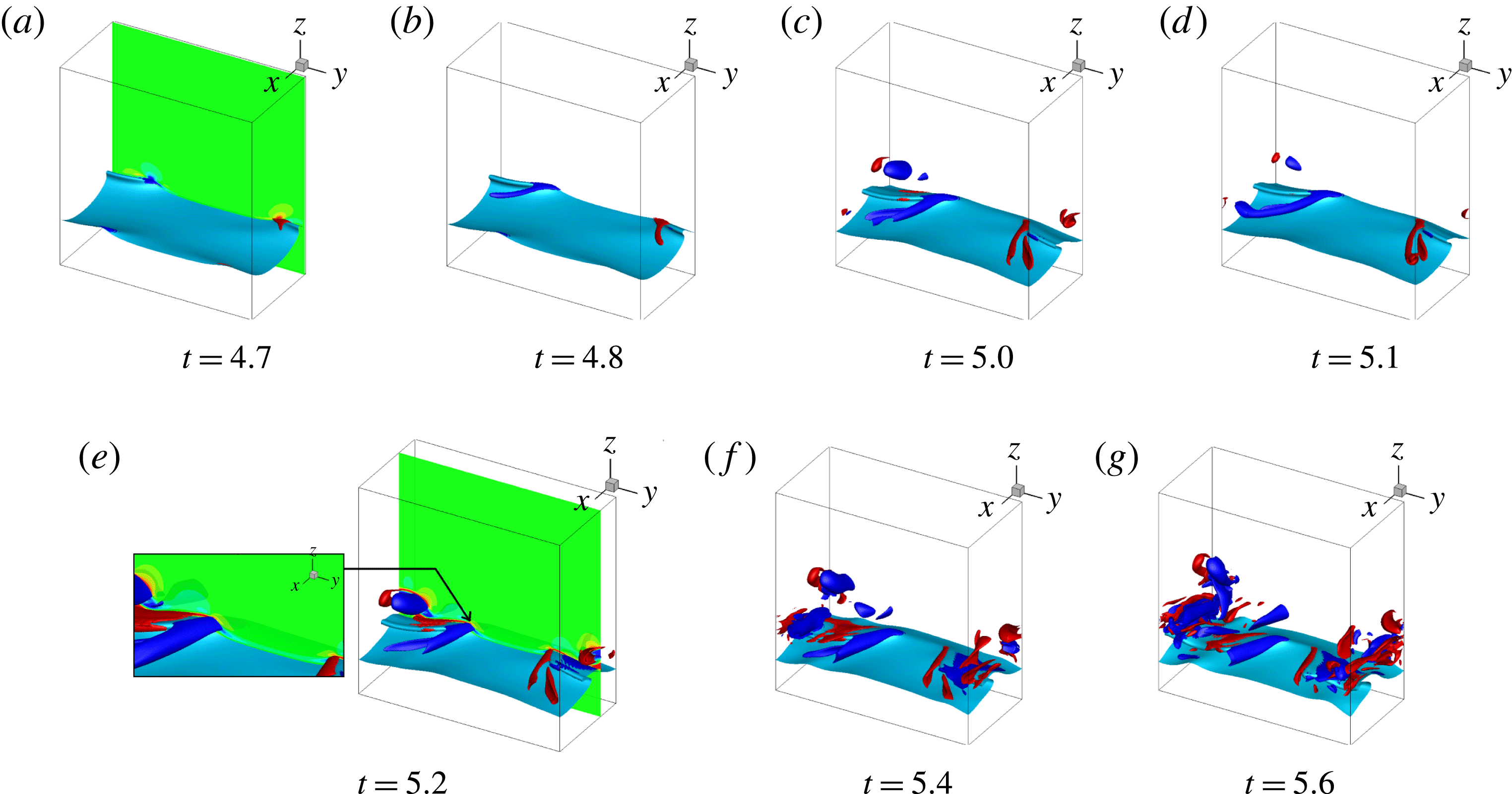
b). However, the sheets now exhibit a strong spanwise modulation. The same modulation produces spanwise variations in the pressure and velocity fields (including a strong cross-stream velocity component), which further distort the sheets. In this way, fully three-dimensional oblate ligaments form that are further elongated by the mean flow. At later times, the tip of the ligament is drawn upwards such that the liquid sheet on the upwind side forms a depression and a bowl-like structure emerges, which is entrained higher into the gas layer (figure 16
c). This entrainment continues indefinitely, such that the final state is a dispersed mixture that fully extends into the gas domain and sits on top of a thin continuous liquid film (figure 16
d). Again, this outcome corresponds to a first approximation to the predicted flow regime of the two-dimensional flow-pattern map: the flow-pattern map predicts ligament growth for
 $r=10$
and
 $Re=500$
– see figure 7.
The results of simulations when scaling on the liquid properties, corresponding to the flow diagram (figure 8), are essentially the same, as the two flow-regime maps coincide at
 $r=10$
. Results for bottom-layer scaling are reported in figure 17(a,b), also to provide comparison with results for a larger density ratio considered next. As the results based on both upper-layer and lower-layer scaling agree qualitatively, it suffices to provide the detailed spectral analysis for the former.
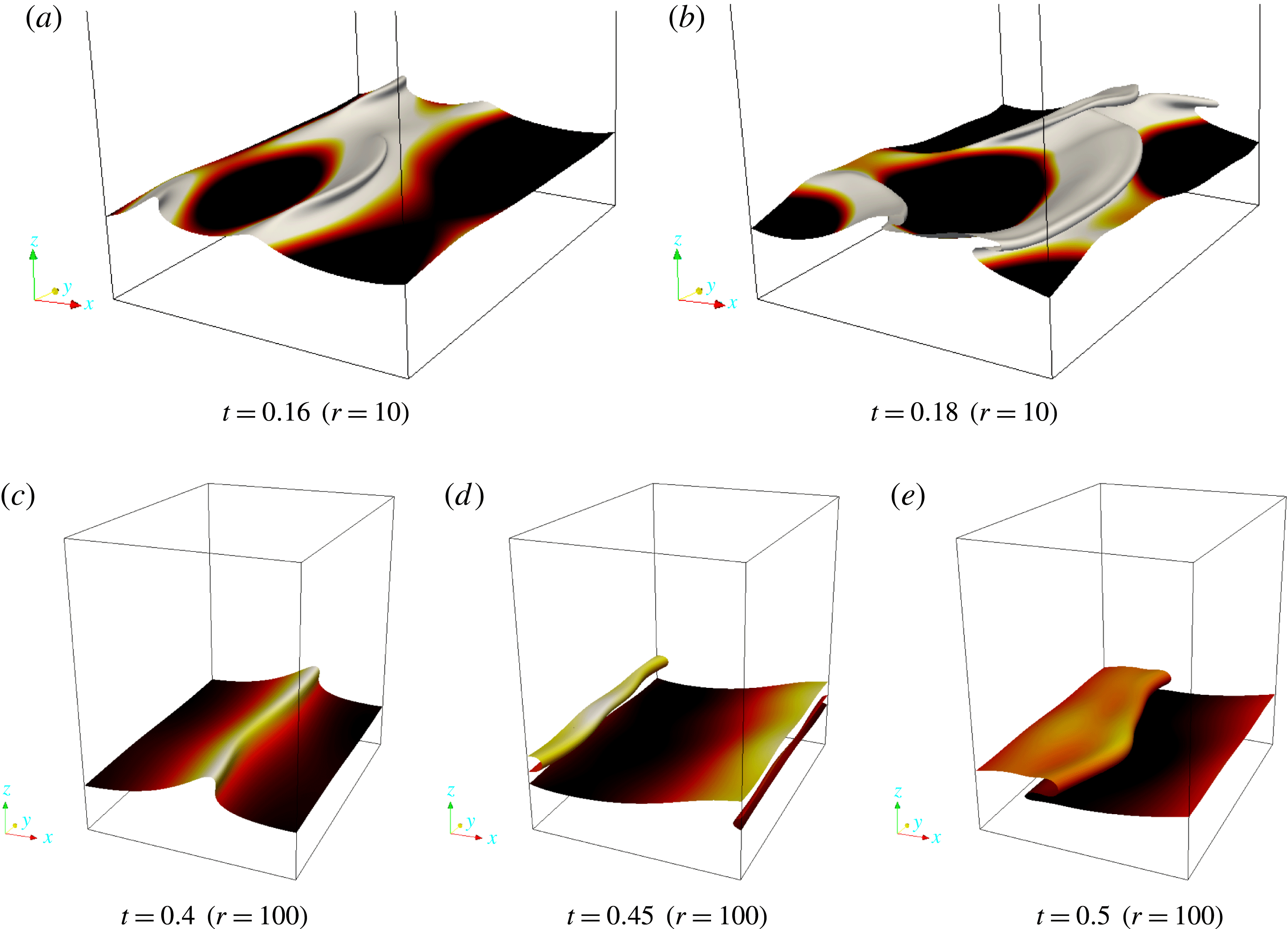
DNS results for liquid-layer scaling with
 $h=0.2,~m=50,~Re_{L}=30,~{\mathcal{G}}_{L}=1$
, and
 $We=10$
. Panels show capillary ridge formation at large density ratio and comparatively low Reynolds number, for (a,b)
 $r=10$
and (c–e)
 $r=100$
.

6.1.3 High density ratios
For
 $r=100,1000$
, the growth rate predicted by linear theory is found to be much reduced compared to previous cases with
 $r=1,10$
(in short, the wave speed at
 $r=100,1000$
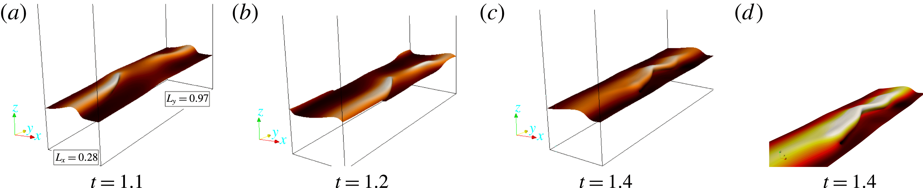
is found to be governed by inviscid theory, while the growth rate is associated with the Yih instability). Correspondingly, in the DNS we find that the ligaments observed at the lower density ratios are much suppressed, and the interface is stabilized with respect to the ‘bowl breakup’ mentioned above. In this way, quasi-two-dimensional travelling waves emerge at the highest density ratios.
Interface shape evolution from DNS for a case at large density ratio and elevated Reynolds numbers. Flow parameters:
 $(r=100,m=50,h_{0}=0.2,{\mathcal{G}}=0.1,We=10)$
, and
 $Re=500$
. Panels (c) and (d) both show the interface at
 $t=1.4$
; (d) is an enlargement of the region in (c) where two waves move towards the centre of the domain and coalesce.

Spectral analysis of DNS results for the same case as figure 18. Here,
 $\unicode[STIX]{x1D6FC}_{0}=2\unicode[STIX]{x03C0}/\ell _{x}$
and
 $\unicode[STIX]{x1D6FD}_{0}=2\unicode[STIX]{x03C0}/\ell _{y}$
denote the fundamental wavenumber in the streamwise and spanwise directions, respectively.

At comparatively low Reynolds numbers, which arise when using the scaling based on the liquid, the overturned wave forms a ridge (see figure 17); this corresponds to
 $Re_{SL}=1.91$
and
 $Re_{SG}=782$
. This flow behaviour is well known (Scardovelli & Zaleski Reference Scardovelli and Zaleski1999). Beyond this regime the three-dimensional structure of the flow seems more complex, but still to a large extent two-dimensional. This is demonstrated in figure 18 for a case corresponding to
 $Re_{SL}=212$
and
 $Re_{SG}=8692$
; corresponding interfacial spectra are given in figure 19. Again, since the two-dimensional travelling wave is not strictly stable in this context, the extension of the study into the third dimension is non-trivial. Results at
 $r=1000$
are very similar to those presented in figure 18 and are therefore omitted from the present discussion.
Summarizing, the above results for different density ratios and different scaling methods (bottom-layer and top-layer scalings) confirm that the two-dimensional flow-pattern maps in figures 7 and 8 can be extrapolated to three dimensions. Thus, the flow-pattern map can be used to make a good qualitative prediction of the expected flow regime in a three-dimensional scenario.
6.2 Generation of streamwise and wall-normal vorticity
The spanwise vorticity distribution in the two-dimensional flows was found in § 5 to be consistent with the analysis of the mechanism of wave growth by Hinch (Reference Hinch1984), although that was proposed for flows with weak inertia. We now investigate the vorticity field in three-dimensional flows and its relation with wave growth, starting with a case that leads to strong spanwise perturbation, figure 15 for
 $r=10$
.
In the considered flow, we find the spanwise vorticity component to be similar to the corresponding two-dimensional case, with similar distribution of
 $\unicode[STIX]{x1D714}_{y}<0$
around a wave crest (not shown); again, in the present context, it is natural to denote the different components of the vorticity by
 $\unicode[STIX]{x1D714}_{x}$
,
 $\unicode[STIX]{x1D714}_{y}$
and
 $\unicode[STIX]{x1D714}_{z}$
. Close to overturning of waves, this perturbation in spanwise vorticity has become larger than that associated with the unidirectional base flow. The other vorticity components interest us here though, these being associated with flow perturbations out of the (
 $x,z$
) plane.
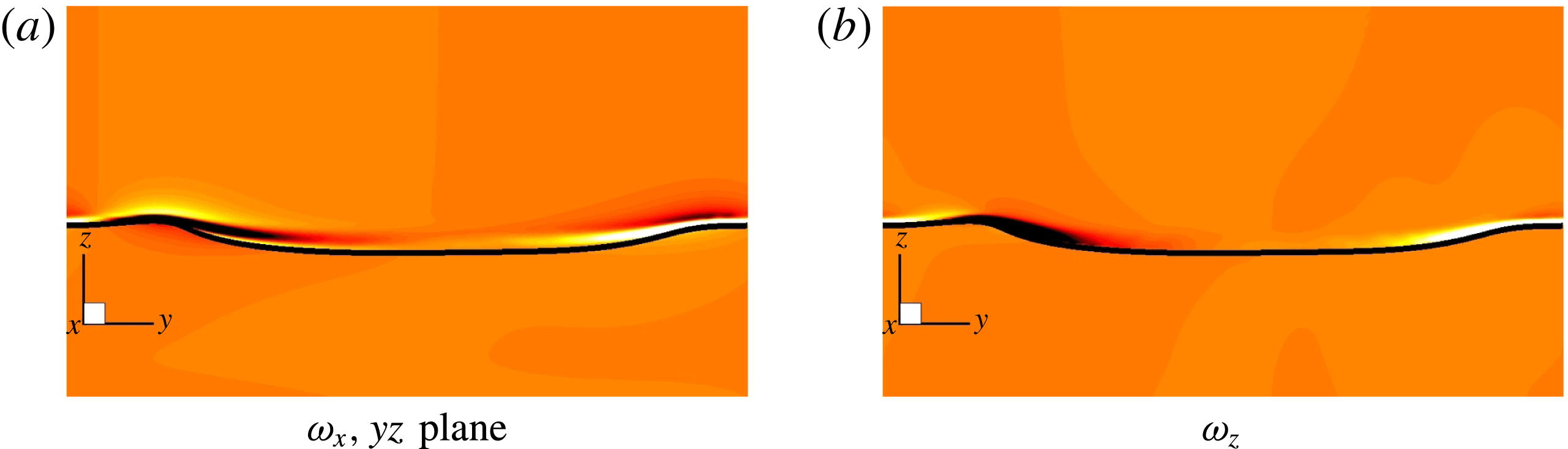
The distribution of streamwise vorticity
 $\unicode[STIX]{x1D714}_{x}$
across a wave crest in the spanwise (
 $y,z$
) plane is shown in figure 20(a) for a case wherein linear theory was found to predict well the amplification of interfacial waves in the three-dimensional simulations (see figure 15), at the point of wave overturning. The streamwise vorticity distribution is as would be expected if wave growth were governed by the flow in the (
 $x,z$
) plane: a spanwise crest moves up faster than a spanwise trough on a streamwise crest, which corresponds to negative streamwise vorticity (
 $\unicode[STIX]{x2202}w/\unicode[STIX]{x2202}y$
negative) there where the
 $y$
axis points from a spanwise wave crest to a spanwise wave trough. Furthermore, the gas flow is deflected in the spanwise direction, around a bump in the liquid, which corresponds to
 $\unicode[STIX]{x2202}v/\unicode[STIX]{x2202}z$
positive there, thus also to negative streamwise vorticity. Figure 20(a) does show this trend in this vorticity component; further above the interface,
 $\unicode[STIX]{x2202}v/\unicode[STIX]{x2202}z$
changes sign, as expected when
 $v$
tends to zero far away from the interface, and so does
 $\unicode[STIX]{x1D714}_{x}$
. Finally, inspection of the pressure field merely confirms a low-pressure region downstream of the wave crest (not shown).
To understand the corresponding distribution of the wall-normal vorticity component, we recall that in the Hinch mechanism for wave growth in the
 $(x,z)$
plane (demonstrated already to apply to two-dimensional flows), the (less viscous) gas is slowed down at wave crests through the condition of continuity of tangential stress at the interface; diffusion and advection of the corresponding spanwise vorticity cause wave growth. This will be stronger above a spanwise wave crest, thus
 $\unicode[STIX]{x2202}u/\unicode[STIX]{x2202}y$
will be positive where the
 $y$
axis points from a spanwise crest to a spanwise trough, contributing to negative
 $\unicode[STIX]{x1D714}_{z}$
there. This agrees with figure 20(b); furthermore, the linearized term in the vorticity equation that represents production of wall-normal vorticity,
 $U_{0}^{\prime }(\unicode[STIX]{x2202}w/\unicode[STIX]{x2202}y)$
, is then of the same sign.
Vorticity analysis showing streamwise and wall-normal vorticity components in a (
 $y,z$
) slice. Parameters:
 $(m=50,h_{0}=0.2,{\mathcal{G}}=0.1,We=10)$
, with
 $r=10$
and
 $Re=500$
. As before,
 $\ell _{x}=0.47$
and
 $\ell _{y}=0.97$
. The same colour range has been used in both panels.

Motivated by the above considerations, we recall the mechanism for the generation of the cross-flow velocity under the linear theory, casting this in terms of vortex stretching and reorientation, with a view to demonstrating that the same mechanism persists and is reinforced under the nonlinear dynamics. In linear theory, wall-normal vorticity is amplified for modes with
 $\unicode[STIX]{x1D6FD}\neq 0$
via vortex stretching. By Squire’s equation (for consistency with what follows, we use
 $\unicode[STIX]{x1D714}_{z}$
instead of
 $\unicode[STIX]{x1D702}$
for the wall-normal vorticity):
 $$\begin{eqnarray}\displaystyle & \displaystyle {\displaystyle \frac{\unicode[STIX]{x2202}\unicode[STIX]{x1D714}_{z}}{\unicode[STIX]{x2202}t}}+U_{0}{\displaystyle \frac{\unicode[STIX]{x2202}\unicode[STIX]{x1D714}_{z}}{\unicode[STIX]{x2202}x}}=-U_{0}^{\prime }{\displaystyle \frac{\unicode[STIX]{x2202}w}{\unicode[STIX]{x2202}y}}+{\displaystyle \frac{1}{Re}}\unicode[STIX]{x1D6FB}^{2}\unicode[STIX]{x1D714}_{z},\quad \unicode[STIX]{x1D714}_{z}=\hat{\boldsymbol{z}}\boldsymbol{\cdot }(\unicode[STIX]{x1D735}\times \boldsymbol{u}). & \displaystyle\end{eqnarray}$$
In this context,
 $-U_{0}^{\prime }$
corresponds to the base-state contribution to the spanwise vorticity
 $\unicode[STIX]{x1D714}_{y}$
. Equation (6.3) makes clear the origin of the ‘liftup mechanism’ in three-dimensional linear stability theory (Schmid & Henningson Reference Schmid and Henningson2001), as this equation is essentially the
 $z$
component of the linearized vortex-stretching equation, and it implies that vorticity is transferred from the spanwise to the wall-normal direction via the production term
 $-U_{0}^{\prime }(\unicode[STIX]{x2202}w/\unicode[STIX]{x2202}y)$
.
Further examination of the flow structure – the same case as figure 20. Isosurfaces of
 $\unicode[STIX]{x1D714}_{z}=\pm 200$
are displayed at the various times indicated. (a) A slice is shown corresponding to the velocity gradient
 $\unicode[STIX]{x2202}w/\unicode[STIX]{x2202}y$
. (e) A slice is shown corresponding to
 $\unicode[STIX]{x2202}w/\unicode[STIX]{x2202}z$
. These are to indicate the terms that dominate in the vortex-stretching equation and are responsible for the amplification of the wall-normal vorticity.

The amplification of wall-normal vorticity continues into the nonlinear regime beyond the point of wave overturning, and the wall-normal vorticity interacts with successive crests in the train in the nonlinear regime (see figure 21). The fully nonlinear analogue of (6.3) is then
 $$\begin{eqnarray}\displaystyle & \displaystyle {\displaystyle \frac{\unicode[STIX]{x2202}\unicode[STIX]{x1D714}_{z}}{\unicode[STIX]{x2202}t}}+\boldsymbol{u}\boldsymbol{\cdot }\unicode[STIX]{x1D735}\unicode[STIX]{x1D714}_{z}=\unicode[STIX]{x1D714}_{x}{\displaystyle \frac{\unicode[STIX]{x2202}w}{\unicode[STIX]{x2202}x}}+\unicode[STIX]{x1D714}_{y}{\displaystyle \frac{\unicode[STIX]{x2202}w}{\unicode[STIX]{x2202}y}}+\unicode[STIX]{x1D714}_{z}{\displaystyle \frac{\unicode[STIX]{x2202}w}{\unicode[STIX]{x2202}z}}+{\displaystyle \frac{1}{Re}}\unicode[STIX]{x1D6FB}^{2}\unicode[STIX]{x1D714}_{z}. & \displaystyle\end{eqnarray}$$
It is therefore of interest to examine which of the velocity gradient terms in (6.4) has the largest magnitude, since this will provide the largest contribution to the stretching of the wall-normal vorticity. For early times, a slice through the three-dimensional isosurface in figure 21(a) reveals that
 $\unicode[STIX]{x2202}w/\unicode[STIX]{x2202}y$
is the largest velocity-gradient term, indicating a mechanism whereby
 $\unicode[STIX]{x1D714}_{y}(\unicode[STIX]{x2202}w/\unicode[STIX]{x2202}y)$
contributes to the stretching of the wall-normal vorticity. This route is identical to the route in linear theory (equation (6.3)), which adds consistency to the above argument and suggests that the small-amplitude mechanism of vorticity amplification carries over to the nonlinear regime. The amplified vorticity is advected downstream by the mean flow, as in figure 21(b,c), to the point where it sits on top of a downstream streamwise wave crest, as in figure 21(d,e). Further secondary sheets of wall-normal vorticity are produced as time goes by. These are located close to the interface. A slice in figure 21(e) indicates that
 $(\unicode[STIX]{x2202}w/\unicode[STIX]{x2202}z)$
is the velocity gradient term of largest magnitude, thereby suggesting further wall-normal vortex stretching by the term
 $\unicode[STIX]{x1D714}_{z}(\unicode[STIX]{x2202}w/\unicode[STIX]{x2202}z)$
. This corresponds to a fully nonlinear process, absent from the linearized equation (6.3).
Further regions of intense wall-normal vorticity are created near the spanwise wave crest, are advected downstream, and are focused in the downstream region where the existing vorticity lies, leading to a complicated chaotic flow as in figure 21(e–g). In summary, the mechanism implied by (6.3) for the amplification of wall-normal vorticity holds up in the nonlinear regime, and is supplemented by the fact that vorticity zones created by downstream/upstream crests interact to create a complicated flow pattern that eventually results in a complex liquid dispersion embedded in the gas phase.
Although the conclusions drawn here are for a single case, the theoretical description contained herein is based on wave amplification in linear theory, and a reinforcement of the same by nonlinear mechanisms, and is therefore generic, and may apply to other parameter regimes also. We have seen in some cases, however, that the flow behaviour is nearly two-dimensional. We have therefore inspected also the vorticity field in the case wherein a capillary ridge is formed, of which the interface evolution is shown in figure 17 (lower row), for
 $r=100$
at
 $h=0.2,m=50,Re_{L}=30,{\mathcal{G}}_{L}=1$
and
 $We=10$
. Although the streamwise vorticity is qualitatively similar to that identified above, it is less pronounced, and it is now also shed from the spanwise wave crest, whereas the vorticity distributions on the spanwise wave sides in the above are bent around the spanwise wave crest. The fact that in this case no significant spanwise perturbation in the interface shape results, we attribute to the comparatively strong inertia of the liquid compared to that of the gas.
7 Discussion and conclusions
Summarizing, we have investigated the mechanisms that produce three-dimensional waves in otherwise two-dimensional parallel laminar gas–liquid flows, focusing on the Reynolds number and the density contrast as the key parameters. In all considered cases, the linear theory provides a reliable starting point for understanding the development of three-dimensional waves, through (eigenvalue) Orr–Sommerfeld–Squire theory; this has been established through comparison of the growth rate obtained from DNS with linear theory, as well as by inspection of the vorticity fields. Specifically, we have established that the vorticity field in two-dimensional wave growth is consistent with the mechanism proposed by Hinch (Reference Hinch1984), and that this persists to close to wave overturning (see § 5.3). The same reasoning carries over to the three-dimensional cases (§ 6.2).
For the reference cases at low density ratios, the flow is mostly unstable due to a shear mode, and a strongly two-dimensional pattern of linearly unstable interfacial waves persists until late time, although the interfacial waves eventually assume a dramatically three-dimensional character (e.g. figure 13), due to the rollup and subsequent breakup of liquid ‘sheets’ – these being a simple three-dimensional analogue of two-dimensional ligaments. For moderately large density ratios, the Yih mechanism prevails, and the three-dimensional disturbances are more prominent from the start, in some cases leading to violent flow behaviour. This is explained by the linear theory wherein intermediate density ratios lead to a larger number of unstable spanwise modes. At large density ratios, the growth rate of linear modes weakens substantially, albeit that the cutoff wavenumbers increase, such that saturated waves with well-defined three-dimensional features emerge, although a huge wave is formed in some cases at moderately large density ratio that appears not to prevail due to the associated pressure drop required to maintain it (see figure 10). These observations have been placed in a systematic framework using a flow-pattern map for two-dimensional systems, in terms of density ratio, Reynolds number and Weber number; corresponding three-dimensional simulations are demonstrated to exhibit similar behaviour.
Spectral analysis of the three-dimensional simulations indicate that the linear theory plays a very visible role in generating both two-dimensional and three-dimensional waves, of which the latter are more prominent at moderate to large density contrasts (e.g. figures 15 and 19). The late-time highly nonlinear behaviour of the interface therefore has its origin in the linear theory, across the range of density ratios. The basic mechanism for feeding energy into the interface also survives into the nonlinear regime, as evidenced by the above vorticity arguments. At low to intermediate density ratios, the resulting complicated interfacial structures have their own peculiar features that are unique to the nonlinear regime (e.g. figures 13 and 16). Overall, the picture is therefore one in which the linear regime and the eventual nonlinear regime are closely coupled. This further underscores the importance of using a linear theory based on accurate base-state modelling.
Acknowledgements
This work used the ARCHER UK National Supercomputing Service (access to the facilities of ARCHER was provided through the ARCHER Resource Allocation Panel (project number e174)), and the Ada facilities of GENCI (France) under project A0012B06893. L.ÓN also acknowledges the DJEI/DES/SFI/HEA Irish Centre for High-End Computing (ICHEC) for the provision of further computational facilities and support (project number ndmat024b); L.ÓN also gratefully acknowledges a visiting professor award at the École Centrale de Lyon and a UCD Seed Funding grant (SF 1316). The authors are very grateful to Dr Z. Solomenko of École Centrale de Lyon for assistance with the numerical simulations. P.D.M.S. is very grateful to his colleague and former supervisor A. Biesheuvel for useful and stimulating discussions and suggestions.
Appendix A. Full formulation of the linear stability analysis
Here, we give a detailed formulation of the governing equations underlying the linear stability analysis undertaken in § 4.
A.1 Base state
Under the assumption of a steady, laminar and incompressible flow in both phases, driven by a constant negative pressure drop
 $\text{d}p_{0}/\text{d}x$
, the Navier–Stokes equations governing the undisturbed base flow reduce to standard balances between pressure as well as viscous and gravitational forces. This results in a flat interface
 $\unicode[STIX]{x1D709}=0$
, a unidirectional flow (
 $v=w=0$
, and
 $u=U_{0}(z)$
), and a pressure field
 $p=(\text{d}p_{0}/\text{d}x)x$
. The analytic solution for the laminar velocity profile is then
 $$\begin{eqnarray}\displaystyle & \displaystyle U_{0}(z)=\left\{\begin{array}{@{}ll@{}}U_{L}(z)=-{\displaystyle \frac{Re}{2m}}z^{2}+Az,\quad & 0\leqslant z\leqslant h_{0},\\[12.0pt] U_{G}(z)=-{\displaystyle \frac{Re}{2}}(z-1)^{2}+B(z-1),\quad & h_{0}\leqslant z\leqslant 1.\end{array}\right. & \displaystyle\end{eqnarray}$$
The constants
 $A$
and
 $B$
are determined from continuity of velocity and shear stress at the interface:
 $$\begin{eqnarray}\displaystyle & \displaystyle U_{L}(h_{0})=U_{G}(h_{0}),\quad mU_{L}^{\prime }(h_{0})=U_{G}^{\prime }(h_{0}), & \displaystyle\end{eqnarray}$$
which yields
 $$\begin{eqnarray}\displaystyle & \displaystyle {\displaystyle \frac{A}{Re}}={\displaystyle \frac{{\textstyle \frac{1}{2}}(h_{0}-1)(h_{0}+1)-h_{0}^{2}/(2m)}{h_{0}-m(h_{0}-1)}},\quad B=mA+Re. & \displaystyle\end{eqnarray}$$
A.2 Small-amplitude perturbations
In § 4 we study the stability of the base state (A 1) with respect to a small-amplitude three-dimensional perturbation. Each flow variable is expressed as a sum of the base state and the perturbation:
 $$\begin{eqnarray}\displaystyle \left.\begin{array}{@{}ll@{}}\displaystyle \unicode[STIX]{x1D709}=h_{0}+\unicode[STIX]{x1D716}\unicode[STIX]{x1D709}_{0}\text{e}^{\text{i}(\unicode[STIX]{x1D6FC}x+\unicode[STIX]{x1D6FD}y-\unicode[STIX]{x1D714}t)},\quad & w=\unicode[STIX]{x1D716}\widetilde{w}(z)\text{e}^{\text{i}(\unicode[STIX]{x1D6FC}x+\unicode[STIX]{x1D6FD}y-\unicode[STIX]{x1D714}t)},\\[3.0pt] \displaystyle \unicode[STIX]{x1D702}=\unicode[STIX]{x1D716}\widetilde{\unicode[STIX]{x1D702}}(z)\text{e}^{\text{i}(\unicode[STIX]{x1D6FC}x+\unicode[STIX]{x1D6FD}y-\unicode[STIX]{x1D714}t)},\quad & p=(\text{d}p_{0}/\text{d}x)x+\unicode[STIX]{x1D716}\widetilde{p}(z)\text{e}^{\text{i}(\unicode[STIX]{x1D6FC}x+\unicode[STIX]{x1D6FD}y-\unicode[STIX]{x1D714}t)}.\end{array}\right\} & & \displaystyle\end{eqnarray}$$
Here
 $\unicode[STIX]{x1D716}$
is the infinitesimally small amplitude of the wave and
 $\unicode[STIX]{x1D709}_{0}$
is its phase (with
 $|\unicode[STIX]{x1D709}_{0}|=1$
), and
 $\unicode[STIX]{x1D714}=c\unicode[STIX]{x1D6FC}$
, where
 $\unicode[STIX]{x1D714}$
is the complex frequency and
 $c$
the complex phase speed. Substituting equations (A 4) into the linearized Navier–Stokes equations (linearized around the base state (A 1)), we get the following system of governing equations:
 $$\begin{eqnarray}\displaystyle & \displaystyle \text{i}\unicode[STIX]{x1D6FC}rRe[(\widetilde{w}_{L}^{\prime \prime }-k^{2}\widetilde{w}_{L})(U_{L}-c)-\widetilde{w}_{B}U_{L}^{\prime \prime }]=m(\widetilde{w}_{L}^{\prime \prime \prime \prime }-2k^{2}\widetilde{w}_{L}^{\prime \prime }+k^{4}\widetilde{w}_{L}), & \displaystyle\end{eqnarray}$$
 $$\begin{eqnarray}\displaystyle & \displaystyle \text{i}rRe[\unicode[STIX]{x1D6FC}\widetilde{\unicode[STIX]{x1D702}}_{L}(U_{L}-c)+\unicode[STIX]{x1D6FD}U_{L}^{\prime }\widetilde{w}_{L}]=m(\widetilde{\unicode[STIX]{x1D702}}_{L}^{\prime \prime }-k^{2}\widetilde{\unicode[STIX]{x1D702}}_{L}), & \displaystyle\end{eqnarray}$$
in the liquid (bottom) phase, with
 $k^{2}=\unicode[STIX]{x1D6FC}^{2}+\unicode[STIX]{x1D6FD}^{2}$
, and
 $$\begin{eqnarray}\displaystyle & \displaystyle \text{i}\unicode[STIX]{x1D6FC}Re[(\widetilde{w}_{G}^{\prime \prime }-k^{2}\widetilde{w}_{G})(U_{G}-c)-\widetilde{w}_{G}U_{G}^{\prime \prime }]=\widetilde{w}_{G}^{\prime \prime \prime \prime }-2k^{2}\widetilde{w}_{G}^{\prime \prime }+k^{4}\widetilde{w}_{G}, & \displaystyle\end{eqnarray}$$
 $$\begin{eqnarray}\displaystyle & \displaystyle \text{i}Re[\unicode[STIX]{x1D6FC}\widetilde{\unicode[STIX]{x1D702}}_{G}(U_{G}-c)+\unicode[STIX]{x1D6FD}U_{G}^{\prime }\widetilde{w}_{T}]=\widetilde{\unicode[STIX]{x1D702}}_{G}^{\prime \prime }-k^{2}\widetilde{\unicode[STIX]{x1D702}}_{G}, & \displaystyle\end{eqnarray}$$
in the gas (top) phase. These are supplemented with the following no-slip and no-penetration boundary conditions:
 $$\begin{eqnarray}\displaystyle & \displaystyle \widetilde{w}=\widetilde{w}^{\prime }=\widetilde{\unicode[STIX]{x1D702}}=0 & \displaystyle\end{eqnarray}$$
at the walls
 $z=0$
and
 $z=1$
. In addition, matching conditions are prescribed at the interface
 $z=\unicode[STIX]{x1D709}_{0}$
. In the streamwise direction, continuity of velocity and tangential stress and the jump condition in the normal stress imply the following relations:
 $$\begin{eqnarray}\displaystyle & \displaystyle \widetilde{w}_{L}=\widetilde{w}_{G}, & \displaystyle\end{eqnarray}$$
 $$\begin{eqnarray}\displaystyle & \displaystyle \widetilde{w}_{L}^{\prime }+\unicode[STIX]{x1D709}_{0}U_{L}^{\prime }=\widetilde{w}_{G}^{\prime }+\unicode[STIX]{x1D709}_{0}U_{G}^{\prime },\quad \unicode[STIX]{x1D709}_{0}=\widetilde{w}_{L}/(c-U_{L})=\widetilde{w}_{G}/(c-U_{G}), & \displaystyle\end{eqnarray}$$
 $$\begin{eqnarray}\displaystyle & \displaystyle m(\widetilde{w}_{L}^{\prime \prime }+k^{2}\widetilde{w}_{L})=\widetilde{w}_{G}^{\prime \prime }+k^{2}\widetilde{w}_{G}, & \displaystyle\end{eqnarray}$$
 $$\begin{eqnarray}\displaystyle & & \displaystyle \displaystyle \text{i}\unicode[STIX]{x1D6FC}rRe[\widetilde{w}_{L}(c-U_{L})+\widetilde{w}_{L}U_{L}^{\prime }]+m(\widetilde{w}_{L}^{\prime \prime \prime }-3k^{2}\widetilde{w}_{L})\nonumber\\ \displaystyle & & \displaystyle \quad \displaystyle =\text{i}\unicode[STIX]{x1D6FC}Re[\widetilde{w}_{G}^{\prime }(c-U_{G})+\widetilde{w}_{G}U_{G}^{\prime }]+(\widetilde{w}_{G}^{\prime \prime \prime }-3k^{2}\widetilde{w}_{G})\nonumber\\ \displaystyle & & \displaystyle \quad \displaystyle +\,k^{2}\left({\mathcal{G}}+{\displaystyle \frac{k^{2}}{We}}\right)\left[{\displaystyle \frac{\widetilde{w}_{G}^{\prime }-\widetilde{w}_{L}^{\prime }}{\text{i}\unicode[STIX]{x1D6FC}(U_{L}^{\prime }-U_{G}^{\prime })}}\right]=0.\end{eqnarray}$$
Finally, the same physical matching conditions applied to the spanwise direction give rise to the following relations:
 $$\begin{eqnarray}\displaystyle & \displaystyle \widetilde{\unicode[STIX]{x1D702}}_{L}+\text{i}\unicode[STIX]{x1D6FD}U_{L}^{\prime }\unicode[STIX]{x1D709}_{0}=\widetilde{\unicode[STIX]{x1D702}}_{G}+\text{i}\unicode[STIX]{x1D6FD}U_{G}^{\prime }\unicode[STIX]{x1D709}_{0}, & \displaystyle\end{eqnarray}$$
 $$\begin{eqnarray}\displaystyle & \displaystyle m\widetilde{\unicode[STIX]{x1D702}}_{L}^{\prime }=\widetilde{\unicode[STIX]{x1D702}}_{G}. & \displaystyle\end{eqnarray}$$
Equations (A 5)–(A 7) constitute an eigenvalue problem for the velocities
 $(\widetilde{w}_{L},\widetilde{w}_{G})$
and vorticity components
 $(\widetilde{\unicode[STIX]{x1D702}}_{L},\widetilde{\unicode[STIX]{x1D702}}_{G})$
, with eigenvalue
 $\unicode[STIX]{x1D706}=-\text{i}\unicode[STIX]{x1D6FC}c=-\text{i}\unicode[STIX]{x1D714}$
. They can be formulated in the operator/matrix form given in (3.1), of which the latter can be solved numerically using the standard Chebyshev collocation techniques (Boomkamp et al.
Reference Boomkamp, Boersma, Miesen and Beijnon1997).
A.3 Energy-budget analysis
To understand the physical mechanism that causes the instability, we perform an energy-budget analysis, focusing on two-dimensional disturbances for which
 $v=0$
. We multiply the corresponding linearized equations of motion for the perturbation velocity
 $\unicode[STIX]{x1D6FF}\boldsymbol{u}=(\unicode[STIX]{x1D6FF}u,0,\unicode[STIX]{x1D6FF}w)$
by
 $\unicode[STIX]{x1D6FF}\boldsymbol{u}$
itself and integrate over the
 $x$
and
 $z$
directions (the corresponding perturbation pressure is denoted by
 $\unicode[STIX]{x1D6FF}p$
). The
 $x$
variable is integrated over a single wavelength
 $\ell _{0}=2\unicode[STIX]{x03C0}/\unicode[STIX]{x1D6FC}$
and the
 $z$
variable is integrated over the full vertical extent of the channel. In a standard fashion, this gives the following energy-budget relation:
 $$\begin{eqnarray}\displaystyle & \displaystyle \mathop{\sum }_{j=L,G}KIN_{j}=\mathop{\sum }_{j=L,G}REY_{j}+\mathop{\sum }_{j=L,G}DISS_{j}+INT, & \displaystyle\end{eqnarray}$$
where
 $$\begin{eqnarray}\displaystyle & \displaystyle KIN_{j}={\displaystyle \frac{1}{2}}{\displaystyle \frac{\text{d}}{\text{d}t}}\int \text{d}x\int \text{d}z\,r_{j}\unicode[STIX]{x1D6FF}\boldsymbol{u}_{j}^{2}, & \displaystyle\end{eqnarray}$$
 $$\begin{eqnarray}\displaystyle & \displaystyle REY_{j}=-r_{j}\int \text{d}x\int \text{d}z\,\unicode[STIX]{x1D6FF}u_{j}\unicode[STIX]{x1D6FF}w_{j}{\displaystyle \frac{\text{d}U_{0}}{\text{d}z}}, & \displaystyle\end{eqnarray}$$
 $$\begin{eqnarray}\displaystyle & \displaystyle DISS_{j}=-{\displaystyle \frac{m_{j}}{Re}}\int \text{d}x\int \text{d}z\,\left[2\left({\displaystyle \frac{\unicode[STIX]{x2202}}{\unicode[STIX]{x2202}x}}\unicode[STIX]{x1D6FF}u_{j}\right)^{2}+2\left({\displaystyle \frac{\unicode[STIX]{x2202}}{\unicode[STIX]{x2202}z}}\unicode[STIX]{x1D6FF}w_{j}\right)^{2}+\left({\displaystyle \frac{\unicode[STIX]{x2202}}{\unicode[STIX]{x2202}z}}\unicode[STIX]{x1D6FF}u_{j}+{\displaystyle \frac{\unicode[STIX]{x2202}}{\unicode[STIX]{x2202}x}}\unicode[STIX]{x1D6FF}w_{j}\right)^{2}\right]. & \displaystyle \nonumber\\ \displaystyle & & \displaystyle\end{eqnarray}$$
Here,
 $j=L,G$
, with
 $r_{G}=1$
and
 $r_{L}=r$
, and similarly for
 $m_{j}$
. The term ‘
 $INT$
’ is related to interfacial conditions, and is given in terms of the following stress tensor for the perturbed flow, where
 $$\begin{eqnarray}\displaystyle & \displaystyle \unicode[STIX]{x1D61B}_{xx,j}=-\unicode[STIX]{x1D6FF}p+{\displaystyle \frac{2m_{j}}{Re}}{\displaystyle \frac{\unicode[STIX]{x2202}}{\unicode[STIX]{x2202}x}}\unicode[STIX]{x1D6FF}u,\quad \unicode[STIX]{x1D61B}_{zz,j}=-\unicode[STIX]{x1D6FF}p+{\displaystyle \frac{2m_{j}}{Re}}{\displaystyle \frac{\unicode[STIX]{x2202}}{\unicode[STIX]{x2202}z}}\unicode[STIX]{x1D6FF}w,\quad \unicode[STIX]{x1D61B}_{xz,j}={\displaystyle \frac{m_{j}}{Re}}\left({\displaystyle \frac{\unicode[STIX]{x2202}}{\unicode[STIX]{x2202}z}}\unicode[STIX]{x1D6FF}u+{\displaystyle \frac{\unicode[STIX]{x2202}}{\unicode[STIX]{x2202}x}}\unicode[STIX]{x1D6FF}w\right). & \displaystyle \nonumber\\ \displaystyle & & \displaystyle\end{eqnarray}$$
Thus,
 $$\begin{eqnarray}\displaystyle & \displaystyle INT=\int _{0}^{\ell _{0}}\text{d}x\,[\unicode[STIX]{x1D6FF}u_{L}\unicode[STIX]{x1D61B}_{xz,L}+\unicode[STIX]{x1D6FF}w_{L}\unicode[STIX]{x1D61B}_{zz,L}]_{z=0}-\int _{0}^{\ell _{0}}\text{d}x\,[\unicode[STIX]{x1D6FF}u_{G}\unicode[STIX]{x1D61B}_{xz,G}+\unicode[STIX]{x1D6FF}w_{G}\unicode[STIX]{x1D61B}_{zz,G}]_{z=0}, & \displaystyle\end{eqnarray}$$
which is decomposed into normal and tangential contributions,
 $$\begin{eqnarray}\displaystyle & \displaystyle INT=NOR+TAN, & \displaystyle\end{eqnarray}$$
where
 $$\begin{eqnarray}\displaystyle & \displaystyle NOR=\int _{0}^{\ell _{0}}\text{d}x\,[\unicode[STIX]{x1D6FF}w_{L}\unicode[STIX]{x1D61B}_{zz,L}-\unicode[STIX]{x1D6FF}w_{G}\unicode[STIX]{x1D61B}_{zz,G}]_{z=0} & \displaystyle\end{eqnarray}$$
and
 $$\begin{eqnarray}\displaystyle & \displaystyle TAN=\int _{0}^{\ell _{0}}\text{d}x\,[\unicode[STIX]{x1D6FF}u_{L}\unicode[STIX]{x1D61B}_{xz,L}-\unicode[STIX]{x1D6FF}u_{G}\unicode[STIX]{x1D61B}_{xz,G}]_{z=0}. & \displaystyle\end{eqnarray}$$
Appendix B. A sample grid-refinement study
The numerical method has been tested extensively in Solomenko et al. (Reference Solomenko, Spelt, Ó Náraigh and Alix2017) on basic tests and various two-phase flows. It is a further improvement of the method used and tested in Ó Náraigh et al. (Reference Ó Náraigh, Valluri, Scott, Bethune and Spelt2014) for the present problem in the special case of density-matched fluids. We complement these tests here with a sample grid-refinement study for the parameter case
 $(m=30,h_{0}=0.3,{\mathcal{G}}=1,We=100,Re=100)$
, and with
 $r=5$
, based on upper-layer scaling. We focus on two-dimensional simulations, wherein the number of grid points in the
 $x$
and
 $z$
directions is denoted by
 $N_{x}$
and
 $N_{z}$
, respectively. We present results for three simulations, with
 $(N_{x},N_{z})=(289,201),~(353,245)$
and
 $(481,335)$
, with time step
 $\unicode[STIX]{x0394}t=10^{-4},~5\times 10^{-5}$
and
 $2\times 10^{-5}$
, respectively, designed to keep the CFL number
 $\max (U_{L},U_{G})\unicode[STIX]{x0394}t(N_{z}-1)$
approximately constant. All of the simulations in this appendix are initialized with a monochromatic disturbance at the interface,
 $\unicode[STIX]{x1D709}(x,t=0)=h_{0}+0.001\cos [(2\unicode[STIX]{x03C0}/L_{x})x]$
; the initial velocity and pressure are taken to be those of the base state.
The
 $L^{2}$
norm of the
 $w$
velocity for the three simulations in the sample grid-refinement study. The parameter values for the study are based on upper-layer scaling and are given as
 $(m=30,h_{0}=0.3,{\mathcal{G}}=1,We=100,Re=100)$
; also,
 $r=5$
.

Detailed quantitative comparison between numerics and Orr–Sommerfeld theory for the low-resolution case
 $(N_{x},N_{z})=(289,201)$
. (a) There is agreement between the numerically computed growth rate and the theoretical one derived from Orr–Sommerfeld analysis. (b) The same agreement for the wave period: the time evolution of the wall-normal velocity
 $w(x=L_{x}/2,z=L_{z}/2,t)$
in the DNS. The time
 $T_{DNS}$
between successive maxima in
 $w(x=L_{x}/2,z=L_{z}/2,t)$
is computed. This is compared with the wave period
 $T_{OS}$
from the Orr–Sommerfeld theory. The error in
 $T_{DNS}$
is due to the sampling rate associated with the periodic output of data to files. (c) The agreement between the flow structure in the numerics and the theory – shown is the wall-normal velocity at the crest of the wave, normalized by the height of the wave. This facilitates a precise comparison between the numerics and the theory.

Grid-refinement study in the nonlinear regime: shown is the ligament structure at
 $t=4$
for the two higher-resolution numerical simulations. The parameter values (based on upper-layer scaling) in (a) are as before:
 $(m=30,h_{0}=0.3,{\mathcal{G}}=1,We=100,Re=100)$
, also,
 $r=5$
; in (b),
 $We=10$
.

We compare and contrast the simulations. Our starting point is the linear regime. As such, figure 22 shows a plot of the
 $L^{2}$
norm of the
 $w$
velocity as a function of time, i.e.
 $\Vert w\Vert _{2}^{2}(t)=\int _{0}^{\ell _{x}}\!\int _{0}^{1}[w(x,z,t)]^{2}\,\text{d}x\,\text{d}z$
, which is appropriate for studying the linear regime, as
 $\Vert w\Vert _{2}^{2}(t)$
will grow exponentially when the system is in an unstable Orr–Sommerfeld mode. Figure 22 demonstrates that the numerical simulations behave identically in the linear regime at all resolutions. Accordingly, we demonstrate the agreement between linear theory and the numerical simulations for the lowest-resolution case in figure 23, where the system behaviour is in line with modal Orr–Sommerfeld theory.
We further focus on the nonlinear regime in figure 24(a), where we look at the formation of ligaments at the later time
 $t=4.0$
in the two higher-resolution cases. There is very close agreement between the two simulations, indicating that the results are close to having fully converged. At least some of the (small) differences between the two simulations can be attributed to the slightly different domain sizes in each case, with
 $L_{x}=353/245$
and
 $L_{x}=481/335$
in the two different simulations. Such small differences are unavoidable in the parallel simulations, as
 $N_{x}-1$
must be chosen to be a multiple of the number of compute cores used (32 in all simulations in this appendix). Furthermore, we emphasize that the results are qualitatively very similar in the two cases, meaning that the qualitative conclusions drawn in the main part of the paper regarding flow regimes and interfacial structures are robust. The conclusions are furthermore robust to changes in the Weber number, as evidenced by a further grid sensitivity study at
 $We=10$
shown in figure 24(b).