


1. Introduction
In the statistical literature, there is little debate as to whether testing statistical hypotheses is the most controversial aspect of statistical inference, with at least three major competing schools approaching the problem from different angles and often concluding with opposite decisions. In this regard, Lindley’s (Reference Lindley1957) paradox may constitute the most quoted instance of the opposition between the frequentist and the Bayesian schools of inference. Two recent reassessments of the paradox appeared in Philosophy of Science, with Spanos (Reference Spanos2013) and Sprenger (Reference Sprenger2013) diverging in their resolution of the paradox, which prompted me to reconsider in turn this fundamental argument both in the frequentist-Bayesian debate and in the derivation of (more) coherent testing procedures within the Bayesian framework.
Let me first recall the setting of the paradox as exposed in Lindley (Reference Lindley1957), often called the Jeffreys-Lindley paradox after Dennis Lindley pointed out the facts that were already exposed in Jeffreys (Reference Jeffreys1939). Given a sample of size n from a normal distribution 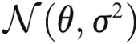 with known variance
 , testing whether the null hypothesis
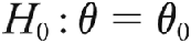 on the mean holds (against the alternative
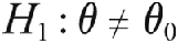 ) may lead to opposite conclusions depending on the statistical perspective adopted to conduct the test. Namely, summarizing the data set into the sufficient statistic
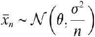
leads to the t-statistic  , which is distributed as an
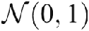 variable under the null hypothesis, allowing for the computation of the p-value equal to

where  is a generic notation for a probability computation and p(·) is the symbol used here for the p-value function. Relying on this p-value to determine (or decide) whether H 0 holds means examining its numerical value either in absolute terms (as suggested by Fisher) or with respect to a bound (as suggested by Neyman and Pearson). A Bayesian approach to the hypothesis-testing problem, as exposed in Jeffreys (Reference Jeffreys1939), relies on the ratio of evidences (or marginal likelihoods) also called the Bayes factor (see Berger Reference Berger1985; Robert Reference Robert2001). When the prior distribution on the parameter
 happens to be the normal prior,
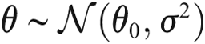 , the Bayes factor is given by

which measures the evidence brought by the data in favor of the null hypothesis relative to the alternative hypothesis. A decision about which hypothesis to select is then based on the numerical value of 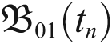 , the default boundary between the null and the alternative being
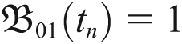 since the data then bring the same evidence in favor of both hypotheses.
The paradox exposed by Lindley (Reference Lindley1957) is that, for a fixed numerical value of tn and for almost any choice of prior distribution on  , the Bayes factor
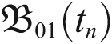 goes to infinity with the sample size n, while the p-value p(tn) remains constant in n. In Lindley’s words, “we [can be] 95% confident [as frequentists] that
 but have 95% belief [as Bayesians] that
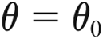 ” (187). This occurs, for instance, when tn = 1.96 and n = 16,818, assuming the prior weights equally both hypotheses. (And for n = 164 if H 0 is 10 times more likely than H 1.) Sprenger (Reference Sprenger2013) takes the example of a test for extrasensory capacities to oppose a p-value of .003 and a Bayes factor of 12 in favor of the null. This divergence of outcomes is called a “paradox” since the same data set almost certainly leads to opposite conclusions and hence decisions when the sample size n is large. It led many commentators of the paradox to conclude that one approach or the other was “wrong.”
While divergences between different statistical theories of inference and their numerical conclusions are to be expected, the surprising phenomenon that they persist when the sample size grows to infinity explains the long-term impact of this paradox and the fact that it is still the focus of attention for statisticians and philosophers of science alike. Although the frequentist-Bayesian opposition expressed by the paradox can be thoroughly explained, the Jeffreys-Lindley paradox also has foundational consequences within the Bayesian framework that are detailed in section 2.1.
Indeed, my personal apprehension of the Jeffreys-Lindley paradox is that it points at the poor (and even unacceptable) behavior of improper prior distributions when testing point-null hypotheses. An illustration is the resolution proposed in Robert (Reference Robert1993) aimed at suppressing the impact of an arbitrary normalizing constant in improper priors. This perspective is exposed in section 2.2, while some possible Bayesian resolutions are indicated in section 4, without engaging the reader into a technical foray that would not bring further insight on the concepts at work behind the Jeffreys-Lindley paradox. However, a large majority of quotes and comments found in the literature view the paradox as an irreconcilable divergence between the Bayesian and the frequentist resolutions of the point-null hypothesis-testing problem, blaming (at least) one of those approaches for the discrepancy. This point of view is debated and criticized in section 2.1 and to a larger extent in section 3. As the article starts with an analysis of the opposition between the p-value and the Bayes factor (see, e.g., Kass and Wasserman Reference Kass and Wasserman1996), I want to stress that my Bayesian approach follows the decision-theoretic perspective advocated by Berger (Reference Berger1985), which means that hypothesis testing is conducted with the intent of a course of action (depending on the selection or rejection of H 0) rather than for the epistemic attempt of uncovering the “truth,” agreeing in this respect with the position advocated in Sprenger (Reference Sprenger2013).Footnote 1
The plan of this article is as follows: it reviews the different perspectives on the paradox in section 2, it analyses and rebuts the recent criticism of Spanos (Reference Spanos2013) in section 3, it studies some Bayesian resolutions of the paradox in section 4, and it concludes in section 5.
2. Setting the Paradox Referentials
2.1. Frequentist versus Bayesian Interpretations
Let us recall that the classical view of the Jeffreys-Lindley paradox is that the Bayes factor and the p-value asymptotically (in the sample size) differ to the point of leading to opposite conclusions (acceptance vs. rejection of the null hypothesis H 0). There is obviously no mathematical issue with the paradox—otherwise it would have been readily dismissed—as the quantities involved in the two perspectives evaluate different objects using different measures: the probability measure of an event over the sample space versus the probability measure of an event over the parameter space, the former being conditional on the parameter value and the later on the observation of the sample. Despite the large literature on the topic, I would also argue that this is not a statistical paradox on the basis of the argument that observing a constant value of tn as n increases is not of statistical interest:Footnote 2 when H 0 is true, tn has a limiting 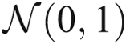 distribution, which means the corresponding p-value has a limiting uniform distribution, while, when H 0 does not hold, tn converges almost surely to ∞, in which case both the Bayes factor and the p-value converge to 0. This behavior is completely in line with the general result of the consistency of the Bayes factor in this setting, which is all too often overlooked in most commentaries on the Jeffreys-Lindley paradox. And the Neyman-Pearson (frequentist) approach to testing suggests decreasing both the type I and type II errors, hence also decreasing the acceptance boundary for the p-value when n increases (see, e.g., Lehmann and Casella Reference Lehmann and Casella1998).
There are arguably several reasons why the two approaches, Bayesian ( ) and frequentist (
 ), should not numerically agree, even asymptotically. Those reasons all revolve around the central feature that the Bayesian perspective is the only one that allows probabilistic conditioning on the observed value x obs and solely on that value:
a) one approach (
 ) operates on the parameter space , the range of the possible values of under the alternative, while the other () is produced exclusively on the sample space under the null. They are thus covering incompatible events. The same opposition occurs between confidence () and credibility () when constructing interval estimators (a point also made by Sprenger [Reference Sprenger2013]);
b) one (
) relies solely on the point-null hypothesis H 0 and on the sampling distribution it induces, making an evaluation like the p-value absolute, while the other () opposes the null H 0 and its model to a marginal version of the models corresponding to H 1 (in the sense that those models are integrated over the parameter space against a specific prior distribution), which implies that the Bayes factor and the posterior probability of H 0 are relative;c) according to what may be the most famous quote from Jeffreys (Reference Jeffreys1939, sec. 7.2), one (
) could reject “a hypothesis that may be true … because it has not predicted observable results that have not occurred” (which means considering the event [X > x obs], say, as the new focus of inference, rather than the sole observation x obs), in contrast with the other (), which manages to condition on the observed value x obs. This implies, in particular, that the former () cannot agree with the likelihood principle (Birnbaum Reference Birnbaum1962), while the other is almost uniformly in agreement with it (Berger and Wolpert Reference Berger and Wolpert1988);Footnote 3d) at least in the Fisherian version of the frequentist perspective, one (
) resorts to an arbitrarily fixed bound on the p-value, while the other () mostly refers to a threshold set by the experimenter, rather than the default boundary probability of 1/2. In the later case, unless a genuine loss function on the consequences of a wrong decision or an unbalanced prior weighting vector is constructed, both hypotheses are weighted equally, and the boundary signifies that the data favor one hypothesis versus the other in terms of marginal likelihood values. This default principle is equivalent to using the reference 0–1 loss (Berger Reference Berger1985) and to adopting the value 1 as the pivotal value for the Bayes factor.
 ) operates on the parameter space
 , the range of the possible values of
 under the alternative, while the other (
 ) is produced exclusively on the sample space
 under the null. They are thus covering incompatible events. The same opposition occurs between confidence (
 ) and credibility (
 ) when constructing interval estimators (a point also made by Sprenger [
 ) relies solely on the point-null hypothesis H 0 and on the sampling distribution it induces, making an evaluation like the p-value absolute, while the other (
 ) opposes the null H 0 and its model to a marginal version of the models corresponding to H 1 (in the sense that those models are integrated over the parameter space
 against a specific prior distribution), which implies that the Bayes factor and the posterior probability of H 0 are relative;
 ) could reject “a hypothesis that may be true … because it has not predicted observable results that have not occurred” (which means considering the event [X > x obs], say, as the new focus of inference, rather than the sole observation x obs), in contrast with the other (
 ), which manages to condition on the observed value x obs. This implies, in particular, that the former (
 ) cannot agree with the likelihood principle (Birnbaum
 ) resorts to an arbitrarily fixed bound
 on the p-value, while the other (
 ) mostly refers to a threshold set by the experimenter, rather than the default boundary probability of 1/2. In the later case, unless a genuine loss function on the consequences of a wrong decision or an unbalanced prior weighting vector is constructed, both hypotheses are weighted equally, and the boundary signifies that the data favor one hypothesis versus the other in terms of marginal likelihood values. This default principle is equivalent to using the reference 0–1 loss (Berger
A consequent literature (see, e.g., Berger and Sellke Reference Berger and Sellke1987) has since then shown how divergent those two approaches could prove to be (to the point of being asymptotically incompatible). Despite the fact that both approaches are consistent in the sense mentioned above, most commentators on the paradox conclude by blaming the p-value (always rejecting at a given  level for n large enough) or the Bayes factor (always accepting for a fixed p-value for n large enough) or both (see, e.g., Spanos Reference Spanos2013; Sprenger Reference Sprenger2013). Others (see, e.g., Gelman et al. Reference Gelman, Carlin, Stern, Dunson, Vehtari and Rubin2013) have chosen to bypass the opposition by considering tools at the interface between both approaches, like posterior predictive checks.
2.2. Improper Inputs for Bayes Factors
While the gap between the frequentist and the Bayesian degrees of evidence was the reason for Lindley (Reference Lindley1957) mentioning a statistical paradox, an orthogonal consequence of Jeffreys’s (Reference Jeffreys1939) and Lindley’s (Reference Lindley1957) exhibiting this paradox is to highlight the genuine difficulty in using improper priors in testing settings:Footnote 4 as stressed by Lindley, “the only assumption that will be questioned is the assignment of a prior distribution of any type” (188). This was also the argument made by both Shafer (Reference Shafer1982) and DeGroot (Reference DeGroot1982; see also DeGroot Reference DeGroot1973) in their discussion of the paradox. Note that, as discussed in Robert, Chopin, and Rousseau’s (Reference Robert, Chopin and Rousseau2009, sec. 6.4) reassessment of his book, Jeffreys (Reference Jeffreys1939) does not address the general problem of using improper priors in testing, namely, that the Bayes factor may be undefined due to the lack of normalizing constants in such priors (Berger Reference Berger1985; Robert Reference Robert2001). Instead, he relies on ad hoc if effective solutions when available and more generally sketches a second (and underappreciated) type of (proper) Jeffreys’s priors for testing statistical hypotheses.
This second (but not secondary) level of interpretation for the paradox shifts the asymptotes from the sample size to a prior scale factor. If we remain within the normal framework of Lindley (Reference Lindley1957), with one observation 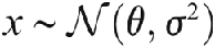 , considering a prior distribution of the form
 under the alternative hypothesis leads to a Bayes factor that is identical to equation (1) for tn = x. In this perspective, n is a prior scale factor, so that the prior variance is n times larger than the observation variance.Footnote 5 The interpretation of the phenomenon is then obviously different: when the prior scale n goes to infinity, the Bayes factor goes to infinity no matter what the value of the observation x is. (Note that both interpretations are mathematically equivalent.) Under this new light, n becomes what Lindley calls “a measure of lack of conviction about the null hypothesis” (189), a sentence that I reinterpret as the prior (under H 1) getting more and more diffuse as n grows. However, I want to stress once again that nowhere in Lindley’s article (nor in Jeffreys’s book) is the difficulty with improper priors spelled out clearly.
In this (re)interpretation of the Jeffreys-Lindley paradox, I consider that the phenomenon exhibited therein is not paradoxical in the least: when the diffuseness of the (alternative) prior (i.e., under H 1) increases, the only relevant piece of information becomes that  could be equal to
 , to the extent that it overwhelms any evidence to the contrary contained in the data. For one thing, and as put by Lindley (Reference Lindley1957, 189), “the value
 is fundamentally different from any value of
 , however near
 it might be.”Footnote 6 In addition, letting n grow to infinity means that the mass of the prior distribution in any fixed neighborhood of the null hypothesis and even in any set coherent with the data at hand vanishes to zero. There is therefore a deep coherence in the selection of the null hypothesis H 0 in this case: being completely indecisive about the alternative hypothesis means we could and should not choose this alternative. It is not possible to pick the alternative hypothesis of an undefined value of
 when opposed to the very special value
 if we want to be “completely non-informative” about
 under H 1. This analysis of the Jeffreys-Lindley paradox is justifying (further) the prohibition of the use of improper priors for testing point-null hypotheses and selecting embedded models (found, e.g., in DeGroot Reference DeGroot1982; Berger Reference Berger1985; Robert Reference Robert2001).
Depending on one’s perspective about the position of Bayesian statistics within statistical theories of inference, one might see this as a strength or as a weakness since Bayes factors and posterior probabilities do require a realistic model under the alternative when p-values and Bayesian predictives do not. A logical reason for this requirement is that Bayesian inference need proceed with the alternative model when the null is rejected. This Bayesian insight on the paradox therefore leads to the requirement to handle testing statistical hypotheses under limited prior information and within the paradigm. Solutions addressing this issue are discussed in section 4. Before this, I provide and rebut the arguments given in Spanos (Reference Spanos2013) that the Jeffreys-Lindley paradox actually highlights the deficiencies of the Bayesian approach to testing.
3. Do Not Be Afraid
Under the rather provocative title “Who Should Be Afraid of the Jeffreys-Lindley Paradox,”Footnote 7 Spanos (Reference Spanos2013) offers his frequentist reassessment of the paradox, arguing against both Bayesian and likelihood ratio approaches and in favor of the postdata severity evaluation he and Mayo have both been advocating since 2004. Answering those criticisms was the starting motivation for writing the current article.
While I hope the reader is already familiar with the contents of Spanos (Reference Spanos2013), let me first recapitulate the main points made in this article before embarking onto a more detailed analysis of those arguments. Spanos compares the frequentist (use of p-values), Bayesian (use of Bayes factors) and “likelihoodist” (use of likelihood ratios) approaches to statistical testing, with the conclusion that the latter two “give rise to highly fallacious results” (75), while the p-value can be processed (or rescued) by the postdata severity analysis of Mayo and Spanos (Reference Mayo and Spanos2004; defined below in sec. 3.3), escaping the Jeffreys-Lindley paradox. The article insists on the ability of this method to exhibit a certain degree  of discrepancy from the null hypothesis, while Bayesian and likelihoodist methods cannot and do not provide evidence for a particular alternative hypothesis (see, e.g., Spanos Reference Spanos2013, 79). Spanos concludes that the paradox “has played an important role in undermining the credibility of frequentist inference” as being “vulnerable to the fallacy of rejection” but that the Bayes factor falls prey to the “fallacy of acceptance” (91).Footnote 8
In the following sections, I answer those criticisms by defending a decision-based position on testing (sec. 3.1) and refusing the anti-Bayesian argument that the Jeffreys-Lindley paradox only affects the Bayesian resolutions (sec. 3.2), before summarizing and considering Spanos’s own solution based on severity (sec. 3.3) and on the need to calibrate the strength of the rejection (sec. 3.4). My conclusion about those arguments is that, while rejecting decisional premises, the severity perspective is inherently depending on a notion of significant difference (“substantive discrepancy”; Spanos Reference Spanos2013, 88) or distance from the null.
3.1. A Proper Decisional Framework for Testing
The notion of evidence brought by the data in favor of or against a hypothesis H 0 is never defined by Spanos (Reference Spanos2013), even though it is repeatedly mentioned throughout the article. More importantly, there is no argument made therein as to what the specific purpose of conducting a test (against, say, constructing a confidence interval) is. Spanos operates as though there were an obvious truth (H 0 or H 1) and as though one and only one statistical approach could reach it, despite the evidence to the contrary represented by the consistency property of all three approaches in Lindley’s (Reference Lindley1957) setting.Footnote 9
Indeed, what differentiates statistical tests from other aspects of statistical inference like point estimation is that (a) there is a precise question being asked about the statistical model under study, before observing the data, and (b) the answer to this question will affect the subsequent actions of the individual(s) who asked the question. Point a relates to Lindley’s stress on the feature that the parameter value  is eminently special and quite different from any neighboring value. This value
 was selected for a reason and with a motive, brought to the experimenter’s attention by a theoretical construct, and this was done before the observation stage rather than suggested from the data. From a Bayesian viewpoint, this ultimate specificity implies that prior information is available (to a certain degree) as to why
 is a special value of the parameter
 . Point b is about assessing the consequences of the answer to the questions, especially the wrong answer. Both from a frequentist and from a Bayesian perspective, this assessment implies defining a loss or utility function that quantifies the impact of a wrong answer and eventually determines the boundary between acceptance and rejection.Footnote 10
Spanos (Reference Spanos2013) does not follow this decisional approach (which he considers as a Trojan horse for validating Bayesian inference; see Spanos Reference Spanos2012). This is, for instance, the point made by the remark “the problem does not lie with the p-value or the accept/reject rules as such, but with how such results are transformed into evidence for or against H 0 or a particular alternative” (Spanos Reference Spanos2013, 76). Thus, the error statistical approach he advocates (as further discussed in sec. 3.3) does not proceed from a decisional step, even when handling an accept/reject outcome, but it instead requires the introduction of a secondary p-value threshold, the severity evaluation, coupled with a parameter value (or deviation) that represents a significant distance from the null, a “substantively significant” discrepancy in Spanos’s terms (88). In short, this interpretation of testing relies on the use of an implicit loss function that sets which value of the parameter is far and which is not. For instance, when Spanos states that “there is nothing fallacious or paradoxical about a small p-value or a rejection of the null, for a given significance level  ; when n is large enough, since a highly sensitive test is likely to pick up on tiny (in a substantive sense) discrepancies from H 0” (75), the “substantive sense” can only be gathered from a loss function. In connection with this notion of loss and of distance from the null hypothesis, Spanos’s side remark that “what goes wrong is that the Bayesian factor and the likelihoodist procedures use Euclidean geometry to evaluate evidence for different hypotheses when in fact the statistical testing space is curved” carries little weight (90). First, it is mathematically incorrect given that the Bayes factor is invariant under one-to-one reparameterizations of either the parameter or the sampling spaces and, hence, impervious to the curvatures of those spaces and to the choice of a specific geometry.Footnote 11 Second, the severity alternative put forward by Spanos (Reference Spanos2013) rests on the choice of a divergence measure
 , which is most often Euclidean, while the Bayesian and likelihood approaches rely on the likelihood function, which does not rely on the choice of a (Euclidean or not) distance.
3.2. The Paradox as an Anti-Bayesian Argument
Spanos (Reference Spanos2013, 84) argues that the Jeffreys-Lindley paradox is demonstrating against the Bayesian (and likelihood) resolutions of the problem by failing to account for the large sample size.Footnote 12 As detailed in section 2.2, I do not disagree with this perspective to some extent: I indeed consider that the most important lesson learned from Lindley (Reference Lindley1957) is that improper priors require special caution when conducting point-null hypothesis testing. There is indeed little sense in arguing in favor of a procedure that would always conclude by picking the null, no matter what the value of the test statistics is. However, as pointed out in section 2.1, considering a fixed (in the sample size n) value of the t-statistic has little meaning in an asymptotic referential (i.e., when n increases to ∞). Either the t-statistic converges in distribution to the standard normal distribution under the null hypothesis H 0 or it diverges to infinity under the alternative H 1. This is the reason why both the Bayesian and the likelihood ratio approaches are consistent in this setting.Footnote 13
In an encompassing perspective about hypothesis testing, I do argue that the Jeffreys-Lindley paradox expresses foundational difficulties for all of the three methodological threads discussed in Spanos (Reference Spanos2013): when following Fisher’s approach, there is a theoretical and practical difficulty as to how one should decrease the acceptance bound 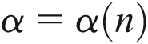 on the p-value when n increases. This approach fails to provide a working and logical principle from which this bound (or sequence of bounds)
 should be chosen. For instance, the article objects that because “of the large sample size, it is often judicious to choose a small type I error, say
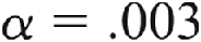 ” (78), when this argument simply points at the arbitrariness of this numerical value. In the specific setting of this example of Spanos (Reference Spanos2013), it is much worse, in that this bound could have been dictated by the data themselves since the observed p-value is equal to the nearby .0027. In addition, I find the argument of consistency unconvincing in that case since both the Bayes factor and the likelihood ratio tests are then consistent testing procedures.
In the Neyman-Pearson referential, there is a fundamental difficulty in finding a proper balance (or imbalance) between type I and type II errors, since such balance is not provided by the theory, which settles for the suboptimal selection of a fixed type I error. In addition, the whole notion of power, while central to this referential, has arguable foundations in that this is a function that inevitably depends on the unknown parameter  . In particular, the power decreases to the complement of the type I error at the boundary between the null and the alternative hypotheses in the parameter set. For instance, referring to Spanos’s (Reference Spanos2013, 87) arguments, giving a meaning to the definition of severity (eq. [25])

where x 0 is the observable and  should be
 , seems impossible. The third argument, “
 is false,” that conditions this probability statement makes no sense without a prior distribution on the parameter set.Footnote 14 Even the corrected version

depends on the choice of the particular alternative  or has to be seen as the power function, which, like the risk function (see, e.g., Berger Reference Berger1985), prohibits most comparisons in a frequentist framework.
As discussed further in section 2.2, if we abstain from discussing the genuine difficulty in setting a joint prior distribution over two distinct parameter spaces, following a standard Bayesian approach with a flat (uniform) prior distribution on the binomial probability inferred in Spanos (Reference Spanos2013, 80) leads to a Bayes factor of 8.115. Although this quantity is larger than one, the calibration of the discrepancy from this threshold constitutes the central difficulty in using Bayes factors toward decision making, Jeffreys’s (Reference Jeffreys1939) scale being highly formal despite being often referenced (Kass and Wasserman Reference Kass and Wasserman1996).
3.3. Defending Severity
Spanos (Reference Spanos2013) rebounds on the failures (or fallacies?) of all three main approaches to address the difficulties with the Jeffreys-Lindley paradox to advocate his own criterion, the “postdata severity evaluation” introduced in Mayo and Spanos (Reference Mayo and Spanos2004).Footnote 15 I recall that a “hypothesis H passes a severe test” if the data agree with H and if it is highly probable that data not produced under H agree less with H (Spanos Reference Spanos2013, 86). While this sounds like a reasonable desiderata, the notion of severe tests has been advocated by Mayo and Spanos (Reference Mayo and Spanos2004) over the past years, but it has not yet made a dent on the theory or on the practice of statistical testing. As exemplified by the article (see, e.g., table 1, 88, and the discussion surrounding it), this solution requires more (user-based) calibration than the regular p-value, and it is thus bound to confuse practitioners. Indeed, the severity evaluation as explained in Spanos (Reference Spanos2013, 87) implies defining for each departure from the null, rewritten as 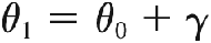 , the probability that a data set associated with this parameter value “accords less with
 than x 0 does.”Footnote 16 (Note that, as discussed in n. 15, the two-sided alternative has been turned postdatum into a one-sided version. This is no more acceptable than stating that the data always support more the value at the maximum likelihood then at the null.)
The notion of severity is therefore a mix of p-value and of type II error that is supposed to “provide the ‘magnitude’ of the warranted discrepancy from the null” (Spanos Reference Spanos2013, 88), that is, to decide about how close (in distance) to the null we can get and still be able to discriminate the null from the alternative hypotheses “with very high probability” (86). The description found in section 6 of Spanos (Reference Spanos2013) implies a rejection of H 0 for the data at hand, on the basis of the comparison of the p-value with an acceptance bound, as in Fisher’s perspective, followed by an assessment of “the largest discrepancy  from H 0 warranted by data x 0,” which derives a boundary parameter value
 from a severity level, .9 say. This amounts to selecting a minimal power or maximal type II error and checking for the corresponding discrepancy to be “substantively significant” (88), an assessment provided by the user and thus defeating the original purpose of the approach. The error statistical approach is therefore ineffective as an operational tool because of this double calibration that is required from the user. Once more, as detailed in Spanos (Reference Spanos2013), the value of this closest discrepancy
 —which is thus a bound on where we can discriminate between H 0 and H 1 for a given sample size n—does depend on another arbitrary tail probability, the “severity threshold,”

introduced in equation (25). This tail probability has to be chosen by the user without being more intuitive or less subjective than the initial acceptance bound on the p-value.Footnote 17 Furthermore, once the resulting discrepancy  is found, whether it is far enough from the null is a matter of informed opinion since, as duly noted by Spanos (Reference Spanos2013), whether it is “substantially significant … pertains to the substantive subject matter” (88), implying once again some sort of loss function or prior information that the article fails to acknowledge.Footnote 18
3.4. Falling Afoul of the Fallacy of Rejection
In connection with the special meaning of the value  and with the argument of the fallacy of rejection, mentioned by Spanos (Reference Spanos2013) as associated with the p-value, several parts of his discussion of the Bayesian approach state (see, e.g., 81) that other values of
 are supported and even better supported by the data than the null value
 . This is a surprising argument as (a) it pertains to the construction of Bayesian credible intervals but not to testing, and (b) it is a direct illustration of the “fallacy of rejection” in that rejecting (or not) H 0 does not bring evidence in favor of a particular value of
 . While it is correct that the observed data
 do “favor certain values [of the parameter] more strongly” (81) than
 , those values are (a) driven by the data (i.e., will vary from one repetition of the statistical experiment to the next) and (b) of no particular relevance for conducting a test, meaning that the experimenter or the scientist behind the experiment had not expressed a particular interest in those values before they were exposed by the data. The tested value,
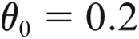 , say, is chosen before the experiment because it has some special meaning for the problem or the theory at hand. The fact that the likelihood, the posterior, or both are larger in other values of
 does not constitute “conflicting evidence” (82) against the fact that the null hypothesis holds. It simply reflects on the property that the likelihood function is a random function of the parameter
 , whose mode also varies with the data and is almost surely not located at the true value of the parameter. Since this is mathematically obvious, I find it astounding that it can be used as a logical argument against some statistical approaches to testing.
4. Toward a Resolution of the Bayesian Version of the Paradox
While the divergence between the frequentist and the Bayesian answers is reflecting on the difference between the paradigms in terms of purpose and evaluation, rather than condemning one of the approaches as implied by Spanos (Reference Spanos2013), the (Bayesian) debate about constructing limiting Bayes factors or posterior probabilities that include improper prior modeling stands both open and relevant. DeGroot’s (Reference DeGroot1982, 337) warning that “diffuse prior distributions … must be used with care” has now been impressed upon generations of students, and it is indeed a fair warning. There remains nonetheless a crucial need to produce assessments of null hypotheses from a Bayesian perspective and under limited prior information, once again without any incentive whatsoever to mimic, reproduce, or even come close to frequentist solutions like p-values.
Robert (Reference Robert1993) suggested selecting the prior weights of the two hypotheses, 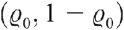 toward compensating for the increased mass produced by the alternative hypothesis prior.Footnote 19 While the solution therein produced results that brought a numerical proximity with the (standard) p-value, its construction is flawed from a measure-theoretic perspective since the determination of the weights involves the value of the prior density
 at the point-null value
 ,

while a probability density is only defined almost everywhere. This difficulty is shared by the Savage-Dickey paradox representing the Bayes factor solely in terms of the prior density under the alternative hypothesis (Robert and Marin Reference Robert and Marin2010).Footnote 20 I nonetheless second this opinion that the degree of freedom represented by the prior weight  in the Bayesian formalism should not be neglected to overcome the difficulty in using improper priors.Footnote 21
Among several available resolutions (see, e.g., Robert Reference Robert2001, chap. 5), a further step worth mentioning is Berger, Pericchi, and Varshavsky’s (Reference Berger, Pericchi and Varshavsky1998) partial validation of the use of identical improper priors on the nuisance parameters, a notion already entertained by Jeffreys (see the discussion in Robert et al. Reference Robert, Chopin and Rousseau2009, sec. 6.3). While arguing about the case of the “same” constant in both models as validating picking the “same” improper prior for both models has neither mathematical nor statistical validation, relying on the same prior quite handily eliminates the major thorn in the side of Bayesian testing of hypotheses. As demonstrated in Marin and Robert (Reference Marin and Robert2007) and Celeux et al. (Reference Celeux, Anbari, Marin and Robert2012), it allows in particular for the use of a partly improper g-prior in linear and generalized linear models (Zellner Reference Zellner1986).Footnote 22
A last step toward the incorporation of improper priors within the Bayesian testing paraphernalia is the recent investigation of the use of score functions S(x, m) that extend the standard log score function associated with the Bayes factor:

where mi is the prior predictive associated with model  . Indeed, there exists a whole family of proper scoring rules that are independent from the normalizing constant of the prior predictive (Parry, Dawid, and Lauritzen Reference Parry, Dawid and Lauritzen2012) and can thus be used on improper priors as well. For instance, Hyvärinen’s (Reference Hyvärinen2005) is one of these scores. While the scores are delicate to calibrate (i.e., the magnitude of S(x, m 1) − S(x, m 2) is not absolute), they provide a consistent method for selecting models (Berger Reference Berger1985) and avoid the delicate issue of selecting priors that differ for model selection and for regular inference (conditional on the model). This is why Sprenger (Reference Sprenger2013) advises replacing the Bayes factor with a logarithmic score, rewritten as
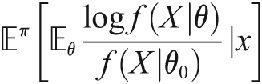
and compared with an acceptance bound. The Kullback-Leibler divergence used in this score is utterly natural in terms of evaluating the impact of replacing one distribution with the other. And, as stressed by Sprenger (Reference Sprenger2013), “we are less interested in the truth of H 0 than in its usefulness” (6). The use of this score, however, requires the choice of an acceptance bound, whose calibration is not provided by the theory.
5. Reflections
Even though I almost uniformly disagree with the presentation of the Jeffreys-Lindley paradox found in his article, I am most grateful to Aris Spanos for rekindling my interest in the paradox and inducing me to spell out my thoughts on the topic in an organized manner. This article has provided a perspective on the foundations of Bayesian inference toward testing statistical hypotheses, including the recovery of (some) improper priors for this purpose, and on the reasons why the severity-based approach of Mayo and Spanos (Reference Mayo and Spanos2004) fails as a convincing alternative to and criticism of the existing branches of statistical hypothesis testing. I argued against the notion that the discrepancy between frequentist and Bayesian procedures was a paradox, even when occurring asymptotically. I also disputed the common argument that the Jeffreys-Lindley paradox prohibits the use of improper priors and instead called for the use of score and predictive procedures in this context.
The appeal of great paradoxes is to address foundational issues in a field, either to reinforce the arguments in favor of a given theory or, on the opposite side, to cast serious doubts on its validity.Footnote 23 The fact that the Jeffreys-Lindley paradox is still discussed in papers (as exemplified by Spanos [Reference Spanos2013] and Sprenger [Reference Sprenger2013]) and blogs, by statisticians and nonstatisticians alike, is a testimony to its impact on the debate about the deepest foundations of statistical testing. The irrevocable opposition between frequentist and Bayesian approaches to testing and also the persistent impact of the prior modeling in this case are fundamental questions that have not yet met with definitive answers. And they presumably never will for, as aptly put by Lad (Reference Lad2003, 1), “the weight of Lindley’s paradoxical result … burdens proponents of the Bayesian practice.” However, this is a burden with highly positive features in that it paradoxically drives the field to higher grounds, like the devising of novel decisional tools assessing deeper and better the impact of a particular model choice, when compared with the Bayes factor solution producing a unique number.Footnote 24
 above.
 associated with the parameter
 , where
 is determined by the severity criterion, detailed in sec.
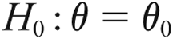 , the sign of
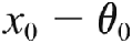 “indicates the relevant direction of departure from H 0” (86). First, random variables may take values on both sides of
 for most values of
 . Second, the fact that one is testing H 0 against a two-sided or a one-sided alternative hypothesis pertains to the motivation of the test, not to the direction suggested by the data. The contentious modification of the testing setting once the data are observed is a major issue with Spanos’s (
 , complement to a probability cumulative distribution function in
 , its most natural interpretation would be of a Bayesian nature, the bound being then a prior quantile. However, this solution is quite unlikely to meet with the author’s approval.
 that is continuous at
 so that
 is uniquely defined. It, however, does not escape controversy as it equates the values of two density functions under two orthogonal measures, the Lebesgue measure and a Dirac measure.


