Implications
Analysis shows that the pairwise tagSNP selection approach based on linkage disequilibrium information is a universal procedure, which is independent of the reference population structure. This has an impact on microarray construction that does not need to be designed specifically for each population.
Introduction
In the last decade, more and more genetic polymorphisms are being discovered for all domestic species, including cattle. From all kinds of genetic variation single nucleotide polymorphisms (SNPs) play the main role as variation factors (LaFramboise, Reference LaFramboise2009) and are widely used as genetic markers in genetic studies (Barendse et al., Reference Barendse, Reverter, Bunch, Harrison, Barris and Thomas2007). SNP information is also used by many countries to predict genomic breeding values (Calus, Reference Calus2010). In dairy cattle, it has been shown that estimating breeding values based on marker information can reduce costs of selection by up to 92% (Schaeffer, Reference Schaeffer2006).
Linkage disequilibrium (LD) expresses a deviation of random SNP alleles’ association (Boehnke, Reference Boehnke2000). Due to LD, one or more SNPs can be represented by a single tagSNP, reducing the number of SNPs needed for further analyses with a minimal decrease of data set informativeness. This is because a tagSNP subset covers most of the variation in the genome (LaFramboise, Reference LaFramboise2009). SNP arrays such as the Illumina BovineSNP50 were designed for population-wide use and are not constructed for any specific population (Matukumalli et al., Reference Matukumalli, Lawley, Schnabel, Taylor, Allan, Heaton, O'Conell, Moore, Smith, Sonstegard and Van Tassell2009). The main idea behind tagging the array is to adjust it to the population being analysed.
Until now, no tagSNP selection studies on Polish Holstein-Friesian (HF) population have been performed. Furthermore, no studies have compared the influence of a reference population structure on tagSNP selection. Therefore, the aim of this study is to select tagSNPs in Polish HF cattle population and to check whether relationship structure influences tagSNP selection results.
Material
Animals
The animals comprised representative 1228 Polish HF bulls born between 1997 and 2003. The bulls were related with the coefficient of relationship varying between 0.00 and 0.65 with a mean of 0.03 ± 0.04 and a median of 0.02. The average coefficient of relationship per bull varied between 0 and 0.06 with a mean of 0.03 ± 0.08 and a median of 0.03. The inbreeding coefficient of the animals calculated over 10 generations varied between 0.00 and 0.13 with a mean of 0.01 ± 0.01 and a median of 0.004.
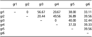
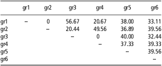
In order to investigate whether tagging depends on population parameters, six subsets of data were formed each consisting of 450 individuals. The first group (gr1) comprised animals having low average coefficients of relationship (between 0.00 and 0.03). The second group (gr2) comprised animals having high average coefficient of relationship (between 0.03 and 0.06). The third group (gr3) comprised animals having low coefficients of inbreeding (between 0.000 and 0.002). The fourth group (gr4) comprised animals having high coefficients of inbreeding (between 0.008 and 0.134). Two random groups (gr5 and gr6) were also created. The reference group comprised all 1228 bulls. The groups were used for tagSNP selection. The percentage of common individuals between groups is summarised in Table 1. Group gr1 and gr2 as well as gr3 and gr4 contain no common individuals. The largest number of common animals occurs between gr1 and gr3 (56.67%) as well as between gr2 and gr4 (49.56%).
The percentage of common individuals between groups
SNP genotypes
Each bull was genotyped with the BovineSNP50 BeadChip version 1 (Illumina Inc., San Diego, CA, USA) consisting of 54 001 SNPs. 52 336 (96.9%) of the SNPs were mapped to chromosomes, while the remainder, consisting of 1665 SNPs had no information regarding location and were, therefore, excluded from further analysis. The number of SNPs varies from 3343 for BTA1 to 747 for BTX. The density distribution of a distance between two adjacent SNPs was estimated using kernel estimators with Gaussian kernel implemented in the R software (R Development Core Team, 2010). Supplementary material 1 shows density functions estimated for all chromosomes. Beside BTX, all chromosomes show evenly spaced SNPs (narrow peak) with a small number of outliers (long tail). Mean distance (red line) spans from 44 686 bp for BTA25 to 118 807 bp for BTX. On average (genome-wide) the estimated distance between adjacent SNPs was 51 728 bp.
Minor allele frequency (MAF) varies from 0.00 to 0.50. Mono-allelic SNPs (MAF = 0) are over-represented, while the other classes are represented uniformly. The average MAF across all chromosomes is 0.227 ± 0.0088, varying between 0.213 for BTX and 0.245 for BTA25.
Methods
TagSNP selection
The Tagger software (de Bakker et al., Reference de Bakker, Yelensky, Pe'er, Gabriel, Daly and Altshuler2005) implemented in Haploview (Barrett et al., Reference Barrett, Fry, Maller and Daly2004) was used to select tagSNPs using the greedy pairwise tagging algorithm as described by Carlson (Carlson et al., Reference Carlson, Eberle, Rieder, Quian, Krygulak and Nickerson2004). TagSNPs were selected based on r 2 ⩾ 0.8 (representing pairwise LD between SNPs) and MAF ⩾ 0.01.
Determining the structure of LD blocks
Haploview (Barrett et al., Reference Barrett, Fry, Maller and Daly2004) was used for LD block selection. Following Gabriel et al. (Reference Gabriel, Schaffner, Nguyen, Moore, Roy, Blumenstiel, Higgins, DeFelice, Lochner, Faggart, Liu-Cordero, Rotimi, Adeyemo, Cooper, Ward, Lander, Daly and Altshuler2002), SNP pairs are in ‘strong LD’, if the one-sided upper 95% confidence bound on D′ is >0.98 (no historical recombination) and the lower bound is above 0.7. However, ‘strong evidence for historical recombination’ is if the upper confidence bound on D′ is <0.9. SNPs with MAF > 0.05, which belongs to these two categories, are considered to be informative. The confidence bounds on D′, rather than the point estimates of D′ are used because the D′ values are known to fluctuate upward when a small number of samples or rare alleles are examined. The confidence limits were determined by calculating the probability of the observed data for all possible values of D′, from which an overall probability distribution was determined. The proportion of informative pairs in strong LD in the block must be at least 95%.
Results
Comparisons of tagSNP selection thresholds
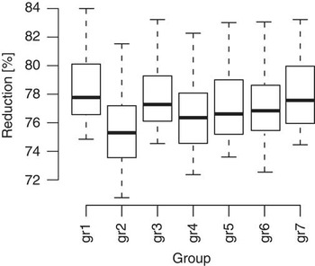
TagSNP selection was performed in six subgroups. For autosomes reduction (the percentage of tagSNPs estimated from the original set of SNPs) varies between 74.8% (BTA7) and 84.0% (BTA28) for gr1; between 70.7% (BTA7) and 81.5% (BTA28) for gr2; between 74.5% (BTA7) and 83.2% (BTA28) for gr3; between 72.4% (BTA7) and 82.3% (BTA28) for gr4; between 73.6% (BTA16) and 83.0% (BTA28) for gr5; and between 72.6% (BTA7) and 83.0% (BTA28) for gr6. The average reduction over all groups and all autosomes is 77.2 ± 2.66%. Figure 1 shows the differences in reduction between subgroups observed for all autosomes. The highest reduction over all autosomes is 73.82% (gr2) and is higher than the reduction observed for the reference data set, whereas the lowest reduction of 76.95% obtained for gr1 is very similar to the reduction in the reference data. Only small differences in the number of selected tagSNPs are observed between gr4, gr5 and gr6. In supplementary material 2, the reduction is compared over subgroups and the reference population (gr7) by fitting a straight line across values for autosomes. The linear regression coefficient fitted to the data varies between 0.88 (gr1 to gr7 and gr3 to gr7) and 1.05 (gr2 to gr7), and is not significantly different from the value of 1 expected under no differences in reduction between groups.
Reduction in different subgroups. TagSNP % from the original SNP set. BTX was excluded.

Comparisons of tagSNP sets
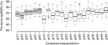
In order to investigate the degree of similarity between tagSNP sets selected for different groups a percentage of identical tagSNPs was identified (Figure 2). For autosomes, the percentage of identical tagSNPs varies from 88.2% between gr1 and gr2 for BTA8 to 97.9% between gr3 and gr5 for BTA25. The average similarity is 93.8 ± 1.69%.
Percentage of common tagSNPs between subgroups. Comparisons between sub-populations and the reference population are marked grey. BTX was excluded.

LD blocks
LD blocks are used to indicate the pieces of DNA that are inherited together with high probability. LD blocks are selected on each chromosome, but on BTX it is not possible to determine blocks. The total number of discovered blocks is 1163. The lowest number (8) is for BTA27 and BTA28 and the highest (97) is for BTA1. On average, the block length is 170.8 kbp, but for chromosomes taken separately it varies from 123.9 kbp for BTA22 to 199.3 kbp for BTA5. Moreover, the minimum block size is 0.5 kbp and the maximum is 499 kbp. The total length of blocks per chromosome varies from 17 357.5 kbp for BTA1 to 1160.5 kbp for BTA28. Chromosome coverage (the percentage of total block length per chromosome) varies from 11.5% for BTA6 to 2.52% for BTA28. The genome-wide coverage is 7.17%.
Discussion
Ding and Kullo (Reference Ding and Kullo2007) distinguished between haplotype tagging and pairwise tagging as two different approaches. Although Qanbari et al. (Reference Qanbari, Pimentel, Tetens, Thaller, Lichtner, Sharifi and Simianer2010) used the same array and breed; they obtained a different number of tagSNPs as compared with our study. It is unclear whether this was caused by the differences in the genetic structure of the populations studied, or in the methodology of tagSNP selection. The approach adopted by Qanbari et al. (Reference Qanbari, Pimentel, Tetens, Thaller, Lichtner, Sharifi and Simianer2010) was first to estimate haplotypes and then to use tagger to identify tagSNPs. This is a mixture of a haplotype and pairwise tagging. Our study is based entirely on the pairwise tagging approach. That is why the results of the two studies cannot be directly compared. Khatkar et al. (Reference Khatkar, Zenger, Hobbs, Hawken, Cavanagh, Barris, McClintock, McClintock, Thomson, Tier, Nicholas and Raadsma2007) and Marques et al. (Reference Marques, Schnabel, Stothard, Kolbehdari, Wang, Taylor and Moore2008) also used pairwise tagging, but on smaller data sets.
Tagging is a crucial part of SNP assay (Ke et al., Reference Ke, Miretti, Broxholme, Hunt, Beck, Bentley, Deloukas and Cardon2005). It results in significant time and cost savings. Smaller arrays are cheaper to construct and easier to work with (Ke et al., Reference Ke, Miretti, Broxholme, Hunt, Beck, Bentley, Deloukas and Cardon2005). The downside of tagging is the possibility that some variation may not be covered by tagSNPs. Since the first genome-wide LD analysis of the bovine genome based on SNPs was performed by Khatkar et al. (Reference Khatkar, Zenger, Hobbs, Hawken, Cavanagh, Barris, McClintock, McClintock, Thomson, Tier, Nicholas and Raadsma2007), it has been clear that the number of SNPs available for cattle on commercial microarray is not sufficient to cover the entire variance in the cattle genome (e.g. single nucleotide variance, copy number variance and microsatellite variance). Khatkar et al. (Reference Khatkar, Zenger, Hobbs, Hawken, Cavanagh, Barris, McClintock, McClintock, Thomson, Tier, Nicholas and Raadsma2007) proposed 30 to 50 kbp spacing between two tagSNPs to achieve full variation coverage. They assumed that a microarray consisting of 200 000 to 250 000 SNPs would be sufficient. Those authors used an Affymetrix 10k array (Affymetrix Inc., Santa Clara, CA, USA) enhanced by additional SNPs. Although Gautier et al. (Reference Gautier, Faraut, Moazami-Goudarzi, Navratil, Foglio, Grohs, Boland, Garnier, Boichard, Lathrop, Gut and Eggen2007) used a set of SNPs that was 10 times smaller than used by Khatkar et al. (Reference Khatkar, Zenger, Hobbs, Hawken, Cavanagh, Barris, McClintock, McClintock, Thomson, Tier, Nicholas and Raadsma2007); they proposed a microarray containing one tagSNP per 10 kbp which would result in ∼300 000 tagSNPs. This estimate was later supported by Kim and Kirkpatrick (Reference Kim and Kirkpatrick2009) and now by our results. McKay et al. (Reference McKay, Schnabel, Murdoch, Matukumalli, Aerts, Coppieters, Crews, Neto, Gill, Gao, Mannen, Stothard, Wang, Van Tassell, Williams, Taylor and Moore2007), Prasad et al. (Reference Prasad, Schnabel, McKay, Murdoch, Stothard, Kolbehdari, Wang, Taylor and Moore2008) and Sargolzaei et al. (Reference Sargolzaei, Schenkel, Jansen and Schaeffer2008) arrived at completely different conclusions. They claimed that the minimum array for association study should consist of SNPs < 70 kbp apart. This would result in ∼50 000 SNP for such array. Villa-Angulo et al. (Reference Villa-Angulo, Matukumalli, Gill, Choi, Van Tassell and Grefenstette2009) used much larger set of SNPs. They proposed an assay of 30 000 SNPs for GWAS and 580 000 to construct the whole-genome haplotype-block structure. Qanbari et al. (Reference Qanbari, Pimentel, Tetens, Thaller, Lichtner, Sharifi and Simianer2010) suggested that 75 000 SNPs with MAF ⩾ 0.05 or 50 000 SNPs with MAF ⩾ 0.15 are useful for GWAS. For genomic evaluation, Banos and Coffey (Reference Banos and Coffey2010) and de Roos et al. (Reference de Roos, Hayes, Spelman and Goddard2008) proposed 300 000 SNPs. However, this number is dependent on trait heritability and mode of inheritance (pure polygenic, oligogenic).
The number of blocks identified in this study is much higher than the number of LD blocks reported in previous studies. In this study, 1163 blocks were identified. This is considerably more than the 727 LD blocks identified by Khatkar et al. (Reference Khatkar, Zenger, Hobbs, Hawken, Cavanagh, Barris, McClintock, McClintock, Thomson, Tier, Nicholas and Raadsma2007) who used a smaller array, and 712 blocks identified by Qanbari et al. (Reference Qanbari, Pimentel, Tetens, Thaller, Lichtner, Sharifi and Simianer2010) based on the same microarray used in this study. However, the mean and median block sizes obtained in this study (170 kbp, 148 kbp) are very similar to the values reported by Qanbari et al. (164.0 kbp, 144.0 kbp), whereas Khatkar et al. (Reference Khatkar, Zenger, Hobbs, Hawken, Cavanagh, Barris, McClintock, McClintock, Thomson, Tier, Nicholas and Raadsma2007) obtained much lower values (69.7 kbp, 3.9 kbp). Consequently, the German HF population analysed by Qanbari et al. (Reference Qanbari, Pimentel, Tetens, Thaller, Lichtner, Sharifi and Simianer2010) has lower genome coverage by blocks (4.67%) as compared with the Polish HF population (7.17%). In addition, the Australian HF population analysed by Khatkar et al. (Reference Khatkar, Zenger, Hobbs, Hawken, Cavanagh, Barris, McClintock, McClintock, Thomson, Tier, Nicholas and Raadsma2007) had a smaller coverage (2.27%).
LD dynamics can be considered long-term across tens of generations as well as short-term over a decade. The differences between the Polish and German populations may be a result of these two possible schemes. To look at these respectively: (i) with the exception of the last few decades, these two populations have been effectively isolated (long-term scheme); and (ii) there have been different selection approaches over the last decade – more traits were selected in the German HF (short-term scheme). In the last three decades, selection has been significantly accelerated because of artificial insemination (a top bull may now have thousands of daughters in many countries).
LD blocks may be treated as a measure of the quality of a microarray (Matukumalli et al., Reference Matukumalli, Lawley, Schnabel, Taylor, Allan, Heaton, O'Conell, Moore, Smith, Sonstegard and Van Tassell2009; Villa-Angulo et al., Reference Villa-Angulo, Matukumalli, Gill, Choi, Van Tassell and Grefenstette2009). The better the coverage, the more genetic variation captured by the blocks. Obviously, 100% coverage cannot be achieved because of factors such as crossing-over. Still, the coverage of the cattle genome is marginal.
It is worth mentioning that the sample size is an important factor for accurate r 2 estimation and consequently for tagSNP selection. Khatkar et al. (Reference Khatkar, Nicholas, Collins, Zenger, Cavanagh, Barris, Schnabel, Taylor and Raadsma2008) proposed a sample size of 75 as the smallest usable number for r 2 estimation. The sample size used in this study was more than 24 times larger. Reliable tagSNP selection was, therefore, ensured in this study.
Conclusions
Our study revealed that the vast majority of tagSNPs was shared between subgroups of different population parameters (gr1 to gr6). The obtained results show that in order to generate a tagSNP set valid for the whole population, there is no need to genotype a large number of reference animals. The pairwise tagSNP selection approach based on LD information is a universal procedure, which is independent of the reference population structure. On the other hand, the currently most commonly used SNP array in dairy cattle (Illumina BovineSNP50) does not provide sufficient SNP density to allow for a reasonable selection of tagSNPs – since the LD blocks identified by the SNPs only cover 7% of the whole genome. Furthermore, there is no established method for tagSNP selection. MAF and LD thresholds have to be set with common sense.