

Understanding the Electoral College is fundamental to understanding US presidential elections. Many students first encounter the concept of the Electoral College in an introduction course on American politics and subsequently revisit it in more advanced courses. Most students are familiar with the two key features of the Electoral College. First, the number of Electoral College votes allocated to a state is determined by the House-seats-plus-two formula. For example, Massachusetts, with nine House seats after the 2020 US Census, had 9+2=11 Electoral College votes in the 2024 presidential election. Second, 48 of 50 states as well as Washington, DC, use a winner-take-all system for translating popular votes to Electoral College votes. For example, Joseph Biden won 52.4% of the popular votes in Minnesota in 2020 and, as a result, received all 10 of the state’s Electoral College votes.Footnote 1 In recent decades, a seemingly befuddling phenomenon is that a presidential candidate can win the popular vote (as the plurality winner) but lose the Electoral College vote and therefore lose the presidency. The most recent examples took place in 2000 and 2016, as shown in table 1.Footnote 2
Presidential Election Inversions in 2016 and 2000

Table 1 Long description
The table contains five columns: Election Year, Candidate, Popular Vote Totals, Popular Vote percentage, and Electoral College Vote Totals.
For the 2016 election:
* Hillary R. Clinton (D) received 65,853,514 popular votes (48.18 percent) and 227 Electoral College votes.
* Donald J. Trump (R) received 62,984,828 popular votes (46.09 percent) and 304 Electoral College votes.
For the 2000 election:
* Al Gore (D) received 50,999,897 popular votes (48.38 percent) and 266 Electoral College votes.
* George W. Bush (R) received 50,456,002 popular votes (47.87 percent) and 271 Electoral College votes.
A footnote indicates that the total vote count includes votes for third-party candidates.
Note: *Total vote count includes votes for third-party candidates.
How does an election inversion occur?Footnote 3 Unfortunately, many students are not equipped to answer this question. Undergraduate textbooks on elections and voting often provide limited insight into the Electoral College as a two-stage preference aggregation system because the study of such mechanisms is concentrated primarily in the field of social choice theory.
Understanding election inversions in the Electoral College is important for two reasons. First, voter confidence in the US presidential election process has reached new lows in recent years (Enders et al. Reference Enders, Uscinski, Klofstad, Premaratne, Seelig, Wuchty, Murthi and Funchion2021; Wilson and King-Meadows Reference Wilson and King-Meadows2016). When students do not understand how seemingly unfair outcomes such as election inversions can occur, their trust in the democratic process may erode further (Carey et al. Reference Carey, Helmke, Nyhan, Sanders, Stokes and Yamaya2022). Second, because the recent election inversions in 2000 and 2016 benefited Republicans and disadvantaged Democrats, students may perceive election inversions as inherently partisan. This perception could undermine discussions of electoral reform, because it creates the false impression that any Electoral College reform would advantage Democrats and harm Republicans (Aldrich, Reifler, and Munger Reference Aldrich, Reifler and Munger2014; Toll and Corona Reference Toll and Corona2024). The encouraging news is that voter education can help combat misconceptions and increase voter confidence (Gaudette et al. Reference Gaudette, Hill, Kousser, Lockhart and Romero2025; Lockhart et al. Reference Lockhart, Gaudette, Hill, Kousser, Romero and Uribe2024; Suttmann-Lea and Merivaki Reference Suttmann-Lea and Merivaki2023), especially when voter education precedes an election crisis (Winger et al. Reference Winger, Calfano, Vićić and Harknett2023). Thus, helping students better understand the Electoral College may have long-lasting positive impacts on voter confidence and civic engagement.
This article presents two models that use only foundational arithmetic to help undergraduates understand how a candidate can win the popular vote but lose the Electoral College vote. The models are accompanied by ready-to-use and customizable worksheets, included in the online appendix, with detailed answers and pedagogical notes. The article also discusses additional factors that contribute to election inversions, drawing from the social choice literature. The section on pedagogy offers suggestions for incorporating the models into an existing course.
This article presents two models that use only foundational arithmetic to help undergraduates understand how a candidate can win the popular vote but lose the Electoral College vote. The models are accompanied by ready-to-use and customizable worksheets, included in the online appendix, with detailed answers and pedagogical notes.
A survey study of the student-learning experiences from the Fall 2024 and Spring 2025 semesters demonstrated positive results. Students consistently reported that they found the models accessible and, after completing the worksheets, they better understood how election inversions happen and how US presidential elections work more broadly. Moreover, students reported an increased level of confidence in the integrity of US presidential elections and in democracy in America. These responses align with existing literature suggesting that educational information about the election process can positively influence voter trust, demonstrating the pedagogical and civic value of incorporating these models into American politics courses.
The models and worksheets presented in this article are active-learning tools: they challenge students with a puzzle, require them to work toward discovering the answers themselves, and facilitate peer-to-peer discussion and interaction. Active-learning pedagogy has become a growing trend in higher education because of its demonstrated value in increasing student learning, especially in science, technology, engineering, and mathematics (STEM) disciplines (Freeman et al. Reference Freeman, Eddy, McDonough, Smith, Okoroafor, Jordt and Wenderoth2014). Active-learning strategies, especially simulations, have received increasing attention in political science education as well (Asal and Blake Reference Asal and Blake2006; Wedig Reference Wedig2010). Research reveals that simulations improve student engagement, knowledge retention, and metacognitive skills, among other benefits (Jones and Bursens Reference Jones and Bursens2015; Shellman and Turan Reference Shellman and Turan2006).
Although active-learning activities exist for American politics courses, they are fewer in number than in international relations and comparative politics courses, where activities such as Model UN and Model EU readily lend themselves to student-centered active learning (Baranowski Reference Baranowski2006; Kammerer and Higashi Reference Kammerer and Higashi2021). Pedagogical tools for teaching about the Electoral College typically emphasize constitutional design (National Constitution Center n.d.); voter participation and mobilization (Brew Reference Brew2025; McGowan-Kirsch Reference McGowan-Kirsch2021); voter coalition building through mapping exercises (270towin n.d.); and reform debate (PBS NewsHour Classroom 2024). To our knowledge, there is no published work in political science pedagogy that explicitly explains the social choice theory underlying the Electoral College vote. The teaching and learning tools described in this article fill this gap by meaningfully expanding the set of active-learning strategies available for American politics courses.
US PRESIDENTIAL ELECTION INVERSION: MODEL 1
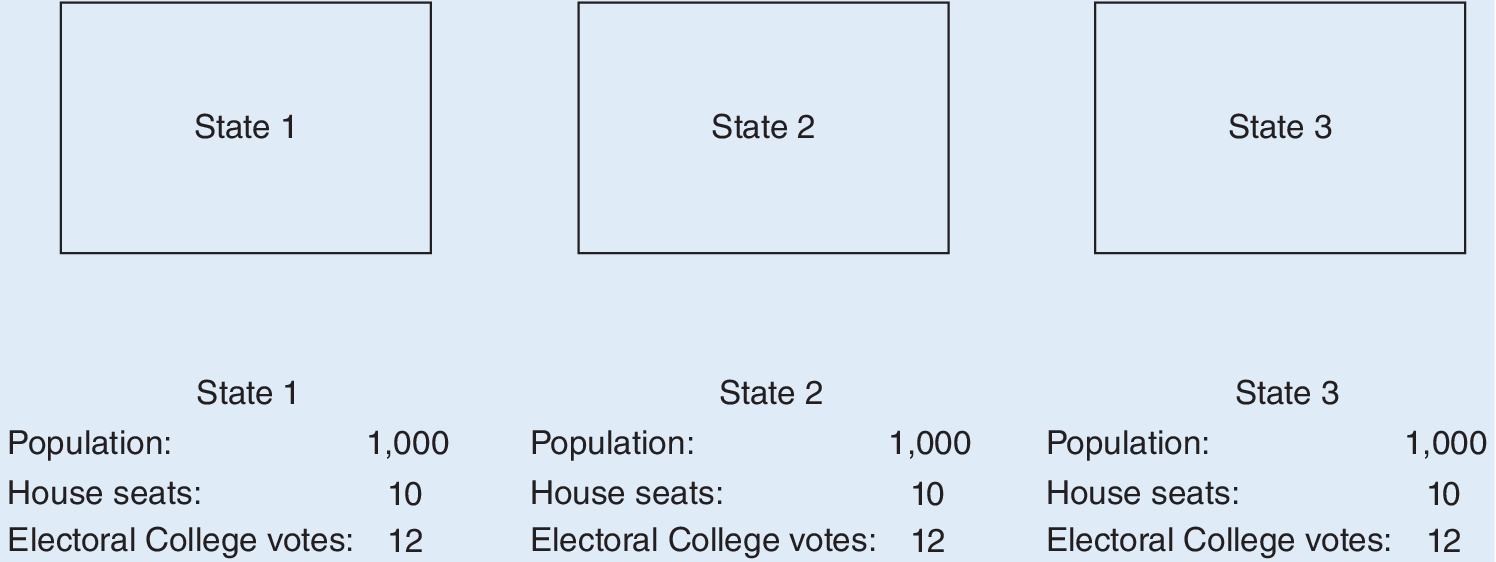
Model 1 begins with a simplified electoral map, shown in figure 1. The map consists of three states with the same population and apportionment number. The allocation of the states’ Electoral College votes follows the House-seats-plus-two rule. The allocation of the candidates’ Electoral College votes follows the winner-take-all system determined by the popular vote. The final election outcome is determined by the candidates’ Electoral College votes, following the simple-majority rule. In a two-candidate election in which everyone votes, candidate A wins 55% of the popular votes in states 1 and 2 and 30% in state 3. Candidate B wins the remaining popular votes.
Model 1 Setup

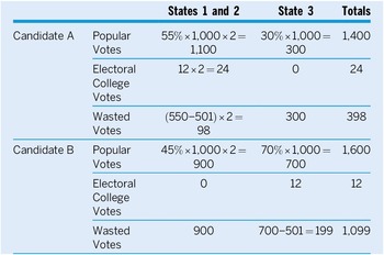
The electoral outcomes are presented in table 2. Candidate A wins the Electoral College vote but loses the popular vote, and candidate B wins the popular vote but loses the Electoral College vote. Because of the winner-take-all system, a candidate “wastes” all of their popular votes in losing states and all votes exceeding the minimum needed for a simple majority in winning states. In this example, candidate A wastes a total of 398 votes and candidate B wastes 1,099, contributing to an election inversion.
Electoral Outcome in Model 1

Table 2 Long description
The table is organized into five columns: Candidate, Metric, States 1 and 2, State 3, and Totals.
Candidate A data:
* Popular Votes: 55% times 1,000 times 2 equals 1,100 in States 1 and 2; 30% times 1,000 equals 300 in State 3; Total 1,400.
* Electoral College Votes: 12 times 2 equals 24 in States 1 and 2; 0 in State 3; Total 24.
* Wasted Votes: (550 minus 501) times 2 equals 98 in States 1 and 2; 300 in State 3; Total 398.
Candidate B data:
* Popular Votes: 45% times 1,000 times 2 equals 900 in States 1 and 2; 70% times 1,000 equals 700 in State 3; Total 1,600.
* Electoral College Votes: 0 in States 1 and 2; 12 in State 3; Total 12.
* Wasted Votes: 900 in States 1 and 2; 700 minus 501 equals 199 in State 3; Total 1,099.
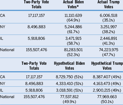
A closer examination of the results reveals that the winner-take-all system alone is sufficient for the election inversion in this case. Even without the House-seats-plus-two rule—that is, if each state has 10 instead of 12 Electoral College votes—candidate A still would win the Electoral College vote 20 to 10 while losing the popular vote. Because the winner-take-all system is not partisan, table 3 presents a hypothetical scenario in which a Republican suffers from more wasted votes, winning the popular vote but losing the Electoral College vote. If we were to increase Donald Trump’s two-party vote share in the 2020 presidential election in California, New York, and Illinois to 49%, as shown in table 3, he would have won the popular vote but still lose the Electoral College vote.
Hypothetical Case of Republican Election-Inversion Loss

Table 3 Long description
The table is divided into two vertical sections.
Section 1: Actual Biden and Trump Votes.
* C A: 17,117,157 total votes. Biden received 11,110,639 (64.9 percent). Trump received 6,006,518 (35.1 percent).
* N Y: 8,496,883 total votes. Biden received 5,244,886 (61.7 percent). Trump received 3,251,997 (38.2 percent).
* I L: 5,918,806 total votes. Biden received 3,471,915 (58.7 percent). Trump received 2,446,891 (41.3 percent).
* National: 155,507,476 total votes. Biden received 81,283,501 (52.3 percent). Trump received 74,223,975 (47.7 percent).
Section 2: Hypothetical Biden and Trump Votes.
* C A: 17,117,157 total votes. Biden received 8,729,750 (51 percent). Trump received 8,387,407 (49 percent).
* N Y: 8,496,883 total votes. Biden received 4,333,410 (51 percent). Trump received 4,163,473 (49 percent).
* I L: 5,918,806 total votes. Biden received 3,018,591 (51 percent). Trump received 2,900,215 (49 percent).
* National: 155,507,476 total votes. Biden received 77,537,812 (49.9 percent). Trump received 77,969,663 (50.1 percent).
Note: *Percentages in parentheses are two-party vote shares.
The hypothetical case proceeds as follows. In the 2020 presidential election, Joseph Biden performed well in California, New York, and Illinois, winning 64.9%, 61.7%, and 58.7% of the two‑party vote in those states, respectively. If we were to decrease his two‑party vote share to 51% in each of the three states, he still would have won the popular vote in each state; therefore, the Electoral College vote distribution would not change. Biden still would have received a national total of 306 Electoral College votes, and Trump still would have received 232. However, decreasing Biden’s two‑party share to 51% and increasing Trump’s to 49% in the three states would have changed the national popular-vote totals. In the actual 2020 election, Biden’s national popular-vote total was 81,283,501 and Trump’s was 74,223,975. In the hypothetical scenario in which Biden’s two‑party vote share in California, New York, and Illinois is reduced to 51%, Biden’s national popular-vote total would have been 77,537,812 and Trump’s would have been 77,969,663. In this case, Trump would have won the national popular vote but lost the Electoral College. This example demonstrates that a Republican candidate who narrowly loses in multiple populous states could accumulate an excess of wasted votes and therefore lose a presidential election through an election inversion.
US PRESIDENTIAL ELECTION INVERSION: MODEL 2
An analysis of wasted votes in the 2000 and 2016 presidential elections reveals that whereas Hillary Clinton indeed wasted more votes than Donald Trump in 2016, the same was not true in 2000, when George W. Bush wasted 29,003,302 popular votes compared to Al Gore’s 24,896,571.Footnote
4 How then to explain the election inversion in 2000? The answer lies in the House-seats-plus-two rule, which disproportionally benefits less-populous states by giving them greater electoral influence relative to their population size. To illustrate, consider the neighboring states of Washington and Idaho. After the 2020 US Census, Washington had 10 House seats and Idaho had two. Under the House-seats-plus-two rule, Washington received a
$ \frac{2}{10}=20\% $
 boost in its Electoral College vote and Idaho received a
$ \frac{2}{2}=100\% $
 boost. The advantage for less-populous states is especially pronounced in the Electoral College due to the positive skew of state Electoral College votes. After the 2020 US Census, the average state had 10.54 Electoral College votes, with a median of eight and a skewness of 2.68. This means that because nationally there are more smaller states, a candidate who wins more of these states can secure more Electoral College votes with fewer popular votes, thereby benefiting from the disproportionate allocation of Electoral College votes toward the smaller states.Footnote
5
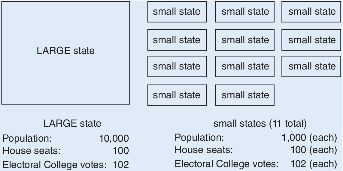
To illustrate the effect of the House-seats-plus-two rule, model 2 expands the electoral map to include one large state and 11 small states (figure 2). In a two-candidate election in which everyone votes, candidate A wins 60% of the popular votes in the large state, 55% in one small state, and 40% in the remaining small states. Candidate B wins the remaining popular votes. These electoral outcomes are shown in table 4.
Model 2 Setup

Electoral Outcome in Model 2

Table 4 Long description
The table is organized into columns for Large State, One Small State, Remaining 10 Small States, and Totals.
Candidate A data:
* Popular Votes: 60% times 10,000 equals 6,000 in Large State; 55% times 1,000 equals 550 in One Small State; 40% times 1,000 times 10 equals 4,000 in Remaining 10 Small States. Total: 10,550.
* Electoral College Votes: 102 in Large State; 12 in One Small State; 0 in Remaining 10 Small States. Total: 114.
* Wasted Votes: 6,000 minus 5,001 equals 999 in Large State; 550 minus 501 equals 49 in One Small State; 4,000 in Remaining 10 Small States. Total: 5,048.
Candidate B data:
* Popular Votes: 40% times 10,000 equals 4,000 in Large State; 45% times 1,000 equals 450 in One Small State; 60% times 1,000 times 10 equals 6,000 in Remaining 10 Small States. Total: 10,450.
* Electoral College Votes: 0 in Large State; 0 in One Small State; 120 in Remaining 10 Small States. Total: 120.
* Wasted Votes: 4,000 in Large State; 450 in One Small State; (600 minus 501) times 10 equals 990 in Remaining 10 Small States. Total: 5,440.
In this election, candidate A wins the popular vote but loses the Electoral College vote not because they waste more votes than candidate B. Rather, Candidate B is the one who wastes more popular votes, yet they still win the Electoral College vote by winning more of the small states, thereby benefiting from the extra boost. The literature confirms that whereas wasted votes contributed to the election inversion in 2016, the plus-two boost was a main cause for the election inversion in 2000 (Barthélémy, Martin, and Piggins Reference Barthélémy, Martin and Piggins2019; Cervas and Grofman Reference Cervas and Grofman2019).
To guide students through the logic and calculations of models 1 and 2, we created two worksheets (see the online appendix) with follow-up questions that encourage them to think deeper about the impact of election rules—not only votes—on electoral outcomes.
THE STUDENT-LEARNING EXPERIENCE STUDY
To understand the student-learning experience, we implemented surveys before and after the students completed the worksheets during six in-person sections of the “Introduction to US Government and Politics” course in the Fall 2024 and Spring 2025 semesters. Two aspects of the student-learning experience study are noteworthy. First, the study was conducted in a lower-division general-education course at a four-year regional public university, which tested the accessibility of the worksheets. A total of 295 student participated: 137 from three sections in Fall 2024 and 158 from three sections in Spring 2025. Among the participants, 284 were non-political science majors and 11 were political science majors. Additionally, 178 students were in their first or second year of college and 117 were in their third year or beyond (Li and Simpson Reference Li and Simpson2026).
A second notable aspect of the study is that it was conducted in the classroom of an instructor who was first introduced to the election-inversion models in Fall 2024. This context allowed for an assessment of whether the materials can be taught effectively by instructors without specialization in social choice theory. The models and worksheets were originally developed by a different faculty member who specializes in social choice theory and has used various iterations of the materials in courses for almost a decade. In contrast, the instructor involved in the student-learning experience study specializes in American political history. Although initially hesitant due to the quantitative nature of the models, the instructor recognized their pedagogical value. All students who participated in the survey study were taught by this newer instructor.
The student-learning experience study was conducted as follows. First, during a previous class session, the instructor gave the students an anonymous pre-survey that they filled out in person during class. Second, during the class session covering the Electoral College, the instructor gave a brief (10- to 15-minute) lecture on the history of the Electoral College and the two rules for allocating Electoral College votes, followed by distribution of the worksheets. In four of six sections, students were given one worksheet. In the other two sections, they were given both worksheets.
The initial verbal explanation of the worksheets was minimal because the instructor chose to let students read the instructions to learn how to fill them in. The students were informed that their work would not be graded but would be collected to count toward participation points. The use of calculators was permitted but the use of generative AI tools was not. The students were also allowed to discuss the worksheets with their classmates. After about 15 minutes, the instructor reviewed the worksheets with the students. Unfortunately, the instructor did not always have enough time to discuss the follow-up questions. Afterwards, the instructor collected the worksheets and gave the students an anonymous post-survey to complete.Footnote 6
WHAT WE FOUND: AN ACCESSIBLE AND POSITIVE LEARNING EXPERIENCE
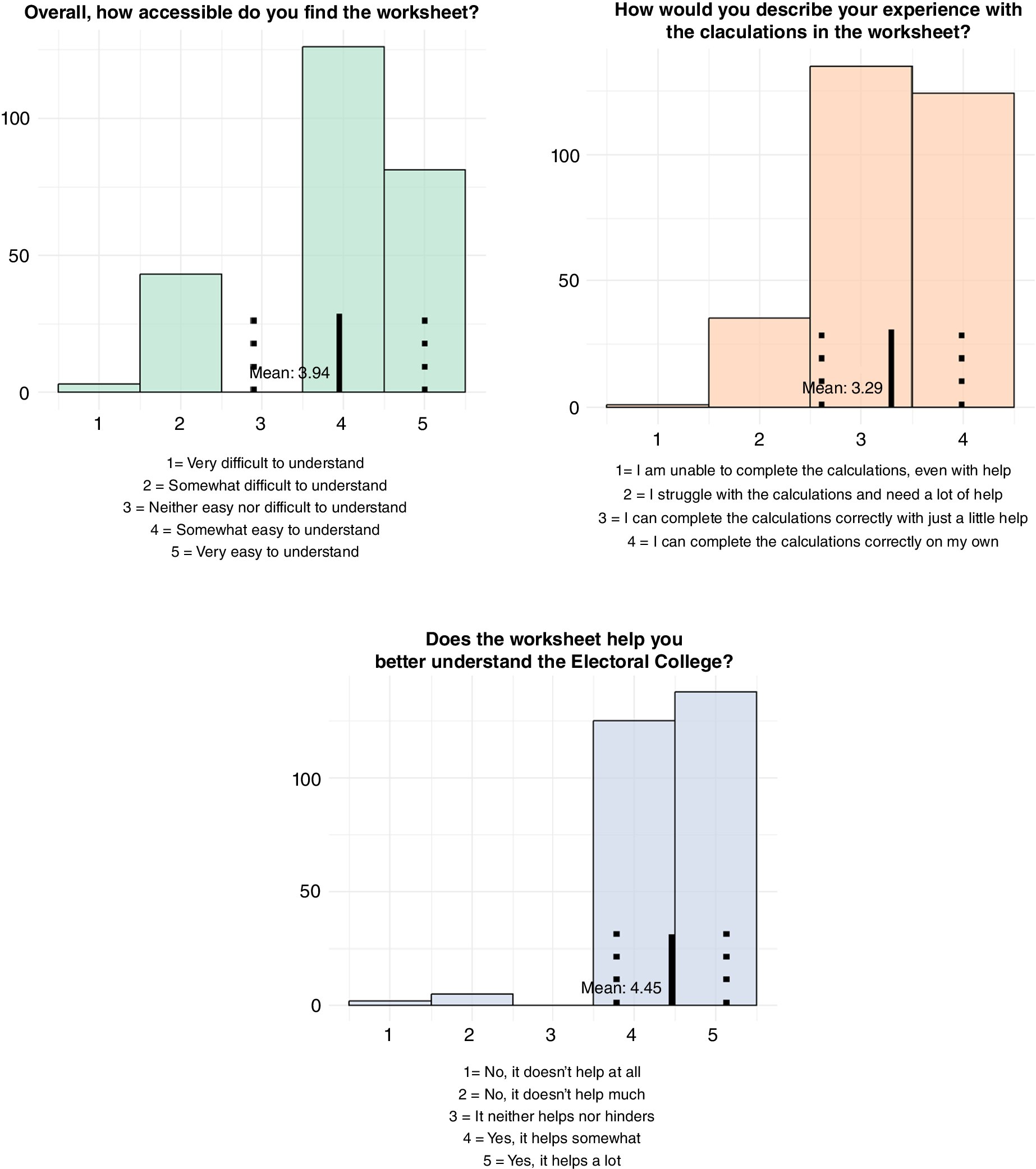
The results from the survey analysis were encouraging in two aspects. First, the students found the worksheets to be accessible, despite being given minimal instructions. Figure 3 shows that for the worksheet-accessibility question, the mean response was 3.94 (solid line), close to “4=somewhat easy to understand,” with a standard deviation of 1.06 (dashed line). For the ease-of-calculation question, the mean response was 3.29 (solid line), close to “3=I can complete the calculations correctly with just a little help,” with a standard deviation of 0.69 (dashed line). Second, the students generally found the learning experience to be helpful. When asked if the worksheet helped them better understand the Electoral College, they overwhelmingly responded that “it helps a lot” and “it helps somewhat.”
Student Perceptions of Accessibility and Helpfulness (Post-Survey Only)

Figure 3 Long description
A multi-panel figure containing three histograms.
Top-left panel: Overall, how accessible do you find the worksheet? The x-axis ranges from 1 to 5, where 1 is Very difficult to understand and 5 is Very easy to understand. The y-axis represents frequency from 0 to 100. Bars show a significant peak at 4 and 5. A vertical black line indicates a Mean of 3.94.
Top-right panel: How would you describe your experience with the calculations in the worksheet? The x-axis ranges from 1 to 4, where 1 is unable to complete even with help and 4 is able to complete correctly on my own. The y-axis represents frequency from 0 to 100. Bars show a high concentration at 3 and 4. A vertical black line indicates a Mean of 3.29.
Bottom panel: Does the worksheet help you better understand the Electoral College? The x-axis ranges from 1 to 5, where 1 is No, it doesn't help at all and 5 is Yes, it helps a lot. The y-axis represents frequency from 0 to 100. The distribution is heavily skewed toward 4 and 5, with almost no responses for 1, 2, or 3. A vertical black line indicates a Mean of 4.45.
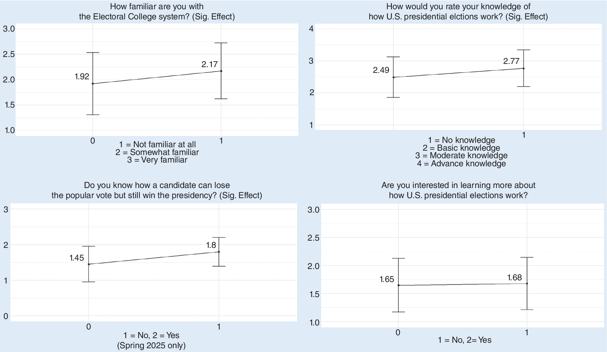
To further examine students’ learning experience, we compared pre- and post-survey responses on self-reported knowledge of US presidential elections, familiarity with the Electoral College, knowledge of election inversions, and interest in learning more about elections. Figures 4 and 5 report the differences in mean responses between the two surveys. On the three self-reported knowledge items, students reported statistically significant gains in the post-survey. Because the surveys were anonymous and not matched at the individual level, these results should be interpreted as descriptive differences between pre- and post-surveys rather than causal estimates of within-student change.Footnote 7 No statistically significant difference was observed for the item that measured interest in learning more.
Student Perceptions of Learning (Pre- and Post-Surveys)

Figure 4 Long description
The figure consists of four line graphs arranged in a two-by-two grid. Each graph plots survey responses on a y-axis against two time points on the x-axis labeled 0 for pre-survey and 1 for post-survey. Each data point includes a mean value and vertical error bars.
Top-left graph: Titled How familiar are you with the Electoral College system? Sig. Effect. The y-axis ranges from 1.0 to 3.0. The scale is 1 equals Not familiar at all, 2 equals Somewhat familiar, and 3 equals Very familiar. The mean increases from 1.92 at point 0 to 2.17 at point 1.
Top-right graph: Titled How would you rate your knowledge of how U.S. presidential elctions work? Sig. Effect. The y-axis ranges from 1 to 4. The scale is 1 equals No knowledge, 2 equals Basic knowledge, 3 equals Moderate knowledge, and 4 equals Advance knowledge. The mean increases from 2.49 at point 0 to 2.77 at point 1.
Bottom-left graph: Titled Do you know how a candidate can lose the popular vote but still win the presidency? Sig. Effect. The y-axis ranges from 0 to 3. The scale is 1 equals No, 2 equals Yes. The mean increases from 1.45 at point 0 to 1.8 at point 1. A note specifies Spring 2025 only.
Bottom-right graph: Titled Are you interested in learning more about how U.S. presidential elections work? The y-axis ranges from 1.0 to 3.0. The scale is 1 equals No, 2 equals Yes. The mean shows a negligible change from 1.65 at point 0 to 1.68 at point 1.
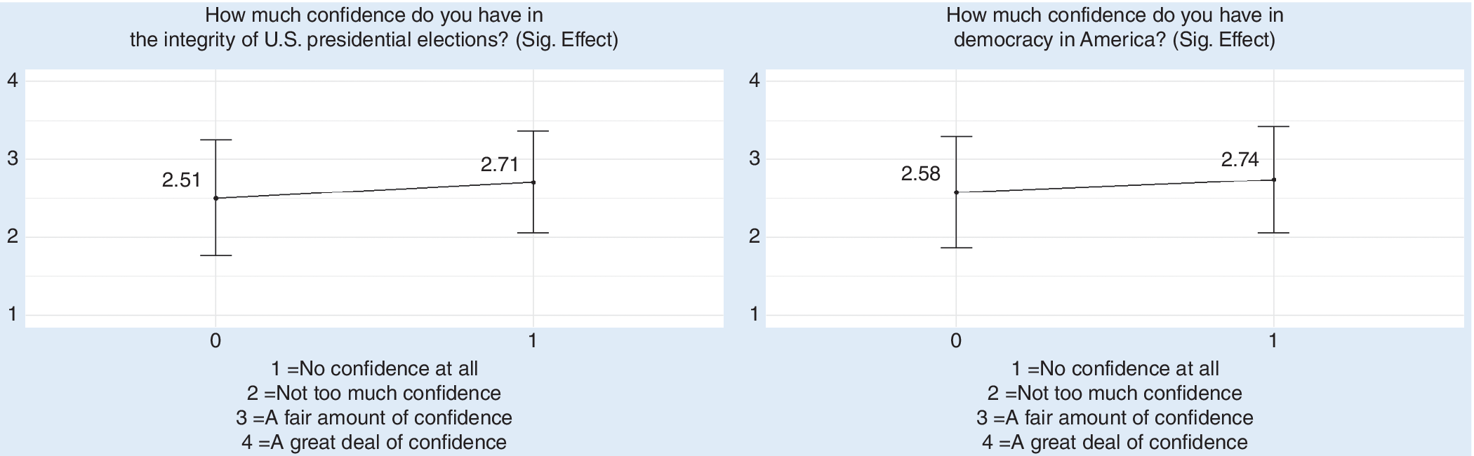
Student Confidence in Election and Democracy (Pre- and Post-Surveys)

Figure 5 Long description
A two-panel figure. Both panels use a y-axis scale from 1 to 4, where 1 equals No confidence at all, 2 equals Not too much confidence, 3 equals A fair amount of confidence, and 4 equals A great deal of confidence. The x-axis represents time with 0 as pre-survey and 1 as post-survey.
Left Panel: Titled How much confidence do you have in the integrity of U. S. presidential elections? (Sig. Effect). A line connects two points. The pre-survey point is at 2.51 with error bars extending from approximately 1.8 to 3.2. The post-survey point is at 2.71 with error bars extending from approximately 2.1 to 3.4.
Right Panel: Titled How much confidence do you have in democracy in America? (Sig. Effect). A line connects two points. The pre-survey point is at 2.58 with error bars extending from approximately 1.9 to 3.3. The post-survey point is at 2.74 with error bars extending from approximately 2.1 to 3.4.
Because election inversions often are viewed as unfair, we were uncertain whether learning about them would increase or decrease students’ confidence in election integrity and democracy. We found a positive and statistically significant difference in the post-survey (see figure 5), in which students reported greater confidence in both the integrity of US presidential elections and democracy in America. Although effect sizes were modest, the direction of the differences was encouraging and consistent with research that has found that voter education can increase political trust. From conversations with students, we learned that completing the exercises helped them better understand election inversions as plausible outcomes of the Electoral College system. Rather than attributing election inversions to alleged voter fraud or other election irregularities, students learned to recognize them as a consequence that naturally arises from the electoral rules.
PEDAGOGICAL CONSIDERATIONS
Based on the instructor’s classroom experiences and students’ feedback, we suggest the following three steps for incorporating the two models into an existing course:
Step 1: Introduce model 1 and table 2 from this article during lecture (10 to 15 minutes). If an instructor is pressed for time, covering these two components alone is sufficient to give students a basic understanding of election inversions without using the worksheets.
Step 2 (optional): Assign students to complete worksheet 1 in class (15 to 20 minutes). The core components of worksheet 1 are the first table and questions 1 and 2, which show how a candidate can win the popular vote but lose the Electoral College vote. Questions 3 through 5 are follow‑up questions that explore additional insights, such as why eliminating the plus-two rule alone would not eliminate election inversions in the Electoral College. If time permits, we recommend that instructors discuss the follow-up questions with students during class to reinforce their understanding.
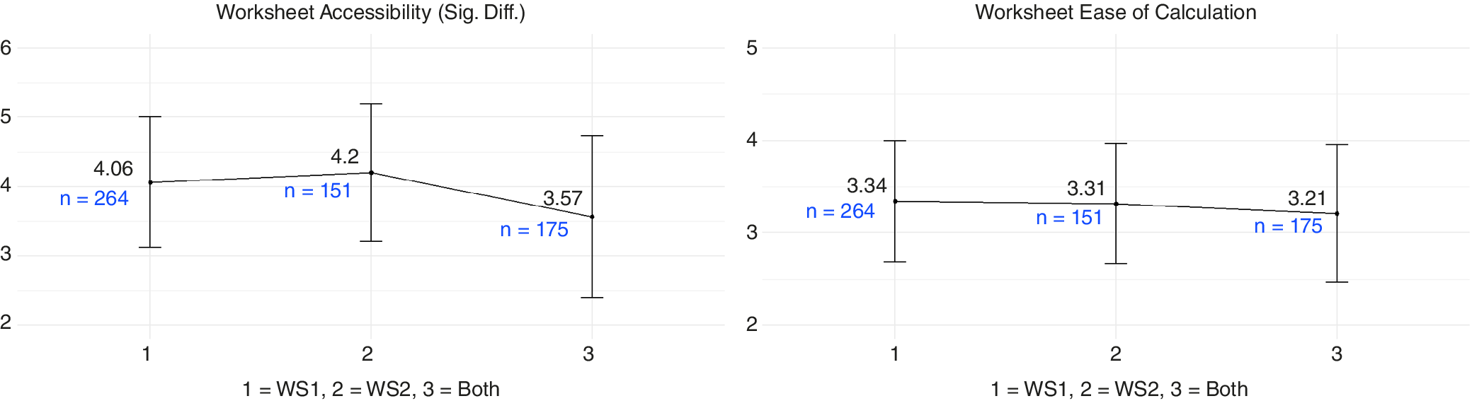
Step 3 (optional): Assign worksheet 2 as homework or include it in an exam. As in worksheet 1, the core material in worksheet 2 is the first table with questions 1 and 2; subsequent follow-up questions explore additional insights. We do not recommend requiring students to complete both worksheets during class time. In the student learning-experience study, students were given only worksheet 1, only worksheet 2, or both worksheets, depending on the course section. As shown in figure 6, completing both worksheets during class reduced perceived accessibility, although it did not increase perceived difficulty. Worksheet 2, therefore, is best used separately.
Figure 6In Class, One Worksheet Is Better Than Two

Figure 6 Long description
A two-panel figure. Both graphs share a common x-axis with three categories: 1 equals W S 1, 2 equals W S 2, and 3 equals Both.
Left Panel: Titled Worksheet Accessibility (Sig. Diff.). The y-axis ranges from 2 to 6.
* At category 1, the mean is 4.06 with n equals 264 and a vertical error bar extending from approximately 3.2 to 5.0.
* At category 2, the mean increases to 4.2 with n equals 151 and an error bar from 3.3 to 5.2.
* At category 3, the mean drops to 3.57 with n equals 175 and a wider error bar from 2.4 to 4.6.
Right Panel: Titled Worksheet Ease of Calculation. The y-axis ranges from 2 to 5.
* At category 1, the mean is 3.34 with n equals 264 and an error bar from 2.7 to 4.0.
* At category 2, the mean is 3.31 with n equals 151 and an error bar from 2.7 to 4.0.
* At category 3, the mean is 3.21 with n equals 175 and an error bar from 2.5 to 3.9.
The data shows a slight downward trend in ease of calculation across the three categories, while accessibility peaks at W S 2.

It is possible to explain an election inversion using only step 1, which can take as few as 10 minutes. However, if time permits, we recommend providing students with the worksheets as an active-learning tool to promote deeper understanding.
ADDITIONAL FACTORS CONTRIBUTING TO ELECTION INVERSIONS
Although the two models presented in this article focus on the effects of the House-seats-plus-two rule and the winner-take-all system, they are not the only factors that contribute to election inversions. The social choice literature that examines the Electoral College as a two-stage voting system identifies additional structural and electoral factors. First, House size matters: the number of House seats has been capped at 435 since 1929 despite continuous population growth and increasing population disparities across states. Consequently, House apportionment has become “coarser” over time with an increase in rounding errors (Ladewig and Jasinski Reference Ladewig and Jasinski2008). For example, following the 2020 US Census, Montana had two House seats with an average district size of 542,113, and Delaware had one at-large seat with an average district size of 989,948. This increasing degree of imbalance alone could contribute to election inversions (Geruso, Spears, and Talesara Reference Geruso, Spears and Talesara2022; Miller Reference Miller2014). Simulations demonstrate that by increasing the size of the House to allow for better proportionality, the probability of inversions in the Electoral College can be reduced significantly (Barthélémy, Martin, and Piggins Reference Barthélémy, Martin and Piggins2014; Neubauer and Zeitlin Reference Neubauer and Zeitlin2003).
Among the electoral factors influencing the probability of inversions, a significant one is the closeness of an election (Merrill Reference Merrill1978). Ball and Leuthold (Reference Ball and Leuthold1991) showed that when the vote margin between the two major-party candidates is 1% or less, the probability of an inversion is at least 30%. Geruso, Spears, and Talesara (Reference Geruso, Spears and Talesara2022, 327) updated the probability to approximately 40%: “…the United States has experienced so few inversions merely because there have been so few elections (and fewer close elections).” A second electoral factor is the uneven voter-turnout rates across states, which further reduces the representativeness of a state’s Electoral College votes (Geruso, Spears, and Talesara Reference Geruso, Spears and Talesara2022; Miller Reference Miller, Felsenthal and Machover2012). House apportionment is based on each state’s total resident population, which includes both citizens and noncitizens. Some citizens are eligible to vote and others are not, such as minors and disenfranchised individuals. Among eligible voters, only approximately 60% cast ballots in a given presidential election in recent decades, and turnout rates vary significantly across states. Consequently, although the number of Electoral College votes allocated to a state is determined by its resident population, how those votes are cast is determined by only a fraction of that population: eligible citizens who actually vote. For example, in the 2020 US presidential election, the lowest turnout-to-resident-population state was Texas at 38.7%; within that percentage, 50.06% voted for Trump. In other words, a mere
$ 38.7\%\times 50.06\%=20.15\% $
 of Texas’s total resident population delivered 38 Electoral College votes to Trump, despite the fact that 36 of those votes were apportioned on the basis of the state’s total resident population.
The potential for election inversions in the Electoral College has long been recognized in the literature, with many scholars viewing them as problematic and a reason for electoral reform (Dahl Reference Dahl2003; Edwards Reference Edwards2023; Fon Reference Fon2004). Because the winner-take-all system and the House-seats-plus-two rule are not the only factors contributing to election inversions, even if they were removed through reform, the frequency of election inversions might be reduced but not entirely eliminated (Cervas and Grofman Reference Cervas and Grofman2019; Fon Reference Fon2004; Miller Reference Miller, Felsenthal and Machover2012). In worksheet 1, question 4 illustrates this exact point with an example. “The outcome of the electoral vote in a state, and hence the outcome of the Electoral College vote, depends on the margin of victory but not on voter-participation rates in that state. The outcome of the nationwide popular vote depends on voter participation in every state but not on the margin of victory in each state.” As long as the Electoral College remains a two-stage voting system, “…there can be no expectation that the popular-vote winner will necessarily win the Presidency” (Fon Reference Fon2004, 67–68).
A key insight in the study of elections as preference aggregation systems is that election rules—not only votes—directly shape electoral outcomes. Some rules (e.g., voter ID laws) have an obvious effect on election outcomes because they influence voter turnout and therefore the votes that are cast. However, even election rules that do not affect voters directly—that is, the vote-tallying rules that seem to be purely mathematical and mechanical—also can determine who wins and who loses an election. The Electoral College is one such example, as well as Ranked Choice Voting—an alternative voting method that recently has been garnering more attention in election reforms. The fact is that if the votes remain constant but the vote-tallying rules change, it is possible that different rules will produce different outcomes. (For readers who are interested in exploring this topic further, a list of introductory books is in the online appendix.)
A key insight in the study of elections as preference aggregation systems is that election rules—not only votes—directly shape electoral outcomes.
CONCLUDING REMARKS
The two models presented in this article are designed as teaching tools for election inversions in undergraduate political science courses such as Introduction to American Politics, Campaigns and Elections, Voting Behavior, and Political Participation. They require neither specialized training on the part of the instructor nor advanced mathematical skills on the part of the students. Model 1 and table 2 can be explained in as few as 10 minutes during a lecture. The worksheets can be used in a large lecture class, in smaller breakout sessions, as homework assignments, and as exam questions. By developing a basic understanding of the mathematical foundations of election methods, students will be better equipped to engage in informed and meaningful discussions about voting and elections, and they may even gain greater confidence in the integrity of elections and democracy. We encourage instructors to adopt these models in their courses because these relatively minor additions can result in meaningful gains in student learning.
By developing a basic understanding of the mathematical foundations of election methods, students will be better equipped to engage in informed and meaningful discussions about voting and elections, and they even may gain greater confidence in the integrity of elections and democracy.
SUPPLEMENTARY MATERIAL
To view supplementary material for this article, please visit http://doi.org/10.1017/S1049096526102339.
DATA AVAILABILITY STATEMENT
Research documentation and data that support the findings of this study are openly available at the PS: Political Science & Politics Harvard Dataverse at https://doi.org/10.7910/DVN/GYHFCX.
CONFLICTS OF INTEREST
The authors declare that there are no ethical issues or conflicts of interest in this research.