2. Problem formulation

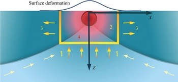
A liquid layer with a line heat source located at the surface is considered (figure 1). The coordinate system $XZ$ has the origin at the heat source location, the vertical axis $Z$ is directed downwards. Similar to an impinging jet, three flow regions can be identified: a stagnation region near the heat source, a boundary layer which is formed along the surface and the entrained flow region located below the boundary layer.

Figure 1.

Flow configuration: $1$ – entrained flow region, $2$ – stagnation region, $3$ – boundary layer, $4$ – line heat source.

The flow is described by two-dimensional (2-D) Navier–Stokes equations in the Boussinesq approximation

(2.1)$$\begin{gather} \displaystyle\frac{\partial V_i}{\partial X_i}=0, \end{gather}$$

(2.2)$$\begin{gather}\displaystyle\rho\left(\frac{\partial V_i}{\partial \tilde{t}}+V_j\frac{\partial V_i}{\partial X_j}\right) ={-}\frac{\partial P}{\partial X_i}+\frac{\partial}{\partial X_j}\left[\eta \left(\frac{\partial V_i}{\partial X_j}+\frac{\partial V_j}{\partial X_i} \right) \right]+\rho g_i, \end{gather}$$

(2.3)$$\begin{gather}\displaystyle \rho c_p \left( \frac{\partial\theta}{\partial\tilde{t}}+V_i\frac{\partial\theta}{\partial X_i} \right)=\frac{\partial}{\partial X_i}\left(\lambda \frac{\partial \theta}{\partial X_i} \right). \end{gather}$$

Here $\rho$, $P$, $\theta$ and $V_{1,2}$ denote, respectively, density, pressure, temperature and the velocity components, $X_{1,2}$ are the vertical and horizontal coordinates, $\tilde {t}$ is time, $\eta$, $\lambda$ and $c_p$ are, respectively, dynamic viscosity, thermal conductivity and specific heat of the liquid, $g$ is the acceleration of gravity. Initially the liquid is at rest and has uniform temperature $20\,^{\circ }\mbox {C}$. In numerical simulations to be compared with experimental results temperature dependences of $\rho$, $c_p$, $\lambda$, $\eta$ are taken into account using the empirical correlations given in Vinnichenko et al. (Reference Vinnichenko, Pushtaev, Plaksina, Rudenko and Uvarov2018b). A no-slip boundary condition is imposed at all the boundaries, including the liquid surface, which corresponds to the influence of the surface film. The heat source located at the surface is simulated using the constant heat flux specified at the liquid surface for $|X| \leqslant 0.7$ mm. Preliminary simulations, performed with different values of the heated region width, demonstrate that the far-field flow behaviour remains the same. However, the peak temperature value depends strongly on the heated region width. Hence, the width of the heated region is determined by the comparison of the simulation results with IR thermography data. The rest of the liquid surface and the side walls are assumed adiabatic, whereas the bottom wall is isothermal. This corresponds to unsteady flow development after the heating is initiated. For comparison with the proposed similarity solution, which is constructed for a laterally unbounded liquid layer, simulations are also performed for the liquid with constant properties and with free boundaries specified instead of the side walls,

(2.4)\begin{equation} \displaystyle \frac{\partial V_X}{\partial X}=\frac{\partial V_Z}{\partial X}=\frac{\partial \theta}{\partial X}=0. \end{equation}

The surface deformation is described by

(2.5)\begin{equation} p_{air}-p+\rho gh-\sigma\frac{\partial^{2} h}{\partial X^{2}}+2\eta\frac{\partial V_Z}{\partial Z}=0, \end{equation}

where $\sigma$ is the surface tension and $p_{air}$ is atmospheric pressure. Equation (2.5) is solved with respect to the surface elevation $h$. Boundary condition $h=0$ is imposed at the side boundaries, since the moon-glade background oriented Schlieren (MG BOS) technique, employed in experiments, is sensitive to the slope of the liquid surface and does not measure variations of the mean liquid level. The observed liquid surface deformation is small compared with the liquid layer depth $H$ and its influence upon the velocity field can be neglected, since the Galileo number $Ga=gH^{3}/(\nu \chi )$, where $\nu$ is kinematic viscosity and $\chi$ is thermal diffusivity, is large and the crispation number $Cr=\eta \chi /(\sigma H)$ is small (Nepomnyashchy, Velarde & Colinet Reference Nepomnyashchy, Velarde and Colinet2001).

3. Similarity solution

The similarity solution is constructed for a 2-D laminar boundary layer in a laterally unbounded domain. Temporal dependencies of the horizontal and vertical length scales of the transient flow were derived by Mori & Niino (Reference Mori and Niino2002) for horizontal convection driven by a sudden decrease of temperature at half of the bottom wall. In contrast, a steady state of the flow within a finite measurement region around the heat source is assumed in the present study. In experiments this corresponds to a time period, when the unsteady perturbations have already left the measurement region in the central part of the tank, but the heat losses to the environment can still be neglected.

Boundary layer equations are written in dimensionless form

(3.1)\begin{equation} \left. \begin{gathered} \displaystyle \frac{\partial v_x}{\partial x}+\frac{\partial v_z}{\partial z}=0,\\ \displaystyle \frac{1}{Pr}\left( v_x\frac{\partial v_x}{\partial x}+v_z\frac{\partial v_x}{\partial z} \right)={-}\frac{\partial p}{\partial x}+\frac{\partial^{2} v_x}{\partial z^{2}}, \\ \displaystyle 0={-}\frac{\partial p}{\partial z}-RaT, \\ \displaystyle v_x\frac{\partial T}{\partial x}+v_z\frac{\partial T}{\partial z} = \frac{\partial^{2} T}{\partial z^{2}}. \end{gathered}\right\} \end{equation}

Spatial coordinates, time, the velocity components, pressure and temperature perturbations are made dimensionless with $l$, $l^{2}/\chi$, $\chi /l$, $\eta \chi /l^{2}$ and $q/\lambda$, respectively. Here $q$ is the heating power per unit length, $l$ is the characteristic length, which will be defined below; $Pr=\eta c_p/\lambda$ is the Prandtl number and $Ra={\rho g \beta q l^{3}}/{\eta \chi \lambda }$ is the Rayleigh number, $\beta$ is the thermal expansion coefficient. Liquid properties, except for density, are assumed constant. Note that the $z$-momentum equation, which contains the transverse pressure gradient related to buoyancy, is not omitted. Pressure is eliminated by subtracting the $z$-momentum equation, differentiated with respect to $x$, from the $x$-momentum equation, differentiated with respect to $z$,

(3.2)\begin{equation} \frac{1}{Pr} \frac{\partial}{\partial z} \left( v_x \frac{\partial v_x}{\partial x}+v_z\frac{\partial v_x}{\partial z} \right)-\frac{\partial^{3}}{\partial z^{3}}v_x=Ra\frac{\partial T}{\partial x}. \end{equation}

To satisfy the continuity equation, the streamfunction $\psi (x,z)$ is introduced,

(3.3a,b)\begin{equation} v_x=\frac{\partial \psi}{\partial z},\quad v_z={-}\frac{\partial \psi}{\partial x}, \end{equation}

and the similarity solution is sought in the form

(3.4a,b)\begin{equation} \psi(x, z)=x^{a}f(z^{b} x^{c}), \quad T(x,z)=x^{d}\phi(z^{b} x^{c}). \end{equation}

Equations (3.4a,b) are substituted into (3.2) and into the energy equation from (3.1). Taking into account the boundary conditions at the surface and the fact that the energy convected across any vertical plane in the boundary layer does not depend on $x$, the exponents in (3.4a,b) are uniquely determined as

(3.5a–d)\begin{equation} a=1/2, \quad b=1, \quad c ={-}1/2, \quad d={-}1/2. \end{equation}

Since the problem formulation does not contain any specific spatial scale, it is convenient to define the characteristic length $l$ so that $Ra = 1$, that is,

(3.6)\begin{equation} l=\sqrt[3]{\frac{\eta\chi\lambda}{\rho g \beta q}}. \end{equation}

Then $Pr$ becomes the only parameter remaining in (3.1). Similarity solutions, obtained for the temperature and velocity distributions, are

(3.7)\begin{equation} \left.\begin{gathered} \displaystyle T(x,z) = \frac{\phi(\xi)}{\sqrt{x}}, \\ \displaystyle v_x(x,z)=f'(\xi), \\ \displaystyle v_z(x, z)=\frac{f'(\xi)\xi-f(\xi)}{2\sqrt{x}}, \end{gathered}\right\} \end{equation}

where $\xi ={z}/{\sqrt {x}}$ is the similarity variable. Note that the expressions for the similarity variable and the velocity components are essentially the same as for the laminar boundary layer along a flat plate (Schlichting & Gersten Reference Schlichting and Gersten2017). However, the velocity and temperature fields are coupled.

Ordinary differential equations, obtained for $f(\xi )$ and $\phi (\xi )$,

(3.8)\begin{equation} \left.\begin{gathered} \displaystyle 2\phi''+(f\phi)'=0, \\ \displaystyle \frac{(ff'')'}{Pr}+2f^{(iv)}-\phi-\xi\phi'=0, \end{gathered}\right\} \end{equation}

can be integrated, taking into account the boundary conditions $f(0)=f^{\prime }(0)=\phi ^{\prime }(0)=0$. Integration leads to

(3.9)\begin{equation} \left.\begin{gathered} \displaystyle \phi^{\prime}={-}\frac{f\phi}{2}, \\ \displaystyle f^{\prime\prime\prime}=\frac{\xi\phi}{2}-\frac{ff^{\prime\prime}}{2Pr}-C. \end{gathered}\right\} \end{equation}

The latter equation, substituted into the $x$-momentum equation in (3.1), yields

(3.10)\begin{equation} \displaystyle \frac{\partial p}{\partial x}=\frac{\xi\phi}{2x}-\frac{C}{x}. \end{equation}

Thus, the unknown constant $C$ determines the pressure gradient at the surface. The boundary layer region extends from the liquid surface ($\xi =0$) to the point $\xi =\xi _{max}$, where the horizontal velocity vanishes. Equations (3.9) require two more boundary conditions: $f^{\prime \prime }(0)$ and $\phi (0)$ must be known to solve the Cauchy problem. The solution for unknown $\phi (0)$ can be obtained from the solution for $\phi (0)=1$ using the heat flow normalization procedure similar to that proposed by Gebhart et al. (Reference Gebhart, Pera and Schorr1970) for the convective plume. In the steady state the heat convected across any vertical plane within the boundary layer must be equal to half of the heat produced by the source, i.e. with the adopted normalizations

(3.11)\begin{equation} \int_0^{z_{max}}v_xT\,\mathrm{d} z = \int_0^{\xi_{max}} f^{\prime}\phi \,\mathrm{d} \xi=\tfrac{1}{2}, \end{equation}

where $z_{max}=\xi _{max}\sqrt {x}$.

If the value of this integral, calculated for the solution with $\phi (0)=1$ (denoted as $f_n$, $\phi _n$, $\xi _n$, $C_n$), is $I/2$, then after transformation

(3.12a–d)\begin{equation} \displaystyle f=\frac{f_n}{I^{{1}/{6}}}, \quad \phi=\frac{\phi_n}{I^{{5}/{6}}}, \quad \xi=\xi_nI^{{1}/{6}}, \quad C=\frac{C_n}{I^{{2}/{3}}}. \end{equation}

Here $f(\xi )$ and $\phi (\xi )$ still satisfy the equations (3.9) and the boundary conditions, and the integral (3.11) becomes equal to $1/2$. Thus, two unknown parameters remain: $f^{\prime \prime }(0)$ and the constant $C$. Their values are determined by the shooting method. The required boundary conditions at $\xi =\xi _{max}$ are obtained from consideration of the flow in the part of the stagnation region located below the boundary layer (region 2 in figure 1).

It follows from the $z$-momentum equation in (3.1) that the pressure drop across the boundary layer does not depend on $x$,

(3.13)\begin{equation} \varDelta p_1={-}\int_0^{z_{max}} T \, \mathrm{d} z={-}\int_0^{\xi_{max}}\phi \, \mathrm{d} \xi={\rm const}. \end{equation}

Therefore, the pressure variation along the surface is determined by the pressure drop in stagnation region below the boundary layer. Velocity is small in this region. Hence, as in the boundary layer

(3.14)\begin{equation} \displaystyle \frac{\partial p}{\partial z} ={-}T. \end{equation}

Neglecting the temperature variation along the horizontal line from the flow centreline $x=0$ to the edge of the boundary layer,

(3.15)\begin{equation} T(z)=\frac{\phi(\xi_{max})}{\sqrt{x}}=\frac{\phi(\xi_{max})}{z}\xi_{max}. \end{equation}

Then, the pressure drop below the boundary layer is

(3.16)\begin{equation} \Delta p_2={-}\phi(\xi_{max})\xi_{max}\ln(\xi_{max}\sqrt{x}) \end{equation}

and the pressure gradient at the surface is

(3.17)\begin{equation} \left. \displaystyle \frac{\partial p}{\partial x}\right|_{z=0} ={-}\frac{\phi(\xi_{max})\xi_{max}}{2x}. \end{equation}

From the comparison with (3.10) for $z=0$ ($\xi =0$) the constant $C$ can be found,

(3.18)\begin{equation} C = \frac{\xi_{max}\phi(\xi_{max})}{2}. \end{equation}

The upward flow in the entrained flow region (region 1 in figure 1) and the horizontal flow in the boundary layer (region 3 in figure 1) must be equal,

(3.19)\begin{equation} \displaystyle \int_0^{z_{max}}v_x\,\mathrm{d} z ={-}\int_0^{x} v_z\,\mathrm{d}x. \end{equation}

But

(3.20)\begin{equation} \displaystyle \int_0^{z_{max}}v_x\,\mathrm{d} z=\sqrt{x}\int_0^{\xi_{max}}f^{\prime}\,\mathrm{d} \xi = \sqrt{x}f(\xi_{max}). \end{equation}

Since the horizontal variation of temperature is neglected in the stagnation region,

(3.21)\begin{equation} v_z\frac{\partial T}{\partial z}=\frac{\partial^{2}T}{\partial z^{2}}. \end{equation}

Substituting (3.15) into (3.21), one can obtain the vertical velocity in the stagnation region,

(3.22)\begin{equation} v_z={-}\frac{2}{z}. \end{equation}

Hence,

(3.23)\begin{equation} \int_0^{x} v_z\,\mathrm{d} x={-}\int_0^{x}\frac{2}{z}\,\mathrm{d} x ={-}\frac{2\sqrt{x}}{\xi_{max}}. \end{equation}

Comparison of (3.20) and (3.23) yields the second condition

(3.24)\begin{equation} f(\xi_{max})=\frac{2}{\xi_{max}}. \end{equation}

It is noteworthy that derivation of (3.18) and (3.24) is based on (3.15), which implies that the temperature variation along the horizontal line from the centreline $x=0$ to the edge of the boundary layer can be neglected. This assumption becomes invalid for small values of Prandtl number ($Pr<1$), when the boundary layer becomes more thick. In this case, the parameters $f^{\prime \prime }(0)$ and $C$ can be determined by comparison of the similarity solution with numerical simulation. To solve the Cauchy problem, the fourth-order Runge–Kutta method is used. Here $\xi _{max}$, at which the horizontal velocity $v_x=f^{\prime }$ vanishes, is determined from the solution. For $Pr=7.16$ (water at $20\,^{\circ }\mbox {C}$) and $70$, the parameters $f^{\prime \prime }(0)$ and $C$ are determined by the shooting method using the conditions (3.18) and (3.24). For $Pr=0.1$ and $0.7$, their values are taken from the numerical simulations. The obtained values of the similarity solution parameters are given in table 1.

Table 1.

Parameters of the similarity solution for various Prandtl numbers. Here $\xi _0$ is the location of the dimensionless horizontal velocity maximum $f^{\prime }_{max}$.

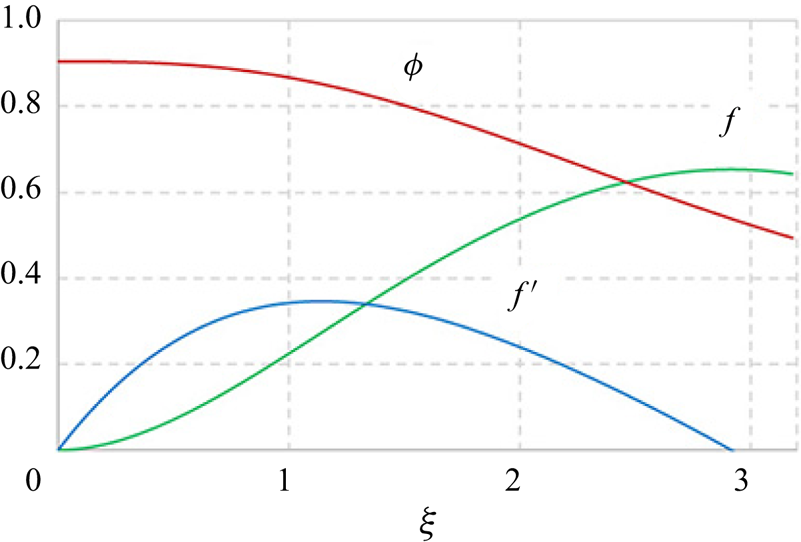
The results for $Pr=7.16$ and $70$ demonstrate that for large Prandtl numbers the influence of the nonlinear term in the second equation (3.9) becomes small and the asymptotic solution is reached. The obtained profiles of $f(\xi )$, $f^{\prime }(\xi )$, and $\phi (\xi )$ for $Pr=7.16$ are shown in figure 2.

Figure 2.

Computed profiles of $f(\xi )$, $f^{\prime }(\xi )$ and $\phi (\xi )$ for $Pr=7.16$.

From the similarity solution, it is also possible to obtain the expressions for the maximal dimensional velocity and the boundary layer thickness $V_{X\ max}(q)$ and $Z_{max}(X,q)$,

(3.25)$$\begin{gather} V_{X \ max}(q)=f^{\prime}_{max}\sqrt[3]{\frac{\rho \chi^{2} g\beta}{\eta\lambda} q}\sim q^{{1}/{3}}, \end{gather}$$

(3.26)$$\begin{gather}Z_{max}(X, q) = \xi_{max}\sqrt{X}\sqrt[6]{\frac{\eta\chi\lambda}{\rho g \beta q}} \sim q^{-{1}/{6}}. \end{gather}$$

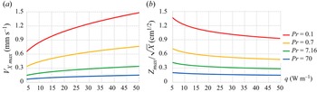
Thus, the maximal velocity is determined by the liquid properties and the heating power. Figure 3 presents the dependencies of $V_{X \ max}$ and $Z_{max}/\sqrt {X}$ on the heating power.

Figure 3.

Plots of (a) $V_{X\ max}$, (b) $Z_{max}/\sqrt {X}$ as functions of the heating power for $Pr=0.1$, $0.7$, $7.16$, $70$.

It is interesting that the same scaling (boundary layer thickness $\sim q^{-1/6}$, velocity $\sim q^{1/3}$) was obtained by Mullarney et al. (Reference Mullarney, Griffiths and Hughes2004) for horizontal convection, driven by differential heating of the bottom wall. For the laterally unbounded domain, the local horizontal Rayleigh number $Ra_X$, based on the distance from the heat source $X$, is defined as

(3.27)\begin{equation} Ra_X=\frac{\rho g \beta q X^{3}}{\eta \chi \lambda}. \end{equation}

However, to compare the results with Mullarney et al. (Reference Mullarney, Griffiths and Hughes2004), who considered horizontal convection in a tank with finite width $L$, $X=L$ is used as a representative value. In our experiments, the horizontal Rayleigh number $Ra_L$, based on the tank width $L=12.3\ \mbox {cm}$, is $1.4\times 10^{9}$ for $q=31\ \textrm {W}\ \textrm {m}^{-1}$ and $2.7\times 10^{9}$ for $q=62\ \textrm {W}\ \textrm {m}^{-1}$, respectively. The thickness of the boundary layer $Z_{max}$ at $X = L$ is denoted by $b$. Thus,

(3.28)\begin{equation} \xi_{max}=\frac{b}{\sqrt{L}}. \end{equation}

Using the vertical profiles of temperature and horizontal velocity, measured experimentally, Mullarney et al. (Reference Mullarney, Griffiths and Hughes2004) obtained

(3.29)\begin{equation} \left.\begin{gathered} \displaystyle \frac{b}{L}=2.649Ra_F^{{-}1/6}, \\ \displaystyle \frac{V_X L}{\chi}=0.45525Ra_F^{1/3}, \end{gathered}\right\} \end{equation}

where $Ra_F$ is the Rayleigh number, based on the heat flux and the tank width. For the similarity solution, constructed in the present study, (3.25), (3.26) yield

(3.30)\begin{equation} \left.\begin{gathered} \displaystyle \frac{b}{\sqrt{L}}=\xi_{max}\sqrt[6]{\frac{\eta\chi\lambda}{\rho g \beta q}}, \quad \mbox{i.e.} \quad \frac{b}{L}=\xi_{max}Ra_L^{{-}1/6}, \\ \displaystyle V_{X\ max}(q)=f^{\prime}_{max}\sqrt[3]{\frac{\chi^{2}g\beta q}{\nu\lambda}},\quad \mbox{i.e.} \quad \frac{V_{X max}L}{\chi}=f^{\prime}_{max}Ra_L^{1/3}. \end{gathered}\right\} \end{equation}

Values of $\xi _{max}$ and $f^{\prime }_{max}$ for various $Pr$ can be found in table 1. For $Pr=7.16$, they are equal to $2.9152$ and $0.3463$, respectively.

4. Nusselt number

Several definitions of Nusselt number can be used to characterize the strength of horizontal convection (Mullarney et al. Reference Mullarney, Griffiths and Hughes2004; Siggers, Kerswell & Balmforth Reference Siggers, Kerswell and Balmforth2004; Rocha et al. Reference Rocha, Bossy, Llewellyn Smith and Young2020a,Reference Rocha, Constantinou, Llewellyn Smith and Youngb). Taking into account the symmetry of the flow and the fact that the heat is transported only within the boundary layer (according to (3.21), the advective and conductive heat fluxes balance each other in the stagnation region), the local Nusselt number at dimensionless distance $r$ from the heat source can be defined as

(4.1)\begin{equation} Nu_{loc}(r)=\frac{\displaystyle q/2}{\lambda\Delta \theta}\frac{\displaystyle {\rm \pi}/2}{\varphi_{max}}= \frac{\rm \pi}{4T\varphi_{max}}, \end{equation}

where $\varphi _{max}$ is the polar angle value, which corresponds to the edge of the boundary layer

(4.2)\begin{equation} \xi_{max}=\frac{z_{max}}{\sqrt{x}}=\sqrt{r}\frac{\sin \varphi_{max}}{\sqrt{\cos \varphi_{max}}}. \end{equation}

For large $r$, the angle is small,

(4.3)\begin{equation} \varphi_{max}=\frac{\xi_{max}}{\sqrt{r}} \end{equation}

and $x\approx r$.

Using the similarity solution (3.7) for temperature perturbation,

(4.4)\begin{equation} Nu_{loc}(r)=\frac{{\rm \pi} r}{4\phi (0) \xi_{max}}. \end{equation}

For the length of the boundary layer $X$,

(4.5)\begin{equation} Nu_{loc}=\frac{{\rm \pi} X}{4\phi (0) \xi_{max}l}=\frac{{\rm \pi} X}{4\phi (0) \xi_{max}}\sqrt[3]{\frac{\rho g \beta q}{\eta\chi\lambda}}=\frac{\rm \pi}{4\phi (0) \xi_{max}}Ra^{1/3}_X\approx 0.3 Ra_X^{1/3}. \end{equation}

Also, the local Nusselt number can be defined, as in Rocha et al. (Reference Rocha, Constantinou, Llewellyn Smith and Young2020b), as the ratio of the heat transported by the convective flow through the surface, located at dimensionless distance $r$ from the heat source, to the heat transported in stagnant liquid. Note that in the present study the power of the heat source is specified, whereas the temperature distribution at the top surface was prescribed in Rocha et al. (Reference Rocha, Constantinou, Llewellyn Smith and Young2020b). Hence, the heat transported in stagnant liquid should be evaluated only within the boundary layer and with the actual temperature distribution, expressed by the similarity solution (3.7). Thus,

(4.6)\begin{equation} \displaystyle Nu_{loc}(r)=\frac{q/2}{\displaystyle \lambda \int_{0}^{\varphi_{max}} (\partial \theta/\partial r)r\,\mathrm{d} \varphi}=\frac{1}{\displaystyle 2\int_{0}^{\varphi_{max}}(\partial T/ \partial r)r\,\mathrm{d} \varphi}. \end{equation}

From the similarity solution,

(4.7)\begin{align} r\frac{\partial T}{\partial r} = r\frac{\partial}{\partial r} \left( \frac{\phi(\xi)}{\sqrt{r\cos \varphi}} \right)=\frac{\phi^{\prime}(\xi (r, \varphi))r\sin \varphi-\phi (\xi (r, \varphi))\sqrt{r}\cos \varphi}{2r(\cos \varphi)^{3/2}}\approx \frac{\phi^{\prime}(\xi)\varphi}{2}-\frac{\phi(\xi)}{2\sqrt{r}}. \end{align}

Numerical integration leads to

(4.8)\begin{equation} Nu_{loc}=A_1 Ra_X^{1/3}, \end{equation}

where $A_1=0.3312$, $0.3165$, $0.3167$, $0.2894$ for $Pr=0.1$, $0.7$, $7.16$, $70$, respectively. For horizontal convection in a tank with width $L$, driven by a prescribed temperature profile at the top wall, Rocha et al. (Reference Rocha, Bossy, Llewellyn Smith and Young2020a) obtained the bound

(4.9)\begin{equation} Nu_{loc} < 0.0525 Ra_L^{1/3}, \end{equation}

which is in qualitative agreement with (4.5) and (4.8). The total Nusselt number can be defined, similar to Mullarney et al. (Reference Mullarney, Griffiths and Hughes2004), as the ratio of the total heat, transported by convective flow, to the heat transported in stagnant liquid with the same temperature distribution,

(4.10)\begin{equation} Nu_{tot}=\frac{\rho c_p V_X b \Delta\theta}{\lambda\Delta\theta}=\frac{V_X b}{\chi}. \end{equation}

Substituting (3.25), (3.26),

(4.11)\begin{equation} Nu_{tot}=f^{\prime}_{max}\xi_{max}\sqrt{\displaystyle \frac{L}{l}}=A_2Ra_L^{1/6}, \end{equation}

where $A_2=0.8234$, $0.8136$, $1.0095$, $0.9234$ for $Pr=0.1$, $0.7$, $7.16$, $70$, respectively. The total Nusselt number $Nu_{tot}=0.81587 Ra_L^{1/6}$ was experimentally obtained by Mullarney et al. (Reference Mullarney, Griffiths and Hughes2004) for horizontal convection in a tank with a non-uniformly heated bottom wall. Thus, despite the different flow configurations, not only the scaling exponents but also the proportionality coefficients appear to be similar, which demonstrates universality of the horizontal convection driven by the horizontal pressure gradient. In § 7 a comparison of the constructed similarity solution with experimental data and the numerical simulation results is performed.

5. Numerical modelling

Equations (2.1)–(2.3) with boundary conditions, described in § 2, are solved numerically using the second-order semi-implicit scheme with the third-order Runge–Kutta method for convective terms and the Crank–Nicolson method for diffusion terms. The fractional-step method is used to find the velocity and pressure corrections in order to satisfy the continuity equation. Spatial discretization involves central differences for diffusion terms and four-points upwind differences for convective ones. Since the free surface deformation is small, a no-slip boundary condition, representing the influence of the surface film, is imposed at the top horizontal boundary, which coincides with the initial position of the deformable free surface. The surface deformation is obtained by solving (2.5) at each time step. Simulations are performed on a staggered grid with the grid step increasing from the heat source to the bottom and side walls of the tank. The same code was used by Vinnichenko et al. (Reference Vinnichenko, Uvarov and Plaksina2014) and by Vinnichenko et al. (Reference Vinnichenko, Pushtaev, Plaksina, Rudenko and Uvarov2018b) for simulations of similar flows: convective plume from a horizontal heated wire and horizontal convection driven by non-uniform radiative heating of the liquid free surface. In Vinnichenko et al. (Reference Vinnichenko, Pushtaev, Plaksina, Rudenko and Uvarov2018b) verification of the code was performed for a related problem – convection of fluid with $Pr=1000$ in a rectangular cavity with no-slip walls and a sinusoidal temperature profile, prescribed at the top boundary, which was considered by Pigeonneau & Flesselles (Reference Pigeonneau and Flesselles2012). According to the results of these earlier studies and the grid convergence study, which involved simulations using three different meshes with minimal grid step $49$, $37$ and $25\ \mathrm {\mu }\textrm {m}$, $100 \times 100$ grid with minimal grid step $25\ \mathrm {\mu }\textrm {m}$ is chosen for simulations. Computational domain size $123 \times 25$ mm corresponds to the tank width and liquid layer depth in the performed experiments. Simulations for verification of the proposed similarity solution are performed using a larger domain $246 \times 50$ mm with boundary conditions (2.4) instead of the side walls. Additional simulations are performed to investigate the influence of the tank width on the flow structure. These results are presented in the supplementary material available at https://doi.org/10.1017/jfm.2022.502.

6. Experimental techniques and procedure

Experiments are performed in a rectangular glass tank with internal dimensions $123\times 132 \times 65$ mm filled with distilled water to the depth $25$ mm. Copel wire with diameter $0.2$ mm is installed horizontally at the liquid surface parallel to the longest side of the tank and heated with $q=31\ \textrm {W}\ \textrm {m}^{-1}$. Experiments are performed at room temperature about $20\,^{\circ }\mbox {C}$ with relative humidity about 40 %. Three experimental techniques are used in separate experimental runs for measurements of the velocity, surface temperature and surface relief instantaneous fields: particle image velocimetry (PIV), IR thermography and MG BOS. Note that the latter technique, which yields surface relief maps, enables one to estimate pressure distribution at the surface using (2.5). Infrared thermography and MG BOS also provide monitoring of the flow uniformity in a direction parallel to the wire. In order to suppress convection driven by evaporation, the tank is covered either with a glass sheet (for PIV and MG BOS) or with a $6$ mm ZnSe plate (for IR thermography), which has a transmittance of about $0.6$ in the wavelength range $1{-}15\ \mathrm {\mu }\textrm {m}$. There is an air gap about 2 cm between the cover and water surface.

6.3. Moon-glade background oriented Schlieren

Surface relief maps are obtained using the MG BOS technique, recently proposed by Vinnichenko et al. (Reference Vinnichenko, Pushtaev, Plaksina and Uvarov2020). A schematic of this technique is presented in figure 4. The camera, installed above the liquid surface, images the reflection of the background pattern (black dots, randomly distributed on a transparent film), backlit with an LED panel. Comparison of the reference image, taken for an undisturbed liquid surface, with the distorted images taken during the flow development is performed using cross-correlation interrogation. The apparent displacement of the background pattern features is proportional to the local slope of the surface. Instantaneous maps of the surface relief perturbation are obtained from the fields of its first spatial derivatives by solving the Poisson equation. The liquid surface is assumed unperturbed far from the heated wire. Images are acquired at 25 f.p.s. with a Canon EOS 700D DSLR camera and Canon EF $100$ mm $f/2.8$ lens. The glass cover of the tank is inclined to avoid imaging of the background pattern reflection from the glass. The background-to-surface distance, which determines the sensitivity of MG BOS, is $156$ cm. The incidence angle is $8^{\circ }$. Keystone distortion is corrected using the calibration image of a rectangular target, the corners of which determine the coefficients of the projective transform. Images are processed with the same multi-pass direct cross-correlation interrogation used for PIV. Two interrogation passes are performed with interrogation windows $32\times 32$ and $16\times 16$ with $50\,\%$ overlap at the final pass. Heating results in formation of a crest at the heat source location. Its height grows to about $5\ \mathrm {\mu }\textrm {m}$ both in MG BOS measurements and numerical simulations.

Figure 4.

Principle of the surface deformation measurement using MG BOS.

From the surface relief maps, averaged in the direction parallel to the heated wire, surface pressure distribution can be estimated using (2.5). Numerical simulations show that the vertical velocity gradient is negligible and the surface curvature is important only near the heat source. In fact, the surface tension contribution to (2.5) is less than 1 % of the pressure perturbation for $|X|>2.3$ mm. Thus, in the far field the surface tension and vertical velocity gradient contributions both can be neglected and the surface elevation profile, measured with MG BOS, can be converted into the surface pressure profile, which is compared with both the numerical simulation and similarity solution (3.10).