PART ONE
Motivation and background
1 Introduction
We aim to address the question of convergence, under mesh refinement, of numerical approximations for a large class of non-linear partial differential equations. We begin with a representative example by considering the compressible Euler equations, which describe the motion of an inviscid, compressible flow, whose study is of fundamental importance in aerodynamics, astrophysics, climate science and more (Dafermos Reference Dafermos2010). The compressible Euler equations form the following system of non-linear partial differential equations (PDEs):
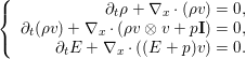 $$\begin{eqnarray}\left\{\begin{array}{@{}r@{}}\partial _{t}{\it\rho}+{\rm\nabla}_{x}\cdot ({\it\rho}v)=0,\\ \partial _{t}({\it\rho}v)+{\rm\nabla}_{x}\cdot ({\it\rho}v\otimes v+p\mathbf{I})=0,\\ \partial _{t}E+{\rm\nabla}_{x}\cdot ((E+p)v)=0.\end{array}\right.\end{eqnarray}$$
Here,  ${\it\rho}$ is the density of the flow,
 $v\in \mathbb{R}^{d}$ (
 $d=1,2,3$) is the velocity vector,
 $p$ is the pressure,
 $E$ denotes the total energy and
 $\mathbf{I}\in \mathbb{R}^{d\times d}$ is the identity matrix. The equation is closed by specifying an algebraic equation of state that relates the thermodynamic variables,
 $p,{\it\rho}$ and
 $E$.
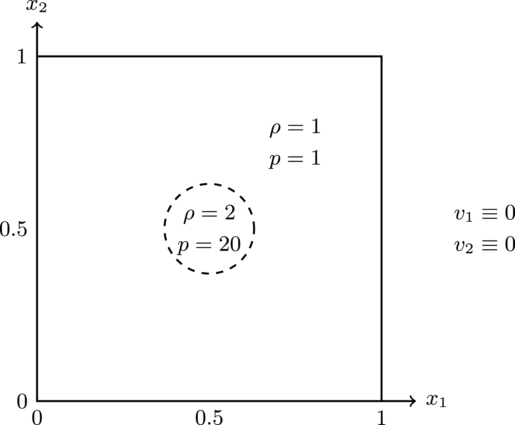
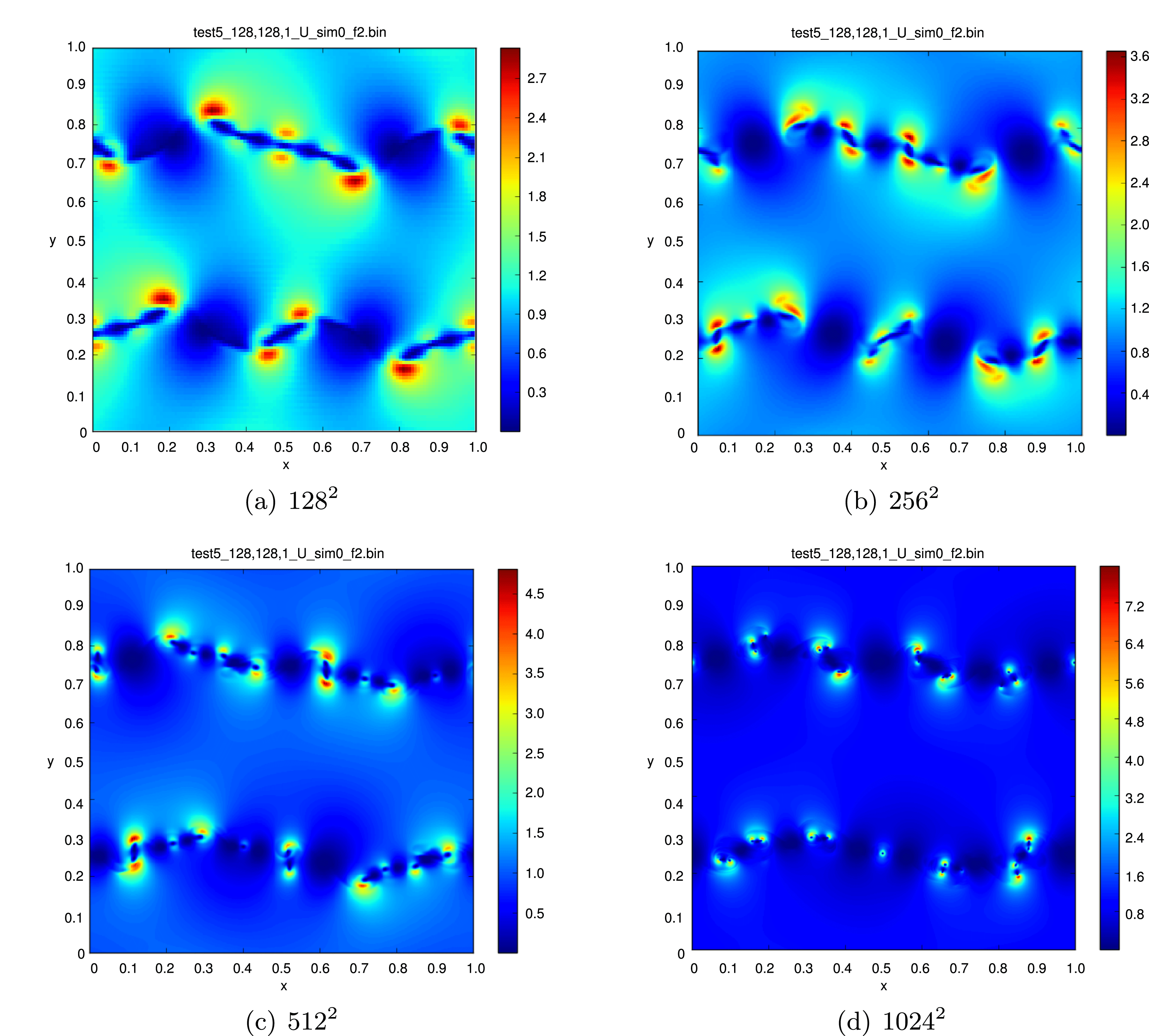
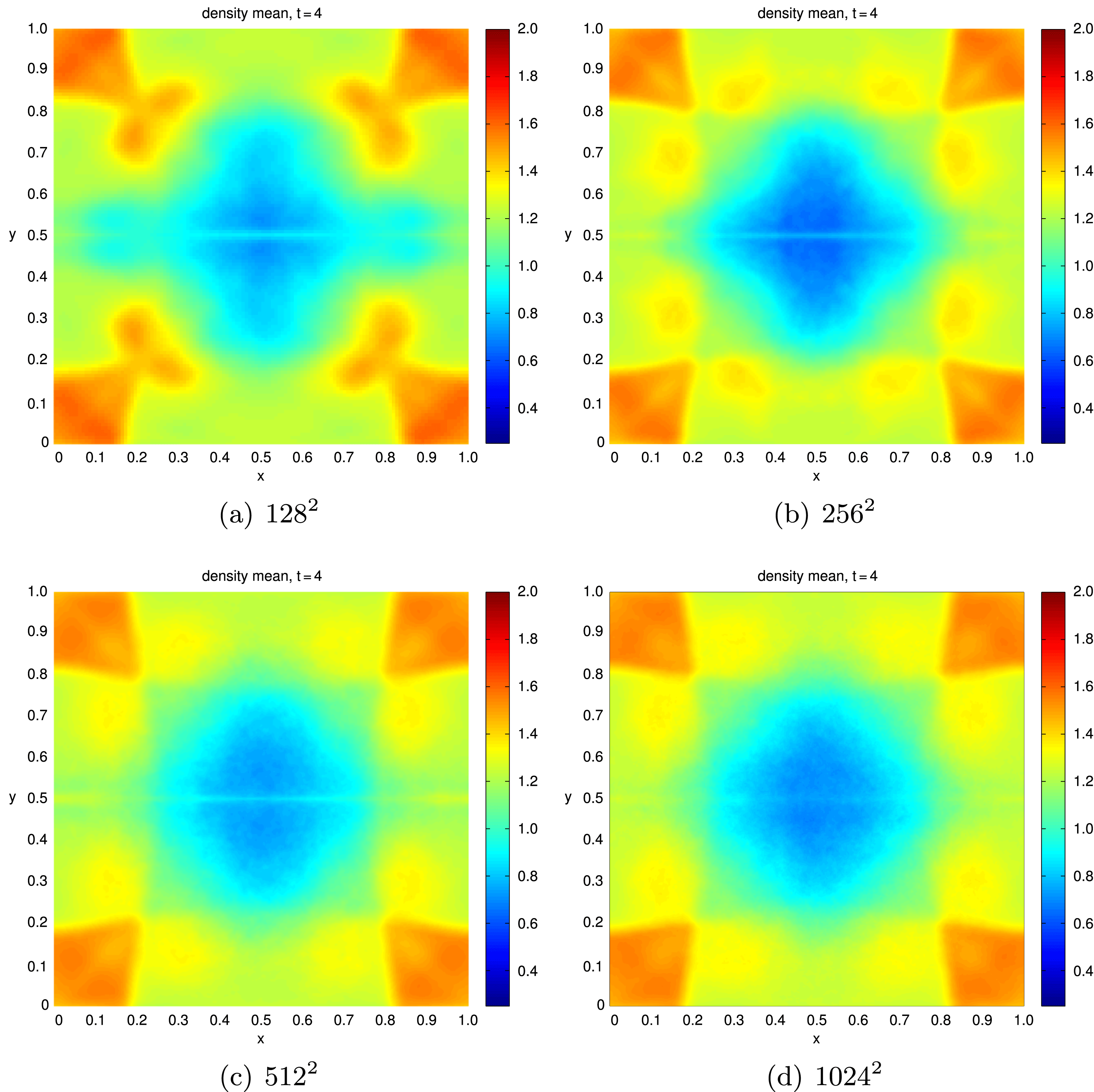
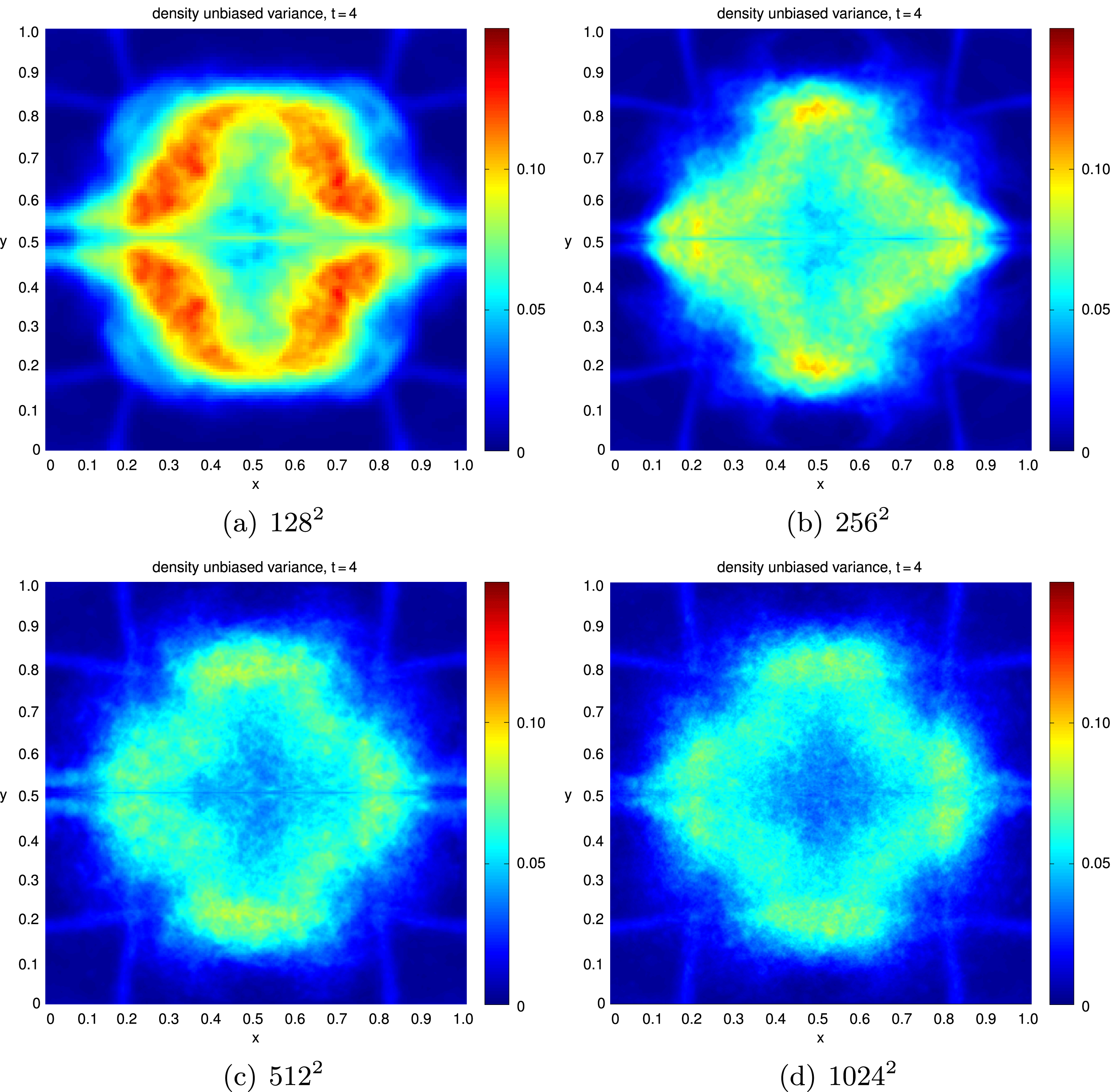
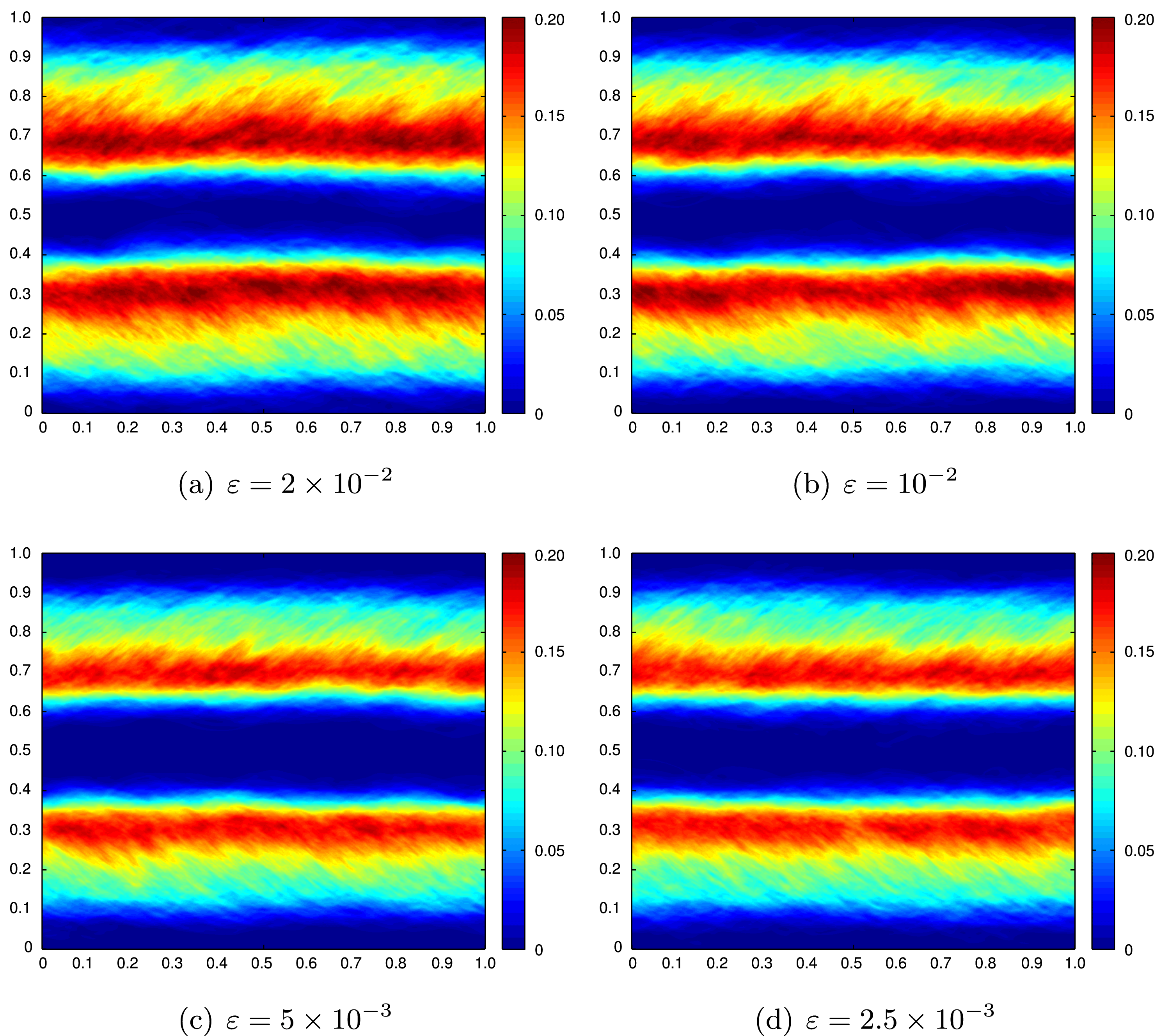
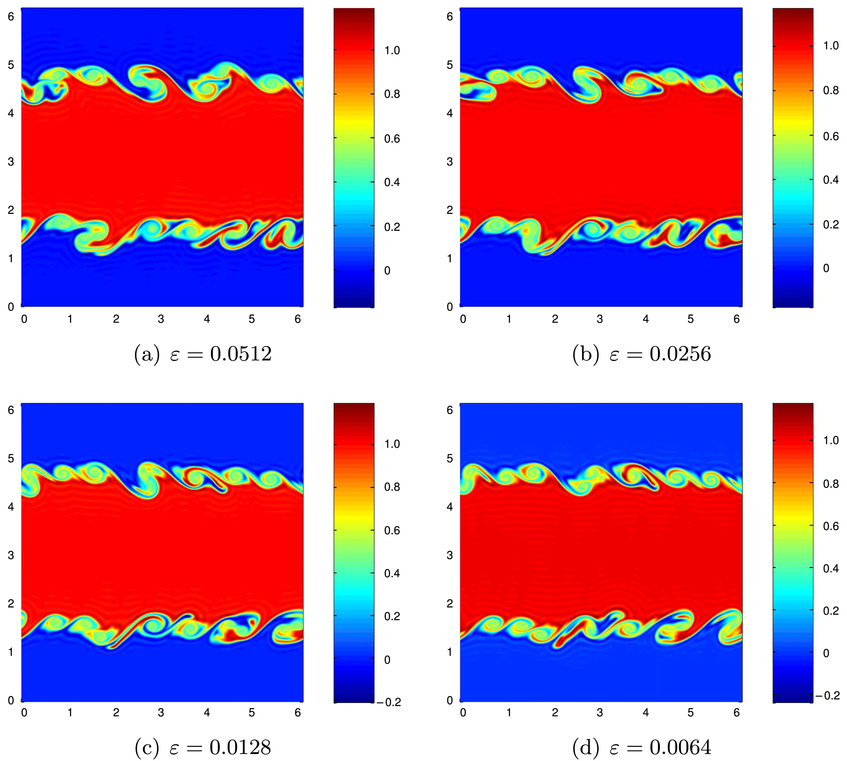
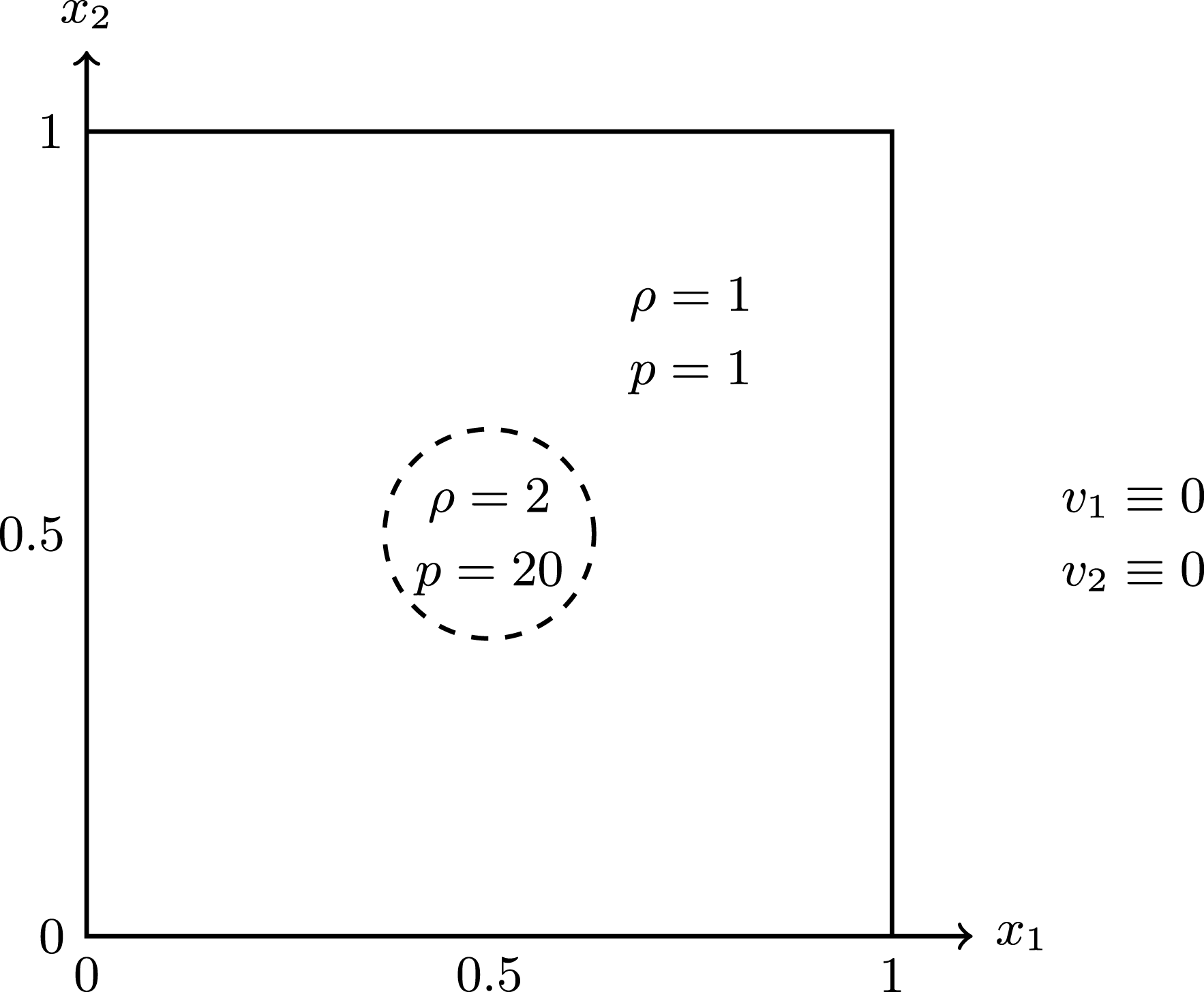
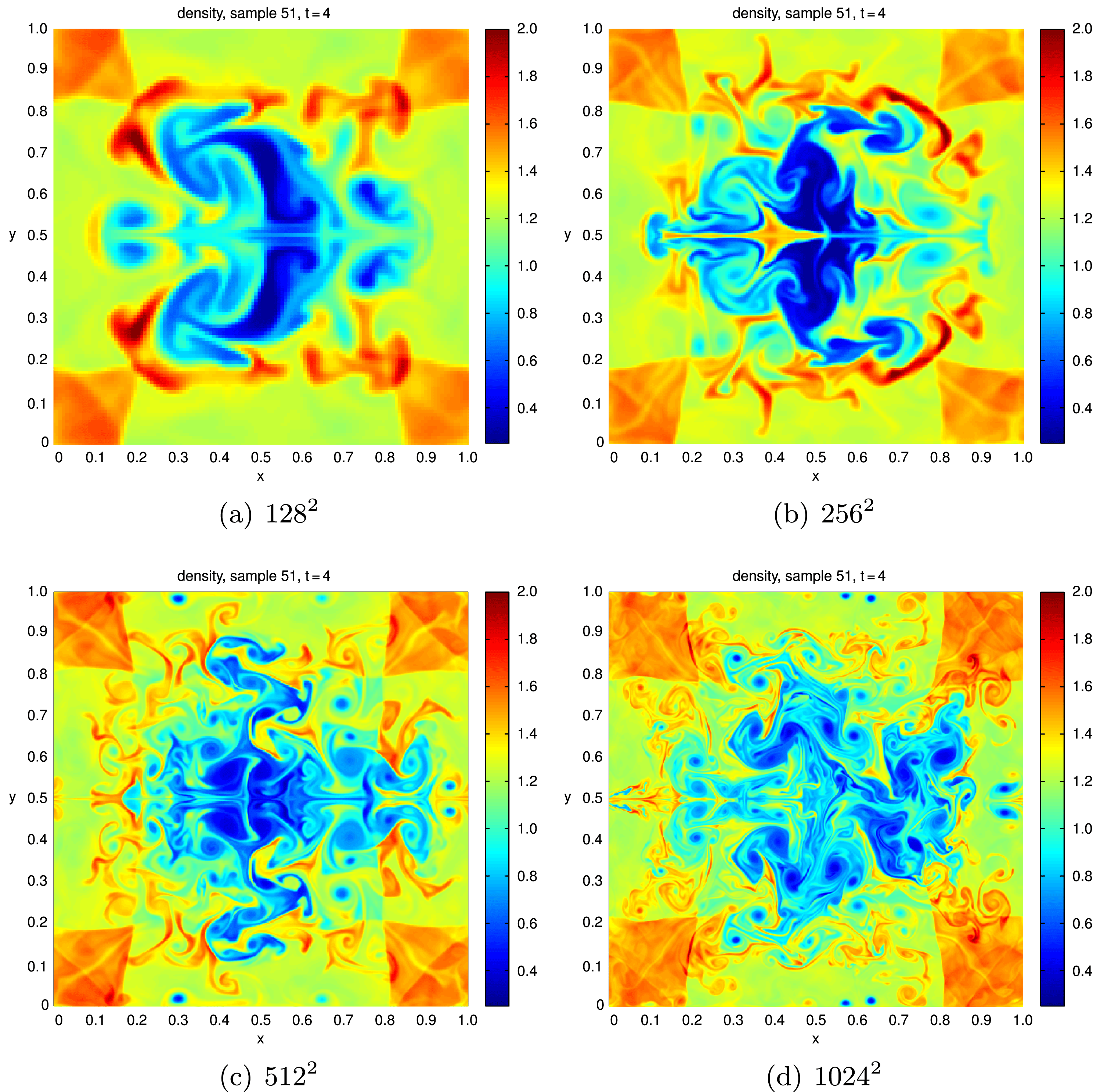
In order to motivate the central issue addressed in this paper, we consider a numerical experiment involving a prototypical state-of-the-art and widely used numerical method for approximating the compressible Euler equations (1.1). This numerical scheme is a high-resolution finite volume scheme, based on an approximate Riemann solver of the HLLC type, a non-oscillatory monotonized-central limiter-based piecewise linear reconstruction, in combination with a second-order, strong stability-preserving Runge–Kutta time-stepping routine. It is implemented within a massively parallel astrophysics code (Käppeli et al. Reference Käppeli, Whitehouse, Scheidegger, Pen and Liebendörfer2011). This scheme is used to discretize the compressible Euler equations (1.1) in the two-dimensional domain  $x\in [0,1]^{2}$ with periodic boundary conditions and with initial conditions shown in Figure 1.1. The initial data are known as the Richtmyer–Meshkov problem (Landau and Lipschitz Reference Landau and Lipschitz1987) and consist of an initial (large) jump in the density and pressure across a slightly perturbed interface. We compute at different mesh resolutions ranging from
 $128^{2}$ to
 $1024^{2}$. The computed density at time
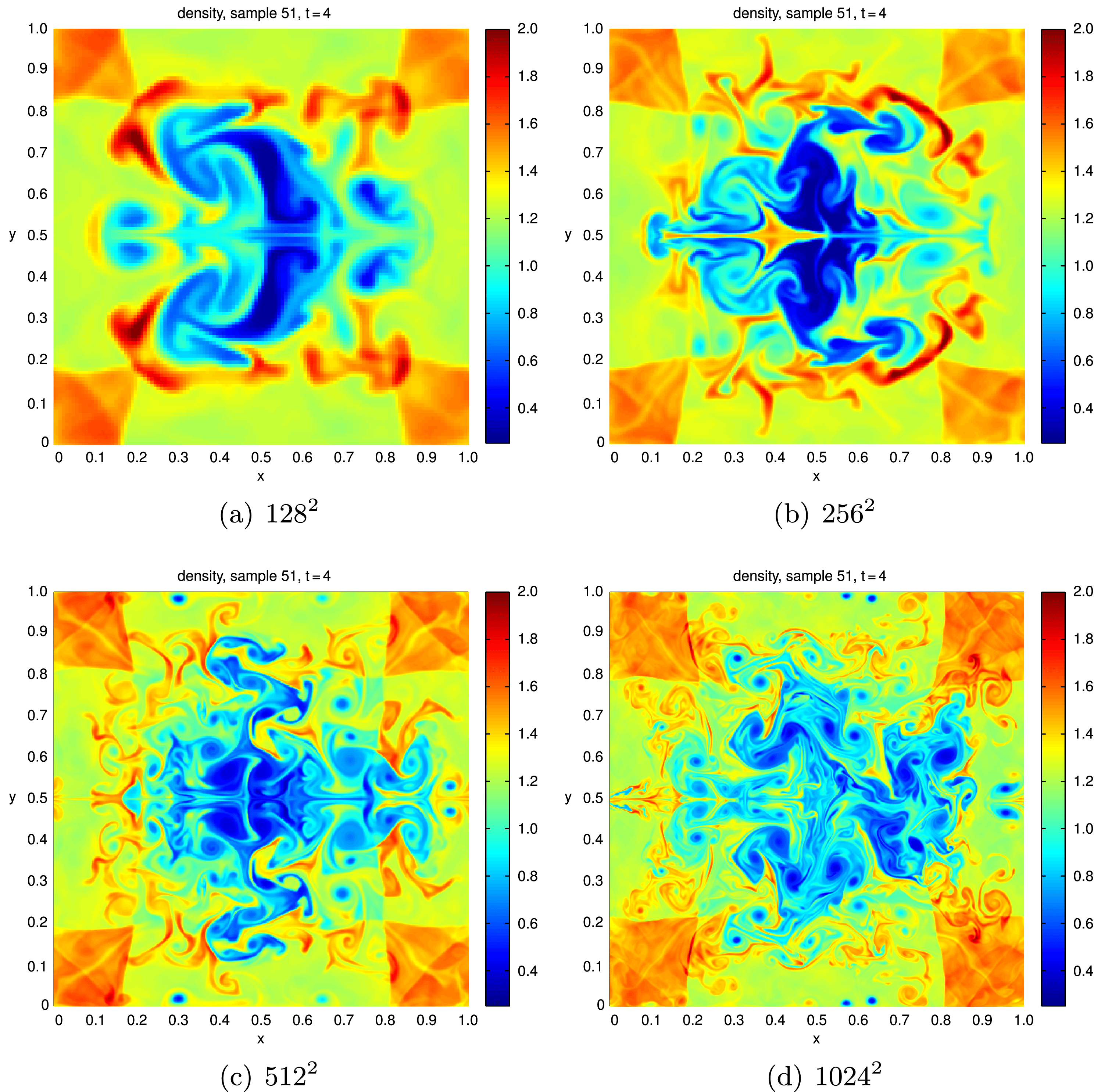
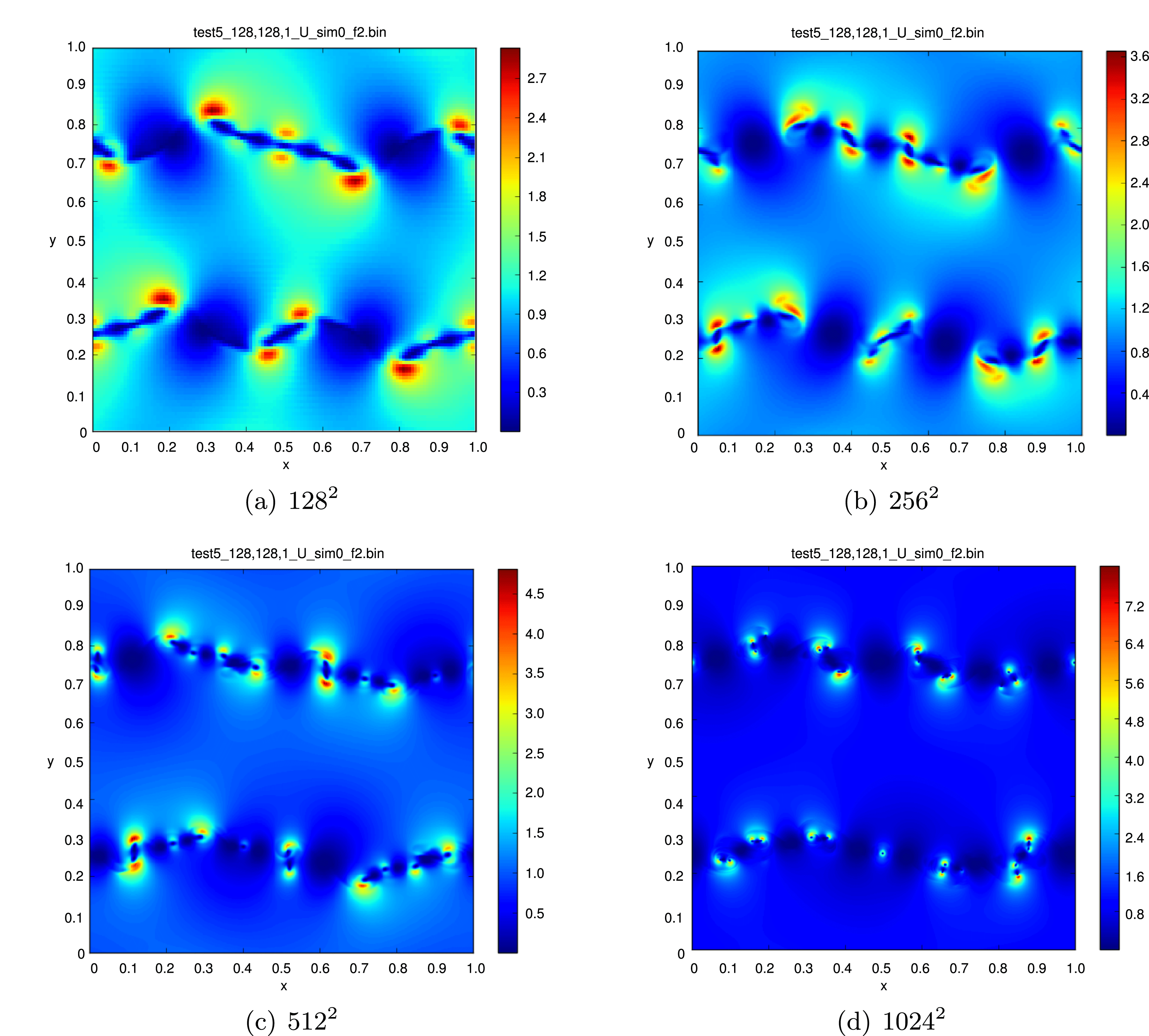
 $t=4$ is plotted in Figure 1.2. As shown in the figure, the solution is fairly complex: the initial shock waves generated from the explosion have exited and re-entered the domain (on account of periodic boundary conditions) and are interacting with an unstable interface. Furthermore, the re-entered shock creates a complex pattern of small-scale eddies on hitting the interface. These structures are formed at ever finer scales as the mesh is refined.
Initial data for the Richtmyer–Meshkov problem (7.2).
Approximate density at time  $t=4$ for a single sample, computed with the high-resolution finite volume scheme of Käppeli et al. (Reference Käppeli, Whitehouse, Scheidegger, Pen and Liebendörfer2011), for the Richtmyer–Meshkov problem (7.2) for different grid resolutions.


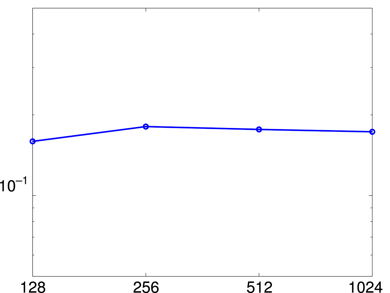
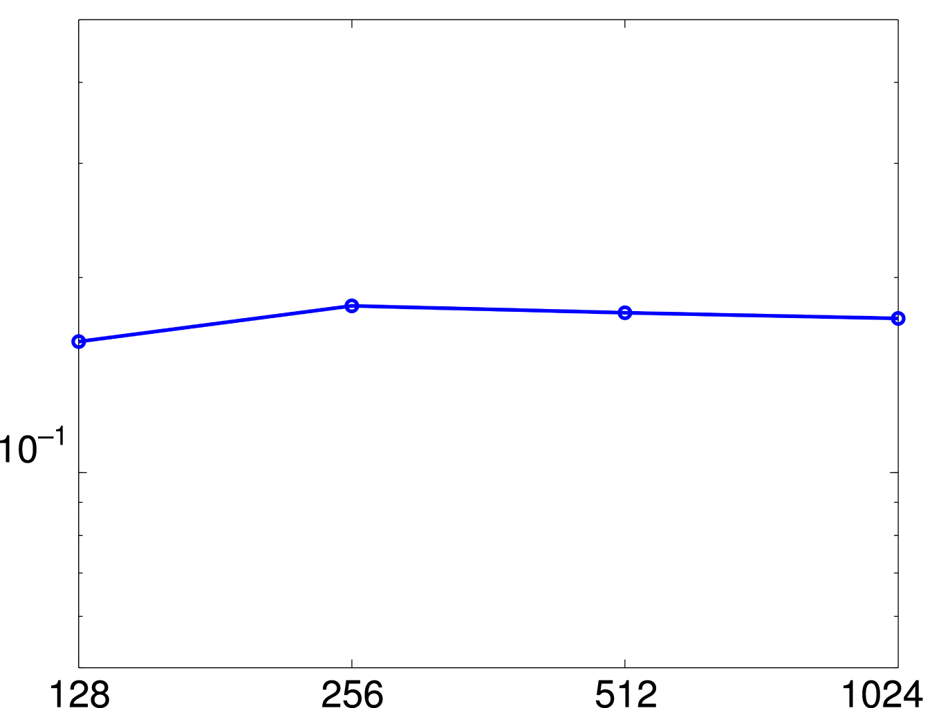
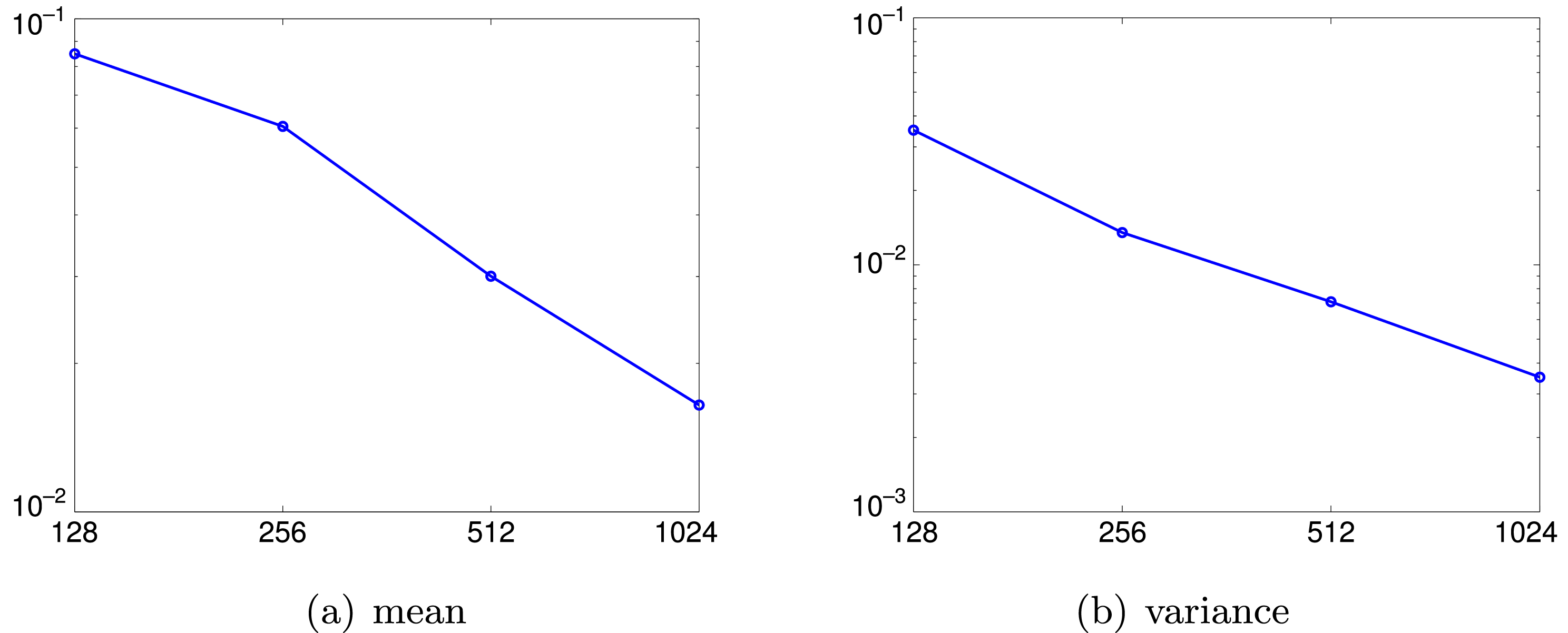
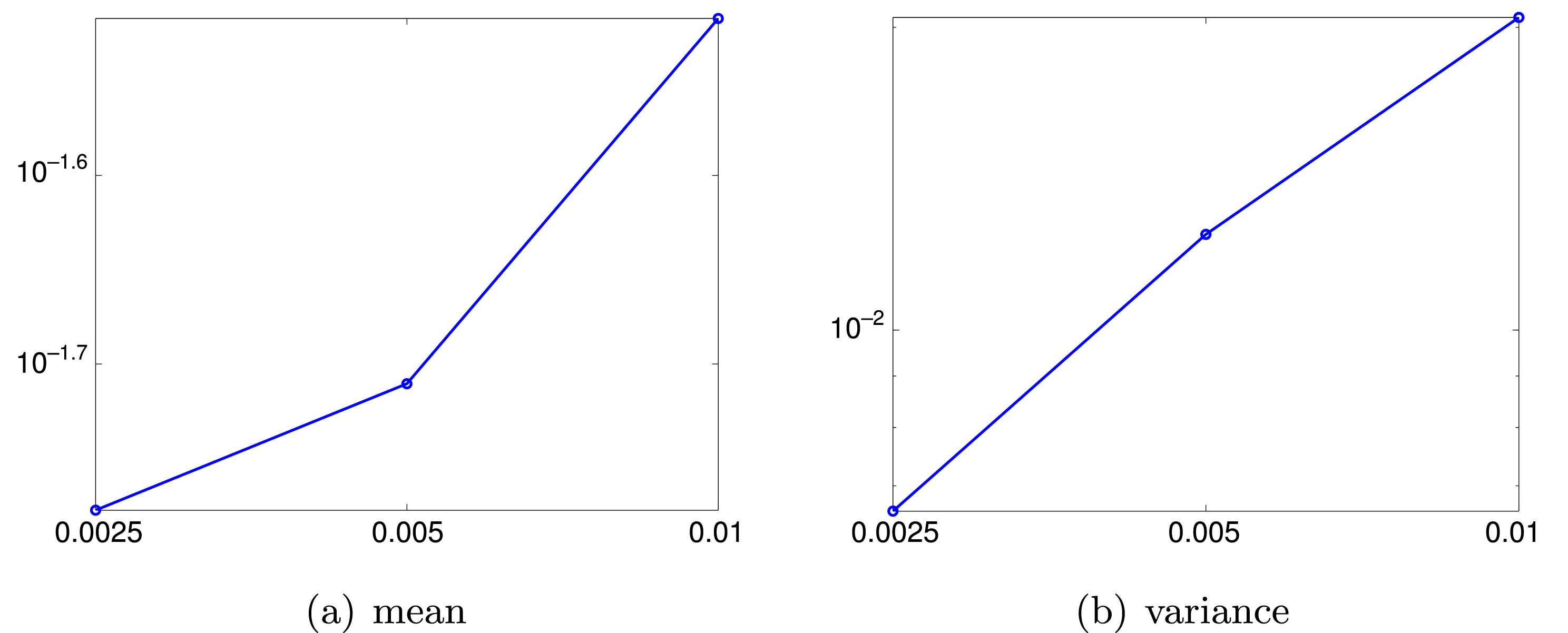
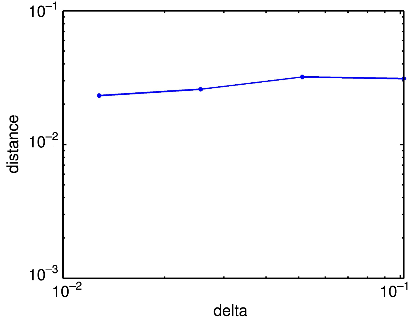
The appearance of structures at ever finer scales under mesh refinement may inhibit convergence of the scheme. To test this proposition, we compute the difference in the approximate solutions for two successive resolutions:
 $$\begin{eqnarray}{\mathcal{E}}^{N}=\Vert {\it\rho}^{2N}-{\it\rho}^{N}\Vert _{L^{1}([0,1]^{2})}.\end{eqnarray}$$
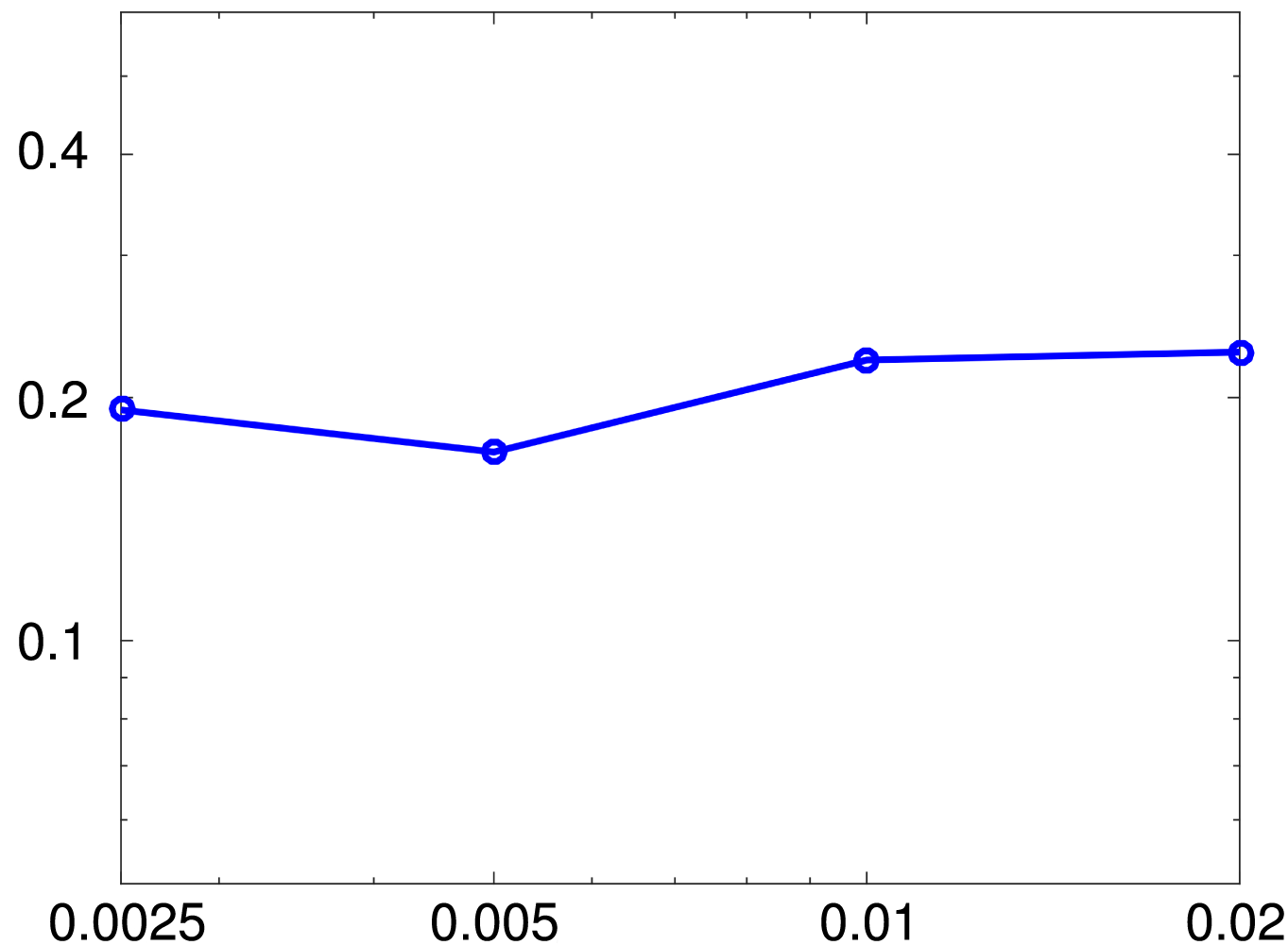
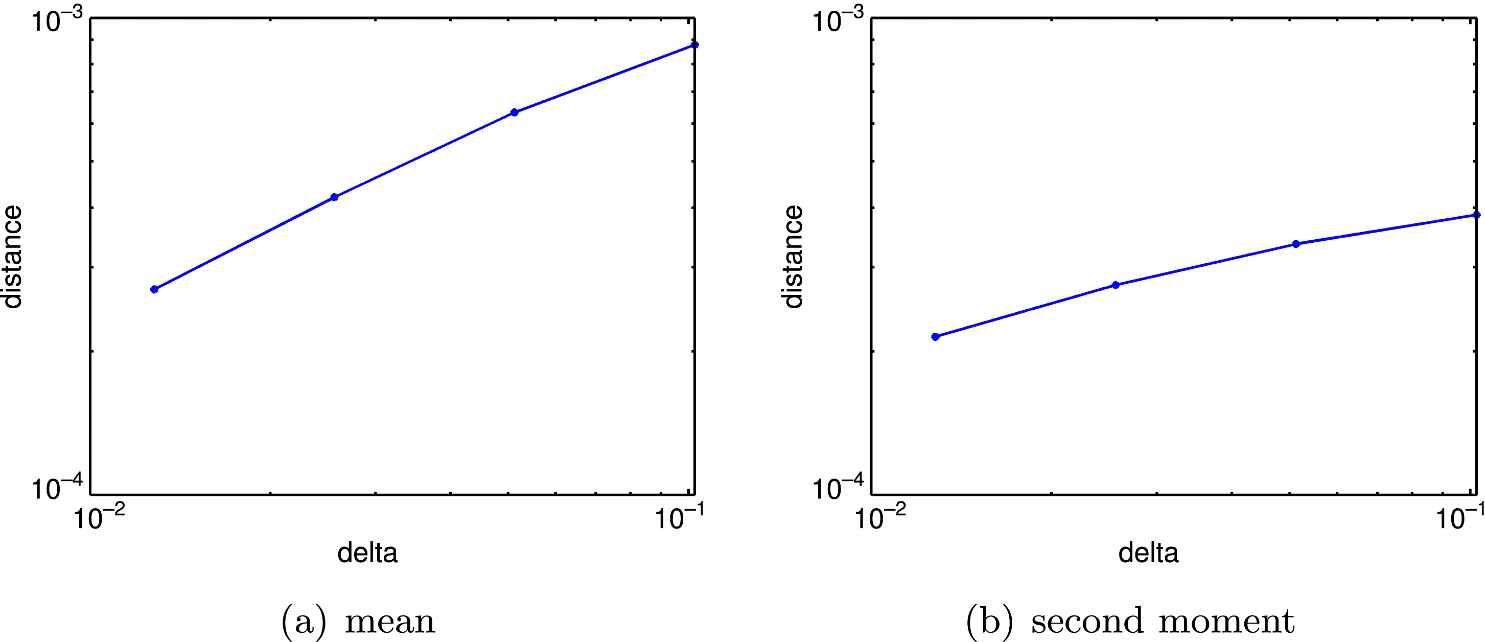
Here,  $N$ represents the number of mesh points in each direction. The results are shown in Figure 1.3 and demonstrate that the numerical approximation does not form a Cauchy sequence, let alone converge, as the mesh is refined. Similar results are also obtained with other
 $L^{p}$ norms. This lack of convergence is not an artifact of the scheme discussed here; as reported in Fjordholm, Käppeli, Mishra and Tadmor (Reference Fjordholm, Käppeli, Mishra and Tadmor2016a), very similar results have been obtained with other state-of-the-art schemes, such as the high-order TeCNO schemes (Fjordholm, Mishra and Tadmor Reference Fjordholm, Mishra and Tadmor2012) and WENO schemes (Fuchs et al. Reference Fuchs, McMurry, Mishra, Risebro and Waagan2011).
Is this non-convergent behaviour a feature of the compressible Euler equations only, or can it be observed in a larger class of PDEs? We address this question with another numerical example by considering the incompressible Euler equations, which model the motion of an ideal, inviscid incompressible fluid:
 $$\begin{eqnarray}\left\{\begin{array}{@{}r@{}}\partial _{t}u+{\rm\nabla}_{x}\cdot (u\otimes u)+{\rm\nabla}p=0,\\ {\rm\nabla}_{x}\cdot u=0.\end{array}\right.\end{eqnarray}$$
Here,  $u$ is the divergence-free velocity field,
 $u(\cdot ,t):D\subset \mathbb{R}^{d}\rightarrow \mathbb{R}^{d}$, and the pressure
 $p$ acts as a Lagrange multiplier to impose the divergence-free constraint.
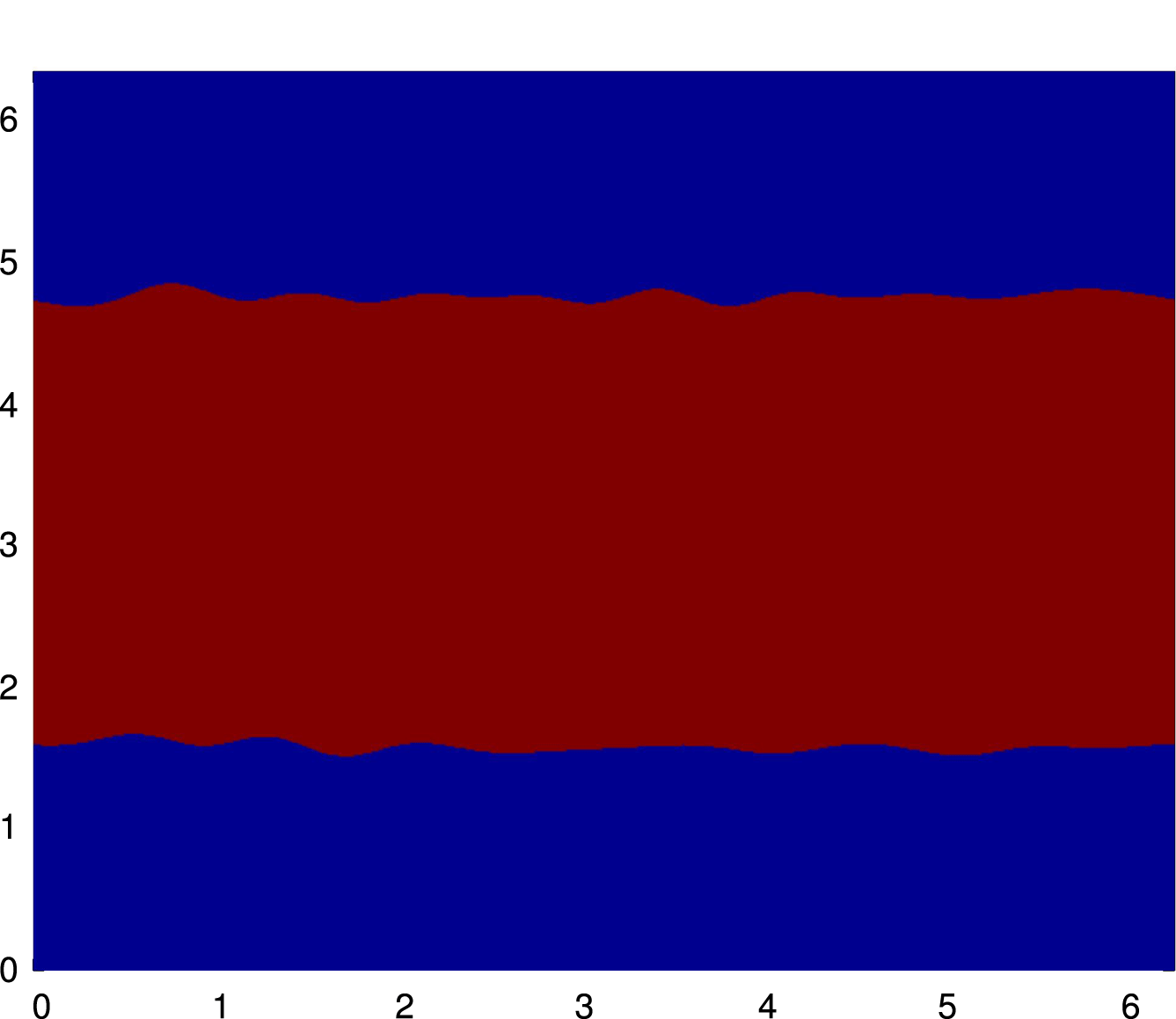
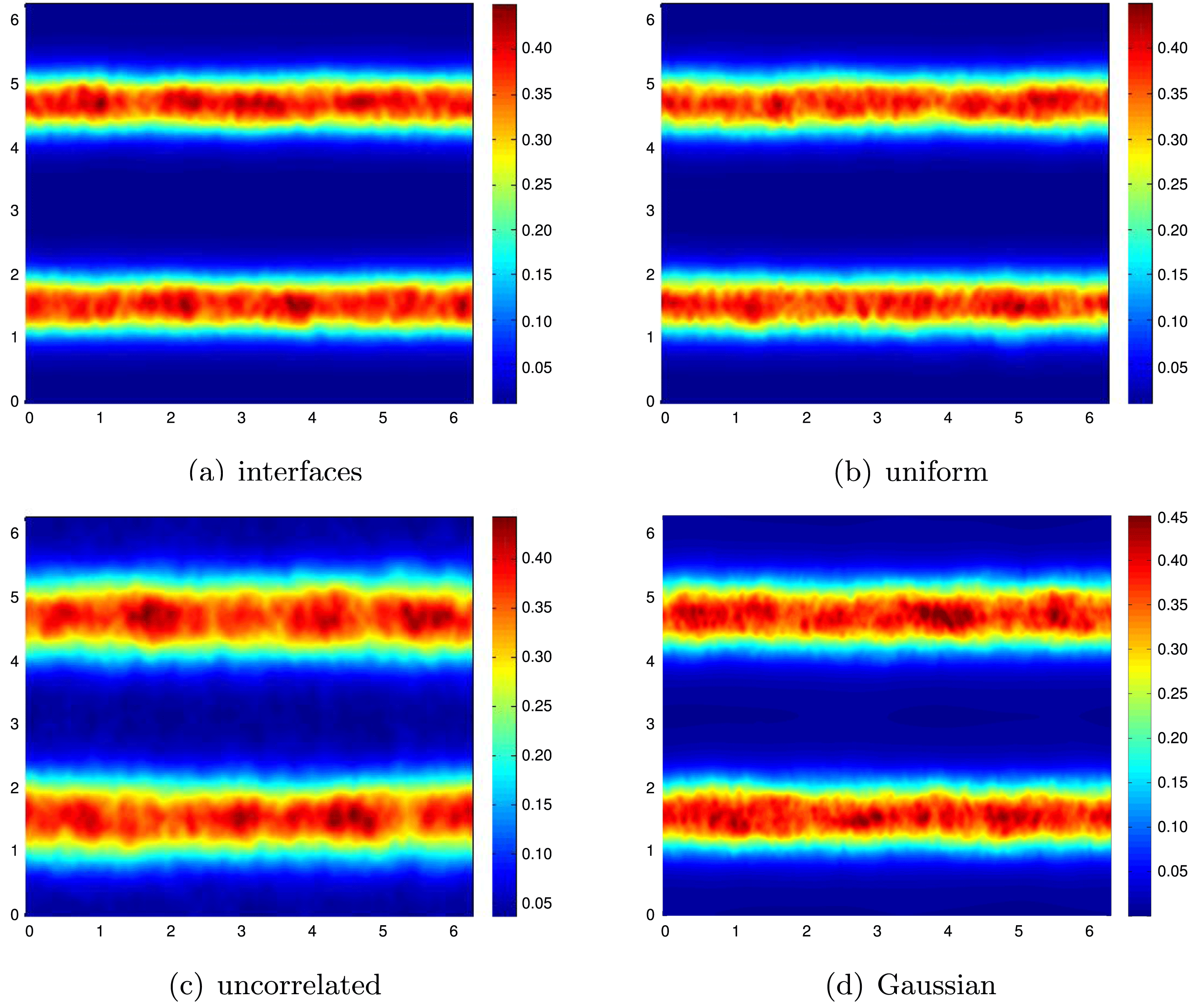
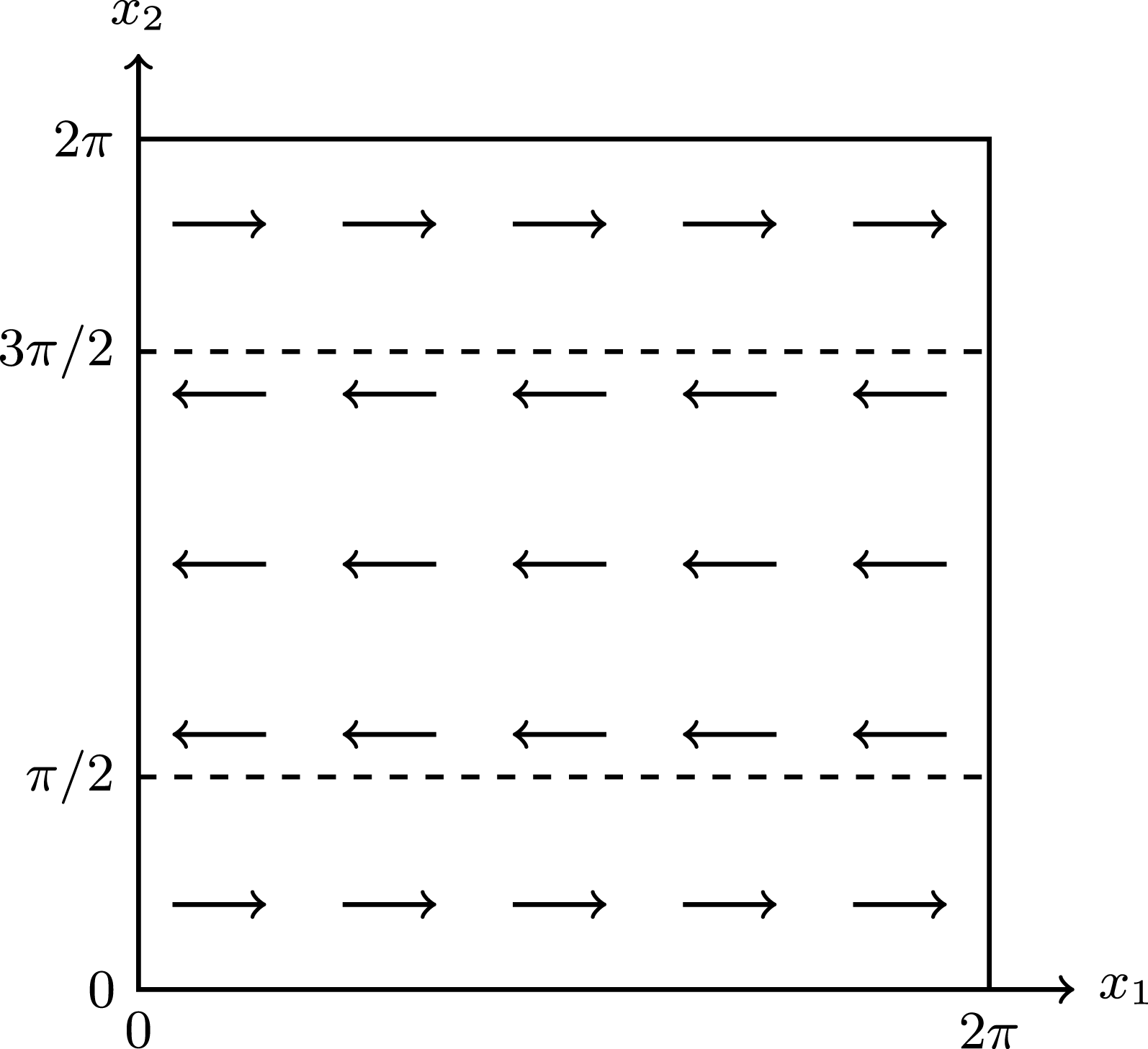
We consider the two-dimensional version ( $d=2$) of the incompressible Euler equations (1.3) in the two-dimensional periodic torus
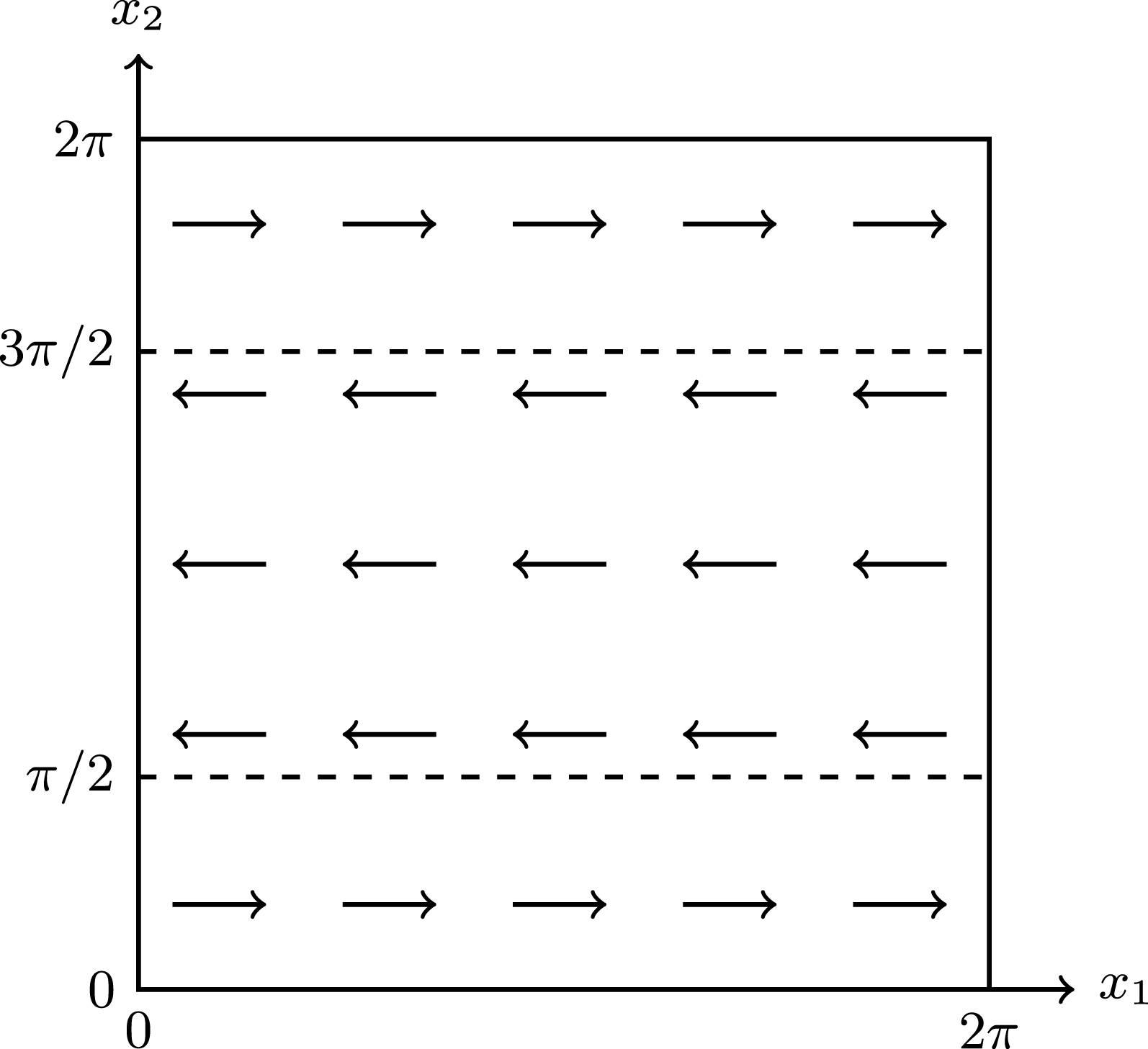
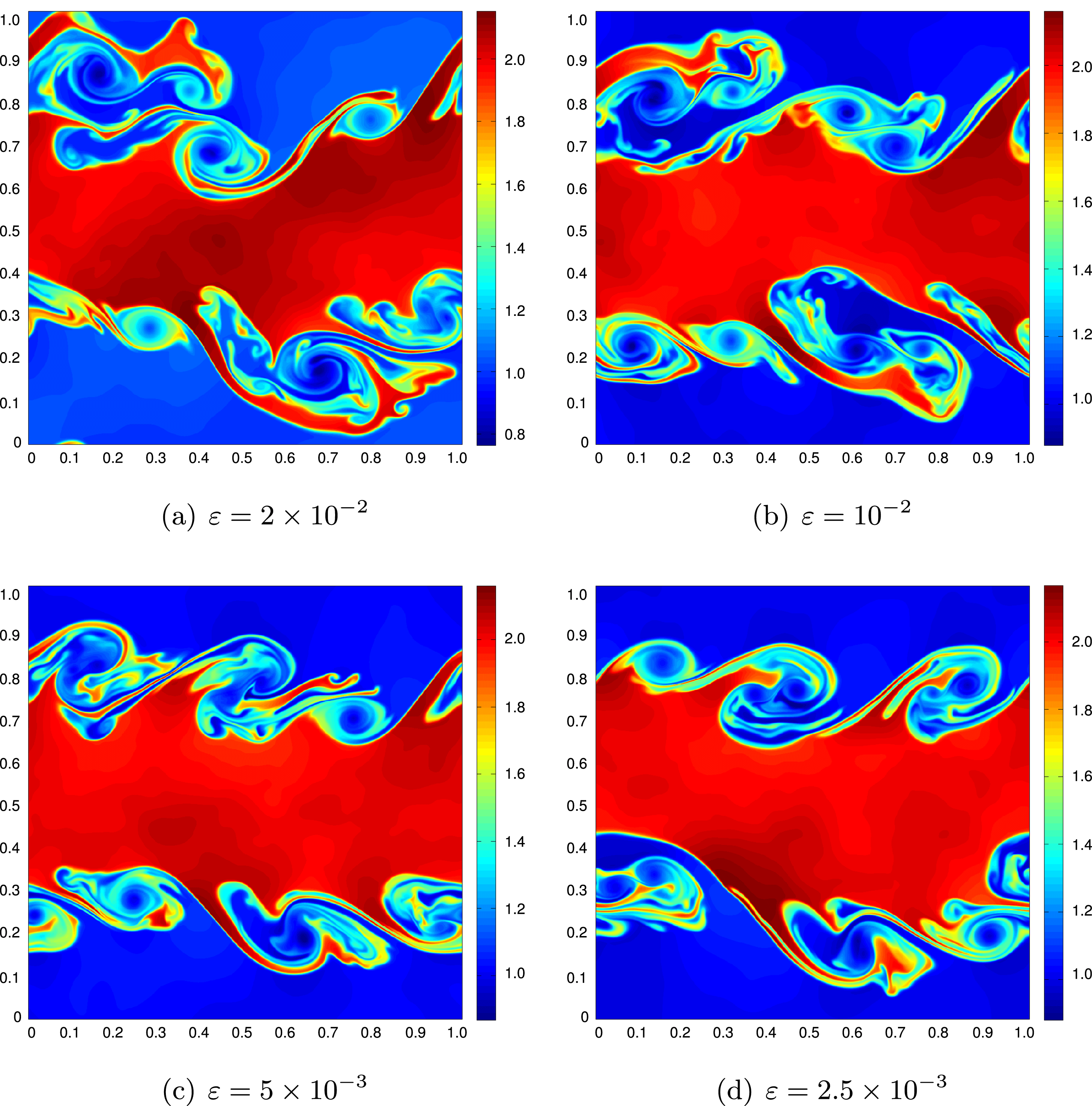
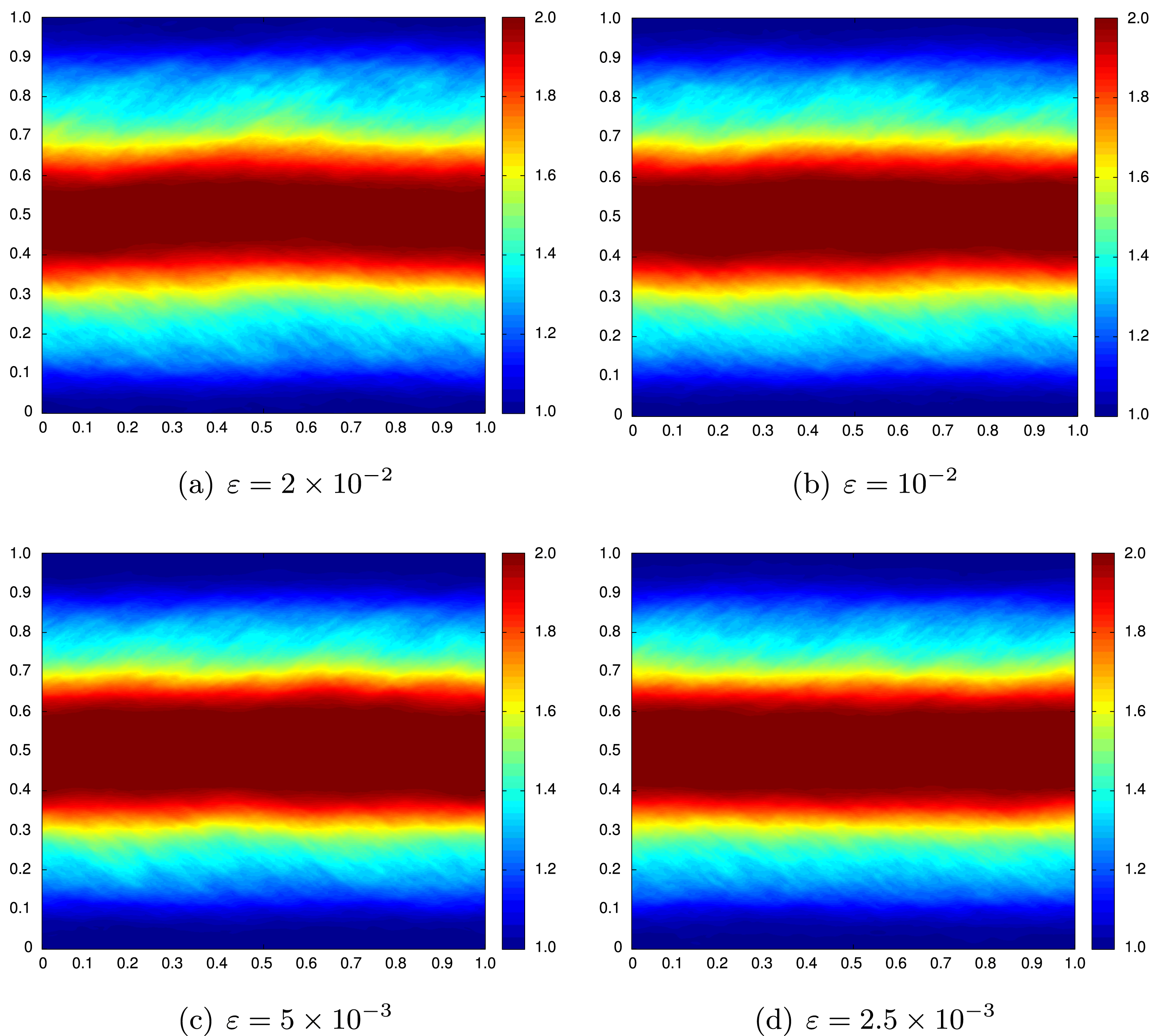
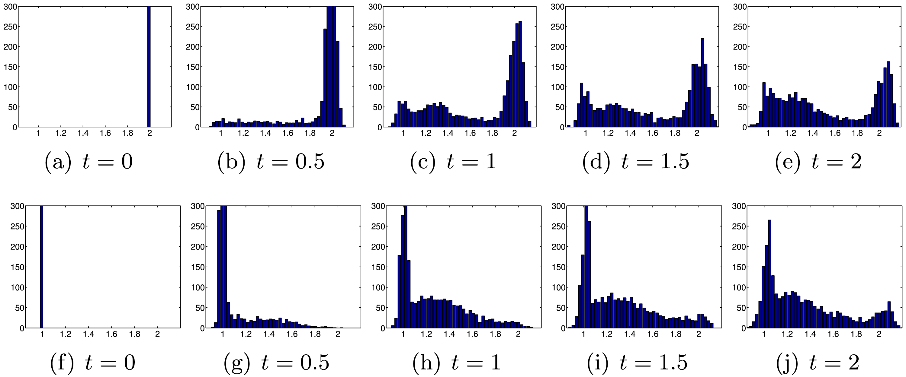
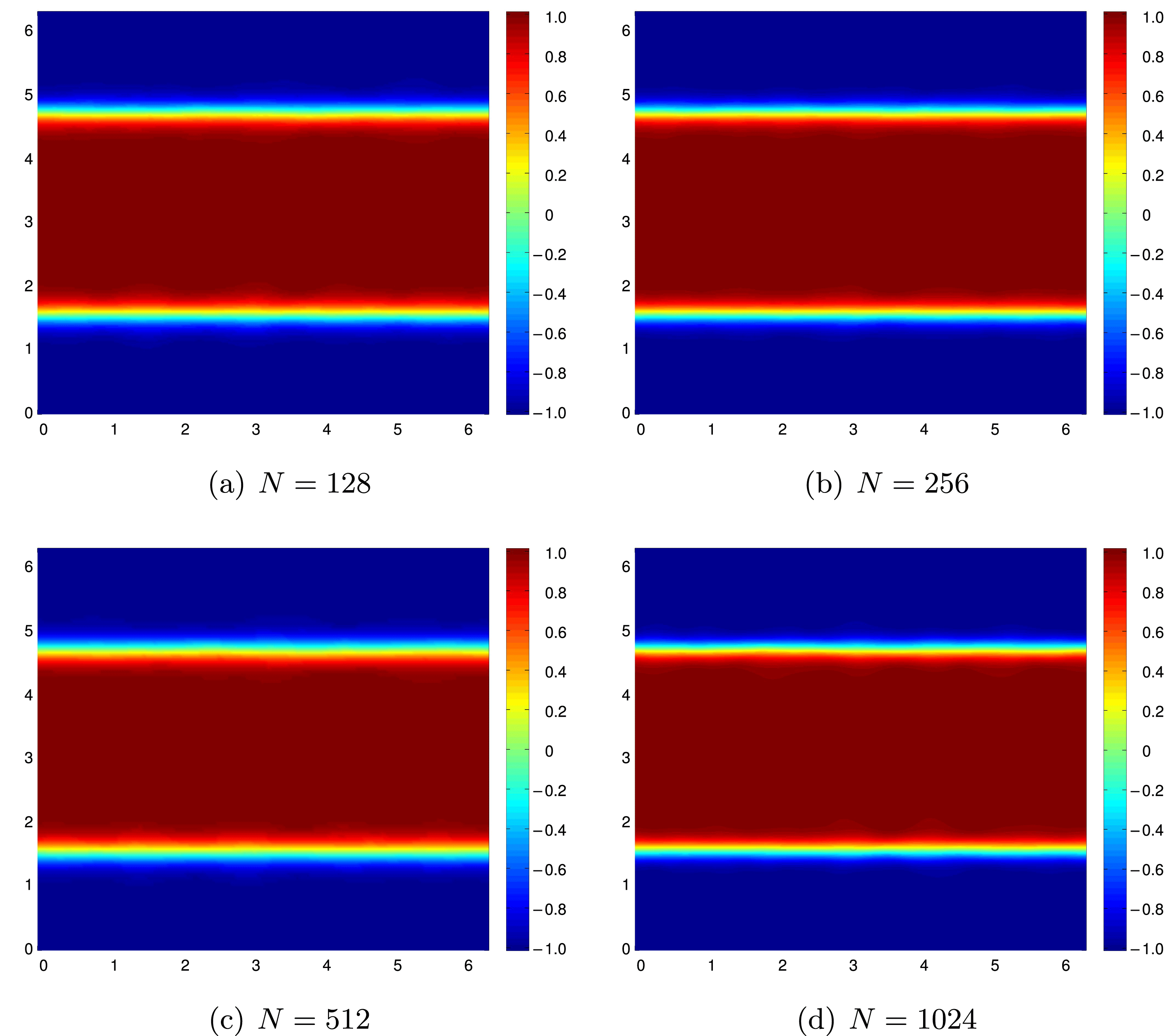
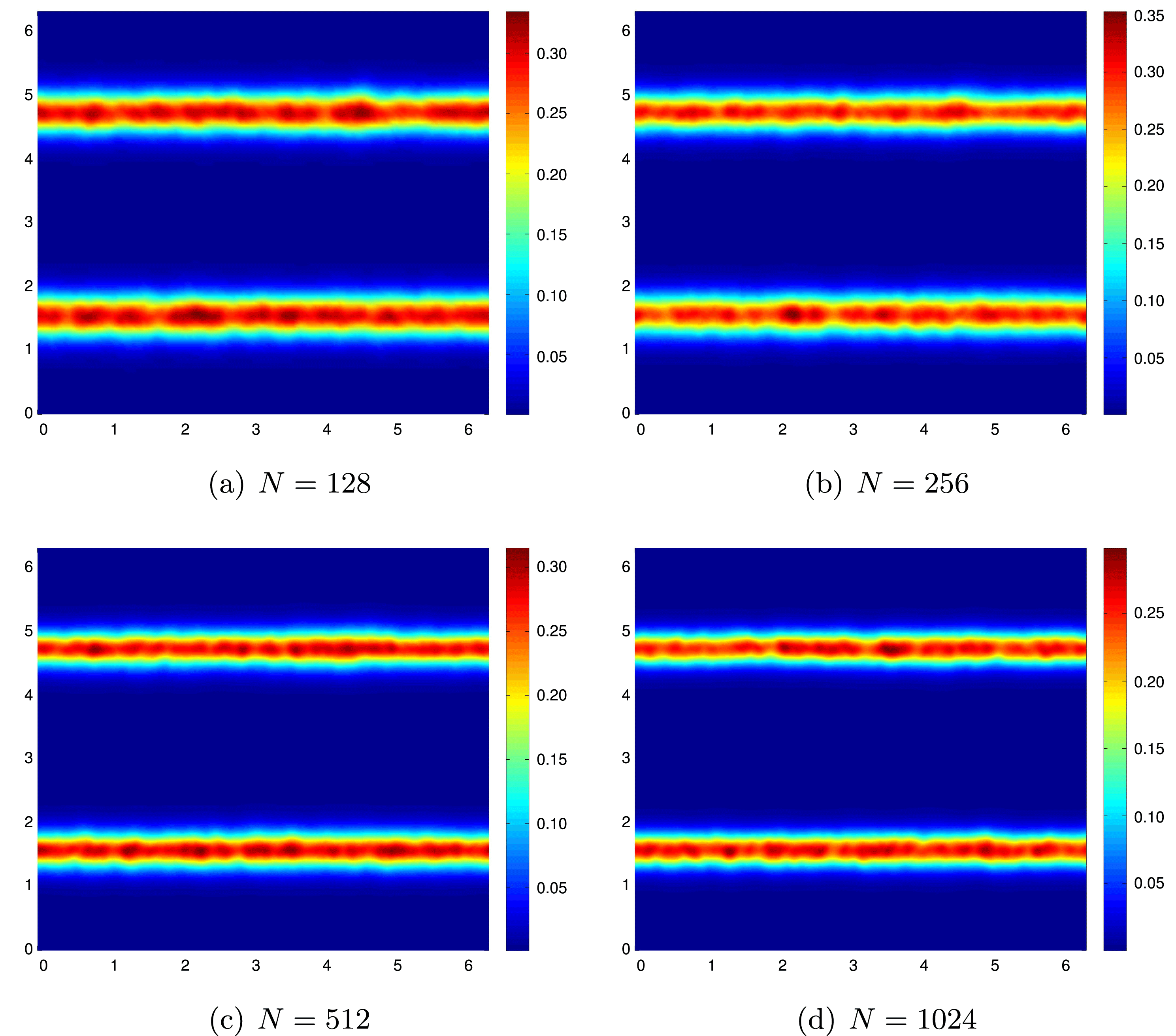
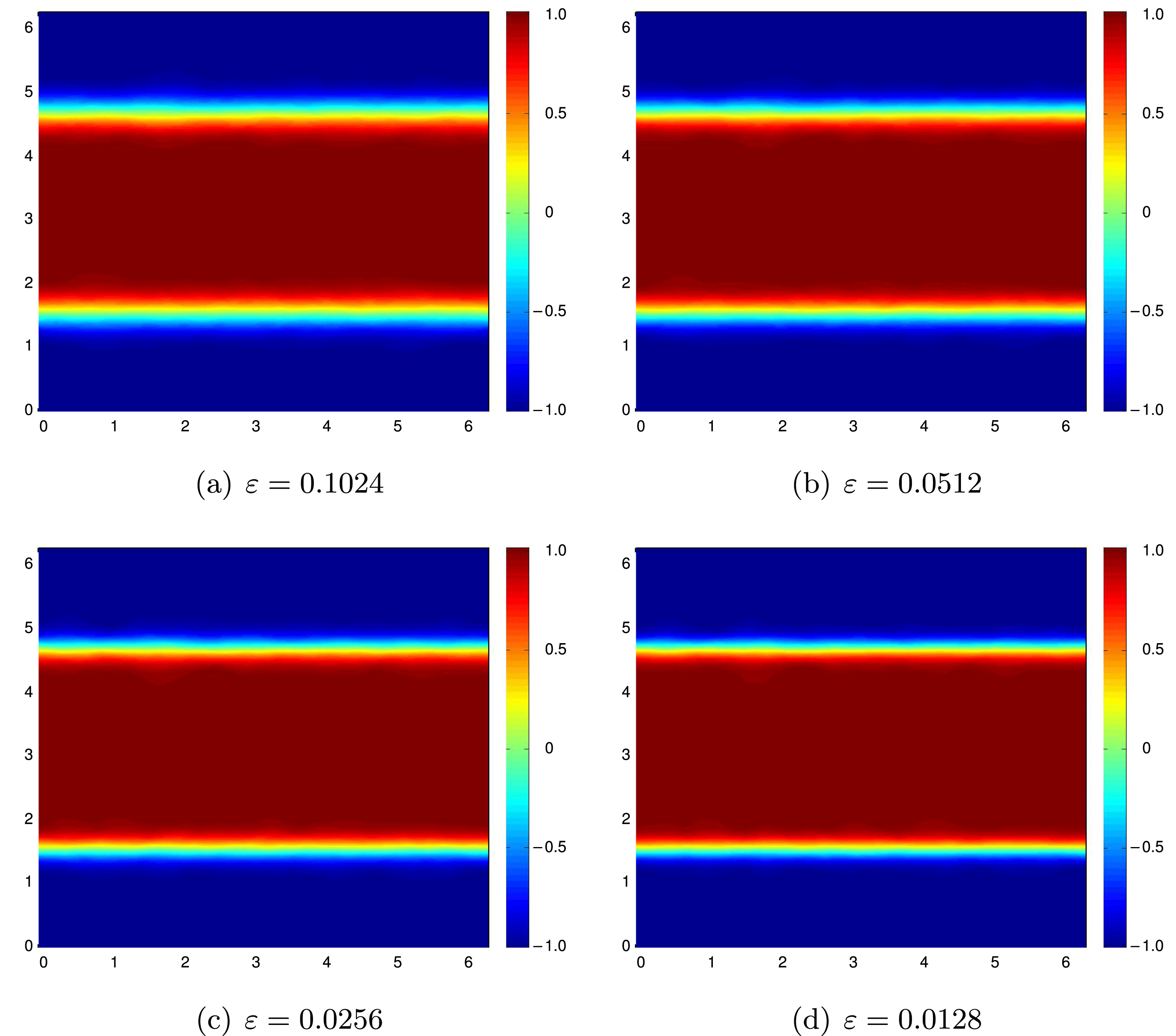
 $D=[0,2{\it\pi}]^{2}$ with initial data shown in Figure 1.4 (see also (8.1)). The initial datum is a (slightly) perturbed version of the two-dimensional flat vortex sheet. We approximate this problem numerically with a widely used spectral method; see Section 4 and Gottlieb, Hussaini and Orszag (Reference Gottlieb, Hussaini, Orszag and Voigt1984). We compute a sequence of approximate solutions with an increasing number of Fourier modes ranging from
 $N=128$ to
 $N=1024$. In order to visualize the resulting solution, we plot the pointwise (in the spatial domain) kinetic energy
 $u_{1}^{2}+u_{2}^{2}$ at time
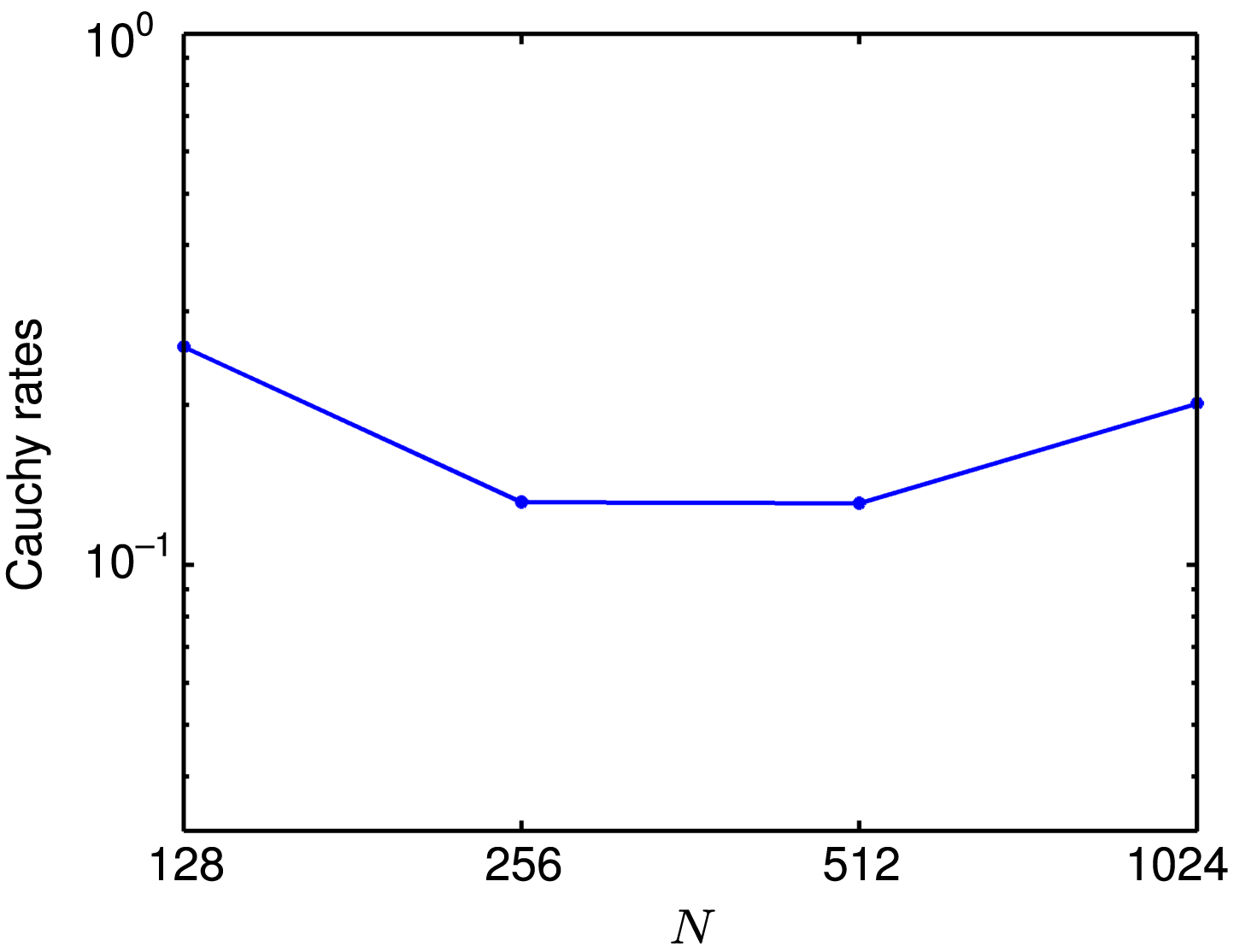
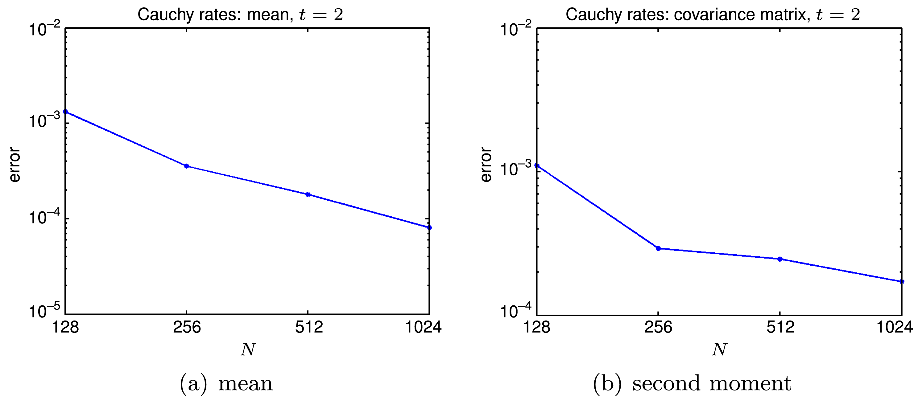
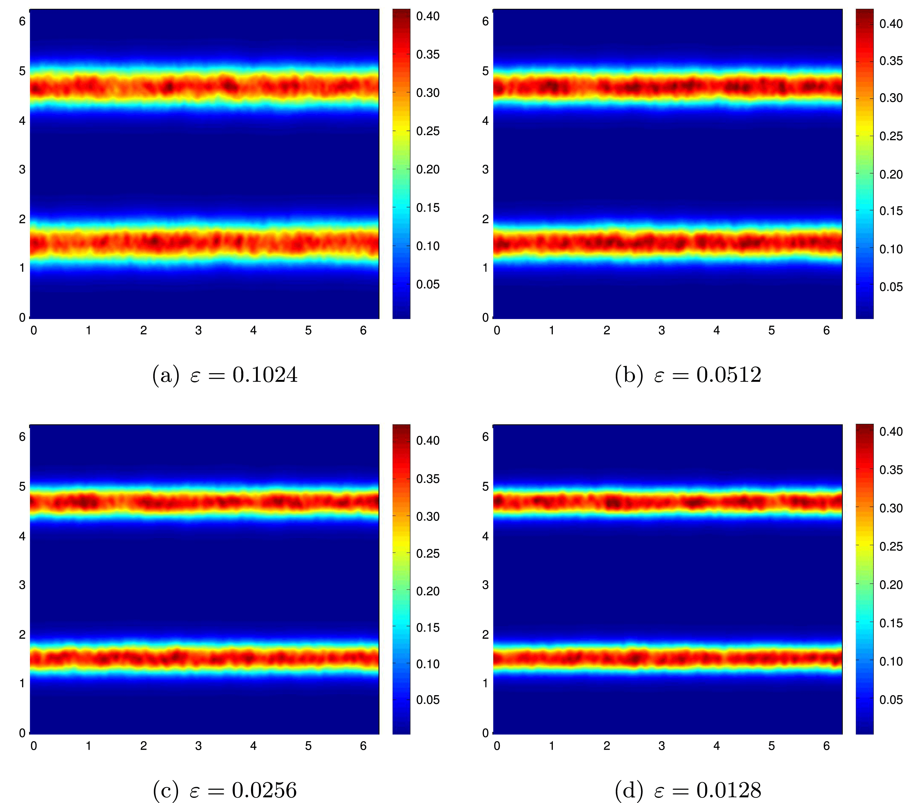
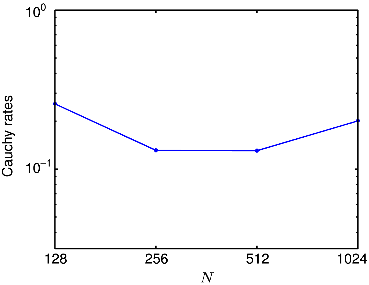
 $t=2$ in Figure 1.5. As the figure shows, the local energy appears to be concentrated (distributed) on smaller-scale structures as the number of Fourier modes is increased. This suggests a lack of convergence of the approximation, which we further quantify in terms of ‘Cauchy rates’ – the difference in the approximate (velocity) solutions on successive resolutions:
 $$\begin{eqnarray}{\mathcal{E}}^{N}=\Vert u^{2N}-u^{N}\Vert _{L^{2}([0,2{\it\pi}]^{2})}.\end{eqnarray}$$
We plot this difference in Figure 1.6. The figure clearly shows that there is no convergence for the spectral method in this case, as the difference in successive approximations remains  $O(1)$ with increasing resolution. Similar non-convergent results have also been obtained with a spectral viscosity method (Lanthaler and Mishra Reference Lanthaler and Mishra2015) and with a finite difference projection method (Leonardi and Mishra Reference Leonardi and Mishra2016).
Initial data for the perturbed vortex sheet (8.1).



The two numerical experiments presented above consider two different types of non-linear systems of PDEs as well as very different numerical methods, one a finite volume scheme and the other a spectral approximation. Still, they both illustrate the phenomenon of lack of convergence of numerical approximations as the resolution is increased. This non-convergence can be attributed to at least two phenomena:
∙ the appearance of oscillations at ever finer scales as the mesh is refined,
∙ the unstable behaviour of these oscillations with respect to mesh resolution, numerical method, small initial perturbations, etc.
These phenomena are not new, and have already manifested themselves in past computation of ill-posed problems, such as the prototype example of incompressible motion of perturbed vortex sheets. Computation of the underlying Kelvin–Helmholtz instability necessitates an increasingly finer resolution involving  $N$ degrees of freedom, which leads to faster noise amplification of order
 $e^{Nt/2}$. Several methodologies were developed to address this phenomenon by containing noise amplification to below machine accuracy, as in the meticulous computations of Krasny (Reference Krasny1986a, Reference Krasny1986b), who was the first to compute beyond critical time of singularity formation. But errors of different orders and uncertainties of different sources are here to stay, and as noted by Majda and Bertozzi (Reference Majda and Bertozzi2002, p. 371), the phenomenon of their prohibitive growth ‘is a feature of the underlying equation itself as opposed to an instability of the numerical method.’
It seems that the current notions of weak solutions for these equations, based on integrable functions, do not suffice to describe the limits of widely used numerical approximations for such problems. This raises the question whether there exists a suitable framework of solutions for these classes of non-linear PDEs which can accommodate solutions with unstable oscillations at arbitrarily small scales, as illustrated in their numerical approximation. We postulate that measure-valued solutions, first proposed by DiPerna (Reference DiPerna1985), can provide an appropriate solution paradigm for the analysis and computation of these large classes of non-linear PDEs.
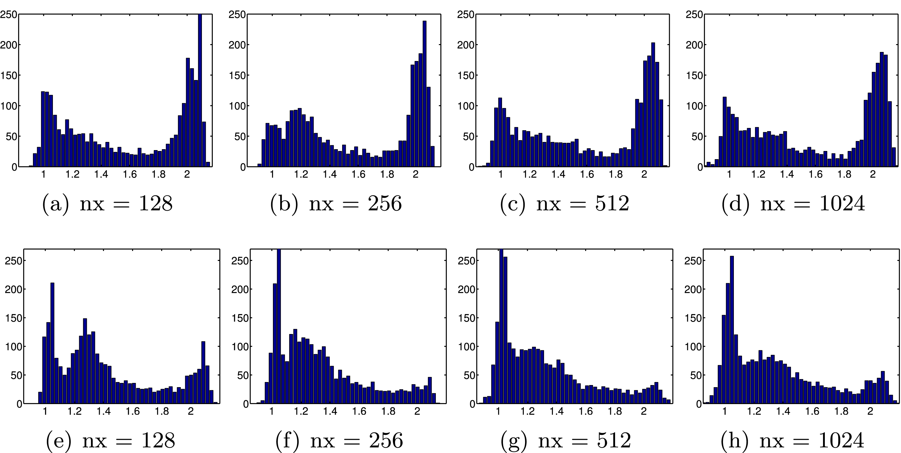
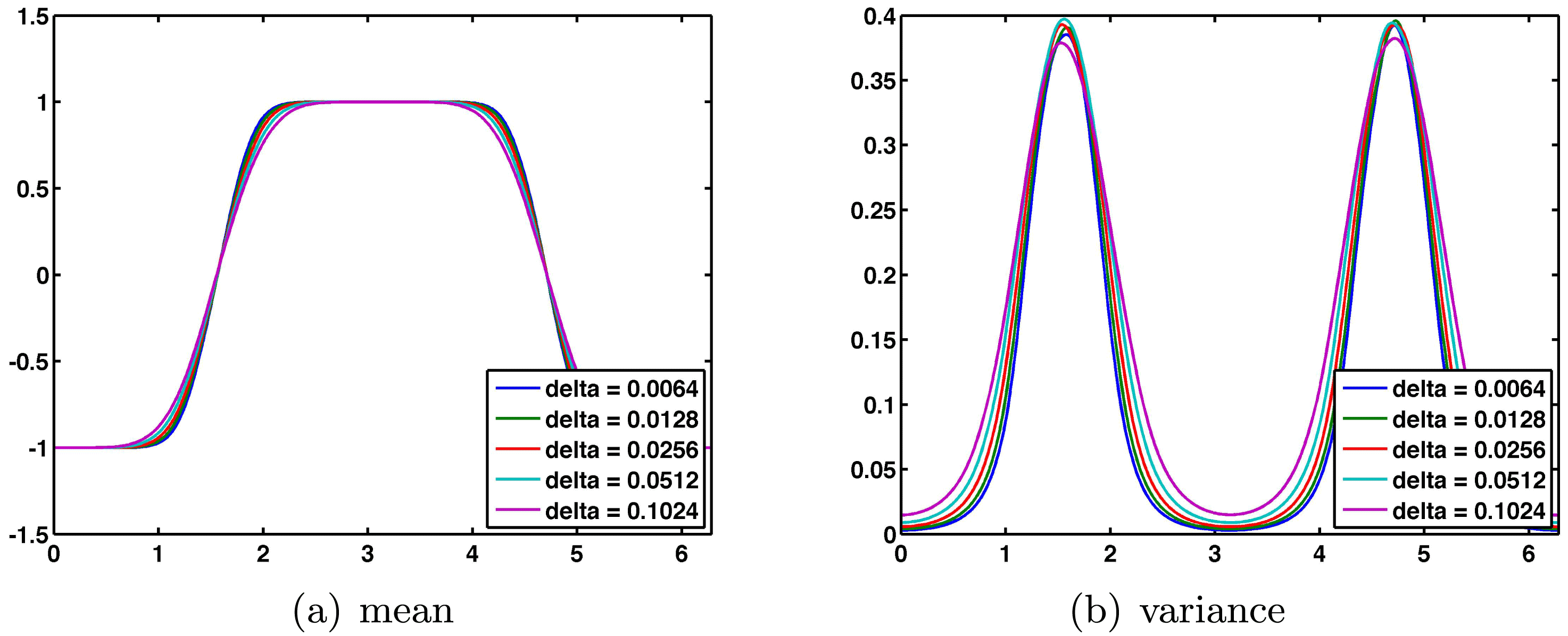
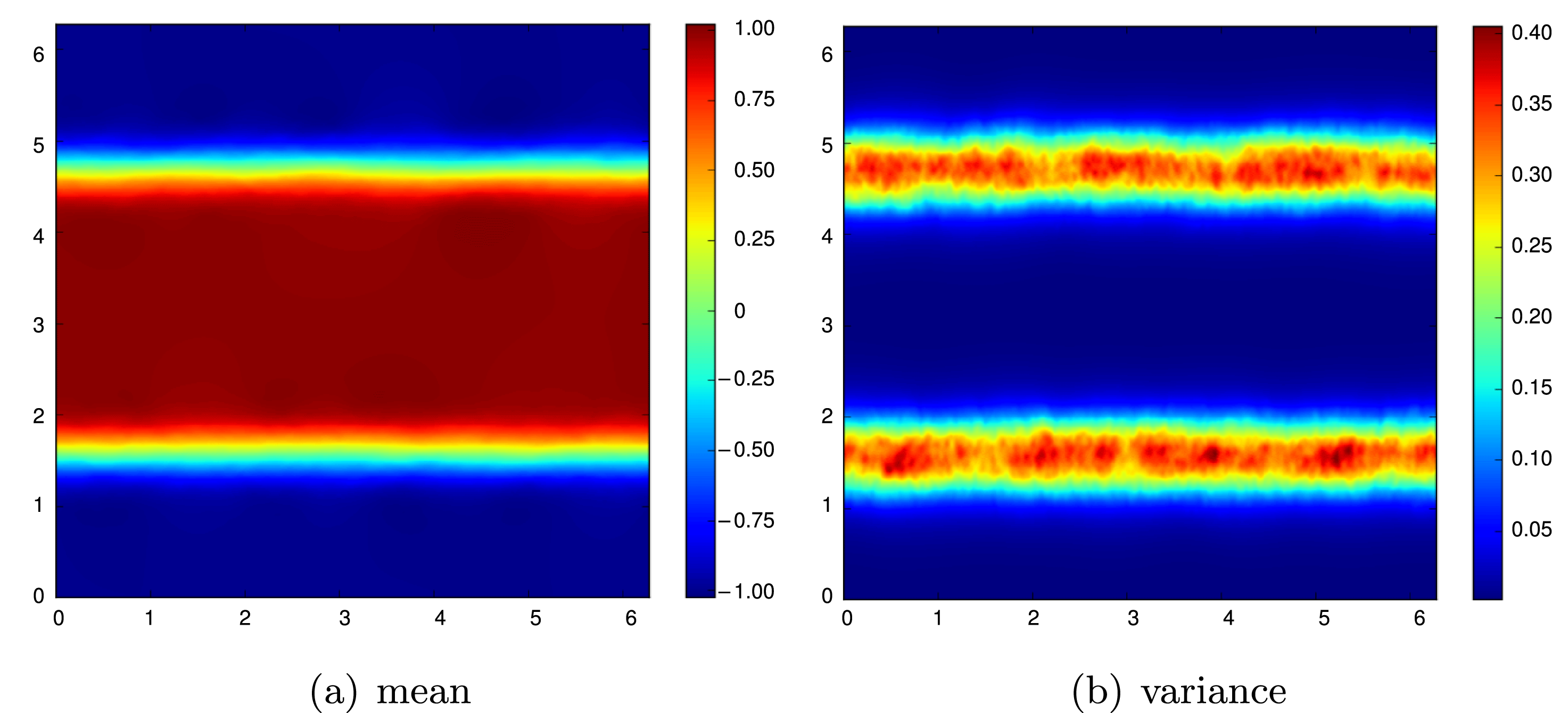
Although measure-valued solutions have been available for the past thirty years and many theoretical results have been established (Demoulini, Stuart and Tzavaras Reference Demoulini, Stuart and Tzavaras2012, DiPerna and Majda Reference DiPerna and Majda1987a, Frid and Liu Reference Frid and Liu1998, Reference Frid and Liu1995, Panov Reference Panov1994, Reference Panov1993, Kröner and Zajaczkowski Reference Kröner and Zajaczkowski1996, Málek, Nečas, Rokyta and Ružička Reference Málek, Nečas, Rokyta and Ružička1996, Schochet Reference Schochet1989, Székelyhidi Jr and Wiedemann Reference Székelyhidi and Wiedemann2012), the computation of measure-valued solutions is fairly recent. Algorithms for computing measure-valued solutions in the context of turbulent mixing were proposed by Glimm and co-workers (Glimm, Grove and Zhang Reference Glimm, Grove and Zhang1999, Lim et al. Reference Lim, Yu, Glimm, Li and Sharp2008), and were discussed in Roy and Acharya (Reference Roy and Acharya2006, p. 1730) in the context of mesoscopic field dislocation mechanics. However, rigorous convergence analysis of these algorithms is not available. Fjordholm et al. (Reference Fjordholm, Käppeli, Mishra and Tadmor2016a) have proposed a novel algorithm for computing entropy measure-valued solutions of the compressible Euler equations (1.1), as a prototype example of the larger class of systems of conservation laws (reviewed in Section 2.1 below). The algorithm, which is outlined in Section 4 below, realizes the underlying Young measures as laws of Monte Carlo-sampled random fields and, under verifiable assumptions on the space-time discretizations, has been proved to converge to an entropy measure-valued solution of the system of conservation laws in question. Lanthaler and Mishra (Reference Lanthaler and Mishra2015) have extended the algorithm to compute admissible measure-valued solutions of the incompressible Euler equations (1.3) (reviewed in Section 2.2 below). Most notably, unlike the computations of weak solutions shown in Figures 1.3 and 1.6, the errors of these measure-valued computations do decrease under mesh refinement, which demonstrates that numerical approximations converge to measure-valued – rather than weak – solutions of the compressible and incompressible Euler equations. Thus, measure-valued solutions (and suitable variants thereof) may serve as an appropriate solution paradigm for these PDEs.
The aim of the current paper is to review these algorithms for computing measure-valued solutions, present them within a unified framework, illustrate them with a large number of numerical experiments, and discuss shortcomings as well as extensions of these algorithms. To this end, we organize the rest of the paper as follows. In Section 2 we provide a brief review of theoretical developments, in the context of admissible weak solutions, for both systems of conservation laws and incompressible Euler equations. The definitions of Young measures and measure-valued solutions are presented in Section 3. In Section 4 we present algorithms to compute measure-valued solutions and discuss convergence of these algorithms. In Sections 5 and 6, respectively, these algorithms are used to compute approximate measure-valued solutions for systems of conservation laws and for the incompressible Euler equations. Numerical experiments are presented in Sections 7 and 8. The question of uniqueness (stability) of measure-valued solutions, the related framework of statistical solutions and its significance for uncertainty quantification are discussed in Sections 9 and 10. In Section 11 we present other algorithms, particularly of the multi-level Monte Carlo type, to approximate measure-valued solutions. The use of Young measures in materials science is discussed in Section 12.
2 A brief review of theoretical results
Our main goal in this paper is to present efficient, convergent algorithms for computing measure-valued solutions of certain classes of non-linear PDEs. As mentioned in the Introduction, we focus on two specific classes of PDEs: systems of conservation laws (with the compressible Euler equations (1.1) being the prototypical example) and the incompressible Euler equations (1.3). In order to provide the context for the approximation of measure-valued solutions for these PDEs, we collect some of the available theoretical results for these PDEs in the following. Our focus is on the main results of well-posedness, that is, those of (global) existence, uniqueness and stability.
2.1 Systems of conservation laws
The system of compressible Euler equations (1.1) is the prototypical example of the class of systems of conservation laws which take the generic form
 $$\begin{eqnarray}\begin{array}{@{}rl@{}}\partial _{t}u+{\rm\nabla}_{x}\cdot f(u)=0, & (x,t)\in \mathbb{R}^{d}\times \mathbb{R}_{+},\\ u(x,0)=u_{0}(x), & x\in \mathbb{R}^{d}.\end{array}\end{eqnarray}$$
Here,  $u=u(x,t):\mathbb{R}^{d}\times \mathbb{R}_{+}\rightarrow \mathbb{R}^{N}$ is the unknown vector of conserved variables dictated by the flux functions
 $f=(f^{1},\ldots ,f^{d}):\mathbb{R}^{N}\rightarrow \mathbb{R}^{N\times d}$, and the goal is to identify the solution which evolves over time,
 $u_{0}(\cdot )\mapsto u(\cdot ,t)$ for
 $t\in \mathbb{R}_{+}:=[0,\infty )$.
In this section we recall some of the theoretical results for systems of conservation laws which will be needed below. Much of the theory for such systems was driven by the example of compressible Euler equations (1.1) with  $u=({\it\rho},{\it\rho}v,E)^{\top }$, expressing the conservation of the density
 ${\it\rho}$, momentum
 $m:={\it\rho}v$ and energy
 $E$. We begin with the definition of weak solutions for (2.1).
Definition 2.1. A function  $u\in L^{\infty }(\mathbb{R}^{d}\times \mathbb{R}_{+},\mathbb{R}^{N})$ is a weak solution of (2.1) if it satisfies (2.1) in the sense of distributions:
 $$\begin{eqnarray}\int _{\mathbb{R}_{+}}\int _{\mathbb{R}^{d}}\partial _{t}{\it\varphi}(x,t)u(x,t)+{\rm\nabla}_{x}{\it\varphi}(x,t)\cdot f(u(x,t))\,\text{d}x\,\text{d}t+\int _{\mathbb{R}^{d}}{\it\varphi}(x,0)u_{0}(x)\,\text{d}x=0\end{eqnarray}$$
for all test functions  ${\it\varphi}\in C_{c}^{1}(\mathbb{R}^{d}\times \mathbb{R}_{+})$.
Weak solutions are not necessarily unique. We need to specify additional admissibility conditions in order to select physically meaningful weak solutions. These take the form of entropy conditions (Lax Reference Lax and Zarantonello1971), given in terms of entropy pairs.
Definition 2.2. A pair of functions  $({\it\eta},q)$ with
 ${\it\eta}:\mathbb{R}^{N}\rightarrow \mathbb{R}$,
 $q:\mathbb{R}^{N}\rightarrow \mathbb{R}^{d}$ is called an entropy pair if
 ${\it\eta}$ is convex and
 $q$ satisfies the compatibility condition
 $q^{\prime }={\it\eta}^{\prime }\cdot f^{\prime }$, that is,
 $$\begin{eqnarray}{\rm\nabla}_{u}q_{i}(u)^{\top }={\rm\nabla}_{u}{\it\eta}(u)^{\top }{\rm\nabla}_{u}f_{i}(u)\end{eqnarray}$$
for  $i=1,\ldots ,d$ and all
 $u\in \mathbb{R}^{N}$.
The notion of entropy pairs is driven by the example of compressible Euler equations (1.1), which are equipped with a family of entropy pairs  $({\it\eta},q)=(-{\it\rho}h(s),-{\it\rho}vh(s))$, where the specific entropy is given by
 $s:=\ln (p{\it\rho}^{-{\it\gamma}})$. The convexity of
 ${\it\eta}={\it\eta}({\it\rho},m,E)$ is attained, for example, with the canonical pair
 $h(s)=s$. The behaviour of Euler entropic solutions as a limiting case for the Navier–Stokes equations motivates the following condition; see Godunov (Reference Godunov1961), Kružkov (Reference Kružkov1970, Section 7) and Lax (Reference Lax and Zarantonello1971).
Definition 2.3. A weak solution  $u$ of (2.1) is an entropy solution if the entropy inequality
 $$\begin{eqnarray}\partial _{t}{\it\eta}(u)+{\rm\nabla}_{x}\cdot q(u)\leq 0\quad \text{in }{\mathcal{D}}^{\prime }(\mathbb{R}^{d}\times \mathbb{R}_{+})\end{eqnarray}$$
is satisfied for all entropy pairs  $({\it\eta},q)$, that is, if
 $$\begin{eqnarray}\displaystyle & & \displaystyle \int _{\mathbb{R}_{+}}\int _{\mathbb{R}^{d}}\partial _{t}{\it\varphi}(x,t){\it\eta}(u(x,t))\nonumber\\ \displaystyle & & \displaystyle \qquad +{\rm\nabla}_{x}{\it\varphi}(x,t)\cdot q(u(x,t))\,\text{d}x\,\text{d}t+\int _{\mathbb{R}^{d}}{\it\varphi}(x,0){\it\eta}(u_{0}(x))\,\text{d}x\geq 0\end{eqnarray}$$
for all non-negative test functions  $0\leq {\it\varphi}\in C_{c}^{1}(\mathbb{R}^{d}\times \mathbb{R}_{+})$.
2.1.1 Scalar conservation laws
The simplest examples of conservation laws are scalar conservation laws, that is,  $N=1$ in (2.1). In this case, every convex function
 ${\it\eta}$ gives rise to an entropy pair with corresponding entropy flux
 $q(u):=\int ^{u}{\it\eta}^{\prime }({\it\xi})f^{\prime }({\it\xi})\,\text{d}{\it\xi}$. This rich family of entropy pairs was used by Kružkov (Reference Kružkov1970) to obtain the following existence, uniqueness and stability of solutions for scalar conservation laws.
Theorem 2.4 (Kružkov Reference Kružkov1970).
Let  $u_{0}\in L^{1}(\mathbb{R}^{d})\cap L^{\infty }(\mathbb{R}^{d})$. Then there exists a unique entropy solution
 $u\in L^{\infty }(\mathbb{R}^{d}\times \mathbb{R}_{+})\cap C(\mathbb{R}_{+},~L^{1}(\mathbb{R}^{d}))$ of the scalar conservation law (2.1). Furthermore, if
 $u(\cdot ,t)=\mathbf{S}_{t}u_{0}$ denotes this unique solution, then the corresponding solution solution operator
 $$\begin{eqnarray}\mathbf{S}_{t}:L^{1}(\mathbb{R}^{d})\cap L^{\infty }(\mathbb{R}^{d})\rightarrow L^{1}(\mathbb{R}^{d})\cap L^{\infty }(\mathbb{R}^{d})\end{eqnarray}$$
satisfies
 $$\begin{eqnarray}\Vert \mathbf{S}_{t}u_{0}-\mathbf{S}_{t}v_{0}\Vert _{L^{1}(\mathbb{R}^{d})}\leq \Vert u_{0}-v_{0}\Vert _{L^{1}(\mathbb{R}^{d})}\quad \text{for all}~t>0.\end{eqnarray}$$
Thus, the entropy solution operator for a scalar conservation law forms an  $L^{1}$ contractive semi-group.
The existence of entropy solutions for scalar conservation laws can be established as the limit of vanishing viscosity approximations or approximations generated by monotone finite volume schemes (Godlewski and Raviart Reference Godlewski and Raviart1991). The key aspect in this context is propagation of compactness: if  $\{u^{{\it\varepsilon}}\}$ is a family of uniformly bounded approximate solutions with a limit
 $\lim _{n\rightarrow \infty }u^{{\it\varepsilon}_{n}}=u_{\infty }$, then (2.4) implies their bounded variation compactness, and one can pass to the strong limit in (2.2) and (2.3),
 $\lim _{n\rightarrow \infty }f(u^{{\it\varepsilon}_{n}})=f(u_{\infty })$, to recover that the limit
 $u_{\infty }$ is the desired entropy solution.
2.1.2 One-dimensional systems
Next, we consider one-dimensional systems of conservation laws (2.1) with  $d=1$,
 $$\begin{eqnarray}\begin{array}{@{}rcll@{}}\partial _{t}u+\partial _{x}f(u)\; & =\; & 0,\qquad & (x,t)\in \mathbb{R}\times \mathbb{R}_{+},\\ u(x,0)\; & =\; & u_{0}(x)\qquad & x\in \mathbb{R}.\end{array}\end{eqnarray}$$
A key role is played by the flux Jacobian  $A(u):=\partial _{u}f(u)$. The system of conservation laws (2.5) is called hyperbolic if the eigenvalues
 ${\it\lambda}_{1},\ldots ,{\it\lambda}_{N}$ of the Jacobian
 $A$ are real and the corresponding eigenvectors
 $r_{1},\ldots ,r_{N}\in \mathbb{R}^{N}$ are linearly independent. The system is called strictly hyperbolic if, in addition, the eigenvalues of
 $A$ are distinct. We say that the
 $i$th wave family is genuinely non-linear if
 ${\rm\nabla}_{u}{\it\lambda}_{i}(u)\cdot r_{i}(u)>0$ for all
 $u\in \mathbb{R}^{N}$, and it is linearly degenerate if
 ${\rm\nabla}{\it\lambda}_{i}(u)\cdot r_{i}(u)\equiv 0$ for all
 $u$.
The first (global) existence result for one-dimensional systems was obtained by Lax (Reference Lax1957) in the special case of Riemann problems, where the initial data consist of two sufficiently close constant states separated by a jump discontinuity. The solution in this case consists of constant states, separated by discontinuous shocks, contact discontinuities or self-similar continuous rarefaction waves.
The fundamental result concerning global existence of entropy solutions subject to general initial data with small total variation (TV) is due to Glimm.
Theorem 2.5 (Glimm Reference Glimm1965).
Assume that the system (2.5) is strictly hyperbolic and that each wave family is either genuinely non-linear or linearly degenerate. Then there exists a constant  ${\it\varepsilon}>0$ such that for every initial condition
 $u_{0}\in L^{1}(\mathbb{R},\mathbb{R}^{N})$ with
 $$\begin{eqnarray}\text{TV}(u_{0})\leq {\it\varepsilon},\end{eqnarray}$$
the corresponding Cauchy problem (2.5) admits an entropy solution for all  $T>0$.
Glimm’s proof relied on constructing approximations using the Glimm scheme (or the random choice method) and obtaining uniform bounds on the total variation of the approximating sequence. Alternative proofs using the wave-front tracking method and the convergence of vanishing viscosity approximations have been obtained by Dafermos (Reference Dafermos2010) and Bianchini and Bressan (Reference Bianchini and Bressan2005), respectively. One advantage of the constructions using either the wave-front tracking method or the vanishing viscosity approximation is the fact that the corresponding operator forms an  $L^{1}$ stable semi-group.
Theorem 2.6. There exists a domain  ${\mathcal{U}}\subset L^{1}(\mathbb{R},\mathbb{R}^{N})$ containing all functions
 $u$ with sufficiently small total variation, and a constant
 $L>0$ such that for all initial data
 $u_{0}\in {\mathcal{U}}$, approximate weak solutions constructed by front tracking or vanishing viscosity methods converge to a unique entropy solution
 $u=\mathbf{S}_{t}u_{0}$ of (2.5), with the map
 $\mathbf{S}_{t}:{\mathcal{U}}\rightarrow {\mathcal{U}}$ forming a semi-group that satisfies
 $$\begin{eqnarray}\Vert \mathbf{S}_{t}u_{0}-\mathbf{S}_{t}v_{0}\Vert _{L^{1}(\mathbb{R})}\leq L\Vert u_{0}-v_{0}\Vert _{L^{1}(\mathbb{R})}.\end{eqnarray}$$
For the general case of entropy solutions, the above result has been extended by Bressan, Crasta and Piccoli (Reference Bressan, Crasta and Piccoli2000) to obtain the following global uniqueness result.
Theorem 2.7. Let  $u\in C([0,T],\,{\mathcal{U}})$ be an entropy solution to (2.5) which satisfies the following tame oscillation condition: there exist constants
 $C$,
 ${\it\lambda}>0$ such that, for every
 $x\in \mathbb{R}$ and every
 $t,h>0$, we have
 $$\begin{eqnarray}|u(x,t+h)-u(x,t)|\leq C\cdot \text{TV}_{[x-{\it\lambda}h,x+{\it\lambda}h]}(u(\cdot ,t)).\end{eqnarray}$$
Then  $u(\cdot ,t)=\mathbf{S}_{t}u_{0}$. In particular, the entropy solution is unique.
The assumption of initial data with sufficiently small total variation seems to be an essential requirement for the existence of general one-dimensional systems of conservation laws. This assumption can be relaxed, however, for global existence results of special classes of such systems, for example,  $2\times 2$ systems (
 $N=2$ in (2.5)) or systems in the Temple class (Bressan Reference Bressan2000). As in the scalar case, the common approach to establishing existence in these cases is that of bounded variation compactness arguments and their refinement (in particular, compensated compactness arguments: see Tartar Reference Tartar1979), which allow the passage of a strong limit in the non-linear flux
 $\lim _{n\rightarrow \infty }f(u^{{\it\varepsilon}_{n}})=f(u_{\infty })$.
2.1.3 Multi-dimensional systems
Compared to the scalar case or to one-dimensional systems, there are very few global existence results for multi-dimensional systems. Local (in time) existence and uniqueness results for a system of conservation laws (2.1) with a strictly convex entropy were obtained by Kato (Reference Kato1975). Global existence results for entropy solutions have only been obtained for very special systems; see Benzoni-Gavage and Serre (Reference Benzoni-Gavage and Serre2007) for a comprehensive review. Notable exceptions are the striking results of Chen and Feldman (Reference Chen and Feldman2010) addressing the von Neumann conjecture concerning the global existence of steady two-dimensional Euler equations. However, there are no similar global existence results for physically realistic systems of multi-dimensional time-dependent conservation laws. Indeed, except for those special cases, there does not seem to exist an invariant regularity space which propagates compactness for general classes of multi-dimensional systems of conservation laws ( $d\geq 2$), and the question of existence of weak solutions for such systems remains wide open.
2.1.4 Non-uniqueness
The above-mentioned results cover the global existence and uniqueness of entropy solutions for scalar conservation laws, and for one-dimensional systems (with small initial variation). However, there are no global existence results for general classes of multi-dimensional systems, and there are severe difficulties with the question of uniqueness.
Adapting the original construction of De Lellis and Székelyhidi Jr (Reference De Lellis and Székelyhidi2009), a recent paper by Chiodaroli, De Lellis and Kreml (Reference Chiodaroli, De Lellis and Kreml2015) proves the non-uniqueness of solutions of the two-dimensional isentropic Euler equations. This is a reduced system of the compressible Euler equations (1.1), where the density  ${\it\rho}$ and velocity
 $v=(v_{1},\,v_{2})^{\top }$ are governed by the system of conservation law (2.1) with
 $$\begin{eqnarray}u=\left(\begin{array}{@{}c@{}}{\it\rho}\\ {\it\rho}v_{1}\\ {\it\rho}v_{2}\end{array}\right)\!,\quad f^{j}(u)=\left(\begin{array}{@{}c@{}}{\it\rho}v_{j}\\ {\it\rho}v_{1}v_{j}+p{\it\delta}_{1j}\\ {\it\rho}v_{2}v_{j}+p{\it\delta}_{2j}\end{array}\right)\!,\quad j=1,2.\end{eqnarray}$$
Here, the closure for the pressure is given by the  ${\it\gamma}$-law
 $p({\it\rho})={\it\kappa}{\it\rho}^{{\it\gamma}}$. The system is equipped with an entropy pair
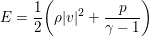
 $(E,\,v(E+{\it\gamma}p))$, where the total energy
 $$\begin{eqnarray}E=\frac{1}{2}\biggl({\it\rho}|v|^{2}+\frac{p}{{\it\gamma}-1}\biggr)\end{eqnarray}$$
serves as the convex entropy.
Theorem 2.8 (De Lellis and Székelyhidi Jr Reference De Lellis and Székelyhidi2009, Chiodaroli et al. Reference Chiodaroli, De Lellis and Kreml2015). There exist initial data  $u_{0}\in L^{1}(\mathbb{R}^{2},\mathbb{R}^{3})$ for which the two-dimensional isentropic Euler equations (2.9) have infinitely many entropy solutions.
In principle, this construction can be extended to the full compressible Euler system (1.1).
2.2 Incompressible Euler equations
We begin with a brief overview of the incompressible Euler equations (1.3). A more detailed study can be found in standard textbooks (Chorin and Marsden Reference Chorin and Marsden1993, Marchioro and Pulvirenti Reference Marchioro and Pulvirenti1994, Chemin Reference Chemin1998, Majda and Bertozzi Reference Majda and Bertozzi2002, Lions Reference Lions1996) or review papers (Constantin Reference Constantin2007, Bardos and Titi Reference Bardos and Titi2007, Reference Bardos and Titi2013) and the references therein. We first observe that the incompressible Euler equations (1.3) can be expressed as a system of  $d$-dimensional conservation laws (2.1) for the velocity field
 $u=(u_{1},\ldots ,u_{d})^{\top }:D\rightarrow \mathbb{R}^{d}$:
 $$\begin{eqnarray}\displaystyle \partial _{t}u+{\rm\nabla}_{x}\cdot f(u)=0,\quad f^{j}(u)=\mathbb{P}(u_{j}u),\quad j=1,\ldots ,d,\quad (x,t)\in D\times \mathbb{R}_{+}. & & \displaystyle \nonumber\\ \displaystyle & & \displaystyle\end{eqnarray}$$
For simplicity we focus on either the Cauchy problem,  $D=\mathbb{R}^{d}$, or the case of periodic boundary conditions over the
 $d$-dimensional torus,
 $D=\mathbb{T}^{d}$. Here,
 $\mathbb{P}:=\text{I}-{\rm\nabla}_{x}{\rm\Delta}^{-1}\text{div}_{x}$ is the Leray projection onto the space of divergence-free fields. This reflects an essential feature: the global character of the incompressible Euler fluxes.
Next, we introduce the notion of weak solutions for the incompressible Euler equations.
Definition 2.9. A divergence-free function
 $$\begin{eqnarray}u\in L^{2}([0,T];D)\cap C([0,T];L_{w}^{2}(D))\end{eqnarray}$$
is a weak solution of the incompressible Euler equations (1.3) if
 $$\begin{eqnarray}\displaystyle \int _{0}^{T}\int _{D}[u(x,t)\cdot \partial _{t}{\it\varphi}(x,t)+(u\otimes u):{\rm\nabla}_{x}{\it\varphi}]\,\text{d}x\,\text{d}t+\int _{D}u_{0}(x)\cdot {\it\varphi}(x,0)\,\text{d}x=0 & & \displaystyle \nonumber\\ \displaystyle & & \displaystyle\end{eqnarray}$$
is satisfied for every divergence-free test function  ${\it\varphi}\in C_{c}^{\infty }([0,T)\times D)$.
Note that (2.11) results from considering (1.3) in the sense of distributions, with the divergence-free condition on the test function  ${\it\varphi}$ eliminating the pressure term, thus demonstrating that it merely serves as a Lagrange multiplier to enforce the divergence-free constraint in (1.3).
Weak solutions (2.11) need not be unique, and therefore additional admissibility criteria or exclusion principles must be prescribed in order to select physically relevant solutions. One such universal admissibility criterion follows.
Definition 2.10. A weak solution  $u$ of the incompressible Euler equations (1.3) is admissible if it also satisfies the energy inequality
 $$\begin{eqnarray}\int _{D}|u(x,t)|^{2}\,\text{d}x\leq \int _{D}|u_{0}(x)|^{2}\,\text{d}x,\quad \text{for all}\;t\in [0,T].\end{eqnarray}$$
Thus, admissibility requires that kinetic energy associated with weak solutions can only dissipate in time, in complete analogy with the admissibility criterion of entropy dissipation (2.3) for weak solutions of non-linear conservation laws.
A key quantity of interest in the incompressible Euler equations is the vorticity  ${\it\omega}:=\text{curl}(u)$, which formally evolves according to
 $$\begin{eqnarray}{\it\omega}_{t}+(u\cdot {\rm\nabla}_{x}){\it\omega}=-({\it\omega}\cdot {\rm\nabla}_{x})u,\end{eqnarray}$$
where the velocity can be recovered from the vorticity,  ${\it\omega}{\rightsquigarrow}u\{{\it\omega}\}$, in terms of the streamfunction (Majda and Bertozzi Reference Majda and Bertozzi2002, Section 2). Both theoretical and numerical studies of the incompressible Euler equations (1.3) have alternated between the use of the velocity–pressure and the vorticity–streamfunction forms of the equations.
2.2.1 Classical well-posedness results
One of the earliest theoretical results about the incompressible Euler equations pertains to the following result of Lichtenstein (Reference Lichtenstein1925) on the short-time existence of classical solutions,
Theorem 2.11 (Lichtenstein Reference Lichtenstein1925).
Consider the divergence-free initial data  $u_{0}\in C^{1,{\it\alpha}}(D)$ with
 $0<{\it\alpha}<1$. Then there exists a time
 $T^{\ast }>0$ depending on
 $u_{0}$, a velocity field
 $$\begin{eqnarray}u\in C_{b}([0,T^{\ast }];C^{1,{\it\alpha}}(D))\cap C^{1}([0,T^{\ast }];C^{0,{\it\alpha}}(D))\end{eqnarray}$$
and pressure  $p\in C_{b}([0,T^{\ast }];C^{1,{\it\alpha}}(D))$, such that the pair
 $(u,p))$ solves the incompressible Euler equations (1.3) in the time interval
 $[0,T^{\ast }]$, in the classical sense.
Note that the above short-time existence result is valid for both two and three space dimensions. The question of whether one can extend this short-time existence for all times depends on the uniform bound
 $$\begin{eqnarray}\int _{0}^{T}\Vert {\rm\nabla}u(\cdot ,t)\Vert _{L^{\infty }}\,\text{d}t<\infty .\end{eqnarray}$$
In fact, certain linear combinations of the entries of  ${\rm\nabla}u$ will suffice for global regularity. The following celebrated result of Beale, Kato and Majda (Reference Beale, Kato and Majda1984) provides a sufficient condition for the interval of existence, which reflects the prominent role of the vorticity.
Theorem 2.12 (Beale et al. Reference Beale, Kato and Majda1984).
Let
 $$\begin{eqnarray}u\in C([0,T);H^{s}(D)^{3})\cap C^{1}([0,T];H^{s-1}(D)^{3}),\end{eqnarray}$$
with  $s>5/2$, be a smooth solution of the three-dimensional Euler equations (1.3) in the time interval
 $[0,T)$, and assume that
 $$\begin{eqnarray}\int _{0}^{T}\Vert \text{curl}(u(\cdot ,t))\Vert _{L^{\infty }(D)}\,\text{d}t<\infty .\end{eqnarray}$$
Then  $u$ can be uniquely extended to a smooth solution in the interval
 $[0,T+{\it\delta})$ for some
 ${\it\delta}>0$.
Thus, it is enough to control the vorticity  ${\it\omega}=\text{curl}(u)$, rather than the full gradient
 ${\rm\nabla}u$, in order to obtain global solutions. In fact, an even more refined result (Constantin, Fefferman and Majda Reference Constantin, Fefferman and Majda1996) shows that control of variations in the direction of the vorticity
 ${\it\omega}$ suffices to extend the interval of existence of regular solutions. Obtaining an
 $L^{\infty }$ bound on the three-dimensional vorticity, however, appears to be very difficult, due to possible vortex stretching driven by the right-hand side of the vorticity equation (2.13). In fact, the question of whether smooth solutions of the incompressible Euler equations blow up in finite time is still open. Numerical results (see Hou Reference Hou2008 and references therein) do suggest finite-time blow-up, particularly for problems with no-penetration boundary conditions.
The vorticity equation becomes considerably simpler in the case of two space dimensions, precisely because the vortex stretching term on the right-hand side of (2.13) vanishes. Consequently, one obtains the following global existence and uniqueness results for two-dimensional weak solutions.
Theorem 2.13 (Yudovich Reference Yudovich1963).
Consider divergence-free initial data  $u_{0}\in L^{2}(D,\mathbb{R}^{2})$ with initial vorticity
 ${\it\omega}_{0}=\text{curl}(u_{0})\in L^{\infty }(D,\mathbb{R}^{2})$. Then there exists a unique admissible weak solution of the two-dimensional incompressible Euler equations (1.3) for all times
 $t>0$.
For the mere existence of two-dimensional weak solutions, one can relax the assumption on initial regularity by considering larger classes of initial vorticities,  ${\it\omega}_{0}\in X$, which are compact in
 $H^{-1}(D)$, including
 $X=L^{p}(D)$ and the larger Morrey spaces
 $X=M^{p}(D)$ with
 $p>1$ or Lorentz space
 $X=L^{(1,2)}(D)$ (Lopes Filho, Nussenzveig and Tadmor Reference Lopes Filho, Nussenzveig and Tadmor2000). This brings us to the ‘largest’ borderline space of Radon measures
 $X={\mathcal{M}}(D)$ which, among others, realizes initial vortex sheets (DiPerna and Majda Reference DiPerna and Majda1987b). In this context, we recall the celebrated existence result of Delort.
Theorem 2.14 (Delort Reference Delort1991).
Consider the incompressible Euler equations (1.3) in two dimensions, subject to initial vorticity in the so-called Delort class of bounded measures with a distinguished (say, positive) sign,  ${\it\omega}_{0}\in X:=H^{-1}(D)\cap {\mathcal{M}}_{+}(D)$. Then there exists a weak solution
 $u$ that remains in the Delort class,
 ${\it\omega}\in L^{\infty }((0,T),X)$.
The proof is based on mollifying the initial data, resulting in the generation of a sequence of approximate (smooth) solutions to the Euler equations. The resulting vorticity will be of a definite sign as it satisfies a maximum principle. The strong compactness of the approximating sequence is based on localized  $L^{1}$ control of the vorticity and uses the fact that the vorticity is of definite sign in a crucial manner; see also Majda (Reference Majda1993) and Schochet (Reference Schochet1995). The question of uniqueness of solutions in the Delort class remains open.
2.2.2 Non-uniqueness
A recent series of remarkable results by De Lellis and Székelyhidi prove the non-uniqueness of admissible weak solutions for the incompressible Euler equations.
Theorem 2.15 (De Lellis and Székelyhidi Jr Reference De Lellis and Székelyhidi2009, Reference De Lellis and Székelyhidi2010).
Consider the incompressible Euler equations on a domain  $D\subset \mathbb{R}^{d}$ for
 $d=2,3$, and let
 $T>0$. There exist initial data
 $u_{0}\in L^{2}(D,\mathbb{R}^{2})\cap L^{\infty }(D,\mathbb{R}^{2})$ for which there are infinitely many admissible weak solutions
 $u\in L^{2}((0,T)\times D))\cap C([0,T);L_{w}^{2}(D))$. Moreover, there are infinitely many such initial data
 $u_{0}$.
The results of De Lellis and Székelyhidi significantly extend the constructions of Scheffer (Reference Scheffer1993) and Shnirelman (Reference Shnirelman2000) that led to the realization of compactly supported (in space-time) non-trivial solutions of the Euler equations. This set of infinitely many admissible weak solutions is based on an intricate construction that adds very high-frequency oscillations in an iterative procedure to construct a convergent sequence of approximate solutions of the Euler equations. The class of initial data, called wild initial data, is very rich and forms a dense subset of  $L^{2}$. In particular, vortex sheets are admissible wild initial data in this sense, although the resulting solutions no longer lie in the Delort class. Recent results by Buckmaster et al. (Reference Buckmaster, De Lellis, Isett and Székelyhidi2015) have further refined the original construction of De Lellis and Székelyhidi Jr (Reference De Lellis and Székelyhidi2009), and demonstrate the existence of infinitely many admissible Hölder-continuous weak solutions of the Euler equations.
3 Measure-valued solutions
A standard paradigm to establish the existence of weak solutions of non-linear conservation laws (including the non-local fluxes of incompressible Euler equations) is based on propagation of compactness in appropriate regularity spaces,  $\mathbf{S}_{t}:X\rightarrow X$, so that the construction of appropriate approximate solutions,
 $\{u^{{\it\varepsilon}}(\cdot ,t)=\mathbf{S}_{t}u_{0}^{{\it\varepsilon}}\}\subset X$, admits strongly converging subsequences
 $\lim _{n\rightarrow \infty }u^{{\it\varepsilon}_{n}}=u_{\infty }$ which allow the passage to a limit inside the non-linear flux,
 $\lim _{n\rightarrow \infty }f(u^{{\it\varepsilon}_{n}})=f(u_{\infty })$; see, for example, Tadmor (Reference Tadmor2012, Section 4.4). So far, such regularity spaces have been mainly limited to scalar equations and one-dimensional systems. In particular, multi-dimensional conservation laws which involve
 $d\geq 2$ spatial dimensions and three-dimensional incompressible Euler equations (or even the two-dimensional equations with ‘rough’ data), do not seem to admit known regularity space, which propagates the (compensated) compactness required to handle their respective non-linearities. Instead, we can resort to the entropy bound
 $\int _{D}{\it\eta}(u^{{\it\varepsilon}}(x,t))\,\text{d}x<\infty$ and the corresponding
 $L^{2}$ energy bound of (approximate) Euler weak solutions,
 $\Vert u^{{\it\varepsilon}}(\cdot ,t)\Vert _{L^{2}(D)}<\infty$, to conclude the existence of a subsequence
 $u^{{\it\varepsilon}_{n}}$ with a weak limit,
 $u^{{\it\varepsilon}_{n}}\stackrel{n\rightarrow \infty }{~\rightharpoonup ~}u_{\infty }$. This raises the question of the corresponding weak limit
 $f(u^{{\it\varepsilon}_{n}})$.
3.1 Young measures
In this section we present a brief but self-contained overview of the theory of Young measures. Young measures were introduced in the context of PDEs by Tartar (Reference Tartar1979) in order to represent weak* limits of  $L^{\infty }$ bounded sequences of highly oscillatory functions, in the spirit of L. C. Young (Reference Young1969). The early studies of Tartar and Murat (see Murat Reference Murat1978, Reference Murat, Giorgi, Magenes and Mosco1979, Reference Murat1981) were generalized by Schonbek (Reference Schonbek1982) and Ball (Reference Ball, Rascle, Serre and Slemrod1989) for sequences of measurable functions, and further generalization has been provided by Fjordholm et al. (Reference Fjordholm, Käppeli, Mishra and Tadmor2016a) for sequences of Young measures which do not leak mass at infinity. Here, we will review some of the material presented in the aforementioned references.
3.1.1 Probability measures
We let  ${\mathcal{M}}(\mathbb{R}^{N})$ denote the set of finite, signed Radon measures on
 $\mathbb{R}^{N}$ (Folland Reference Folland1999, Chapter 7). Let
 $C_{0}(\mathbb{R}^{N})$ be the space of continuous real-valued functions on
 $\mathbb{R}^{N}$ which vanish at infinity, equipped with the supremum norm. By the Riesz–Kakutani theorem,
 ${\mathcal{M}}(\mathbb{R}^{N})$ can be identified with the dual space of
 $C_{0}(\mathbb{R}^{N})$ via the pairing
 $$\begin{eqnarray}\langle {\it\mu},\,g\rangle =\int _{\mathbb{R}^{N}}g({\it\xi})\,\text{d}{\it\mu}({\it\xi}),\quad {\it\mu}\in {\mathcal{M}}(\mathbb{R}^{N}),~g\in C_{0}(\mathbb{R}^{N})\end{eqnarray}$$
(Folland Reference Folland1999, Section 7.3). We do not distinguish between these two equivalent definitions of  ${\mathcal{M}}$. By a slight abuse of notation, we shall sometimes write
 $$\begin{eqnarray}\langle {\it\mu},\,g({\it\xi})\rangle =\int _{\mathbb{R}^{N}}g({\it\xi})\,\text{d}{\it\mu}({\it\xi}).\end{eqnarray}$$
For instance, the first moment of  ${\it\mu}$ is
 $$\begin{eqnarray}\langle {\it\mu},\,{\it\xi}\rangle =\int _{\mathbb{R}^{N}}{\it\xi}\,\text{d}{\it\mu}({\it\xi}).\end{eqnarray}$$
The duality between  $C_{0}(\mathbb{R}^{N})$ and
 ${\mathcal{M}}(\mathbb{R}^{N})$ gives rise to a topology on
 ${\mathcal{M}}(\mathbb{R}^{N})$, that of weak* convergence. A sequence
 ${\it\mu}^{n}\in {\mathcal{M}}(\mathbb{R}^{N})$ converges weak* to
 ${\it\mu}\in {\mathcal{M}}(\mathbb{R}^{N})$ provided
 $\langle {\it\mu}^{n},\,g\rangle \rightarrow \langle {\it\mu},\,g\rangle$ for all
 $g\in C_{0}(\mathbb{R}^{N})$. (This is also called vague convergence: see Folland Reference Folland1999.)
The set of probability measures on  $\mathbb{R}^{N}$ is the subset
 $$\begin{eqnarray}{\mathcal{P}}(\mathbb{R}^{N}):=\{{\it\mu}\in {\mathcal{M}}(\mathbb{R}^{N}):{\it\mu}\geq 0,~{\it\mu}(\mathbb{R}^{N})=1\}.\end{eqnarray}$$
3.1.2 Young measures
A Young measure from  $D\subset \mathbb{R}^{k}$ to
 $\mathbb{R}^{N}$ is a function which maps
 $z\in D$ to a probability measure on
 $\mathbb{R}^{N}$. More precisely, a Young measure is a weak*-measurable map
 ${\it\nu}:D\rightarrow {\mathcal{P}}(\mathbb{R}^{N})$, meaning that:
 $$\begin{eqnarray}\text{The mapping }z\mapsto \langle {\it\nu}_{z},\,g\rangle \text{is Borel-measurable for every }g\in C_{0}(\mathbb{R}^{N}).\end{eqnarray}$$
The set of all Young measures from  $D$ into
 $\mathbb{R}^{N}$ is denoted by
 $\mathbf{Y}(D,\mathbb{R}^{N})$.
In the particular context of our discussion above, Young measures provide a complete description for bounded sequences of approximate solutions  $u_{n}=u^{{\it\varepsilon}_{n}}(x,t)$ with weak* limits
 $u_{n}(x,t)\rightharpoonup u_{\infty }(x,t)$. We ask what can be said about the corresponding weak* limits
 $f(u_{n})\rightharpoonup f_{\infty }$ for all continuous functions
 $f\in C_{0}(\mathbb{R}^{N})$. Fix
 $(x,t)\in D\times \mathbb{R}_{+}$. Since
 $f_{\infty }(x,t)$ depends linearly and positively on
 $f\in C_{0}$, it follows that there exists a Young measure
 ${\it\nu}_{x,t}$ such that
 $f_{\infty }=\langle {\it\nu}_{x,t},f({\it\xi})\rangle$.
Example 3.1. The most familiar example of Young measures are the so-called atomic Young measures associated with Borel-measurable functions  $u:D\rightarrow \mathbb{R}^{N}$:
 $$\begin{eqnarray}{\it\nu}_{z}={\it\delta}_{u(z)}.\end{eqnarray}$$
The strong convergence  $u_{n}\rightarrow u_{\infty }$ is characterized by such atomic measures:
 $$\begin{eqnarray}f(u_{n}(x,t))\rightarrow \langle {\it\delta}_{u_{\infty }(x,t)},f\rangle .\end{eqnarray}$$
This is in sharp contrast to the persistence of oscillations in weak convergence.
Example 3.2. Let  $u:D\rightarrow \mathbb{R}^{N}$ be a bounded function on the
 $2{\it\pi}$-periodic torus
 $D=\mathbb{T}^{k}$, and consider
 $u_{n}(x)=u(nx)$. Then
 $$\begin{eqnarray}u_{n}\rightharpoonup u_{\infty }=\frac{1}{(2{\it\pi})^{k}}\int _{\mathbb{T}^{k}}u(x)\,\text{d}x,\end{eqnarray}$$
and hence the corresponding weak* limits  $f_{\infty }$ differ from
 $f(u_{\infty })$,
 $$\begin{eqnarray}f(u_{n})\rightharpoonup f_{\infty }=\frac{1}{(2{\it\pi})^{k}}\int _{\mathbb{T}^{k}}f(u(x))\,\text{d}x,\end{eqnarray}$$
and are described by the Young measure
 $$\begin{eqnarray}\langle {\it\nu},f\rangle =(2{\it\pi})^{-k}\int _{\mathbb{T}^{k}}f(u(x))\,\text{d}x.\end{eqnarray}$$
The Young measure  ${\it\nu}\in \mathbf{Y}(D,\mathbb{R}^{N})$ is uniformly bounded if there is a compact set
 $K\subset \mathbb{R}^{N}$ such that
 $\text{supp}{\it\nu}_{z}\subset K$ for almost every
 $z\in D$. Note that if
 ${\it\nu}$ is atomic,
 ${\it\nu}={\it\delta}_{u}$, then
 ${\it\nu}$ is uniformly bounded if and only if
 $\Vert u\Vert _{L^{\infty }(D)}<\infty$.
Just as for the space  ${\mathcal{M}}(\mathbb{R}^{N})$, there is a natural topology on
 $\mathbf{Y}(D,\mathbb{R}^{N})$: a sequence
 ${\it\nu}^{n}\in \mathbf{Y}(D,\mathbb{R}^{N})$ converges weak* to
 ${\it\nu}\in \mathbf{Y}(D,\mathbb{R}^{N})$ if
 $\langle {\it\nu}^{n},\,g\rangle \overset{\ast }{\rightharpoonup }\langle {\it\nu},\,g\rangle$ in
 $L^{\infty }(D)$ for all
 $g\in C_{0}(\mathbb{R}^{N})$, that is,
 $$\begin{eqnarray}\int _{D}{\it\varphi}(z)\langle {\it\nu}_{z}^{n},\,g\rangle \,\text{d}z\rightarrow \int _{D}{\it\varphi}(z)\langle {\it\nu}_{z},\,g\rangle \,\text{d}z\quad \text{for all}~{\it\varphi}\in L^{1}(D).\end{eqnarray}$$
The fundamental theorem of Young measures was first introduced by Tartar for  $L^{\infty }$ bounded sequences (Tartar Reference Tartar1979) and then generalized by Schonbek (Reference Schonbek1982) and Ball (Reference Ball, Rascle, Serre and Slemrod1989) for sequences of measurable functions. A further generalization has been presented by Fjordholm et al. (Reference Fjordholm, Käppeli, Mishra and Tadmor2016a): every sequence
 ${\it\nu}^{n}\in \mathbf{Y}(D,\mathbb{R}^{N})$ which does not ‘leak mass at infinity’ (condition (3.2)) has a weak* convergent subsequence.
Theorem 3.3. Let  ${\it\nu}^{n}\in \mathbf{Y}(D,\mathbb{R}^{N})$ for
 $n\in \mathbb{N}$ be a sequence of Young measures. Then there exists a subsequence
 ${\it\nu}^{m}$ which converges weak* to a non-negative measure-valued function
 ${\it\nu}:D\rightarrow {\mathcal{M}}_{+}(\mathbb{R}^{N})$ in the sense that
(i)
 $\langle {\it\nu}_{z}^{m},\,g\rangle \overset{\ast }{\rightharpoonup }\langle {\it\nu},\,g\rangle$ in $L^{\infty }(D)$ for all $g\in C_{0}(\mathbb{R}^{N})$,



and moreover satisfies
(ii)
$\Vert {\it\nu}_{z}\Vert _{{\mathcal{M}}(\mathbb{R}^{N})}\leq 1$ for a.e. $z\in D$, and


(iii) if
$K\subset \mathbb{R}^{N}$ is closed and $\text{supp}{\it\nu}_{z}^{n}\subset K$ for a.e. $z\in D$ and $n$ large, then $\text{supp}{\it\nu}_{z}\subset K$ for a.e. $z\in D$.


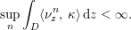
Suppose further that there exists a non-negative function  ${\it\kappa}\in C(\mathbb{R}^{N})$ with
 $\lim _{|{\it\xi}|\rightarrow \infty }{\it\kappa}({\it\xi})=\infty$ such that
 $$\begin{eqnarray}\sup _{n}\int _{D}\langle {\it\nu}_{z}^{n},\,{\it\kappa}\rangle \,\text{d}z<\infty .\end{eqnarray}$$
Then
(iv)
$\Vert {\it\nu}_{z}\Vert _{{\mathcal{M}}(\mathbb{R}^{N})}=1$ for a.e. $z\in D$,


whence  ${\it\nu}\in \mathbf{Y}(D,\mathbb{R}^{N})$.
The proof of this theorem is given in Appendix A.1 of Fjordholm et al. (Reference Fjordholm, Käppeli, Mishra and Tadmor2016a).
3.2 Measure-valued solutions for non-linear systems of conservation laws
Given the current lack of existence and uniqueness results for entropy weak solutions, as well as the lack of convergence reported in Section 1, we consider the different notion of entropy measure-valued solutions. As stated earlier, entropy measure-valued solutions for non-linear systems of conservation laws were introduced by DiPerna (Reference DiPerna1985). Here, we follow the presentation of Fjordholm et al. (Reference Fjordholm, Käppeli, Mishra and Tadmor2016a).
Definition 3.4. Let  ${\it\sigma}\in \mathbf{Y}(\mathbb{R}^{d},\,\mathbb{R}^{N})$ be uniformly bounded initial data. A family of uniformly bounded Young measures
 ${\it\nu}_{t}\in \mathbf{Y}(\mathbb{R}^{d},\,\mathbb{R}^{N})$ is a measure-valued solution (MV solution) of (2.1) with data
 ${\it\sigma}$ if
 $$\begin{eqnarray}\int _{\mathbb{R}_{+}}\int _{\mathbb{R}^{d}}(\langle {\it\nu}_{x,t},\,{\it\xi}\rangle \partial _{t}{\it\varphi}+\langle {\it\nu}_{x,t},\,f({\it\xi})\rangle \cdot {\rm\nabla}{\it\varphi})\,\text{d}x\,\text{d}t+\int _{\mathbb{R}^{d}}{\it\varphi}(x,0)\langle {\it\sigma}_{x},\,{\it\xi}\rangle \,\text{d}x=0\end{eqnarray}$$
for all  ${\it\varphi}\in C_{c}^{\infty }({\rm\Omega})$.
Note that we allow for uncertainty in the initial data by considering general initial Young measure  ${\it\sigma}$, rather than restricting attention to atomic initial data
 ${\it\sigma}={\it\delta}_{u_{0}}$.
As in the case of weak solutions, we need to impose additional admissibility criteria to enforce uniqueness of the measure-valued solution (3.3). This brings us to the following entropy inequalities.
Definition 3.5. A measure-valued solution  ${\it\nu}$ is an entropy measure-valued solution (EMV solution) of (2.1) if
 ${\it\nu}$ satisfies the following entropy inequality for all entropy pairs
 $({\it\eta},q)$:
 $$\begin{eqnarray}\displaystyle & & \displaystyle \int _{\mathbb{R}_{+}}\int _{\mathbb{R}^{d}}(\langle {\it\nu}_{x,t},\,{\it\eta}({\it\xi})\rangle \partial _{t}{\it\varphi}(x,t)+\langle {\it\nu}_{x,t},\,q({\it\xi})\rangle \cdot {\rm\nabla}_{x}{\it\varphi}(x,t))\,\text{d}x\,\text{d}t\nonumber\\ \displaystyle & & \displaystyle \qquad +\int _{\mathbb{R}^{d}}{\it\varphi}(x,0)\langle {\it\sigma}_{x},\,{\it\eta}\rangle \,\text{d}x\geq 0\end{eqnarray}$$
for all non-negative test functions  $0\leq {\it\varphi}\in C_{c}^{1}(\mathbb{R}^{d}\times \mathbb{R}_{+})$.
Remark 3.6. Note that we have assumed that the Young measure  ${\it\nu}$ in Definitions 3.4 and 3.5 is uniformly bounded. In particular, we will implicitly assume a uniform
 $L^{\infty }$ bound on any sequences that generate the entropy measure-valued solution
 ${\it\nu}$.
Remark 3.7. The formulation (3.3) imposes the initial data  ${\it\sigma}$ in a very weak manner. Roughly speaking, (3.3) requires
 $\lim _{t\rightarrow 0}\langle {\it\nu}_{x,t},\,{\it\xi}\rangle =\langle {\it\sigma}_{x},\,{\it\xi}\rangle$, that is, the barycentres (or means) of
 ${\it\nu}_{x,0}$ and
 ${\it\sigma}_{x}$ should coincide. The requirement that the barycentres of these two measures should coincide will, together with the entropy condition (3.4), imply that the measures themselves coincide only if the initial data are atomic. Extensions to more general classes of initial data are postponed to Section 9.
Among the many examples of EMVs for systems of conservation laws, we mention Kröner and Zajaczkowski (Reference Kröner and Zajaczkowski1996) for compressible Euler equations, Gwiazda (Reference Gwiazda2005) for isentropic Euler equations, Carrillo, Feireisl, Gwiazda and Swierczewska-Gwiazda (Reference Carrillo, Feireisl, Gwiazda and Swierczewska-Gwiazda2015) for ‘flocking hydrodynamics’, E and Kohn (Reference E and Kohn1991) for hyperbolic systems with linearly degenerate fields, and Málek et al. (Reference Málek, Nečas, Rokyta and Ružička1996) for non-Newtonian fluids.
The existence of EMV solutions for general multi-dimensional systems of conservation laws will be established as a proper limit of a numerical approximation procedure outlined in the next section. Uniqueness will be discussed in Section 9.
3.3 Generalized measure-valued solution for incompressible Euler equations
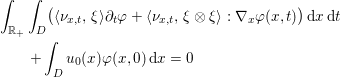
A straightforward definition of measure-valued solutions for the incompressible Euler equations (1.3) will seek divergence-free Young measures  ${\it\nu}_{t}\in \mathbf{Y}(D,\,\mathbb{R}^{d})$, which satisfy
 $$\begin{eqnarray}\displaystyle & & \displaystyle \int _{\mathbb{R}_{+}}\int _{D}(\langle {\it\nu}_{x,t},\,{\it\xi}\rangle \partial _{t}{\it\varphi}+\langle {\it\nu}_{x,t},\,{\it\xi}\otimes {\it\xi}\rangle :{\rm\nabla}_{x}{\it\varphi}(x,t))\,\text{d}x\,\text{d}t\nonumber\\ \displaystyle & & \displaystyle \qquad +\int _{D}u_{0}(x){\it\varphi}(x,0)\,\text{d}x=0\end{eqnarray}$$
for all  ${\it\varphi}\in C_{c}^{\infty }(D\times [0,\infty );\mathbb{R}^{N})$ with
 ${\rm\nabla}_{x}\cdot {\it\varphi}=0$, and
 $$\begin{eqnarray}\int _{\mathbb{R}_{+}}\int _{D}\langle {\it\nu}_{x,t},\,{\it\xi}\rangle \cdot {\rm\nabla}_{x}{\it\psi}(x,t)\,\text{d}x\,\text{d}t=0\end{eqnarray}$$
for all  ${\it\psi}\in C_{c}^{\infty }(D\times [0,\infty ))$.
The distinctive feature of (approximate) solutions to the incompressible Euler equations is their  $L^{2}$ energy bound,
 $\Vert u^{{\it\varepsilon}_{n}}(\cdot ,t)\Vert _{L^{2}(D)}<\infty$. In contrast to general systems of conservation laws, however, one should not expect for higher
 $L^{p}$ bounds,
 $p>2$, and in particular
 $u_{n}=u^{{\it\varepsilon}_{n}}$ need not be uniformly bounded in any such
 $L^{p}$ space. Consequently, Young measures describe the oscillations present in the weak limits
 $f(u_{n})$ for all functions
 $f$ with less than quadratic growth,
 $|f(u)|=o(|u|^{2})$ as
 $|u|\rightarrow \infty$, but there is a possibility of mass leakage at infinity for quadratic
 $f$. This is precisely the case one encounters with the quadratic flux in incompressible Euler equations
 $u\otimes u$ (or
 $f^{j}(u)=\mathbb{P}(u_{j}u)$ in (2.10)).
3.3.1 Concentration and generalized Young measures
We begin with the following corollary of Theorem 3.3 (see Remark 2 of Ball Reference Ball, Rascle, Serre and Slemrod1989). Let  $N\in \mathbb{N}$, fix a bounded
 $D\subset \mathbb{R}^{k}$ and let
 $\{u^{{\it\varepsilon}}\}_{{\it\varepsilon}>0}$ be an
 $L^{p}$ bounded sequence
 $u^{{\it\varepsilon}}\in L^{p}(D,\mathbb{R}^{N})$ for some
 $p>1$. Then, there is a subsequence
 $u^{{\it\varepsilon}_{n}}$ and a Young measure
 ${\it\nu}\in \mathbf{Y}(D,\mathbb{R}^{N})$ such that
 $$\begin{eqnarray}g(u^{{\it\varepsilon}_{n}})\overset{\ast }{\rightharpoonup }\langle {\it\nu},\,g\rangle \quad \text{in }~~{\mathcal{M}}(D)\text{ as }n\rightarrow \infty\end{eqnarray}$$
for all  $g$ with growth strictly slower than
 $|u|^{p}$, namely,
 $$\begin{eqnarray}\int _{D}{\it\varphi}(x)g(u^{{\it\varepsilon}_{n}}(x))\,\text{d}x=\int _{D}{\it\varphi}(x)\langle {\it\nu}_{x},\,g\rangle \,\text{d}x\end{eqnarray}$$
for all  $g$ of the form
 $g(u)=(1+|u|^{p})g_{0}(u)$ with
 $g_{0}\in C_{0}(\mathbb{R}^{N})$. The above result does not address the question of convergence of
 $g(u^{{\it\varepsilon}})$ for
 $g$ with growth equal to
 $|u|^{p}$,
 $$\begin{eqnarray}\exists g_{b}\in C_{b}(\mathbb{R}^{N})\quad \text{such that}\quad g(u)=(1+|u|^{p})g_{b}(u)\quad \text{for all}~u\in \mathbb{R}^{N}.\end{eqnarray}$$
What can go wrong in such cases is that  $u^{{\it\varepsilon}}$ can concentrate mass at a rate of
 $|u^{{\it\varepsilon}}|^{p}$ as
 ${\it\varepsilon}\rightarrow 0$, so that there exist sets
 $K_{{\it\varepsilon}}\subset D$ of Lebesgue measure
 $|K_{{\it\varepsilon}}|\rightarrow 0$ with
 $$\begin{eqnarray}\int _{K_{{\it\varepsilon}}}|u^{{\it\varepsilon}}(x)|^{p}\,\text{d}x\geq c\quad \text{for all}~{\it\varepsilon}>0\end{eqnarray}$$
for some  $c>0$, while for any
 $q<p$ we have
 $$\begin{eqnarray}\displaystyle \int _{K_{{\it\varepsilon}}}|u^{{\it\varepsilon}}(x)|^{q}\,\text{d}x\leq \biggl(\int _{K_{{\it\varepsilon}}}|u^{{\it\varepsilon}}(x)|^{p}\,\text{d}x\biggr)^{q/p}|K_{{\it\varepsilon}}|^{p/(p-q)}\leq C|K_{{\it\varepsilon}}|^{p/(p-q)}\rightarrow 0 & & \displaystyle \nonumber\\ \displaystyle & & \displaystyle\end{eqnarray}$$
as  ${\it\varepsilon}\rightarrow 0$. Thus, the concentration of mass is not detected by functions behaving like
 $|u|^{q}$ for
 $q<p$. This scenario may be encountered in the setting of systems of conservation laws (2.1) (and the incompressible Euler equations (1.3)), with a generic
 $L^{2}$ bound
 $\Vert u(\cdot ,t)\Vert _{L^{2}(\mathbb{R}^{d})}\leq C$. We can view
 $\{u(\cdot ,t)\}_{t\geq 0}$ as a sequence of functions indexed by
 $t$, such that
 $u(\cdot ,t)$ might exhibit concentration of mass at a rate of
 $|u|^{2}$ as
 $t\rightarrow T$ for some
 $T>0$, in the sense that there are spatial subsets
 $K_{t}\subset \mathbb{R}^{d}$ of Lebesgue measure
 $|K_{t}|\rightarrow 0$ as
 $t\rightarrow T$ such that (cf. (3.7a))
 $$\begin{eqnarray}\int _{K_{t}}|u(x,t)|^{2}\,\text{d}x\geq c>0\quad \text{for all}~t<T.\end{eqnarray}$$
Example 3.8. Let  $T=1$ and
 $$\begin{eqnarray}u(x,t):=\left\{\begin{array}{@{}ll@{}}\displaystyle \frac{1}{\sqrt{1-t}}\quad & \text{if }|x|<1-t,\\ 0\quad & \text{else},\end{array}\right.\quad \text{for }0\leq t\leq 1.\end{eqnarray}$$
Then, for  $t<1$,
 $$\begin{eqnarray}\int _{\mathbb{R}}|u(x,t)|^{2}\,\text{d}x=\int _{-(1-t)}^{1-t}|u(x,t)|^{2}\,\text{d}x\equiv 2.\end{eqnarray}$$
Hence, if  $K_{t}:=[-(1-t),1-t]$ then (3.7a) holds with
 $p=2$,
 $c=2$, while
 $$\begin{eqnarray}\int _{\mathbb{R}}|u(x,t)|^{q}\,\text{d}x=2(1-t)^{1-q/2}\rightarrow \left\{\begin{array}{@{}ll@{}}0\quad & \text{if }q<2,\\ \infty \quad & \text{if }q>2,\end{array}\right.\quad \text{as }t\rightarrow 1.\end{eqnarray}$$
Since  $u(x,t)\rightarrow 0$ as
 $t\rightarrow 1$ for every
 $x\in \mathbb{R}$, the Young measure associated with the sequence
 $\{u(\cdot ,t)\}_{t<1}$ is simply
 ${\it\nu}_{x}\equiv {\it\delta}_{0}$, but clearly
 $\int _{\mathbb{R}}|u(x,t)|^{2}\,\text{d}x$ does not converge to
 $\int _{\mathbb{R}}\langle {\it\nu}_{x},\,|{\it\xi}|^{2}\rangle \,\text{d}x=0$.
Given the above discussion, we need a framework to describe the limits of functions (or, more generally, Young measures) that exhibit both oscillations as well as concentration. General frameworks which provide a detailed description of both oscillations and concentrations include Tartar’s  $H$-measures (Tartar Reference Tartar1990) and Gérard’s microlocal defect measures (Gérard Reference Gérard1991). Here we use the notion of generalized Young measures, introduced by DiPerna and Majda (Reference DiPerna and Majda1987a) precisely to address the question of concentration in the context of the incompressible Euler equations. We follow the general framework of Alibert and Bouchitté (Reference Alibert and Bouchitté1997).
Definition 3.9 (Alibert and Bouchitté Reference Alibert and Bouchitté1997, Székelyhidi Jr and Wiedemann Reference Székelyhidi and Wiedemann2012). Let  $D$ be an open set in Euclidean space, and let
 $S^{N-1}$ denote the unit sphere in
 $\mathbb{R}^{N}$. A generalized Young measure on
 $D$ is a triple
 $({\it\nu},{\it\lambda},{\it\nu}^{\infty })$ consisting of a Young measure
 ${\it\nu}:D\rightarrow {\mathcal{P}}(\mathbb{R}^{N})$, a measure
 ${\it\lambda}\in {\mathcal{M}}_{+}(D)$ which is singular with respect to Lebesgue measure, and a weak*-measurable map
 ${\it\nu}^{\infty }:D\rightarrow {\mathcal{P}}(S^{N-1})$ defined for
 ${\it\lambda}$-a.e.
 $z\in D$. The objects
 ${\it\nu}$,
 ${\it\lambda}$ and
 ${\it\nu}^{\infty }$ are called the oscillation measure, the concentration measure and the concentration-angle measure, respectively.
3.3.2 Convergence of $L^{1}$ bounded sequence of functions

For the sake of notational simplicity we will consider sequences of functions which are bounded in  $L^{1}(D)$, and study functions
 $g$ with at most linear growth, that is, (3.6) with
 $p=1$. The general setting is considered in Section 3.3.3. Here and below,
 $D$ denotes an arbitrary open set in Euclidean space, and
 ${\mathcal{L}}$ will denote Lebesgue measure on
 $D$.
We let  $B:=\{z\in \mathbb{R}^{N}:|z|<1\}$ denote the open unit ball in
 $\mathbb{R}^{N}$, and
 $\bar{B}$ its closure. Let
 $C(E)$ be the space of continuous, real-valued functions on
 $E$. We can identify
 $C(D\times \mathbb{R}^{N})$ with
 $C(D\times B)$ via
 $$\begin{eqnarray}\widetilde{g}(x,z):=g\biggl(x,\frac{z}{1-|z|}\biggr)(1-|z|),\quad (x,z)\in D\times B.\end{eqnarray}$$
Note that if  $g$ has linear growth (i.e., it satisfies (3.6) with
 $p=1$) then
 $\widetilde{g}\in C_{b}(D\times B)$. We let
 $C_{1}$ denote the set of those
 $g\in C(D\times B)$ with linear growth for which
 $\widetilde{g}$ can be extended to a continuous function on
 $D\times \bar{B}$:
 $$\begin{eqnarray}C_{1}:=\{g\in C(D\times \mathbb{R}^{N}):\exists ~{\rm\Phi}\in C(D\times \bar{B})\text{ such that }{\rm\Phi}\big|_{D\times B}=\widetilde{g}\}.\end{eqnarray}$$
By a slight abuse of notation, we denote this unique extension by  $\widetilde{g}\in C(D\times \bar{B})$, for
 $g\in C_{1}$. The recession function of
 $g$ is defined by
 $g^{\infty }:=\widetilde{g}\big|_{D\times S^{N-1}}$, the restriction of
 $\widetilde{g}$ to the unit sphere
 $S^{N-1}=\partial B$. Thus, for
 $g\in C_{1}$,
 $$\begin{eqnarray}\widetilde{g}(x,z)=\left\{\begin{array}{@{}ll@{}}\displaystyle g\biggl(x,\frac{z}{1-|z|}\biggr)(1-|z|)\quad & \text{if }z\in B,\\ g^{\infty }(x,z)\quad & \text{if }x\in S^{N-1}.\end{array}\right.\end{eqnarray}$$
Conversely, for  ${\rm\Phi}\in C(D\times \bar{B})$, we define the inverse operation
 $$\begin{eqnarray}\widehat{{\rm\Phi}}(x,u):={\rm\Phi}\biggl(x,\frac{u}{1+|u|}\biggr)(1+|u|),\quad (x,u)\in D\times \mathbb{R}^{N}.\end{eqnarray}$$
Then  $\widehat{{\rm\Phi}}\in C_{1}$, and in particular,
 $\widehat{\widetilde{g}}=g$ for all
 $g\in C_{1}$. Clearly,
 $C_{0}(D\times \mathbb{R}^{N})\subset C_{1}$, and if
 $g\in C_{0}(D\times \mathbb{R}^{N})$ then
 $g^{\infty }\equiv 0$.
Theorem 3.10 (Alibert and Bouchitté Reference Alibert and Bouchitté1997).
Let  $\{u^{n}\}_{n}\!\subset \!L^{1}(D,\mathbb{R}^{N})$ be a sequence of functions such that
 $$\begin{eqnarray}\int _{D}|u^{n}(x)|\,\text{d}x\leq C\quad \text{for all}~n.\end{eqnarray}$$
Then there exists a subsequence, still denoted  $\{u^{n}\}_{n}$, and a generalized Young measure
 $({\it\nu},{\it\lambda},{\it\nu}^{\infty })$ such that
 $$\begin{eqnarray}g(u^{n}){\mathcal{L}}\overset{\ast }{\rightharpoonup }\langle {\it\nu},\,g\rangle {\mathcal{L}}+\langle {\it\nu}^{\infty },\,g^{\infty }\rangle {\it\lambda}\quad \text{in }{\mathcal{M}}(D)\end{eqnarray}$$
for all  $g\in C_{1}$, that is,
 $$\begin{eqnarray}\displaystyle & & \displaystyle \int _{D}{\it\varphi}(x)g(x,u^{n})\,\text{d}x\rightarrow \nonumber\\ \displaystyle & & \displaystyle \qquad \int _{D}{\it\varphi}(x)\int _{\mathbb{R}^{N}}g(x,u)\,\text{d}{\it\nu}_{x}(u)\,\text{d}x+\int _{D}{\it\varphi}(x)\int _{S^{N-1}}g^{\infty }(x,z)\,\text{d}{\it\nu}_{x}^{\infty }(z)\,\text{d}{\it\lambda}(x)\nonumber\end{eqnarray}$$
for all  ${\it\varphi}\in C_{0}(D)$.
3.3.3 Convergence of $L^{p}$ bounded functions

Although the framework described in the previous section only deals with sequences of Young measures (or, as a particular case, functions) that are  $L^{1}$ bounded, this theory may be easily extended to
 $L^{p}$ bounds as follows.
Fix  $p\geq 1$. The
 $L^{p}$ recession function
 $g^{\infty }$ of a function
 $g\in C(D\times \mathbb{R}^{N})$ is defined as
 $$\begin{eqnarray}g^{\infty }(x,z):=\lim _{s\rightarrow \infty }\frac{g(x,sz)}{s^{p}},\quad z\in S^{N-1}\end{eqnarray}$$
(provided the limit exists). We define  $C_{p}$ as
 $$\begin{eqnarray}C_{p}:=\{g\in C(D\times \mathbb{R}^{N}):g(x,u)=g_{1}(x,u)|u|^{p-1}\text{ for some }g_{1}\in C_{1}\}.\end{eqnarray}$$
Corollary 3.11. Let  $\{u^{n}\}_{n}$ be a sequence of functions such that
 $$\begin{eqnarray}\int _{D}|u^{n}|^{p}\,\text{d}x\leq C\quad \text{for all}~n\end{eqnarray}$$
for some  $p\geq 1$. Then there exists a subsequence, still denoted
 $\{u^{n}\}_{n}$, and a generalized Young measure
 $({\it\nu},{\it\lambda},{\it\nu}^{\infty })$ such that
 $$\begin{eqnarray}g(u^{n}){\mathcal{L}}\overset{\ast }{\rightharpoonup }\langle {\it\nu},\,g\rangle {\mathcal{L}}+\langle {\it\nu}^{\infty },\,g^{\infty }\rangle {\it\lambda}\quad \text{in }{\mathcal{M}}(D)\end{eqnarray}$$
for all  $g\in C_{p}$.
Proof. Define  $\widetilde{u}^{n}:=u^{n}|u^{n}|^{p-1}$. Then
 $\widetilde{u}^{n}$ satisfies the integrability condition (3.10). Let
 $(\widetilde{{\it\nu}},\widetilde{{\it\lambda}},\widetilde{{\it\nu}^{\infty }})$ be the generalized Young measure associated with
 $u^{n}$. For a fixed
 $g\in C_{p}$, let
 $\widetilde{g}(x,\widetilde{u}):=g(x,\widetilde{u}|\widetilde{u}|^{1/p-1})$, and define
 $({\it\nu},{\it\lambda},{\it\nu}^{\infty })$ as
 $$\begin{eqnarray}\langle {\it\nu}_{x},\,g\rangle :=\int _{\mathbb{R}^{N}}\widetilde{g}(x,\widetilde{{\it\xi}})\,\text{d}\widetilde{{\it\nu}}_{x}(\widetilde{{\it\xi}}),\quad {\it\nu}^{\infty }:=\widetilde{{\it\nu}}^{\infty },\quad {\it\lambda}:=\widetilde{{\it\lambda}}\end{eqnarray}$$
for  $g\in C_{0}(\mathbb{R}^{N})$. Clearly, both
 ${\it\nu}$ and
 ${\it\nu}^{\infty }$ are Young measures. We conclude that
 $$\begin{eqnarray}g(x,u^{n})=\widetilde{g}(x,\widetilde{u}^{n})\overset{\ast }{\rightharpoonup }\langle \widetilde{{\it\nu}},\,\widetilde{g}\rangle {\mathcal{L}}+\langle \widetilde{{\it\nu}}^{\infty },\,\widetilde{g}^{\infty }\rangle \widetilde{{\it\lambda}}=\langle {\it\nu},\,g\rangle {\mathcal{L}}+\langle {\it\nu}^{\infty },\,g^{\infty }\rangle {\it\lambda}.\square\end{eqnarray}$$
Theorem 3.10 and Corollary 3.11 can be easily generalized to sequences of ‘ $L^{p}$ bounded’ Young measures
 ${\it\nu}^{n}:D\rightarrow {\mathcal{P}}(\mathbb{R}^{N})$, such that
 $$\begin{eqnarray}\langle {\it\nu}_{x}^{n},\,|{\it\xi}|^{p}\rangle =\int _{\mathbb{ R}^{N}}|{\it\xi}|^{p}\,\text{d}{\it\nu}_{x}^{n}({\it\xi})<\infty .\end{eqnarray}$$
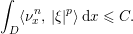
Theorem 3.12. Let  $p\geq 1$ and let
 $\{{\it\nu}^{n}\}_{n}$ be a sequence of Young measures such that
 $$\begin{eqnarray}\int _{D}\langle {\it\nu}_{x}^{n},\,|{\it\xi}|^{p}\rangle \,\text{d}x\leq C.\end{eqnarray}$$
Then there exists a subsequence, still denoted  $\{{\it\nu}^{n}\}_{n}$, and a generalized Young measure
 $({\it\nu},{\it\lambda},{\it\nu}^{\infty })$ such that
 $$\begin{eqnarray}\langle {\it\nu}^{n},\,g\rangle {\mathcal{L}}\overset{\ast }{\rightharpoonup }\langle {\it\nu},\,g\rangle {\mathcal{L}}+\langle {\it\nu}^{\infty },\,g^{\infty }\rangle m\quad \text{in }{\mathcal{M}}(D)\end{eqnarray}$$
for all  $g\in C_{p}$, that is,
 $$\begin{eqnarray}\displaystyle & & \displaystyle \int _{D}{\it\varphi}(x)\int _{\mathbb{R}^{N}}g(x,{\it\xi})\,\text{d}{\it\nu}_{x}^{n}({\it\xi})\,\text{d}x\rightarrow \nonumber\\ \displaystyle & & \displaystyle \qquad \int _{D}{\it\varphi}(x)\int _{\mathbb{R}^{N}}g(x,{\it\xi})\,\text{d}{\it\nu}_{x}({\it\xi})\,\text{d}x+\int _{D}{\it\varphi}(x)\int _{S^{N-1}}g^{\infty }(x,z)\,\text{d}{\it\nu}_{x}^{\infty }(z)\,\text{d}{\it\lambda}(x)\nonumber\end{eqnarray}$$
for all  ${\it\varphi}\in C_{0}(D)$.
The proof of this theorem is presented in the Appendix.
3.3.4 Generalized measure-valued solutions of incompressible Euler equations
Equipped with above notation, we define generalized measure-valued solutions of the incompressible Euler equations as follows.
Definition 3.13. A family of generalized Young measures  $({\it\nu}_{t},{\it\lambda}_{t},{\it\nu}_{t}^{\infty })$ on
 $D$, parametrized by
 $t\geq 0$, is a measure-valued solution of the incompressible Euler equations (1.3) with initial data
 $u_{0}$ if it satisfies
 $$\begin{eqnarray}\displaystyle & & \displaystyle \int _{\mathbb{R}_{+}}\int _{D}\langle {\it\nu}_{x,t},\,{\it\xi}\rangle \partial _{t}{\it\varphi}(x,t)+\langle {\it\nu}_{x,t},\,{\it\xi}\otimes {\it\xi}\rangle :{\rm\nabla}_{x}{\it\varphi}(x,t)\,\text{d}x\,\text{d}t\nonumber\\ \displaystyle & & \displaystyle \qquad +\int _{\mathbb{R}_{+}}\int _{D}\langle {\it\nu}_{x,t}^{\infty },\,{\it\theta}\otimes {\it\theta}\rangle :{\rm\nabla}_{x}{\it\varphi}(x,t)\,\text{d}{\it\lambda}_{t}(x)\,\text{d}t+\int _{D}u_{0}(x){\it\varphi}(x,0)\,\text{d}x=0\end{eqnarray}$$
for all  ${\it\varphi}\in C_{c}^{\infty }(D\times \mathbb{R}_{+};\,\mathbb{R}^{N})$ with
 ${\rm\nabla}_{x}\cdot {\it\varphi}=0$, and
 $$\begin{eqnarray}\displaystyle \int _{0}^{\infty }\int _{D}\langle {\it\nu}_{x,t},\,{\it\xi}\rangle \cdot {\rm\nabla}_{x}{\it\psi}(x,t)\,\text{d}x\,\text{d}t=0 & & \displaystyle\end{eqnarray}$$
for all  ${\it\psi}\in C_{c}^{\infty }(D\times [0,\infty ))$.
Note that if the Young measure is atomic, that is,  ${\it\nu}_{x,t}={\it\delta}_{u(x,t)}$ and
 ${\it\lambda}\equiv 0$, then the definition of measure-valued solutions reduces to the standard notion of weak solutions (2.11).
The global existence of measure-valued solutions was shown by DiPerna and Majda (Reference DiPerna and Majda1987a).
Theorem 3.14 (DiPerna and Majda Reference DiPerna and Majda1987a).
Let  $D\subset \mathbb{R}^{d}$ for
 $d=2,3$, and consider the incompressible Euler equations (1.3) subject to initial data
 $u_{0}\in L^{2}(D)$. Then they admit a measure-valued solution so that (3.16) holds. Moreover, this measure-valued solution is the weak* limit (up to a subsequence) of a sequence of Leray–Hopf weak solutions of the incompressible Navier–Stokes equations with vanishing viscosity.
Thus, measure-valued solutions are a framework of solutions for which global existence is guaranteed. Furthermore, they do characterize the (physically relevant) zero-viscosity limit of the Navier–Stokes equations, thus approximating very high Reynolds number flows. On the other hand, the question of uniqueness of measure-valued solutions is more delicate. At the very least, we require the following notion of admissibility.
Definition 3.15. A measure-valued solution  $({\it\nu}_{t},{\it\lambda}_{t},{\it\nu}_{t}^{\infty })$ with initial data
 $u_{0}\in L^{2}(D,\mathbb{R}^{2})$ is called admissible if
 $$\begin{eqnarray}\int _{D}\langle {\it\nu}_{x,t},|{\it\xi}|^{2}\rangle \,\text{d}x+{\it\lambda}_{t}(D)\leq \int _{D}|u_{0}(x)|^{2}\,\text{d}x\end{eqnarray}$$
for almost all  $t\in [0,\infty )$.
Remark 3.16. The  $L^{2}$ recession function of the function
 $g({\it\xi})=|{\it\xi}|^{2}$ is
 $g^{\infty }\equiv 1$ (see Section 3.3.3), so the ‘squared
 $L^{2}$ norm’ of
 $({\it\nu}_{t},{\it\lambda}_{t},{\it\nu}_{t}^{\infty })$ is
 $$\begin{eqnarray}\int _{D}\langle {\it\nu}_{x,t},\,g\rangle \,\text{d}x+\int _{D}\langle {\it\nu}_{x,t}^{\infty },\,g^{\infty }\rangle \,\text{d}{\it\lambda}_{t}(x)=\int _{D}\langle {\it\nu}_{x,t},\,|{\it\xi}|^{2}\rangle \,\text{d}x+{\it\lambda}_{t}(D).\end{eqnarray}$$
Hence the left-hand side of (3.17).
Given the fact that weak solutions are also measure-valued solutions (in particular, atomic MV solutions), Theorem 2.15 implies that there are also infinitely many admissible measure-valued solutions of the incompressible Euler equations. However, one can prove the following MV-strong uniqueness result.
Theorem 3.17 (Brenier, De Lellis and Székelyhidi Jr Reference Brenier, De Lellis and Székelyhidi2011). Let  $u\in C([0,T];L^{2}(D,\mathbb{R}^{d}))$ (with
 $d=2$ or 3) be a weak solution of (1.3) with
 $$\begin{eqnarray}\int _{0}^{T}\Vert {\rm\nabla}u+{\rm\nabla}u^{\top }\Vert _{L^{\infty }}\,\text{d}t<\infty ,\end{eqnarray}$$
and let  $({\it\nu}_{t},{\it\lambda}_{t},{\it\nu}_{t}^{\infty })$ be an admissible measure-valued solution with initial data
 ${\it\nu}_{0}={\it\delta}_{u_{0}(x)}$ and
 $u_{0}\in L^{2}(D)$. Then
 ${\it\nu}_{x,t}={\it\delta}_{u(x,t)}$ and
 ${\it\lambda}=0$, that is,
 $v$ is the unique admissible MV solution.
Thus, admissible measure-valued solutions of the Euler equations coincide with classical solutions when they exist. The question of uniqueness (stability) of admissible measure-valued solutions is further investigated in Section 9.
3.4 Generalized measure-valued solutions for systems of conservation laws
It is possible to extend the notion of generalized entropy measure-valued solutions for systems of conservation laws (2.1) without an  $L^{\infty }$ bound. The main feature here is that the
 $L^{p}$ growth of the flux
 $f$,
 $$\begin{eqnarray}|f(u)|\leq C(1+|u|^{p})\quad \text{for all}~u\in \mathbb{R}^{N},\end{eqnarray}$$
is controlled by an  $L^{p}$ growth of an entropy bound. To this end, we assume that (2.1) is equipped with an entropy function
 ${\it\eta}(u)$ with ‘
 $L^{p}$ growth’ for some
 $p>1$, in the sense that there exist
 $c_{1},c_{2}>0$ such that
 $$\begin{eqnarray}c_{1}|u|^{p}\leq {\it\eta}(u)\leq c_{2}|u|^{p}\quad \text{for all}~u\in \mathbb{R}^{N}.\end{eqnarray}$$
The entropy condition (2.3) then leads to a uniform  $L^{p}$ bound
 $$\begin{eqnarray}\text{ess}~\text{sup}_{t\in \mathbb{R}_{+}}\Vert u(t)\Vert _{L^{p}(\mathbb{R}^{d})}\leq C.\end{eqnarray}$$
The  $L^{p}$ boundedness of
 $u$ then implies that
 $f(u)$ is integrable. Using the machinery of generalized Young measures we proceed with the following notion of generalized entropy measure-valued solution subject to initial Young measure data
 ${\it\sigma}$.
Definition 3.18. Let  ${\it\sigma}\in \mathbf{Y}(\mathbb{R}^{d},\mathbb{R}^{N})$ be the initial data. A generalized Young measure
 $({\it\nu}_{t},{\it\lambda}_{t},{\it\nu}_{t}^{\infty })$ on
 $\mathbb{R}^{d}$, parametrized by
 $t\in \mathbb{R}_{+}$, is a measure-valued solution of (2.1) with data
 ${\it\sigma}$ if
 $$\begin{eqnarray}\displaystyle & & \displaystyle \int _{\mathbb{R}_{+}}\biggl[\int _{\mathbb{R}^{d}}\Big(\langle {\it\nu}_{x,t},\,{\it\xi}\rangle \partial _{t}{\it\varphi}+\langle {\it\nu}_{x,t},\,f\rangle \cdot {\rm\nabla}{\it\varphi}\Big)\,\text{d}x+\int _{\mathbb{R}^{d}}\langle {\it\nu}_{x,t}^{\infty },\,f^{\infty }\rangle \,\text{d}{\it\lambda}_{t}\biggr]\,\text{d}t\nonumber\\ \displaystyle & & \displaystyle \qquad +\int _{\mathbb{R}^{d}}{\it\varphi}(x,0)\langle {\it\sigma}_{x},\,{\it\xi}\rangle \,\text{d}x=0\end{eqnarray}$$
for all  ${\it\varphi}\in C_{c}^{\infty }({\rm\Omega})$. (Here,
 $f^{\infty }$ is the
 $L^{p}$ recession function of the flux function
 $f$.)
There are infinitely many generalized measure-valued solutions of the compressible Euler equations. Additional admissibility criteria are required to rule out non-uniqueness. We begin with the following weak–strong uniqueness result for the isentropic Euler equations (2.9).
Theorem 3.19 (Gwiazda et al. Reference Gwiazda, Swierczewska-Gwiazda and Wiedemann2015).
Let  $({\it\rho},v)\in W^{1,\infty }\times C^{1}([0,T]\times \mathbb{T}^{d})$ be a classical solution of the isentropic Euler equations (2.9) with initial data
 $0<c<{\it\rho}_{0}\in L^{{\it\gamma}}(\mathbb{T}^{d})$,
 ${\it\rho}_{0}|v_{0}|^{2}\in L^{1}(\mathbb{T}^{d})$. Let
 $({\it\nu}_{t},{\it\lambda}_{t},{\it\nu}_{t}^{\infty })$ be a generalized measure-valued solution subject to the same initial data. Then
 ${\it\nu}_{x,t}={\it\delta}_{{\it\rho},\sqrt{{\it\rho}}v(x,t)}$ and
 $({\it\lambda}_{t},{\it\nu}_{t}^{\infty })\equiv 0$, that is,
 ${\it\nu}$ is the unique admissible generalized measure-valued solution. Thus, admissible measure-valued solutions of the Euler equations coincide with strong solutions as long as the latter exist.
As in the case of weak solutions, we need to impose some additional admissibility criteria to enforce uniqueness of the measure-valued solution (3.21). DiPerna (Reference DiPerna1985) (see also Fjordholm et al. Reference Fjordholm, Käppeli, Mishra and Tadmor2016a) imposes a suitable variant of the entropy condition (2.3). However, as we are working with generalized Young measures, it may not be possible to interpret the entropy flux  $q(u)$, since
 $q$ will in general have a speed of growth larger than
 $|u|^{p}$ as
 $|u|\rightarrow \infty$. Consequently, we work with the notion of dissipative measure-valued solutions, as proposed by Demoulini et al. (Reference Demoulini, Stuart and Tzavaras2012).
Definition 3.20. A measure-valued solution of (2.1) is a dissipative MV solution if
 $$\begin{eqnarray}\displaystyle & & \displaystyle \int _{\mathbb{R}_{+}}\biggl(\int _{\mathbb{R}^{d}}\langle {\it\nu}_{x,t},\,{\it\eta}\rangle \,\text{d}x+\int _{\mathbb{R}^{d}}\langle {\it\nu}_{x,t}^{\infty },\,{\it\eta}^{\infty }\rangle \,\text{d}{\it\lambda}_{t}(x)\biggr)\frac{\text{d}{\it\phi}}{\text{d}t}(t)\,\text{d}t\nonumber\\ \displaystyle & & \displaystyle \qquad +\int _{\mathbb{R}^{d}}\langle {\it\sigma}_{x},\,{\it\eta}\rangle {\it\phi}(0)\,\text{d}x\geq 0\end{eqnarray}$$
for all  $0\leq {\it\phi}\in C_{c}^{\infty }(\mathbb{R}_{+})$.
Note that, formally speaking, the entropy condition (3.22) corresponds to setting  ${\it\varphi}(x,t)={\it\phi}(t)$ in (2.3). We observe that the assumption (3.22) implies that a dissipative measure-valued solution satisfies a generalization of the admissibility condition for the incompressible Euler equations (Definition 3.15 with
 $p=2$).
The existence of dissipative measure-valued solutions for generic multi-dimensional systems of conservation laws (with a strictly convex entropy) will be obtained in the next section by constructing a dissipative measure-valued solution using a numerical approximation procedure. Uniqueness will be discussed in Section 9.
PART TWO
Numerical approximation
In Section 4 we will review a novel algorithm to numerically approximate admissible measure-valued solutions, introduced by Fjordholm et al. (Reference Fjordholm, Käppeli, Mishra and Tadmor2016a) in the context of systems of conservation laws. In Sections 5 and 6 we discuss the application of this algorithm to systems of conservation laws and the incompressible Euler equations, respectively. We end Part 3.20 by presenting several numerical experiments in Sections 7 and 8.
4 The FKMT algorithm for approximating measure-valued solutions
In Fjordholm, Käppeli, Mishra and Tadmor (Reference Fjordholm, Käppeli, Mishra and Tadmor2016a) we propose a novel algorithm to compute measure-valued solutions. The algorithm can be cast into a more generic form that allows it to be employed for approximating measure-valued solutions for any class of PDEs.
4.1 General initial data
Algorithm 4.1. Let the initial data for an underlying time-dependent PDE be given as a Young measure  ${\it\sigma}\in \mathbf{Y}(D,\mathbb{R}^{N})$.
- Step 1:
Let
$u_{0}:{\rm\Omega}\mapsto L^{p}(\mathbb{R}^{d})$ be a random field on a probability space $({\rm\Omega},{\mathcal{X}},\mathsf{P})$ with law ${\it\sigma}$, that is, ${\it\sigma}(E)=\mathsf{P}(u_{0}({\it\omega})\in E)$.- Step 2:
Evolve the initial random field by applying a suitable numerical scheme, with solution map
$\mathbf{S}_{t}^{{\rm\Delta}}$, to the initial data $u_{0}({\it\omega})$ for every ${\it\omega}\in {\rm\Omega}$, obtaining an approximate random field $u^{{\rm\Delta}}({\it\omega};\cdot ,t):=\mathbf{S}_{t}^{{\rm\Delta}}u_{0}({\it\omega};\cdot )$.- Step 3:
Define the approximate measure-valued solution
${\it\nu}^{{\rm\Delta}}$ as the law of $u^{{\rm\Delta}}$ with respect to $\mathsf{P}$, that is, for all Borel sets $E\subset \mathbb{R}^{N}$, $$\begin{eqnarray}{\it\nu}_{x,t}^{{\rm\Delta}}(E)=\mathsf{\mathsf{P}}(u({\it\omega};x,t)\in E).\end{eqnarray}$$










It was shown in Fjordholm et al. (Reference Fjordholm, Käppeli, Mishra and Tadmor2016a, Appendix A.3.1) that  ${\it\nu}^{{\rm\Delta}}$ are indeed Young measures. The existence of a random field
 $u_{0}$ with a given law
 ${\it\sigma}$, as required in Step 1, is guaranteed by the following result.
Lemma 4.2 (Proposition A.3 in Fjordholm et al. Reference Fjordholm, Käppeli, Mishra and Tadmor2016a). We let  ${\it\sigma}\in \mathbf{Y}(D,\,\mathbb{R}^{N})$ be a Young measure on
 $D\subset \mathbb{R}^{d}$. Then there exists a random field
 $u_{0}:{\rm\Omega}\times D\rightarrow \mathbb{R}^{N}$ on a probability space
 $({\rm\Omega},{\mathcal{X}},\mathsf{P})$ such that
 $u$ has law
 ${\it\sigma}$, in the sense that
 $$\begin{eqnarray}{\it\sigma}_{x}(E)=\mathsf{P}(u_{0}({\it\omega};x)\in E)\end{eqnarray}$$
for any Borel set  $E\subset \mathbb{R}^{N}$ and almost every
 $x\in D$.
Note that we have not specified the ‘suitable numerical scheme’  $\mathbf{S}_{t}^{{\rm\Delta}}$. Instead, Algorithm 4.1 serves as a general recipe for approximating measure-valued solutions for a large class of problems. Examples of suitable solution operators
 $\mathbf{S}_{t}^{{\rm\Delta}}$, mentioned in Step 2, will be provided in subsequent sections. Depending on the appropriate choice of
 $\mathbf{S}_{t}^{{\rm\Delta}}$, we will show that the computed measure-valued solution
 ${\it\nu}^{{\rm\Delta}}$ converges to an (admissible) measure-valued solution as the discretization parameter
 ${\rm\Delta}$ is refined.
4.2 Atomic initial data
As mentioned in Section 2, measure-valued solutions will not be unique in general, when the initial Young measure  ${\it\sigma}$ is non-atomic – that is, when
 ${\it\sigma}$ cannot be written as
 ${\it\sigma}_{x}={\it\delta}_{u_{0}(x)}$ for some function
 $u_{0}$. This non-uniqueness holds even for scalar conservation laws; see Fjordholm et al. (Reference Fjordholm, Käppeli, Mishra and Tadmor2016a, Example 3.2) and Section 9. The case of atomic initial data is special as one has some possibility of uniqueness of admissible measure-valued solutions. In Fjordholm et al. (Reference Fjordholm, Käppeli, Mishra and Tadmor2016a) we propose the following algorithm to approximate measure-valued solutions corresponding to atomic initial data
 ${\it\sigma}={\it\delta}_{u_{0}}$.
Algorithm 4.3. Let  $u_{0}\in L^{p}(\mathbb{R}^{d},\mathbb{R}^{N})$ be the initial data of the underlying PDE. Fix a number
 ${\it\varepsilon}>0$.
- Step 1:
Let
$X:{\rm\Omega}\rightarrow L^{p}(\mathbb{R}^{d})$ be a random field on a probability space $({\rm\Omega},{\mathcal{X}},\mathsf{P})$ such that $\Vert X({\it\omega})\Vert _{L^{p}(\mathbb{R}^{d})}\leq 1$$\mathsf{P}$-almost surely. Perturb $u_{0}$ by defining $$\begin{eqnarray}u_{0}^{{\it\varepsilon}}({\it\omega};x):=u_{0}(x)+{\it\varepsilon}X({\it\omega};x).\end{eqnarray}$$Let
${\it\sigma}^{{\it\varepsilon}}$ be the law of $u_{0}^{{\it\varepsilon}}$.- Step 2:
For each
${\it\omega}\in {\rm\Omega}$, let $u^{{\rm\Delta},{\it\varepsilon}}({\it\omega};\cdot ,t):=\mathbf{S}_{t}^{{\rm\Delta}}u_{0}^{{\it\varepsilon}}({\it\omega})$, with $\mathbf{S}_{t}^{{\rm\Delta}}$ being the solution operator corresponding to any numerical scheme.- Step 3:
Let
${\it\nu}^{{\rm\Delta},{\it\varepsilon}}$ be the law of $u^{{\rm\Delta}x,{\it\varepsilon}}$ with respect to $\mathsf{P}$.








Note that Algorithm 4.3 is a special case of Algorithm 4.1 with  $u_{0}({\it\omega})=u_{0}+{\it\varepsilon}X({\it\omega})$. We will subsequently show that for suitable choice of numerical schemes
 $\mathbf{S}_{t}^{{\rm\Delta}}$, the computed Young measures
 ${\it\nu}^{{\rm\Delta},{\it\varepsilon}}$ converge as
 ${\rm\Delta},{\it\varepsilon}\rightarrow 0$ to an (admissible) measure-valued solution of systems of conservation laws (or incompressible Euler equations) with atomic initial data
 ${\it\delta}_{u_{0}}$.
4.3 Monte Carlo approximation
The last ingredient in our numerical approximation of measure-valued solutions is to find, and approximate, the random field  $u_{0}({\it\omega};x)$ which appears in Algorithms 4.1 and 4.3. We do this with a Monte Carlo sampling procedure.
Algorithm 4.4. Let  ${\rm\Delta}=({\rm\Delta}x_{1},\ldots ,{\rm\Delta}x_{d})$ denote the grid size parameter and let
 $M\in \mathbb{N}$. Let
 ${\it\sigma}^{{\rm\Delta}}\in \mathbf{Y}(\mathbb{R}^{d},\mathbb{R}^{N})$ be the initial Young measure.
- Step1:
For some probability space
$({\rm\Omega},{\mathcal{X}},\mathsf{P})$, draw $M$ independent and identically distributed random fields $u_{0}^{{\rm\Delta},1},\ldots ,u_{0}^{{\rm\Delta},M}:{\rm\Omega}\times \mathbb{R}^{d}\rightarrow \mathbb{R}^{N}$, all with the same law ${\it\sigma}^{{\rm\Delta}}$.- Step2:
For each
$k$ and for a fixed ${\it\omega}\in {\rm\Omega}$, use the finite difference scheme (5.1a) to numerically approximate the conservation law (2.1) with initial data $u_{0}^{{\rm\Delta},k}({\it\omega})$. Denote $u^{{\rm\Delta},k}({\it\omega};\cdot ,t)=\mathbf{S}_{t}^{{\rm\Delta}}u_{0}^{{\rm\Delta},k}({\it\omega};\cdot ).$- Step3:
Define the approximate measure-valued solution
(4.1)$$\begin{eqnarray}{\it\nu}_{x,t}^{{\rm\Delta},M}:=\frac{1}{M}\mathop{\sum }_{k=1}^{M}{\it\delta}_{u^{{\rm\Delta},k}({\it\omega};x,t)}.\end{eqnarray}$$






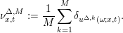
Note that, as in any Monte Carlo method, the approximation  ${\it\nu}^{{\rm\Delta},M}$ depends on the choice of
 ${\it\omega}\in {\rm\Omega}$, that is, the choice of seed in the random number generator. However, one can prove that the quality of approximation is independent of this choice,
 $\mathsf{P}$-almost surely.
Theorem 4.5. Algorithm 4.4 converges  $\mathsf{P}$-almost surely for some subsequence
 $M_{n}\rightarrow \infty$:
 $$\begin{eqnarray}{\it\nu}^{{\rm\Delta}x,M_{n}}\overset{\ast }{\rightharpoonup }{\it\nu}^{{\rm\Delta}x}\quad \text{as }n\rightarrow \infty .\end{eqnarray}$$
Equivalently, for every  ${\it\psi}\in C_{0}(\mathbb{R}^{d}\times \mathbb{R}_{+})$ and
 $g\in C_{0}(\mathbb{R}^{N})$,
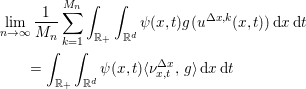 $$\begin{eqnarray}\displaystyle & & \displaystyle \lim _{n\rightarrow \infty }\frac{1}{M_{n}}\mathop{\sum }_{k=1}^{M_{n}}\int _{\mathbb{R}_{+}}\int _{\mathbb{R}^{d}}{\it\psi}(x,t)g(u^{{\rm\Delta}x,k}(x,t))\,\text{d}x\,\text{d}t\nonumber\\ \displaystyle & & \displaystyle \qquad =\int _{\mathbb{R}_{+}}\int _{\mathbb{R}^{d}}{\it\psi}(x,t)\langle {\it\nu}_{x,t}^{{\rm\Delta}x},\,g\rangle \,\text{d}x\,\text{d}t\end{eqnarray}$$
for  $\mathsf{P}$-almost every choice of
 ${\it\omega}\in {\rm\Omega}$. The above limits are uniform in
 ${\rm\Delta}x$.
The proof, provided in Fjordholm et al. (Reference Fjordholm, Käppeli, Mishra and Tadmor2016a, Appendix B), involves an adaptation of the law of large numbers in the present set-up of realizing the laws of measure-valued solutions using the Monte Carlo sampling procedure.
4.4 Interpretation of weak* convergence
The convergence of the approximate Young measures  ${\it\nu}^{{\rm\Delta}}$ generated by Algorithms 4.1 and 4.3 is in the weak* topology, that is,
 $$\begin{eqnarray}\displaystyle & & \displaystyle \int _{\mathbb{R}_{+}}\int _{\mathbb{R}}{\it\varphi}(x,t)\langle {\it\nu}_{x,t}^{{\rm\Delta}},g\rangle \,\text{d}x\,\text{d}t\rightarrow \int _{\mathbb{R}_{+}}\int _{\mathbb{R}}{\it\varphi}(x,t)\int _{\mathbb{R}^{N}}g(u)\,\text{d}{\it\nu}_{x,t}(u)\,\text{d}x\,\text{d}t\nonumber\\ \displaystyle & & \displaystyle \qquad +\int _{\mathbb{R}_{+}}\int _{\mathbb{R}}{\it\varphi}(x,t)\int _{S^{N-1}}g^{\infty }(z)\,\text{d}{\it\nu}_{x,t}^{\infty }(z)\,\text{d}{\it\lambda}(x,t)\end{eqnarray}$$
for all  ${\it\varphi}\in C_{0}(\mathbb{R}\times \mathbb{R}_{+})$ and for all
 $g\in C_{p}$. As described in Fjordholm et al. (Reference Fjordholm, Käppeli, Mishra and Tadmor2016a), this convergence amounts to convergence of statistics of functionals of interest. In particular, if
 $p\geq 1$ in (3.19), then we can choose
 $g({\it\xi})={\it\xi}$ to obtain the mean of the measure-valued solution; if
 $p\geq 2$ then the variance can be computed by choosing the test function
 $g({\it\xi})={\it\xi}\otimes {\it\xi}$. In practice, the goal of any numerical simulation is to accurately compute statistics of space-time averages of solution variables and to compare them to experimental or observational data. Thus, the weak* convergence of approximate Young measures, computed by Algorithms 4.1 and 4.3, provides an approximation of exactly these observable quantities of interest.
In order to compute statistics of space-time averages in (4.3), we need to compute phase space integrals with respect to the measure  ${\it\nu}^{{\rm\Delta}x}$:
 $$\begin{eqnarray}\langle {\it\nu}_{x,t}^{{\rm\Delta}x},\,g\rangle =\int _{\mathbb{ R}^{N}}g({\it\xi})\,\text{d}{\it\nu}_{x,t}^{{\rm\Delta}x}({\it\xi}),\quad g\in C(\mathbb{R}^{N}).\end{eqnarray}$$
The Monte Carlo method described in Algorithm 4.4 takes advantage of the representation of the measure  ${\it\nu}^{{\rm\Delta}x}$ as the law of a random field
 $u^{{\rm\Delta}x}$,
 $$\begin{eqnarray}\langle {\it\nu}_{x,t}^{{\rm\Delta}x},\,g\rangle :=\int _{\mathbb{ R}^{N}}g({\it\xi})\,\text{d}{\it\nu}_{x,t}^{{\rm\Delta}x}({\it\xi})=\int _{{\rm\Omega}}g(u^{{\rm\Delta}x}({\it\omega};x,t))\,\text{d}\mathsf{P}({\it\omega}),\end{eqnarray}$$
and replaces the integral over  ${\rm\Omega}$ with the approximation
 $$\begin{eqnarray}\langle {\it\nu}_{x,t}^{{\rm\Delta}x},\,g\rangle \approx \langle {\it\nu}^{{\rm\Delta}x,M},\,g\rangle =\frac{1}{M}\mathop{\sum }_{k=1}^{M}g(u^{{\rm\Delta}x,k}({\it\omega})).\end{eqnarray}$$
Thus, the space-time average (4.3) is approximated by
 $$\begin{eqnarray}\int _{\mathbb{R}_{+}}\int _{\mathbb{R}^{d}}{\it\varphi}(x,t)\langle {\it\nu}_{x,t}^{{\rm\Delta}x},\,g\rangle \,\text{d}x\,\text{d}t\approx \frac{1}{M}\mathop{\sum }_{k=1}^{M}\int _{\mathbb{R}_{+}}\int _{\mathbb{R}^{d}}{\it\varphi}(x,t)g(u^{{\rm\Delta}x,k}({\it\omega};x,t))\,\text{d}x\,\text{d}t.\end{eqnarray}$$
We note that the Monte Carlo sequence  $u^{{\rm\Delta}x,k}$ does not depend on the choice of the observable
 $g$; by Theorem 4.5, the same sequence
 $u^{{\rm\Delta}x,k}$ can be used for every observable. Hence, the Monte Carlo approximation
 ${\it\nu}^{{\rm\Delta}x,M}$ provides a unified approximation of all possible observables.
5 Systems of conservation laws
In this section we will provide details of numerical methods used in Step 2 of Algorithms 4.1 and 4.3 and describe convergence of these algorithms to dissipative measure-valued solutions of systems of conservation laws (2.1). We start with a description of numerical schemes for approximating conservation laws.
5.1 Numerical schemes for one- and multi-dimensional conservation laws
For simplicity, we begin with the description of a numerical scheme for the one-dimensional system of conservation laws (2.5). We discretize our computational domain into cells  ${\mathcal{C}}_{i}:=[x_{i-1/2},x_{i+1/2})$ with mesh size
 ${\rm\Delta}x=x_{i+1/2}-x_{i-1/2}$ and with midpoints
 $$\begin{eqnarray}x_{i}=\frac{x_{i-1/2}+x_{i+1/2}}{2}.\end{eqnarray}$$
Note that we consider a uniform mesh size  ${\rm\Delta}x$ only for the sake of simplicity of the exposition. Next, we discretize the one-dimensional system (2.5) with the following semi-discrete finite difference scheme for
 $u_{i}^{{\rm\Delta}x}(t)\equiv u^{{\rm\Delta}x}(x_{i},t)$:
 $$\begin{eqnarray}\begin{array}{@{}rl@{}}\frac{\text{d}}{\text{d}t}u_{i}^{{\rm\Delta}x}(t)+\frac{1}{{\rm\Delta}x}(F_{i+1/2}^{{\rm\Delta}x}(t)-F_{i-1/2}^{{\rm\Delta}x}(t))=0 & \quad t>0,~i\in \mathbb{Z},\\ u_{i}^{{\rm\Delta}x}(0)=u_{0}^{{\rm\Delta}x}(x_{i}) & \quad i\in \mathbb{Z}.\end{array}\end{eqnarray}$$
See, for example, Godlewski and Raviart (Reference Godlewski and Raviart1991), LeVeque (Reference LeVeque2002) and Tadmor (Reference Tadmor2012, Section 3.3). Here,  $u_{0}^{{\rm\Delta}x}$ is an approximation to the initial data
 $u_{0}$ using cell averages (for finite volume schemes) or cell midpoint values (for finite difference schemes). Henceforth, the dependence of
 $u$ and
 $F$ on
 ${\rm\Delta}x$ will be suppressed for notational convenience. Different schemes are specified by choosing different numerical flux functions,
 $F_{i+1/2}(t)$, which quantify the flux across the interface at
 $x_{i+1/2}$ as a function of the
 $2m$ neighbouring gridvalues
 $\{u(x_{j},t),j=i-m+1,\ldots ,i+m\}$, and are assumed to be consistent with the differential flux
 $f$ in the sense that
 $F(u,\ldots ,u)=f(u)$ for all
 $u\in \mathbb{R}^{N}$. For simplicity of exposition, we deal only with three-point schemes, that is,
 $m=1$.
The semi-discrete scheme (5.1a) needs to be integrated in time to define a fully discrete numerical approximation. Again for simplicity, we will use an exact time integration, resulting in
 $$\begin{eqnarray}u_{i}^{{\rm\Delta}x}(t+{\rm\Delta}t)=u_{i}^{{\rm\Delta}x}(t)-\frac{1}{{\rm\Delta}x}\int _{t}^{t+{\rm\Delta}t}(F_{i+1/2}({\it\tau})-F_{i-1/2}({\it\tau}))\,\text{d}{\it\tau}.\end{eqnarray}$$
We require that for all  ${\rm\Delta}x>0$ and
 $i\in \mathbb{N}$, the function
 $t\mapsto u(x_{i},t)$ is differentiable almost everywhere. We denote the evolution operator associated with the one-dimensional scheme (5.1) with mesh size
 ${\rm\Delta}x$ by
 $\mathbf{S}_{t}^{{\rm\Delta}x}$, so that
 $u^{{\rm\Delta}x}(\cdot ,t)=\mathbf{S}_{t}^{{\rm\Delta}x}u_{0}^{{\rm\Delta}x}$.
A similar framework applies to systems of conservation laws in several space dimensions. To simplify the notation we restrict ourselves to the two-dimensional case: we relabel the spatial variables  $(x_{1},x_{2})\mapsto (x,y)$ so that these equations take the form
 $$\begin{eqnarray}\partial _{t}u+\partial _{x}f^{x}(u)+\partial _{y}f^{y}(u)=0.\end{eqnarray}$$
We discretize our two-dimensional computational domain into cells with mesh size  ${\rm\Delta}:=({\rm\Delta}x,{\rm\Delta}y)$. The resulting two-dimensional cells
 $$\begin{eqnarray}{\mathcal{C}}_{i,j}:=[x_{i-1/2},x_{i+1/2})\times [y_{j-1/2},y_{j+1/2})\end{eqnarray}$$
are assumed to have a fixed mesh ratio,  ${\rm\Delta}x=x_{i+1/2}-x_{i-1/2}$ and
 ${\rm\Delta}y=y_{j+1/2}-y_{j-1/2}$, such that
 ${\rm\Delta}y=c{\rm\Delta}x$ for some constant
 $c>0$. Further, let
 $$\begin{eqnarray}x_{i}=\frac{x_{i-1/2}+x_{i+1/2}}{2},\quad y_{j}=\frac{y_{j-1/2}+y_{j+1/2}}{2}.\end{eqnarray}$$
We end up with the following semi-discrete finite difference scheme for  $u_{ij}^{{\rm\Delta}x,{\rm\Delta}y}=u^{{\rm\Delta}x,{\rm\Delta}y}(x_{i},y_{j},t)$:
 $$\begin{eqnarray}\displaystyle \begin{array}{@{}c@{}}\frac{\text{d}}{\text{d}t}u_{ij}^{{\rm\Delta}x,{\rm\Delta}y}(t)+\frac{1}{{\rm\Delta}x}(F_{i+1/2,j}^{x,{\rm\Delta}x}(t)-F_{i-1/2.j}^{x,{\rm\Delta}x}(t))\\ \quad \quad \quad \quad \quad \quad \quad +\frac{1}{{\rm\Delta}y}(F_{i,j+1/2}^{y,{\rm\Delta}y}(t)-F_{i,j-1/2}^{y,{\rm\Delta}y}(t))=0,\\ \;\quad \quad \quad \qquad u_{ij}^{{\rm\Delta}x,{\rm\Delta}y}(0)=u_{0}^{{\rm\Delta}x,{\rm\Delta}y}(x_{i},y_{j})\end{array} & & \displaystyle\end{eqnarray}$$
for all  $i,j\in \mathbb{Z}$ and
 $t>0$ (see again LeVeque Reference LeVeque2002, Godlewski and Raviart Reference Godlewski and Raviart1991). Here,
 $u_{0}^{{\rm\Delta}x,{\rm\Delta}y}\approx u_{0}$ is the approximate initial data and
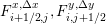 $F_{i+1/2,j}^{x,{\rm\Delta}x},F_{i,j+1/2}^{y,{\rm\Delta}y}$ are the numerical flux functions which are assumed to be consistent with the flux function
 $f=(f^{x},f^{y})$. We integrate the semi-discrete scheme (5.3a) exactly in time to obtain
 $$\begin{eqnarray}\displaystyle u_{ij}^{{\rm\Delta}x,{\rm\Delta}y}(t+{\rm\Delta}t) & = & \displaystyle u_{ij}^{{\rm\Delta}x,{\rm\Delta}y}(t)-\frac{1}{{\rm\Delta}x}\int _{t}^{t+{\rm\Delta}t}(F_{i+1/2,j}^{x,{\rm\Delta}x}({\it\tau})-F_{i-1/2,j}^{x,{\rm\Delta}x}({\it\tau}))\,\text{d}{\it\tau}\nonumber\\ \displaystyle & & \displaystyle \qquad -\frac{1}{{\rm\Delta}y}\int _{t}^{t+{\rm\Delta}t}(F_{i,j+1/2}^{y,{\rm\Delta}y}({\it\tau})-F_{i,j-1/2}^{y,{\rm\Delta}y}({\it\tau}))\,\text{d}{\it\tau}.\end{eqnarray}$$
We let  $\mathbf{S}_{t}^{{\rm\Delta}}$ denote the evolution operator corresponding to (5.3).
5.2 Weak* convergence to measure-valued solutions
We use the numerical evolution operator  $\mathbf{S}_{t}^{{\rm\Delta}x}$ in Step 2 of Algorithm 4.1 so that realizations of the initial random field
 $u_{0}({\it\omega})$ are evolved using finite volume (difference) schemes such as (5.1a). We show that the resulting approximate Young measures
 ${\it\nu}^{{\rm\Delta}x}$ converge weak* (up to a subsequence) to a dissipative measure-valued solution of systems of conservation laws as
 ${\rm\Delta}x\rightarrow 0$. We begin with the one-dimensional case (2.5).
Theorem 5.1. Let the one-dimensional system of conservation laws (2.5) be equipped with a strictly convex entropy  ${\it\eta}$ that satisfies the growth condition (3.19) with
 $p\geq 1$. Moreover, assume that
 $$\begin{eqnarray}|f(u)|\leq C(1+|u|^{r}),\quad |f^{\prime }(u)|\leq C(1+|u|^{r-1})\quad \text{for all}~u\in \mathbb{R}^{N}\end{eqnarray}$$
for some  $r\leq p$. Assume that the approximate solutions
 $u^{{\rm\Delta}x}$ generated by the numerical scheme (5.1a) satisfy the following conditions.
∙ Weak bounded variation. There exists an exponent
$s\geq p/(p-r+1)$ such that the following (fractional) bounded variation (BV) estimate of order $s$ holds: (5.5)for all$$\begin{eqnarray}\displaystyle \lim _{{\rm\Delta}x\rightarrow 0}\int _{0}^{T}\mathop{\sum }_{i}|u_{i+1}^{{\rm\Delta}x}({\it\omega};t)-u_{i}^{{\rm\Delta}x}({\it\omega};t)|^{s}{\rm\Delta}x\,\text{d}t=0 & & \displaystyle\end{eqnarray}$$${\it\omega}\in {\rm\Omega}$.∙ Entropy consistency. The numerical scheme (5.1a) is entropy-stable with respect to
$({\it\eta},q)$ in the sense that there exists a numerical entropy flux consistent with the entropy flux$$\begin{eqnarray}Q_{i+1/2}^{{\rm\Delta}x}(t)=Q(u_{i}^{{\rm\Delta}x}(t),u_{i+1}^{{\rm\Delta}x}(t)),\end{eqnarray}$$$q$, such that computed solutions satisfy the discrete entropy inequality (5.6)for all$$\begin{eqnarray}\displaystyle \frac{\text{d}}{\text{d}t}{\it\eta}(u_{i}^{{\rm\Delta}x})+\frac{1}{{\rm\Delta}x}(Q_{i+1/2}^{{\rm\Delta}x}-Q_{i-1/2}^{{\rm\Delta}x})\leq 0 & & \displaystyle\end{eqnarray}$$$t>0$, $i\in \mathbb{Z}$, ${\it\omega}\in {\rm\Omega}$.∙ Local Lipschitz continuity. The numerical flux function is locally Lipschitz in the sense that
(5.7)for all$$\begin{eqnarray}|F_{i+1/2}-f(u_{i})|\leq C(1+\max (|u_{i}|^{r-1},|u_{i+1}|^{r-1}))|u_{i+1}-u_{i}|\end{eqnarray}$$$u_{i},u_{i+1}\in \mathbb{R}^{N}$.∙ Consistency with initial data. If
${\it\sigma}^{{\rm\Delta}x}$ is the law of $u_{0}^{{\rm\Delta}x}$, then (5.8)for all$$\begin{eqnarray}\lim _{{\rm\Delta}x\rightarrow 0}\int _{\mathbb{R}}{\it\psi}(x)\langle {\it\sigma}_{x}^{{\rm\Delta}x},\,{\it\xi}\rangle \,\text{d}x=\int _{\mathbb{ R}}{\it\psi}(x)\langle {\it\sigma}_{x},\,{\it\xi}\rangle \,\text{d}x\end{eqnarray}$$${\it\psi}\in C_{c}^{1}(\mathbb{R})$, and (5.9)for all$$\begin{eqnarray}\limsup _{{\rm\Delta}x\rightarrow 0}\int _{\mathbb{R}}{\it\psi}(x)\langle {\it\sigma}_{x}^{{\rm\Delta}x},\,{\it\eta}\rangle \,\text{d}x\leq \int _{\mathbb{ R}}{\it\psi}(x)\langle {\it\sigma}_{x},\,{\it\eta}\rangle \,\text{d}x\end{eqnarray}$$$0\leq {\it\psi}\in C_{c}^{1}(\mathbb{R})$.












Then the approximate Young measures  ${\it\nu}^{{\rm\Delta}x}$ generated by Algorithm 4.1 converge weak* (up to a subsequence) as
 ${\rm\Delta}x\rightarrow 0$ to a dissipative measure-valued solution
 $({\it\nu},{\it\lambda},{\it\nu}^{\infty })$ of (2.5) with initial data
 ${\it\sigma}$.
Remark 5.2. If the approximate solution is uniformly bounded, that is,
 $$\begin{eqnarray}\Vert u^{{\rm\Delta}x}({\it\omega};\cdot ,t)\Vert \leq C<\infty\end{eqnarray}$$
for all  $t$ and for almost all
 ${\it\omega}\in {\rm\Omega}$, then the convergence stated in Theorem 5.1 follows under the weak BV estimate (5.5) (Fjordholm et al. Reference Fjordholm, Käppeli, Mishra and Tadmor2016a, Theorems 6,7). Here, convergence is established under the weaker assumption of an
 $L^{p}$ bound which is adapted to an entropy bound with an
 $L^{p}$ growth,
 ${\it\eta}(u)\sim |u|^{p}$.
Proof. By integrating the discrete entropy inequality (5.6) in time, we see that for all  $t$
 $$\begin{eqnarray}\int _{\mathbb{R}}{\it\eta}(u^{{\rm\Delta}x}({\it\omega};x,t))\,\text{d}x\leq C\quad \text{for all}~{\it\omega}\in {\rm\Omega}.\end{eqnarray}$$
Hence, the strict convexity condition (3.19) implies the uniform  $L^{p}$ bound
 $$\begin{eqnarray}\Vert u^{{\rm\Delta}x}\Vert _{p}:=\biggl(\int _{{\rm\Omega}}\int _{0}^{T}\mathop{\sum }_{i}|u_{i}^{{\rm\Delta}x}|^{p}~{\rm\Delta}x\,\text{d}t\,\text{d}\mathsf{P}\biggr)^{1/p}<C.\end{eqnarray}$$
Hence,
 $$\begin{eqnarray}\int _{0}^{T}\int _{\mathbb{R}}\langle {\it\nu}_{x,t}^{{\rm\Delta}x},\,|{\it\xi}|^{p}\rangle \,\text{d}x\,\text{d}t<C,\end{eqnarray}$$
so by the fundamental theorem of generalized Young measures, there exist a generalized Young measure  $({\it\nu},{\it\lambda},{\it\nu}^{\infty })$ on
 $\mathbb{R}\times [0,T]$ and a subsequence of
 ${\it\nu}^{{\rm\Delta}x}$ (still indexed by
 ${\rm\Delta}x$) such that
 ${\it\nu}^{{\rm\Delta}x}\overset{\ast }{\rightharpoonup }({\it\nu},{\it\lambda},{\it\nu}^{\infty })$ as
 ${\rm\Delta}x\rightarrow 0$. We show below that this generalized Young measure is indeed a dissipative measure-valued solution of the conservation law.
To this end, we multiply the finite volume scheme (5.1a) by  ${\it\varphi}(x_{i},t)$ for some
 ${\it\varphi}\in C_{c}^{\infty }(\mathbb{R}\times \mathbb{R}_{+})$ and by integrating and summing over
 $x\in \mathbb{R}$,
 ${\it\omega}\in {\rm\Omega}$,
 $i\in \mathbb{Z}$ yields
 $$\begin{eqnarray}\displaystyle 0 & = & \displaystyle \int _{{\rm\Omega}}\int _{0}^{T}\mathop{\sum }_{i}\frac{\text{d}u_{i}^{{\rm\Delta}x}}{\text{d}t}({\it\omega};t){\it\varphi}(x_{i},t)\nonumber\\ \displaystyle & & \displaystyle \qquad +\frac{F_{i+1/2}({\it\omega};t)-F_{i-1/2}({\it\omega};t)}{{\rm\Delta}x}{\it\varphi}(x_{i},t)~{\rm\Delta}x\,\text{d}t\,\text{d}\mathsf{P}\nonumber\\ \displaystyle & = & \displaystyle -\int _{{\rm\Omega}}\mathop{\sum }_{i}u_{i}^{{\rm\Delta}x}({\it\omega};0){\it\varphi}(x_{i},0)~{\rm\Delta}x\,\text{d}\mathsf{P}\nonumber\\ \displaystyle & & \displaystyle \qquad -\int _{{\rm\Omega}}\int _{0}^{T}\mathop{\sum }_{i}u_{i}^{{\rm\Delta}x}({\it\omega};t)\frac{\partial {\it\varphi}}{\partial t}(x_{i},t)~{\rm\Delta}x\,\text{d}t\,\text{d}\mathsf{P}\nonumber\\ \displaystyle & & \displaystyle \qquad -\underbrace{\int _{{\rm\Omega}}\int _{0}^{T}\mathop{\sum }_{i}F_{i+1/2}({\it\omega};t)\frac{{\it\varphi}(x_{i+1},t)-{\it\varphi}(x_{i},t)}{{\rm\Delta}x}~{\rm\Delta}x\,\text{d}t\,\text{d}\mathsf{P}}_{=\,{\mathcal{A}}}.\nonumber\end{eqnarray}$$
Using the equivalence of random fields and Young measures and the consistency with initial data (5.8), we observe that the first term converges to
 $$\begin{eqnarray}-\int _{\mathbb{R}}\langle {\it\sigma}_{x},{\it\xi}\rangle {\it\varphi}(x,0)\,\text{d}x,\end{eqnarray}$$
while the second term converges to
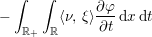 $$\begin{eqnarray}-\int _{\mathbb{R}_{+}}\int _{\mathbb{R}}\langle {\it\nu},\,{\it\xi}\rangle \frac{\partial {\it\varphi}}{\partial t}\,\text{d}x\,\text{d}t\end{eqnarray}$$
as  ${\rm\Delta}x\rightarrow 0$. We claim that the third term
 ${\mathcal{A}}$ converges to
 $$\begin{eqnarray}\int _{\mathbb{R}_{+}}\int _{\mathbb{R}}\langle {\it\nu},\,f\rangle \frac{\partial {\it\varphi}}{\partial x}\,\text{d}x\,\text{d}t+\int _{\mathbb{R}_{+}}\int _{\mathbb{R}}\langle {\it\nu}^{\infty },\,f^{\infty }\rangle \frac{\partial {\it\varphi}}{\partial x}\,\text{d}{\it\lambda},\end{eqnarray}$$
thus proving that  $({\it\nu},{\it\lambda},{\it\nu}^{\infty })$ is a measure-valued solution of (2.5). We have
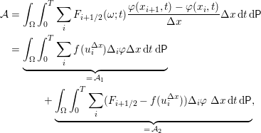 $$\begin{eqnarray}\displaystyle {\mathcal{A}} & = & \displaystyle \int _{{\rm\Omega}}\int _{0}^{T}\mathop{\sum }_{i}F_{i+1/2}({\it\omega};t)\frac{{\it\varphi}(x_{i+1},t)-{\it\varphi}(x_{i},t)}{{\rm\Delta}x}{\rm\Delta}x\,\text{d}t\,\text{d}\mathsf{P}\nonumber\\ \displaystyle & = & \displaystyle \underbrace{\int _{{\rm\Omega}}\int _{0}^{T}\mathop{\sum }_{i}f(u_{i}^{{\rm\Delta}x}){\rm\Delta}_{i}{\it\varphi}{\rm\Delta}x\,\text{d}t\,\text{d}\mathsf{P}}_{=\,{\mathcal{A}}_{1}}\nonumber\\ \displaystyle & & \displaystyle \qquad +\underbrace{\int _{{\rm\Omega}}\int _{0}^{T}\mathop{\sum }_{i}(F_{i+1/2}-f(u_{i}^{{\rm\Delta}x})){\rm\Delta}_{i}{\it\varphi}~{\rm\Delta}x\,\text{d}t\,\text{d}\mathsf{P}}_{=\,{\mathcal{A}}_{2}},\end{eqnarray}$$
where we let
 $$\begin{eqnarray}{\rm\Delta}_{i}{\it\varphi}=\frac{{\it\varphi}(x_{i+1},t)-{\it\varphi}(x_{i},t)}{{\rm\Delta}x}.\end{eqnarray}$$
For the first term in (5.11) we have
 $$\begin{eqnarray}\displaystyle {\mathcal{A}}_{1} & = & \displaystyle \int _{{\rm\Omega}}\int _{0}^{T}\mathop{\sum }_{i}f(u_{i}^{{\rm\Delta}x}){\rm\Delta}_{i}{\it\varphi}{\rm\Delta}x\,\text{d}t\,\text{d}\mathsf{P}\nonumber\\ \displaystyle & = & \displaystyle \underbrace{\int _{{\rm\Omega}}\int _{\mathbb{R}_{+}}\int _{\mathbb{R}}f(u^{{\rm\Delta}x}){\it\varphi}_{x}\,\text{d}x\,\text{d}t\,\text{d}\mathsf{P}}_{=\,{\mathcal{A}}_{1,1}}\nonumber\\ \displaystyle & & \displaystyle \qquad +\underbrace{\int _{\mathsf{P}}\int _{0}^{T}\mathop{\sum }_{i}f(u_{i}^{{\rm\Delta}x})({\rm\Delta}_{i}{\it\varphi}-{\rm\Delta}_{i-1/2}{\it\varphi})~{\rm\Delta}x\,\text{d}t\,\text{d}\mathsf{P}}_{=\,{\mathcal{A}}_{1,2}},\nonumber\end{eqnarray}$$
where
 $$\begin{eqnarray}{\rm\Delta}_{i-1/2}{\it\varphi}=\frac{{\it\varphi}(x_{i+1/2},t)-{\it\varphi}(x_{i-1/2},t)}{{\rm\Delta}x}=\frac{1}{{\rm\Delta}x}\int _{{\mathcal{C}}_{i}^{{\rm\Delta}x}}\partial _{x}{\it\varphi}\,\text{d}x.\end{eqnarray}$$
By the fundamental theorem of Young measures, the first term  ${\mathcal{A}}_{1,1}$ converges to
 $$\begin{eqnarray}\int _{\mathbb{R}_{+}}\int _{\mathbb{R}}\langle {\it\nu},\,f\rangle \frac{\partial {\it\varphi}}{\partial x}\,\text{d}x\,\text{d}t+\int _{\mathbb{R}_{+}}\int _{\mathbb{R}}\langle {\it\nu}^{\infty },\,f^{\infty }\rangle \frac{\partial {\it\varphi}}{\partial x}\,\text{d}{\it\lambda}_{t}(x)\,\text{d}t.\end{eqnarray}$$
The term  ${\mathcal{A}}_{1,2}$ vanishes as
 ${\rm\Delta}x\rightarrow 0$:
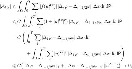 $$\begin{eqnarray}\displaystyle |{\mathcal{A}}_{1,2}| & \leq & \displaystyle \int _{{\rm\Omega}}\int _{0}^{T}\mathop{\sum }_{i}|f(u_{i}^{{\rm\Delta}x})|\,|{\rm\Delta}_{i}{\it\varphi}-{\rm\Delta}_{i-1/2}{\it\varphi}|~{\rm\Delta}x\,\text{d}t\,\text{d}\mathsf{P}\nonumber\\ \displaystyle & \leq & \displaystyle C\int _{{\rm\Omega}}\int _{0}^{T}\mathop{\sum }_{i}(1+|u_{i}^{{\rm\Delta}x}|^{r})\,|{\rm\Delta}_{i}{\it\varphi}-{\rm\Delta}_{i-1/2}{\it\varphi}|~{\rm\Delta}x\,\text{d}t\,\text{d}\mathsf{P}\nonumber\\ \displaystyle & = & \displaystyle C\left(\int _{0}^{T}\mathop{\sum }_{i}|{\rm\Delta}_{i}{\it\varphi}-{\rm\Delta}_{i-1/2}{\it\varphi}|~{\rm\Delta}x\,\text{d}t\right.\nonumber\\ \displaystyle & & \displaystyle \qquad +\left.\int _{{\rm\Omega}}\int _{0}^{T}\mathop{\sum }_{i}|u_{i}^{{\rm\Delta}x}|^{r}\,|{\rm\Delta}_{i}{\it\varphi}-{\rm\Delta}_{i-1/2}{\it\varphi}|~{\rm\Delta}x\,\text{d}t\,\text{d}\mathsf{P}\right)\nonumber\\ \displaystyle & \leq & \displaystyle C(\Vert {\rm\Delta}{\it\varphi}-{\rm\Delta}_{\cdot -1/2}{\it\varphi}\Vert _{1}+\Vert {\rm\Delta}{\it\varphi}-{\rm\Delta}_{\cdot -1/2}{\it\varphi}\Vert _{a^{\prime }}\,\Vert u^{{\rm\Delta}x}\Vert _{p}^{r})\rightarrow 0,\nonumber\end{eqnarray}$$
where we have used Hölder’s inequality with exponent  $a=p/r\geq 1$, the fact that
 ${\rm\Delta}{\it\varphi}-{\rm\Delta}_{\cdot -1/2}{\it\varphi}\rightarrow 0$ in both
 $L^{1}$ and
 $L^{a^{\prime }}$, and (5.10).
To bound the second term in (5.11), we apply (5.7) to obtain
 $$\begin{eqnarray}\displaystyle |{\mathcal{A}}_{2}| & \leq & \displaystyle C\underbrace{\int _{{\rm\Omega}}\int _{0}^{T}\mathop{\sum }_{i}|u_{i+1}^{{\rm\Delta}x}-u_{i}^{{\rm\Delta}x}|\,|{\rm\Delta}_{i}{\it\varphi}|~{\rm\Delta}x\,\text{d}t\,\text{d}\mathsf{P}}_{=\,{\mathcal{A}}_{2,1}}\nonumber\\ \displaystyle & & \displaystyle \qquad +C\underbrace{\int _{{\rm\Omega}}\int _{0}^{T}\mathop{\sum }_{i}|u_{i}^{{\rm\Delta}x}|^{r-1}\,|u_{i+1}^{{\rm\Delta}x}-u_{i}^{{\rm\Delta}x}|\,|{\rm\Delta}_{i}{\it\varphi}|~{\rm\Delta}x\,\text{d}t\,\text{d}\mathsf{P}}_{=\,{\mathcal{A}}_{2,2}}\nonumber\\ \displaystyle & & \displaystyle \qquad +C\underbrace{\int _{{\rm\Omega}}\int _{0}^{T}\mathop{\sum }_{i}|u_{i+1}^{{\rm\Delta}x}|^{r-1}\,|u_{i+1}^{{\rm\Delta}x}-u_{i}^{{\rm\Delta}x}|\,|{\rm\Delta}_{i}{\it\varphi}|~{\rm\Delta}x\,\text{d}t\,\text{d}\mathsf{P}}_{=\,{\mathcal{A}}_{2,3}}.\nonumber\end{eqnarray}$$
Denote
 $$\begin{eqnarray}\Vert \unicode[STIX]{x27E6}u^{{\rm\Delta}x}\unicode[STIX]{x27E7}\Vert _{s}:=\biggl(\int _{{\rm\Omega}}\int _{0}^{T}\mathop{\sum }_{i}|u_{i+1}^{{\rm\Delta}x}(t)-u_{i}^{{\rm\Delta}x}(t)|^{s}~{\rm\Delta}x\,\text{d}t\,\text{d}\mathsf{P}\biggr)^{1/s}\rightarrow 0\end{eqnarray}$$
as  ${\rm\Delta}x\rightarrow 0$, where the limit follows from (5.5). For the first term in
 ${\mathcal{A}}_{2,1}$ we have
 $$\begin{eqnarray}\displaystyle {\mathcal{A}}_{2,1}=\int _{{\rm\Omega}}\int _{0}^{T}\mathop{\sum }_{i}|u_{i+1}^{{\rm\Delta}x}-u_{i}^{{\rm\Delta}x}|\,|{\rm\Delta}_{i}{\it\varphi}|~{\rm\Delta}x\,\text{d}t\,\text{d}\mathsf{P}\leq \Vert \unicode[STIX]{x27E6}u^{{\rm\Delta}x}\unicode[STIX]{x27E7}\Vert _{s}\,\Vert {\it\varphi}_{x}\Vert _{s^{\prime }}\rightarrow 0 & & \displaystyle \nonumber\end{eqnarray}$$
as  ${\rm\Delta}x\rightarrow 0$, by Hölder’s inequality and (5.12). The terms
 ${\mathcal{A}}_{2,2}$ and
 ${\mathcal{A}}_{2,3}$ behave the same way as
 ${\rm\Delta}x\rightarrow 0$, so it suffices to show that the first one vanishes as
 ${\rm\Delta}x\rightarrow 0$. Indeed, for
 $s\geq p/(p-r+1)$, there exists
 $a\in [1,\infty ]$ such that the generalized Hölder’s inequality with exponents
 $(p/(r-1),s,a)$ implies
 $$\begin{eqnarray}\displaystyle & & \displaystyle \int _{{\rm\Omega}}\int _{0}^{T}\mathop{\sum }_{i}|u_{i}^{{\rm\Delta}x}|^{r-1}\,|u_{i+1}^{{\rm\Delta}x}-u_{i}^{{\rm\Delta}x}|\,|{\rm\Delta}_{i}{\it\varphi}|~{\rm\Delta}x\,\text{d}t\,\text{d}\mathsf{P}\nonumber\\ \displaystyle & & \displaystyle \qquad \leq \Vert u^{{\rm\Delta}x}\Vert _{p}^{r-1}\,\Vert \unicode[STIX]{x27E6}u^{{\rm\Delta}x}\unicode[STIX]{x27E7}\Vert _{s}\,\Vert {\rm\Delta}{\it\varphi}\Vert _{a},\quad \text{for}~~\frac{r-1}{p}+\frac{1}{s}+\frac{1}{a}=1.\nonumber\end{eqnarray}$$
We conclude that
 $$\begin{eqnarray}{\mathcal{A}}_{2,2}+{\mathcal{A}}_{2,3}\leq 2\Vert u^{{\rm\Delta}x}\Vert _{p}^{r-1}\,\Vert \unicode[STIX]{x27E6}u^{{\rm\Delta}x}\unicode[STIX]{x27E7}\Vert _{s}\,\Vert {\rm\Delta}{\it\varphi}\Vert _{a}\rightarrow 0\end{eqnarray}$$
as  ${\rm\Delta}x\rightarrow 0$, by (5.10) and (5.12).
The proof of convergence to a dissipative measure-valued solution (i.e., consistency with (3.22)) in the limit  ${\rm\Delta}x\rightarrow 0$ is a straightforward adaptation of the above proof to the discrete entropy inequality (5.6).◻
Theorem 5.1 can be readily extended to several space dimensions. We present the two-dimensional version.
Theorem 5.3. Let the two-dimensional system of conservation laws (5.2) be equipped with a strictly convex entropy  $S$ that satisfies the growth condition (3.19) with
 $p\geq 1$. Moreover, assume that
 $$\begin{eqnarray}|f(u)|\leq C(1+|u|^{r}),\quad |{\rm\nabla}f(u)|\leq C(1+|u|^{r-1})\quad \text{for all}~u\in \mathbb{R}^{N}\end{eqnarray}$$
for some  $r\leq p$. Assume that the approximate solutions
 $u^{{\rm\Delta}}$ generated by the numerical scheme (5.3a) satisfy the following conditions.
∙ Weak bounded variation. There exists an exponent
$s\geq p/(p-r+1)$ such that the following (fractional) BV estimate of order $s$ holds: (5.14)for all$$\begin{eqnarray}\displaystyle & & \displaystyle \lim _{{\rm\Delta}\rightarrow 0}\int _{0}^{T}\mathop{\sum }_{i,j}\left(|u_{i+1,j}^{{\rm\Delta}}({\it\omega};t)-u_{i,j}^{{\rm\Delta}}({\it\omega};t)|^{s}\right.\nonumber\\ \displaystyle & & \displaystyle \qquad \left.+|u_{i,j+1}^{{\rm\Delta}}({\it\omega};t)-u_{i,j}^{{\rm\Delta}}({\it\omega};t)|^{s}\right)\,{\rm\Delta}x\,{\rm\Delta}y\,\text{d}t=0\end{eqnarray}$$${\it\omega}\in {\rm\Omega}$.∙ Entropy consistency. The numerical scheme (5.3a) is entropy-stable with respect to
$({\it\eta},q)$ in the sense that there exist numerical entropy fluxes $Q_{i+1/2,j}^{x}$, $Q_{i,j+1/2}^{y}$, consistent with the entropy flux $q$, such that computed solutions satisfy the discrete entropy inequality (5.15)for all$$\begin{eqnarray}\displaystyle \frac{\text{d}}{\text{d}t}{\it\eta}(u_{i,j}^{{\rm\Delta}})+\frac{1}{{\rm\Delta}x}(Q_{i+1/2,j}^{x}-Q_{i-1/2,j}^{x})+\frac{1}{{\rm\Delta}y}(Q_{i,j+1/2}^{y}-Q_{i,j-1/2}^{y})\leq 0, & & \displaystyle\end{eqnarray}$$$t>0$, $i,j\in \mathbb{Z}$, ${\it\omega}\in {\rm\Omega}$.∙ Local Lipschitz continuity. The numerical flux functions are locally Lipschitz, that is, they satisfy
(5.16)for all$$\begin{eqnarray}\displaystyle |F_{i+1/2,j}^{x}-f^{x}(u_{i,j}^{{\rm\Delta}})| & \leq & \displaystyle C(1+\max (|u_{i,j}^{{\rm\Delta}}|^{r-1},|u_{i+1,j}^{{\rm\Delta}}|^{r-1}))\,|u_{i+1,j}^{{\rm\Delta}}-u_{i,j}^{{\rm\Delta}}|,\nonumber\\ \displaystyle |F_{i,j+1/2}^{y}-f^{y}(u_{i,j}^{{\rm\Delta}})| & \leq & \displaystyle C(1+\max (|u_{i,j}^{{\rm\Delta}}|^{r-1},|u_{i,j+1}^{{\rm\Delta}}|^{r-1}))\,|u_{i,j+1}^{{\rm\Delta}}-u_{i,j}^{{\rm\Delta}}|,\nonumber\\ \displaystyle & & \displaystyle\end{eqnarray}$$$i,j\in \mathbb{Z}$.∙ Consistency with initial data. If
${\it\sigma}^{{\rm\Delta}x}$ is the law of $u_{0}^{{\rm\Delta}x}$, then it satisfies (5.8) and (5.9).


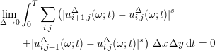








Then, the approximate Young measures  ${\it\nu}^{{\rm\Delta}}$ generated by Algorithm 4.1 converge weak* (up to a subsequence) as
 ${\rm\Delta}x,{\rm\Delta}y\rightarrow 0$ to a dissipative measure-valued solution
 $({\it\nu},{\it\lambda},{\it\nu}^{\infty })$ of (5.2) with initial data
 ${\it\sigma}$.
Combining the Monte Carlo convergence Theorem 4.5 with the convergence established in Theorems 5.1 and 5.3, we conclude with the following.
Corollary 5.4 (convergence with mesh refinement).
Under the assumptions of Theorem 5.1 (or Theorem 5.3 in two dimensions), there are subsequences  ${\rm\Delta}_{n}\rightarrow 0$ and
 $M_{n}\rightarrow \infty$ and a dissipative measure-valued solution
 $({\it\nu},{\it\lambda},{\it\nu}^{\infty })$ of (2.1) with initial data
 ${\it\sigma}$, such that
 $$\begin{eqnarray}{\it\nu}^{{\rm\Delta}_{n},M_{n}}\overset{\ast }{\rightharpoonup }({\it\nu},{\it\lambda},{\it\nu}^{\infty })\quad \text{as }n\rightarrow \infty .\end{eqnarray}$$
5.3 Convergence for atomic initial data
The special case of atomic initial data  ${\it\sigma}={\it\delta}_{u_{0}}$ requires us to use Algorithm 4.3 to compute underlying dissipative measure-valued solutions. We have the following convergence theorem for Algorithm 4.3 in the two-dimensional case.
Theorem 5.5. Consider the two-dimensional system of conservation laws (5.2). Let  $\{{\it\nu}^{{\rm\Delta},{\it\varepsilon}}\}_{{\rm\Delta},{\it\varepsilon}>0}$ be the family of approximate measure-valued solutions constructed by Algorithm 4.3 using the numerical scheme (5.3a). Then there exists a subsequence
 $({\rm\Delta}_{n},{\it\varepsilon}_{n})\rightarrow 0$ such that
 ${\it\nu}^{{\rm\Delta}_{n},{\it\varepsilon}_{n}}$ converges weak* to a dissipative measure-valued solution
 $({\it\nu},{\it\lambda},{\it\nu}^{\infty })$ with atomic initial data
 $u_{0}$.
Proof. By Theorem 5.3 we know that for every  ${\it\varepsilon}>0$ there exists a subsequence
 ${\rm\Delta}_{k}\rightarrow 0$ as
 $k\rightarrow \infty$ such that
 ${\it\nu}^{{\rm\Delta}_{k},{\it\varepsilon}}$ converges weak* as
 $k\rightarrow \infty$ to a dissipative measure-valued solution
 $({\it\nu}^{{\it\varepsilon}},{\it\lambda}^{{\it\varepsilon}},{\it\nu}^{\infty ,{\it\varepsilon}})$ of (5.2) with initial data
 ${\it\sigma}^{{\it\varepsilon}}$. Thus, (3.21) and (3.22) hold with
 $({\it\nu},{\it\lambda},{\it\nu}^{\infty })$ and
 ${\it\sigma}$ replaced by
 $({\it\nu}^{{\it\varepsilon}},{\it\lambda}^{{\it\varepsilon}},{\it\nu}^{\infty ,{\it\varepsilon}})$ and
 ${\it\sigma}^{{\it\varepsilon}}$, respectively. We abbreviate the corresponding statement of measure-valued solution and dissipative measure-valued solution by (3.21)
 $_{{\it\varepsilon}}$ and (3.22)
 $_{{\it\varepsilon}}$. The existence of a subsequence
 ${\it\varepsilon}_{m}\rightarrow 0$ as
 $m\rightarrow \infty$ such that
 $({\it\nu}^{{\it\varepsilon}_{m}},{\it\lambda}^{{\it\varepsilon}_{m}},{\it\nu}^{\infty ,{\it\varepsilon}_{m}})\overset{\ast }{\rightharpoonup }({\it\nu},{\it\lambda},{\it\nu}^{\infty })$ for some generalized Young measure
 $({\it\nu},{\it\lambda},{\it\nu}^{\infty })$, is a consequence of Theorem 3.3. The fact that
 $({\it\nu},{\it\lambda},{\it\nu}^{\infty })$ is a (dissipative) measure-valued solution follows at once by taking the limit
 ${\it\varepsilon}_{m}\rightarrow 0$ in (3.21)
 $_{{\it\varepsilon}_{m}}$ and (3.22)
 $_{{\it\varepsilon}_{m}}$. Finally, we extract a diagonal sequence
 $\{({\rm\Delta}_{n},{\it\varepsilon}_{n})\}_{n\in \mathbb{N}}$ such that
 ${\it\nu}^{{\rm\Delta}_{n},{\it\varepsilon}_{n}}\overset{\ast }{\rightharpoonup }({\it\nu},{\it\lambda},{\it\nu}^{\infty })$.◻
5.4 Convergent schemes for scalar conservation laws
Monotone finite difference (volume) schemes (see Godlewski and Raviart Reference Godlewski and Raviart1991 for a precise definition) for scalar equations are uniformly bounded in  $L^{\infty }$ (as they satisfy a discrete maximum principle), satisfy a discrete entropy inequality (using the Crandall–Majda numerical entropy fluxes: Crandall and Majda Reference Crandall and Majda1980) and are total variation decreasing (TVD), that is, the total variation of the approximate solutions is non-increasing over time. Consequently, the approximate solutions satisfy the weak BV estimate (5.5) (resp. (5.14) in the multi-dimensional case) with
 $r=1$. Thus, monotone schemes, approximating scalar conservation laws, satisfy all the abstract criteria of Theorems 5.1 and 5.3. Furthermore, the uniform
 $L^{\infty }$ bound on approximations implies that there is no concentration and the limit is completely described by the Young measure
 ${\it\nu}$. In Fjordholm et al. (Reference Fjordholm, Käppeli, Mishra and Tadmor2016a) we have shown the following convergence theorem for monotone schemes of scalar conservation laws,
Theorem 5.6. Let  ${\it\nu}^{{\rm\Delta}x}$ be generated by Algorithm 4.1, and let
 ${\it\nu}$ be the law of the entropy solution
 $u({\it\omega})$. If
 $\text{TV}(u_{0}({\it\omega}))\leq C$ for all
 ${\it\omega}\in {\rm\Omega}$, then
 ${\it\nu}^{{\rm\Delta}x}\overset{\ast }{\rightharpoonup }{\it\nu}$ as
 ${\rm\Delta}x\rightarrow 0$.
5.5 Convergent schemes for systems of conservation laws
We know of at least three classes of numerical methods that satisfy the criteria of convergence Theorems 5.1 and 5.3.
5.5.1 The ELW scheme
The entropy-stable Lax–Wendroff (ELW) schemes introduced in Fjordholm (Reference Fjordholm2013, Section 4.2), are finite difference schemes of the form (5.1a) with a numerical flux of the form
 $$\begin{eqnarray}F_{i+1/2}:=\widetilde{F}_{i+1/2}^{(k)}-d_{i+1/2}|\unicode[STIX]{x27E6}v\unicode[STIX]{x27E7}_{i+1/2}|^{k-1}\unicode[STIX]{x27E6}v\unicode[STIX]{x27E7}_{i+1/2},\quad d_{i+1/2}>0.\end{eqnarray}$$
Here, the jump  $\unicode[STIX]{x27E6}v\unicode[STIX]{x27E7}_{i+1/2}:=v_{i+1}-v_{i}$ is expressed in terms of the entropy variables,
 $v:={\it\eta}^{\prime }(u)$, and
 $\widetilde{F}_{i+1/2}^{(k)}$ is a
 $k$th-order accurate entropy conservative numerical flux which is characterized by the compatibility requirement with the corresponding entropy flux
 $q(u)$, introduced in Tadmor (Reference Tadmor1987):
 $$\begin{eqnarray}\displaystyle \langle v_{i+1}-v_{i},\widetilde{F}_{i+1/2}^{(k)}\rangle ={\it\zeta}_{q}(v_{i+1})-{\it\zeta}_{q}(v_{i}),\quad {\it\zeta}_{q}(v):=\langle v,f(\!u(v)\rangle -q(u(v)). & & \displaystyle \nonumber\\ \displaystyle & & \displaystyle\end{eqnarray}$$
The schemes based on such fluxes  $\widetilde{F}_{i+1/2}^{(k)}$, that is, (5.17) and (5.18) with
 $d_{i+1/2}\equiv 0$, are entropy conservative in the sense of satisfying the equalities (5.6) and (5.15). This results in the desired entropy inequalities (5.6) and (5.15) by adding a judicious amount of
 $k$th-order numerical viscosity
 $d_{i+1/2}|\unicode[STIX]{x27E6}v\unicode[STIX]{x27E7}_{i+1/2}|^{k-1}\unicode[STIX]{x27E6}v\unicode[STIX]{x27E7}_{i+1/2}$ parametrized with positive viscosity amplitudes
 $d_{i+1/2}>0$.
A general class of such second-order entropy conservative fluxes was constructed in Tadmor (Reference Tadmor2003), and a particularly ‘affordable’ version for the compressible Euler equations was given in Ismail and Roe (Reference Ismail and Roe2009) in terms of the rescaled variables  $z:=({\it\rho}/p)^{1/2}(1,v_{1},v_{2},p)^{\top }$:
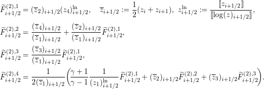 $$\begin{eqnarray}\displaystyle \widetilde{F}_{i+1/2}^{(2),1} & = & \displaystyle (\overline{z}_{2})_{i+1/2}(z_{4})_{i+1/2}^{\ln },\quad \overline{z}_{i+1/2}:=\frac{1}{2}(z_{i}+z_{i+1}),~z_{i+1/2}^{\ln }:=\frac{\unicode[STIX]{x27E6}z_{i+1/2}\unicode[STIX]{x27E7}}{\unicode[STIX]{x27E6}\log (z)_{i+1/2}\unicode[STIX]{x27E7}},\nonumber\\ \displaystyle \widetilde{F}_{i+1/2}^{(2),2} & = & \displaystyle \frac{(\overline{z}_{4})_{i+1/2}}{(\overline{z}_{1})_{i+1/2}}+\frac{(\overline{z}_{2})_{i+1/2}}{(\overline{z}_{1})_{i+1/2}}\widetilde{F}_{i+1/2}^{(2),1},\nonumber\\ \displaystyle \widetilde{F}_{i+1/2}^{(2),3} & = & \displaystyle \frac{(\overline{z}_{3})_{i+1/2}}{(\overline{z}_{1})_{i+1/2}}\widetilde{F}_{i+1/2}^{(2),1},\nonumber\\ \displaystyle \widetilde{F}_{i+1/2}^{(2),4} & = & \displaystyle \frac{1}{2(\overline{z}_{1})_{i+1/2}}\biggl(\!\frac{{\it\gamma}+1}{{\it\gamma}-1}\frac{1}{(z_{1})_{i+1/2}^{\ln }}\widetilde{F}_{i+1/2}^{(2),1}+(\overline{z}_{2})_{i+1/2}\widetilde{F}_{i+1/2}^{(2),2}+(\overline{z}_{3})_{i+1/2}\widetilde{F}_{i+1/2}^{(2),3}\!\biggr).\nonumber\end{eqnarray}$$
A general recipe to convert such second-order methods to arbitrarily high-order entropy conservative fluxes, 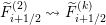 $\widetilde{F}_{i+1/2}^{(2)}{\rightsquigarrow}\widetilde{F}_{i+1/2}^{(k)}$, was derived in LeFloch, Mercier and Rohde (Reference LeFloch, Mercier and Rohde2002) and utilized in Fjordholm et al. (Reference Fjordholm, Mishra and Tadmor2012) and Fjordholm (Reference Fjordholm2013). The resulting ELW schemes are readily seen to be (i) (formally)
 $k$th-order accurate and (ii) entropy-stable in the sense of satisfying the entropy consistency (5.6) and (5.15), and (iii) they can be shown to satisfy the weak BV bounds (5.5) and (5.14) and converge strongly for scalar conservation laws (Fjordholm Reference Fjordholm2013, Propositions 4.2 and 4.3).
5.5.2 TeCNO finite difference schemes
The TeCNO schemes, introduced in Fjordholm et al. (Reference Fjordholm, Mishra and Tadmor2012) and Fjordholm (Reference Fjordholm2013), are finite difference schemes of the form (5.1a) with numerical flux
 $$\begin{eqnarray}F_{i+1/2}:=\widetilde{F}_{i+1/2}^{(k)}-\frac{1}{2}D_{i+1/2}(v_{i+1/2}^{+}-v_{i+1/2}^{-}).\end{eqnarray}$$
Here,  $\widetilde{F}_{i+1/2}^{(k)}$ is the same entropy conservative flux satisfying (5.18),
 $D_{i+1/2}$ is a positive definite (viscosity) matrix, and
 $v_{i+1/2}^{\pm }$ are the cell interface values obtained by the following
 $k$th-order accurate ENO reconstruction (Harten et al. Reference Harten, Engquist, Osher and Chakravarty1987). Specifically, starting with the given piecewise constant approximate solution,
 $\sum _{i}v_{i}1_{{\mathcal{C}}_{i}}(x)$, one constructs a piecewise polynomial approximation
 $v^{{\rm\Delta}}(x)$:
 $$\begin{eqnarray}\mathop{\sum }_{i}v_{i}1_{{\mathcal{C}}_{i}}(x)~~{\rightsquigarrow}~~v^{{\rm\Delta}}(x):=\mathop{\sum }_{i}p_{i}(x)1_{{\mathcal{C}}_{i}}(x),\end{eqnarray}$$
where  $\{p_{i}(x)\}$ are a judicious choice of
 $k$th-order accurate essentially non-oscillatory (ENO) polynomials introduced in Harten et al. (Reference Harten, Engquist, Osher and Chakravarty1987). We then set the ENO reconstructed pointvalues across the cell interface,
 $v_{i+1/2}^{\pm }=v^{{\rm\Delta}}(x_{i+1/2}\pm )$, namely,
 $$\begin{eqnarray}v_{i+1/2}^{+}=p_{i+1}(x_{i+1/2}),\quad v_{i+1/2}^{-}=p_{i}(x_{i+1/2}).\end{eqnarray}$$
The multi-dimensional (Cartesian) version was designed in Fjordholm et al. (Reference Fjordholm, Mishra and Tadmor2012) (see also Fjordholm Reference Fjordholm2013). The class of TeCNO schemes was shown by Fjordholm et al. (Reference Fjordholm, Mishra and Tadmor2012) and Fjordholm (Reference Fjordholm2013) to have the following properties.
∙ They are (formally)
$k$th-order accurate.∙ They are entropy-stable. Using the sign property
$\text{sign}(v_{i+1/2}^{+}-v_{i+1/2}^{-})=\text{sign}(v_{i+1}-v_{i})$ proved in Fjordholm, Mishra and Tadmor (Reference Fjordholm, Mishra and Tadmor2013), it follows that the TeCNO schemes are entropy-stable in the sense of satisfying the discrete entropy inequality (5.6), and the corresponding two-dimensional inequality (5.15) (Fjordholm et al. Reference Fjordholm, Mishra and Tadmor2012).∙ They have weakly bounded variation when
$k=1$ and $k=2$, that is, they satisfy a bound of the form (5.5) in the one-dimensional case and (5.14) in two dimensions; see Fjordholm (Reference Fjordholm2013, Theorem 6.6) and Fjordholm (Reference Fjordholm2013, Section 3.2) for the general multi-dimensional case. The weak total variation bound for $k\geq 3$ depends on a conjectured result for the ENO reconstruction method which remains to be proved; see Fjordholm (Reference Fjordholm2013, Section 5.5).




In light of these properties, the approximate measure-valued solutions generated by the TeCNO scheme converge to an EMV solution of (2.1).
5.5.3 Shock-capturing space-time discontinuous Galerkin schemes
Finite difference and finite volume schemes of the type (5.1a) are particularly suitable for Cartesian grids. For problems which involve spatial domains with complex geometries that necessitate the use of unstructured grids (triangles, tetrahedra), an alternative discretization procedure is the space-time discontinuous finite element procedure of Johnson and Szepessy (Reference Johnson and Szepessy1987), Jaffre, Johnson and Szepessy (Reference Jaffre, Johnson and Szepessy1995), Barth (Reference Barth, Kroner, Ohlberger and Rohde1999) and Hiltebrand and Mishra (Reference Hiltebrand and Mishra2014). In this discontinuous Galerkin (DG) procedure, entropy-stable numerical fluxes expressed in terms of the entropy variables, such as those in (5.19), are used at cell interfaces. Hiltebrand and Mishra (Reference Hiltebrand and Mishra2014) showed that the space-time DG method augmented with a shock-capturing streamline diffusion term satisfies a suitable version of the weak BV bound (5.5) and is entropy-stable in the sense of satisfying the discrete entropy inequality (5.15). Arguing along the lines of Hiltebrand and Mishra (Reference Hiltebrand and Mishra2014, Theorem 4.1), it follows that this DG method converges to a dissipative measure-valued solution of (2.1). We remark that the space-time DG methods are fully discrete, in contrast to semi-discrete finite difference schemes such as (5.1a).
6 Incompressible Euler equations
In this section we specify the numerical methods used in Step 2 of Algorithms 4.1 and 4.3 for computing admissible measure-valued solutions of the incompressible Euler equations (1.3). We review two sets of numerical methods: spectral methods and projection finite difference methods. We start with spectral methods.
6.1 Spectral (viscosity) methods for the incompressible Euler equations
6.1.1 The numerical method $\mathbf{S}_{t}^{N}$

Spectral methods approximate the Euler equations (1.3) in Fourier space (Gottlieb et al. Reference Gottlieb, Hussaini, Orszag and Voigt1984). Let  $\mathbb{T}^{d}$ denote the
 $d$-dimensional Torus. If
 $(u,p)$ is a solution of the Euler equation (1.3) with periodic boundary conditions, then (formally) it also satisfies the convective form of the equations
 $$\begin{eqnarray}\displaystyle \left\{\begin{array}{@{}r@{}}\partial _{t}u+u\cdot {\rm\nabla}u+{\rm\nabla}p=0\\ {\rm\nabla}_{x}\cdot u=0\end{array}\right.\quad \text{in }\mathbb{T}^{d}\times \mathbb{R}_{+}. & & \displaystyle\end{eqnarray}$$
Consider the spatial Fourier expansion
 $$\begin{eqnarray}u(x,t)=\mathop{\sum }_{k\in \mathbb{Z}^{d}}\widehat{u}_{k}(t)\,\text{e}^{\text{i}k\cdot x}\end{eqnarray}$$
with coefficients given by
 $$\begin{eqnarray}\displaystyle \widehat{u}_{k}(t)=\frac{1}{(2{\it\pi})^{d}}\int _{\mathbb{T}^{d}}u(x,t)\,\text{e}^{-\text{i}k\cdot x}\,\text{d}x,\quad k\in \mathbb{Z}^{d}. & & \displaystyle \nonumber\end{eqnarray}$$
If  $u$ is a solution of (6.1), the above expression yields
 $$\begin{eqnarray}\displaystyle \frac{\text{d}}{\text{d}t}\widehat{u}_{k} & = & \displaystyle \frac{1}{(2{\it\pi})^{d}}\int _{\mathbb{T}^{d}}u_{t}\,\text{e}^{-\text{i}k\cdot x}\,\text{d}x\nonumber\\ \displaystyle & = & \displaystyle -\frac{1}{(2{\it\pi})^{d}}\int _{\mathbb{T}^{d}}(u\cdot {\rm\nabla}u+{\rm\nabla}p)\,\text{e}^{-\text{i}k\cdot x}\,\text{d}x\nonumber\\ \displaystyle & = & \displaystyle -\frac{\text{i}}{(2{\it\pi})^{d}}\mathop{\sum }_{\substack{ \ell ,m}}(\widehat{u}_{\ell }\cdot m)\widehat{u}_{m}\int _{\mathbb{T}^{d}}\,\text{e}^{\text{i}(\ell +m-k)\cdot x}\,\text{d}x-\frac{\text{i}k}{(2{\it\pi})^{d}}\int _{\mathbb{T}^{d}}p\,\text{e}^{-\text{i}k\cdot x}\,\text{d}x\nonumber\\ \displaystyle & = & \displaystyle -\text{i}\mathop{\sum }_{\substack{ \ell ,m \\ \ell +m-k=0}}(\widehat{u}_{\ell }\cdot m)\widehat{v}_{m}-\text{i}k\widehat{p}_{k}.\nonumber\end{eqnarray}$$
We note that
 $$\begin{eqnarray}\text{div}(u)=\text{i}\mathop{\sum }_{k}(\widehat{u}_{k}\cdot k)\,\text{e}^{\text{i}k\cdot x}=0\end{eqnarray}$$
is equivalent to  $\widehat{u}_{k}\bot k$ for all
 $k$. Using
 $m=k-\ell$ and
 $\widehat{u}_{\ell }\bot \ell$ for all terms in the summation, we can thus rewrite the last equation in the form
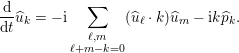 $$\begin{eqnarray}\frac{\text{d}}{\text{d}t}\widehat{u}_{k}=-\text{i}\mathop{\sum }_{\substack{ \ell ,m \\ \ell +m-k=0}}(\widehat{u}_{\ell }\cdot k)\widehat{u}_{m}-\text{i}k\widehat{p}_{k}.\end{eqnarray}$$
This is the Fourier space version of the Euler equations (1.3). It becomes evident that the pressure term  $-\text{i}k\widehat{p}_{k}$, which is parallel to
 $k$, serves as the orthogonal
 $L^{2}$ projection of the non-linear term
 $$\begin{eqnarray}-\text{i}\mathop{\sum }_{\substack{ \ell ,m \\ \ell +m-k=0}}(\widehat{u}_{\ell }\cdot k)\widehat{u}_{m}\end{eqnarray}$$
to the orthogonal complement of  $k$, thus keeping
 $u$ divergence-free.
For the coefficient  $\widehat{u}_{k}$ with
 $k=0$, equation (6.2) yields
 $(\text{d}/\text{d}t)\widehat{u}_{0}=0$. This corresponds to conservation of momentum. Using the Galilean invariance of the Euler equations, we can assume without loss of generality that
 $$\begin{eqnarray}\widehat{u}_{0}=\frac{1}{(2{\it\pi})^{d}}\int _{\mathbb{T}^{d}}u\,\text{d}x=0.\end{eqnarray}$$
To obtain a discretized approximation to system (6.2), we restrict our attention to the Fourier modes below some threshold  $N$. We thus consider divergence-free fields of the form
 $$\begin{eqnarray}u(x,t)=\mathop{\sum }_{|k|\leq N}u_{k}(t)\,\text{e}^{\text{i}k\cdot x},\end{eqnarray}$$
and use the  $N$-term Leray projection
 $$\begin{eqnarray}\mathbb{P}_{N}\biggl(\mathop{\sum }_{k\in \mathbb{Z}^{2}}\widehat{w}_{k}\,\text{e}^{\text{i}k\cdot x}\biggr):=\mathop{\sum }_{|k|\leq N}(\widehat{w}_{k}-k\widehat{q}_{k})\,\text{e}^{\text{i}k\cdot x},\quad \widehat{q}_{k}:=\frac{\widehat{w}_{k}\cdot k}{|k|^{2}}\end{eqnarray}$$
to ensure the divergence-free constraint  $(\widehat{w}_{k}-k\widehat{q}_{k})\bot k$. We can also add a small amount of numerical viscosity to ensure stability of the resulting scheme. This idea results in the following scheme. For initial data
 $u_{0}(x)$, we obtain an approximate solution
 $u_{N}(x,t)\approx u(x,t)$ by solving the finite-dimensional problem
 $$\begin{eqnarray}\begin{array}{@{}r@{}}\partial _{t}u_{N}+\mathbb{P}_{N}\,(u_{N}\cdot {\rm\nabla}u_{N})={\it\varepsilon}_{N}{\rm\Delta}u_{N},\\ u_{N}(x,0)=\mathbb{P}_{N}u_{0}(x).\end{array}\end{eqnarray}$$
In this scheme, the numerical diffusion coefficient  ${\it\varepsilon}_{N}>0$ depends on
 $N$ and goes to zero as
 $N\rightarrow \infty$.
A refined version of this basic scheme was introduced by Tadmor (Reference Tadmor1989). In this version we choose an integer  $m=m(N)\sim {\it\theta}N$ for some
 ${\it\theta}\in (0,1)$ which serves as a threshold between small and large Fourier modes. We apply a viscous regularization only to the large Fourier modes. With a judicious choice of
 ${\it\varepsilon}_{N}$ and
 $m(N)$, the resulting method can be shown to be spectrally accurate (see Tadmor Reference Tadmor1989, Bardos and Tadmor Reference Bardos and Tadmor2015, and Section 3.4 of Tadmor Reference Tadmor2012). We obtain the corresponding spectral viscosity approximation
 $$\begin{eqnarray}\begin{array}{@{}rcl@{}}\partial _{t}u_{N}+\mathbb{P}_{N}\,(u_{N}\cdot {\rm\nabla}u_{N})\; & =\; & {\it\varepsilon}_{N}{\rm\nabla}\cdot (\mathbb{Q}_{N}{\rm\nabla}u_{N}),\\ u_{N}(x,0)\; & =\; & \mathbb{P}_{N}u_{0}(x).\end{array}\end{eqnarray}$$
Here  $\mathbb{Q}_{N}$ denotes a smooth cut-off onto the higher modes,
 $|k|\geq {\it\theta}N$, for some
 ${\it\theta}<1$:
 $$\begin{eqnarray}\mathbb{Q}_{N}w(x):=\mathop{\sum }_{{\it\theta}N\leq |k|\leq N}{\it\sigma}\biggl(\frac{|k|}{N}\biggr)\widehat{w}_{k}\,\text{e}^{\text{i}k\cdot x},\quad {\it\sigma}(t)=(t-{\it\theta})_{+}^{2p}.\end{eqnarray}$$
The fully viscous spectral method (6.3) corresponds to the special choice of  ${\it\theta}=0$ and
 $p=0$. The application of spectral viscosity for simulations of three-dimensional Euler equations can be found in Karamanos and Karniadakis (Reference Karamanos and Karniadakis2000), Pasquetti (Reference Pasquetti2006) and Avrin and Xiao (Reference Avrin and Xiao2014).
Lanthaler and Mishra (Reference Lanthaler and Mishra2015) derived the following stability estimate.
Lemma 6.1 (stability).
If  $u_{N}$ is the solution of the semi-discrete system (6.4), then
 $$\begin{eqnarray}\displaystyle \frac{1}{2}\Vert u_{N}(t)\Vert _{L^{2}}^{2}+{\it\varepsilon}_{N}\int _{0}^{t}\Vert \mathbb{Q}_{N}{\rm\nabla}u_{N}(s)\Vert _{L^{2}}^{2}\,\text{d}s=\frac{1}{2}\Vert \mathbb{P}_{N}u_{0}\Vert _{L^{2}}^{2}\leq \frac{1}{2}\Vert u_{0}\Vert _{L^{2}}^{2}. & & \displaystyle\end{eqnarray}$$
In particular, we have  $\Vert u_{N}(t)\Vert _{L^{2}}\leq \Vert u_{0}\Vert _{L^{2}}$, independent of the choice of
 $N,m$ and
 ${\it\varepsilon}_{N}$.
The following consistency estimate was also proved in Lanthaler and Mishra (Reference Lanthaler and Mishra2015).
Lemma 6.2 (consistency).
If  $u_{N}$ is the solution of the semi-discrete system (6.4), then for all divergence-free test functions
 ${\it\varphi}$ in
 $C_{c}^{\infty }([0,T)\times \mathbb{T}^{d})$,
 $$\begin{eqnarray}\lim _{N\rightarrow \infty }\int _{\mathbb{R}_{+}}\int _{\mathbb{T}^{d}}\partial _{t}{\it\varphi}\cdot u_{N}+{\rm\nabla}{\it\varphi}:u_{N}\otimes u_{N}\,\text{d}x\,\text{d}t=0.\end{eqnarray}$$
Furthermore, we have uniform Lipschitz continuity
 $$\begin{eqnarray}u_{N}\in \text{Lip}([0,T];H^{-d/2-1}(\mathbb{T}^{d})).\end{eqnarray}$$
6.1.2 Approximation of measure-valued solutions
Next, we apply the numerical method described above to the FKMT algorithm. Relabelling  ${\rm\Delta}{\rightsquigarrow}N$, we let
 $\mathbf{S}_{t}^{N}u_{0}:=u_{N}$ denote the approximate spectral viscosity solution computed by (6.4), and apply this to Step 2 of Algorithm 4.1. The following convergence theorem for Algorithm 4.1 was proved in the recent paper by Lanthaler and Mishra (Reference Lanthaler and Mishra2015).
Theorem 6.3. Consider the approximate measure-valued solution  ${\it\nu}^{N}$ computed by Algorithm 4.1 using the spectral viscosity method (6.4) as the numerical solution operator
 $\mathbf{S}_{t}^{N}$. Assume that the (kinetic) energy of the initial Young measure
 ${\it\sigma}$ is finite, that is,
 $$\begin{eqnarray}\int _{\mathbb{T}^{d}}\langle {\it\sigma}_{x},|{\it\xi}|^{2}\rangle \,\text{d}x<\infty .\end{eqnarray}$$
Then  ${\it\nu}^{N}$ converges weak* (up to a subsequence) to an admissible measure-valued solution
 $({\it\nu},{\it\lambda},{\it\nu}^{\infty })$ of the incompressible Euler equations (1.3) with initial data
 ${\it\sigma}$.
The following theorem proves the analogous result for Algorithm 4.3 for atomic initial data.
Theorem 6.4. Let  $u_{0}\in L^{2}(\mathbb{T}^{d})$. Let
 ${\it\nu}^{N,{\it\varepsilon}}$ be the family of approximate measure-valued solutions constructed by Algorithm 4.3, with the spectral viscosity method (6.4) defining the numerical solution operator
 $\mathbf{S}_{t}^{N}$. Then there exists a subsequence
 $N_{n}\rightarrow \infty$,
 ${\it\varepsilon}_{n}\rightarrow 0$ such that
 $$\begin{eqnarray}{\it\nu}^{N_{n},{\it\varepsilon}_{n}}\overset{\ast }{\rightharpoonup }({\it\nu},{\it\lambda},{\it\nu}^{\infty })\quad \text{as }n\rightarrow \infty\end{eqnarray}$$
for an admissible measure-valued solution  $({\it\nu},{\it\lambda},{\it\nu}^{\infty })$ of the incompressible Euler equations (1.3) with atomic initial data
 $u_{0}$.
It was also shown by Lanthaler and Mishra (Reference Lanthaler and Mishra2015) that the Monte Carlo version (using Algorithm 4.4) also converges to an admissible measure-valued solution of the incompressible Euler equations (1.3).
6.2 A finite difference projection method for the incompressible Euler equations
Although spectral (viscosity) methods such as (6.4) can be highly efficient for periodic boundary conditions, it is not possible to use them when more complicated domains and different boundary conditions are required. In this context, finite difference projection methods, such as those developed by Chorin (Reference Chorin1968) (see Bell, Colella and Glaz Reference Bell, Colella and Glaz1989 for modern variants) are more promising. Here, we present a variant of the Chorin finite difference projection algorithm, considered in Leonardi and Mishra (Reference Leonardi and Mishra2016), which can be used to define the numerical solution operator in Step 2 of Algorithms 4.1 and 4.3.
6.2.1 The numerical method $\mathbf{S}_{t}^{h}$

For simplicity of the exposition, we restrict ourselves to the two-dimensional version of the incompressible Euler equations (1.3) and discretize the domain into Cartesian cells with mesh size  ${\rm\Delta}:=({\rm\Delta}x,{\rm\Delta}y)$. These two-dimensional cells,
 $$\begin{eqnarray}{\mathcal{C}}_{i,j}:=[x_{i-1/2},x_{i+1/2})\times [y_{j-1/2},y_{j+1/2}),\end{eqnarray}$$
are assumed to have similar mesh sizes, that is,  ${\rm\Delta}x=x_{i+1/2}-x_{i-1/2}$ and
 ${\rm\Delta}y=y_{j+1/2}-y_{j-1/2}$, such that
 ${\rm\Delta}y=ch,{\rm\Delta}x=h$ for some
 $c,h>0$. Let
 $$\begin{eqnarray}(x_{i},y_{j})=\biggl(\frac{x_{i-1/2}+x_{i+1/2}}{2},\frac{y_{j-1/2}+y_{j+1/2}}{2}\biggr)\end{eqnarray}$$
denote the midpoint of the cells. For a scalar function  ${\it\varphi}$ that is represented on the grid with its point values at
 $c$, we let
 $\text{grad}^{h}$ denote a cell-centred central, second-order discrete gradient operator defined as
 $$\begin{eqnarray}\text{grad}^{h}{\it\varphi}_{i,j}=\left(\begin{array}{@{}c@{}}\frac{{\it\varphi}_{i+1,j}-{\it\varphi}_{i-1,j}}{{\rm\Delta}x}\\ \frac{{\it\varphi}_{i,j+1}-{\it\varphi}_{i,j-1}}{{\rm\Delta}y}\end{array}\right)\!.\end{eqnarray}$$
We introduce the notation  ${\rm\Delta}^{h}$ for a standard five-point discrete Laplace operator:
 $$\begin{eqnarray}{\rm\Delta}^{h}{\it\varphi}_{i,j}=\frac{{\it\varphi}_{i+1,j}-2{\it\varphi}_{i,j}+{\it\varphi}_{i-1,j}}{{\rm\Delta}x}+\frac{{\it\varphi}_{i,j+1}-2{\it\varphi}_{i,j}+{\it\varphi}_{i,j-1}}{{\rm\Delta}y}.\end{eqnarray}$$
For a function  $u=(u_{1},u_{2})$ (the alias for the two-dimensional velocity field), represented on the grid by its point values at
 $(x_{i},y_{j})$, we define the discrete divergence operator
 $\text{div}^{h}$ as a cell-centred central divergence operator:
 $$\begin{eqnarray}\text{div}^{h}u_{i,j}=\frac{(u_{1})_{i+1,j}-(u_{1})_{i-1,j}}{{\rm\Delta}x}+\frac{(u_{2})_{i,j+1}-(u_{2})_{i,j-1}}{{\rm\Delta}y}.\end{eqnarray}$$
Equipped with the above notation, we define the following fully discrete fractional step predictor–corrector finite difference scheme for approximating the velocity field  $u_{i,j}\approx u(x_{i},y_{j})$:
 $$\begin{eqnarray}\displaystyle \frac{u^{\ast ,n+1}-u^{n}}{{\rm\Delta}t}+{\mathcal{C}}(u^{n},\bar{u}^{n+1/2}) & = & \displaystyle {\mathcal{D}}\bar{u}^{n+1/2},\end{eqnarray}$$
 $$\begin{eqnarray}\displaystyle \frac{u^{n+1}-u^{n}}{{\rm\Delta}t} & = & \displaystyle {\mathcal{P}}\biggl(\frac{u^{\ast ,n+1}-u^{n}}{{\rm\Delta}t}\biggr),\end{eqnarray}$$
 $$\begin{eqnarray}\displaystyle \text{grad}^{h}p^{n+1/2} & = & \displaystyle {\mathcal{Q}}\biggl(\frac{u^{n+1}-u^{n}}{{\rm\Delta}t}\biggr).\end{eqnarray}$$
(i) Time-averaged velocity. We use a time-averaged velocity  $\bar{u}^{n+1/2}:={\it\theta}u^{n}+(1-{\it\theta})u^{\ast ,n+1},{\it\theta}\in [0,1/2)$ in order to prove some essential stability properties. This time-averaged velocity is used in both the convective and numerical diffusion terms. It makes the convective step (6.7a) implicit.
(ii) Numerical diffusion operator  ${\mathcal{D}}$. We use Lax–Wendroff-type diffusion operators of the form
 $$\begin{eqnarray}\displaystyle {\mathcal{D}}u & = & \displaystyle \frac{\text{d}_{i+1/2,j}|\unicode[STIX]{x27E6}u_{1}\unicode[STIX]{x27E7}_{i+1/2,j}^{x}|^{k-1}\unicode[STIX]{x27E6}u_{1}\unicode[STIX]{x27E7}_{i+1/2,j}^{x}+d_{i-1/2,j}|\unicode[STIX]{x27E6}u_{1}\unicode[STIX]{x27E7}_{i-1/2,j}^{x}|^{k-1}\unicode[STIX]{x27E6}u_{1}\unicode[STIX]{x27E7}_{i-1/2,j}^{x}}{{\rm\Delta}x}\nonumber\\ \displaystyle & & \displaystyle +\frac{\text{d}_{i,j+1/2}|\unicode[STIX]{x27E6}u_{2}\unicode[STIX]{x27E7}_{i,j+1/2}^{y}|^{k-1}\unicode[STIX]{x27E6}u_{2}\unicode[STIX]{x27E7}_{i,j+1/2}^{y}+d_{i,j-1/2}|\unicode[STIX]{x27E6}u_{2}\unicode[STIX]{x27E7}_{i,j-1/2}^{y}|^{k-1}\unicode[STIX]{x27E6}u_{2}\unicode[STIX]{x27E7}_{i,j-1/2}^{y}}{{\rm\Delta}y},\nonumber\end{eqnarray}$$
expressed in terms of the respective jumps  $\unicode[STIX]{x27E6}a\unicode[STIX]{x27E7}^{x}:=a_{i+1,j}-a_{i,j}$ and
 $\unicode[STIX]{x27E6}a\unicode[STIX]{x27E7}^{y}:=a_{i,j+1}-a_{i,j}$, where
 $d_{{\it\alpha},{\it\beta}}$ are positive viscosity amplitudes and
 $k$ is an integer (
 $k=2$ being a common choice).
(iii) Projection operator  ${\mathcal{P}}$. We let
 ${\mathcal{P}}$ denote a discrete projection operator onto a discretely divergence-free vector space (i.e., such that
 $\text{div}^{h}u=0$) and
 ${\mathcal{Q}}=\text{I}-{\mathcal{P}}$ (the gradient, or irrotational, part of the vector field, where
 $\text{I}$ is the identity map). The discrete projection is implemented by setting
 ${\mathcal{P}}u:=u-\text{grad}^{h}({\rm\Delta}_{2}^{h})^{-1}\text{div}^{h}u$, where
 ${\rm\Delta}_{2}^{h}=\text{div}^{h}\text{grad}^{h}$ is a standard cell-centred five-point Laplacian acting on cell-centres in checkerboard formation:
 $$\begin{eqnarray}{\rm\Delta}_{2}^{h}{\it\varphi}_{i,j}=\frac{{\it\varphi}_{i+2,j}-2{\it\varphi}_{i,j}+{\it\varphi}_{i-2,j}}{4{\rm\Delta}x^{2}}+\frac{{\it\varphi}_{i,j+2}-2{\it\varphi}_{i,j}+{\it\varphi}_{i,j-2}}{4{\rm\Delta}y^{2}},\end{eqnarray}$$
for a grid function  ${\it\varphi}$.
(iv) The non-linear (convective) term  ${\mathcal{C}}$. The non-linear convective term is evaluated at two different discrete quantities, namely the ‘lagged’ velocity
 $u^{n}$ and the time-averaged
 $\bar{u}^{n+1/2}$. Moreover, we use an energy conservative (second-order, consistent) flux term:
 $$\begin{eqnarray}\displaystyle {\mathcal{C}}(u,v)_{i,j} & = & \displaystyle \frac{F^{x}(u_{i,j},~u_{i+1,j},~v_{i,j},~v_{i+1,j})-F^{x}(u_{i-1,j},~u_{i,j},~v_{i-1,j},~v_{i,j})}{{\rm\Delta}x}\nonumber\\ \displaystyle & & \displaystyle +\frac{F^{y}(u_{i,j},~u_{i,j+1},~v_{i,j},~v_{i,j+1})-F^{y}(u_{i,j-1},~u_{i,j},~v_{i,j-1},~v_{i,j})}{{\rm\Delta}y}.\nonumber\end{eqnarray}$$
We employ the following numerical fluxes:
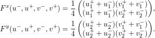 $$\begin{eqnarray}\displaystyle F^{x}(u^{-},u^{+},v^{-},v^{+}) & = & \displaystyle \frac{1}{4}\left(\begin{array}{@{}c@{}}(u_{1}^{+}+u_{1}^{-})(v_{1}^{+}+v_{1}^{-})\\ (u_{1}^{+}+u_{1}^{-})(v_{2}^{+}+v_{2}^{-})\end{array}\right)\!,\quad \nonumber\\ \displaystyle F^{y}(u^{-},u^{+},v^{-},v^{+}) & = & \displaystyle \frac{1}{4}\left(\begin{array}{@{}c@{}}(u_{2}^{+}+u_{2}^{-})(v_{1}^{+}+v_{1}^{-})\\ (u_{2}^{+}+u_{2}^{-})(v_{2}^{+}+v_{2}^{-})\end{array}\right)\!.\nonumber\end{eqnarray}$$
6.2.2 Approximation of measure-valued solutions
We apply the same Algorithm 4.1, but this time with the projection evolution  $\mathbf{S}_{t}^{h}$ replacing
 $\mathbf{S}_{t}^{{\rm\Delta}}$ in Step 2. The following convergence result is proved in Leonardi and Mishra (Reference Leonardi and Mishra2016).
Theorem 6.5. Consider the approximate measure-valued solution  ${\it\nu}^{h}$ generated by Algorithm 4.1 using the finite difference projection method (6.7) as the numerical solution operator
 $\mathbf{S}_{t}^{h}$. Assume that the (kinetic) energy of the initial Young measure
 ${\it\sigma}$ is finite, that is,
 $$\begin{eqnarray}\int _{\mathbb{T}^{n}}\langle {\it\sigma}_{x},|{\it\xi}|^{2}\rangle \,\text{d}x<\infty .\end{eqnarray}$$
Then  ${\it\nu}^{h}$ converges weak* (up to a subsequence) to an admissible measure-valued solution
 $({\it\nu},{\it\lambda},{\it\nu}^{\infty })$ of the incompressible Euler equations (1.3) with initial data
 ${\it\sigma}$.
The proof is based on several properties of the scheme (6.7), such as the equivalence between the conservative and convective forms of the scheme,  $L^{2}$ stability bounds and suitable weak BV estimates. We refer the reader to Leonardi and Mishra (Reference Leonardi and Mishra2016) for further details. Similarly, one can prove convergence of Algorithm 4.3 for computing admissible measure-valued solutions of (1.3) with atomic initial data.
7 Numerical experiments: compressible Euler equations
In this and the next section we will present various numerical experiments to illustrate the convergence and performance of Algorithms 4.1 and 4.3 in computing admissible measure-valued solutions of systems of conservation laws and the incompressible Euler equations.
We will focus on the prototype for multi-dimensional systems of conservation laws (2.1), the two-dimensional version of the compressible Euler equations (1.1):
 $$\begin{eqnarray}\frac{\partial }{\partial t}\left(\begin{array}{@{}c@{}}{\it\rho}\\ {\it\rho}v_{1}\\ {\it\rho}v_{2}\\ E\end{array}\right)+\frac{\partial }{\partial x_{1}}\left(\begin{array}{@{}c@{}}{\it\rho}v_{1}\\ {\it\rho}(v_{1})^{2}+p\\ {\it\rho}v_{1}v_{2}\\ (E+p)v_{1}\end{array}\right)+\frac{\partial }{\partial x_{2}}\left(\begin{array}{@{}c@{}}{\it\rho}v_{2}\\ {\it\rho}v_{1}v_{2}\\ {\it\rho}(v_{2})^{2}+p\\ (E+p)v_{2}\end{array}\right)=0.\end{eqnarray}$$
Here, the density  ${\it\rho}$, velocity field
 $(v_{1},v_{2})$, pressure
 $p$ and total energy
 $E$ are related by the equation of state
 $$\begin{eqnarray}E=\frac{p}{{\it\gamma}-1}+\frac{{\it\rho}((v_{1})^{2}+(v_{2})^{2})}{2},\end{eqnarray}$$
with adiabatic constant  ${\it\gamma}=1.4$. The relevant entropy pair
 $({\it\eta},q)$ is given in terms of the thermodynamic entropy
 $s:=\log (p{\it\rho}^{-{\it\gamma}})$,
 $$\begin{eqnarray}{\it\eta}=\frac{-{\it\rho}s}{{\it\gamma}-1},\quad q\equiv (q^{1},q^{2})=(v_{1}{\it\eta},v_{2}{\it\eta}).\end{eqnarray}$$
7.1 The Richtmyer–Meshkov problem
We consider the two-dimensional Euler equations (7.1) in the computational domain  $x\in [0,1]^{2}$ with periodic boundary conditions and with initial data
 $$\begin{eqnarray}\displaystyle p(x)=\left\{\begin{array}{@{}ll@{}}20\quad & \text{if }r<0.1,\\ 1\quad & \text{otherwise,}\end{array}\right.\quad {\it\rho}(x)=\left\{\begin{array}{@{}ll@{}}2\quad & \text{if }r<I({\it\omega};x),\\ 1\quad & \text{otherwise,}\end{array}\right.\quad v_{1}=v_{2}=0, & & \displaystyle\end{eqnarray}$$
where  $r:=|x-(0.5,0.5)|$ denotes the distance to the centre of the domain. The radial density interface
 $I({\it\omega};x)=0.25+{\it\varepsilon}Y({\it\omega};{\it\phi}(x))$ is perturbed with
 $$\begin{eqnarray}Y({\it\omega};{\it\phi})=\mathop{\sum }_{n=1}^{K}a^{n}({\it\omega})\cos ({\it\phi}+b^{n}({\it\omega})),\end{eqnarray}$$
where  ${\it\phi}(x)=\arccos ((x_{1}-1/2)/r)$ and
 $$\begin{eqnarray}a_{j}^{n}=a_{j}^{n}({\it\omega})\in [0,1],\quad b_{j}^{n}=b_{j}^{n}({\it\omega})\in [-{\it\pi},{\it\pi}],\quad i=1,2,~n=1,\ldots ,K,\end{eqnarray}$$
are uniformly distributed random numbers. The coefficients  $a_{j}^{n}$ have been normalized such that
 $$\begin{eqnarray}\mathop{\sum }_{n=1}^{K}a_{j}^{n}=1,\end{eqnarray}$$
to guarantee that  $|I_{j}({\it\omega};x)-J_{j}|\leq {\it\varepsilon}$ for
 $j=1,2$. We set
 $K=10$.
We remark that the above initial data can be written as in Step 1 of Algorithm 4.3 with an appropriate random field  $X$. Thus, the initial data can be thought of as a small perturbation of the spherically symmetric initial data obtained by letting
 $I\equiv 0.25$ in (7.2), and we can apply the procedure outlined in Algorithm 4.3 to compute an approximate measure-valued solution to these unperturbed initial data.
The results presented here were first shown in Fjordholm et al. (Reference Fjordholm, Käppeli, Mishra and Tadmor2016a).
7.1.1 Single realization
As a first test, we fix  ${\it\omega}\in {\rm\Omega}$ and compute approximate solutions using the second-order accurate Monte Carlo limiter and HLLC flux-based finite volume scheme of Käppeli et al. (Reference Käppeli, Whitehouse, Scheidegger, Pen and Liebendörfer2011). The computed density, at time
 $T=4$, on a sequence of successively refined grids ranging from
 $128^{2}$ to
 $1024^{2}$, is shown in Figure 1.2. As stated in the Introduction, the solution is quite complex at this time as the leading shock wave has exited the domain but has re-entered from the corners on account of the periodic boundary conditions. Furthermore, this re-entry shock wave interacts with and strongly perturbs the interface, forming a very complex region of small-scale eddy-like structures. As seen in Figure 1.2, there seems to be no convergence as the mesh is refined. This lack of convergence is quantified in Figure 1.3, where we present differences in
 $L^{1}$ for successive mesh resolutions (1.2), and we see that the approximate solutions for a single sample do not even form a Cauchy sequence, let alone converge.
The mean density for the Richtmyer–Meshkov problem with initial data (7.2) for different grid resolutions at time  $t=4$. All results are obtained with
 $400$ Monte Carlo samples.
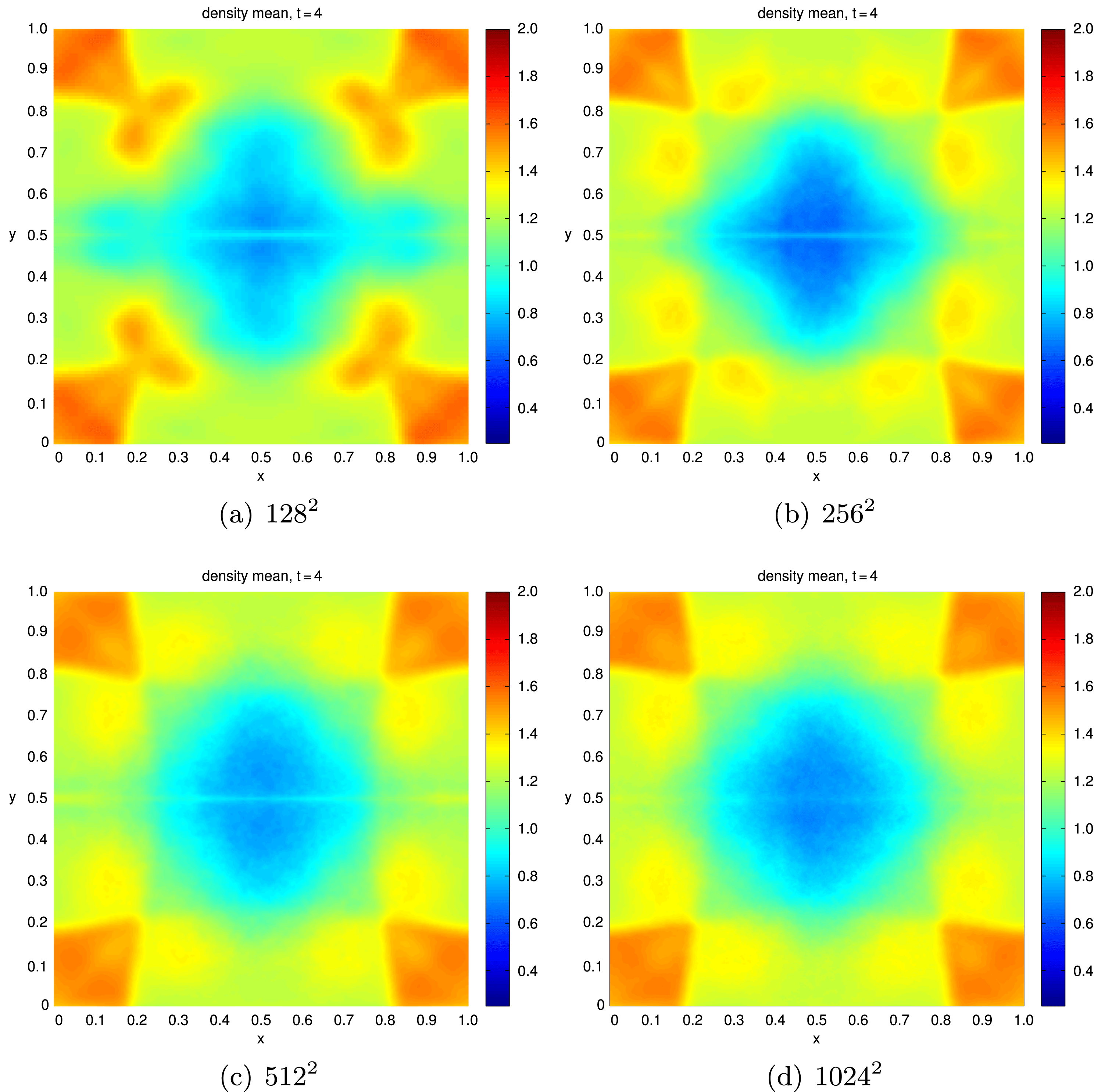
7.1.2 Ensemble of solutions
Next, we apply Algorithm 4.3 using the Monte Carlo approximation of Algorithm 4.4, with the perturbed initial data (7.2). We use  $M=400$ Monte Carlo samples and compute up to
 $t=4$ using grid resolutions from
 $128^{2}$ up to
 $1024^{2}$ grid points.
In Figure 7.1, for each grid resolution  ${\rm\Delta}x$ we plot the mean of the density variable:
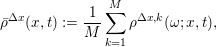 $$\begin{eqnarray}\bar{{\it\rho}}^{{\rm\Delta}x}(x,t):=\frac{1}{M}\mathop{\sum }_{k=1}^{M}{\it\rho}^{{\rm\Delta}x,k}({\it\omega};x,t),\end{eqnarray}$$
where  ${\it\rho}^{{\rm\Delta}x,k}({\it\omega})$ is the mass density of each individual Monte Carlo sample. We observe that small-scale features are averaged out in the mean, and only large-scale structures, such as the strong re-entrant shocks (recall the periodic boundary conditions) and mixing regions, are retained through the averaging process. The figure indicates that, unlike the individual samples shown in Figure 1.2, the mean converges as the mesh is refined. This convergence is quantified in Figure 7.2(a), where we plot the difference in the mean density for successive resolutions:
 $$\begin{eqnarray}\Vert \bar{{\it\rho}}^{{\rm\Delta}x}(\cdot ,t)-\bar{{\it\rho}}^{{\rm\Delta}x/2}(\cdot ,t)\Vert _{L^{1}}.\end{eqnarray}$$
The figure indicates that this quantity goes to zero, so the approximate means form a Cauchy sequence and hence converge.


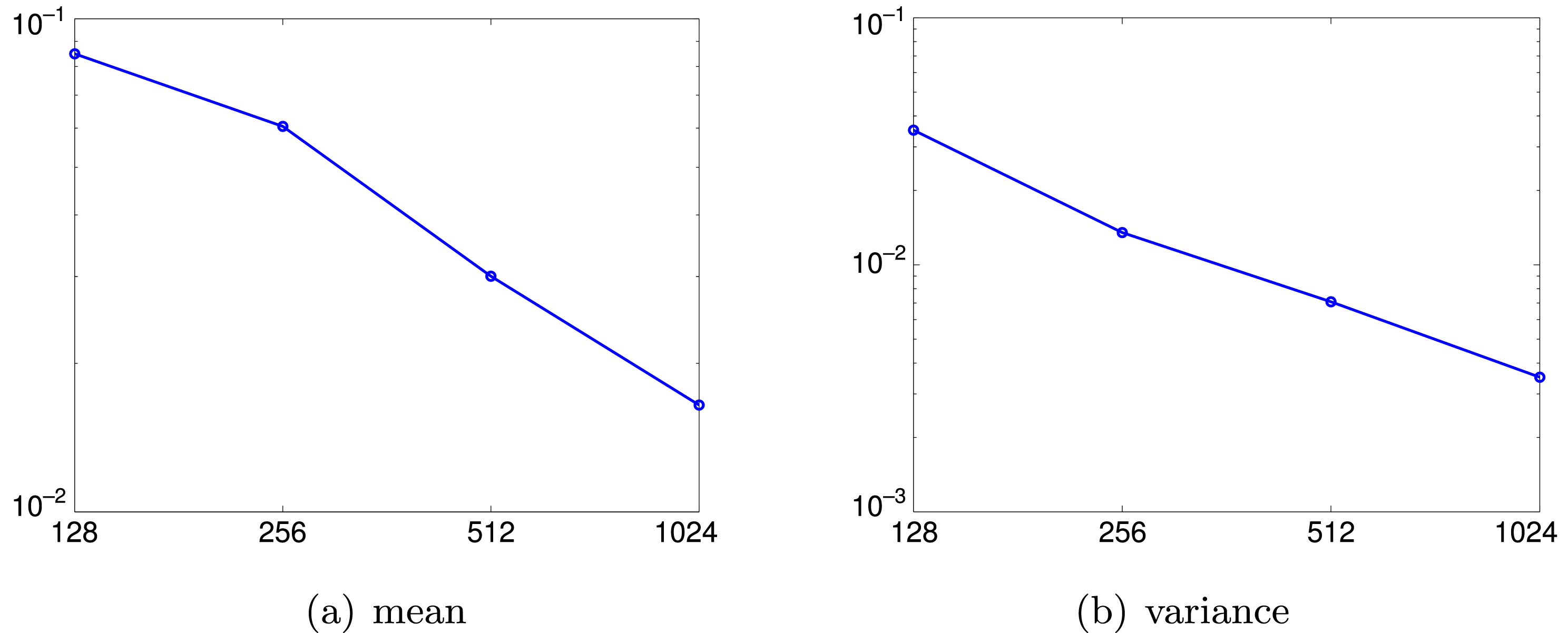
Figure 7.3 shows the variance of the mass density:
 $$\begin{eqnarray}\text{Var}({\it\rho}^{{\rm\Delta}x})(x,t):=\frac{1}{M}\mathop{\sum }_{k=1}^{M}({\it\rho}^{{\rm\Delta}x,k}({\it\omega};x,t)-\bar{{\it\rho}}^{{\rm\Delta}x}({\it\omega};x,t))^{2}.\end{eqnarray}$$
Variance of the density with initial data (7.2) for different grid resolutions at time  $t=4$. All results are obtained with
 $400$ Monte Carlo samples.
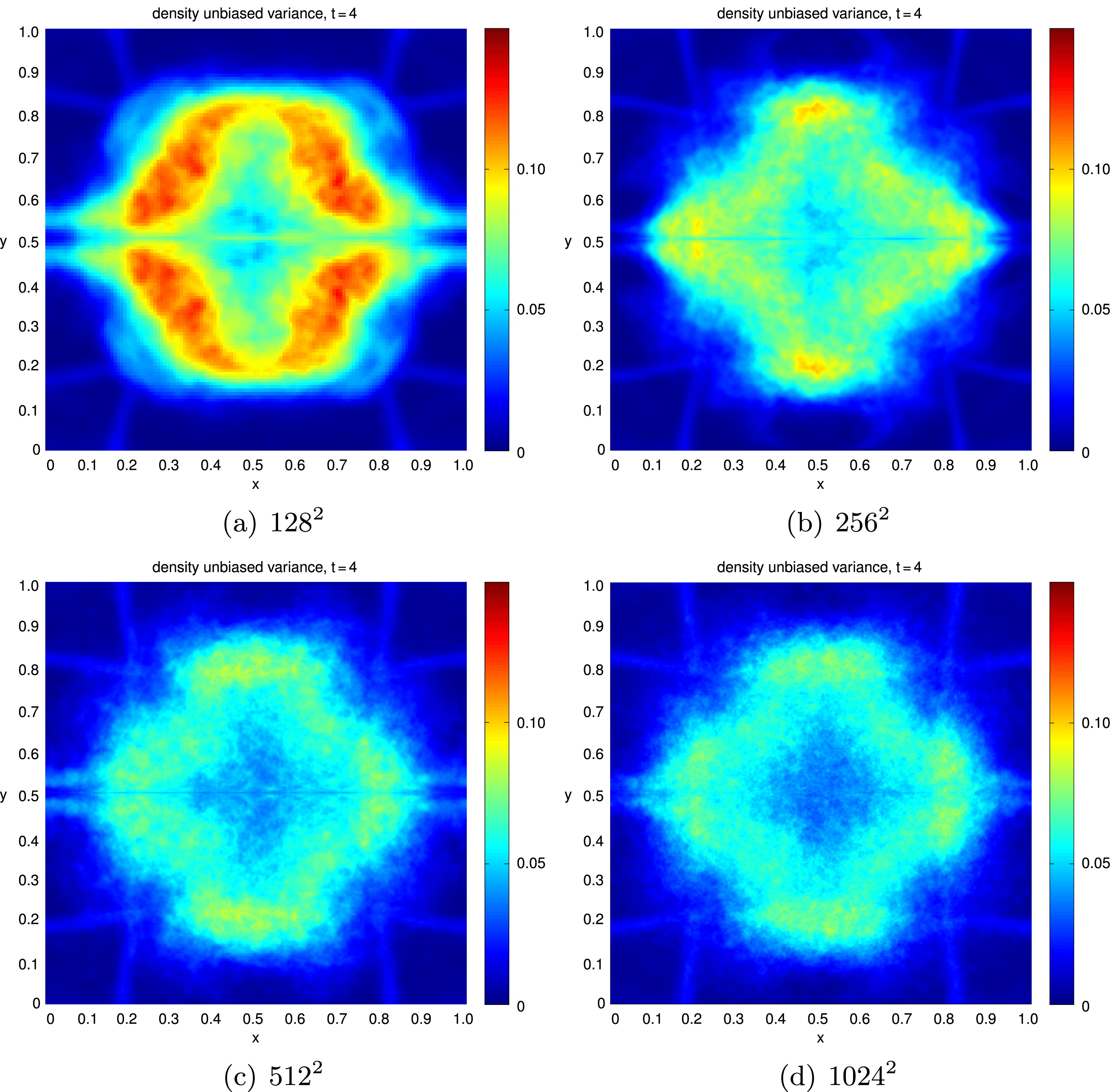
As in Figure 7.1, the variances of the approximate Young measures seem to converge as the mesh is refined. This is again quantified in Figure 7.2(b), where the  $L^{1}$ differences of the variances at successive mesh resolutions are plotted. Note from Figure 7.3 that the variance is concentrated at the shocks, and even more so in the mixing layer around the original interface.
7.2 The Kelvin–Helmholtz problem
Approximate density at time  $T=2$, computed with the TeCNO2 scheme for a single sample with initial data (7.6) for different initial perturbation amplitudes
 ${\it\varepsilon}$ on a grid of
 $1024^{2}$ points.
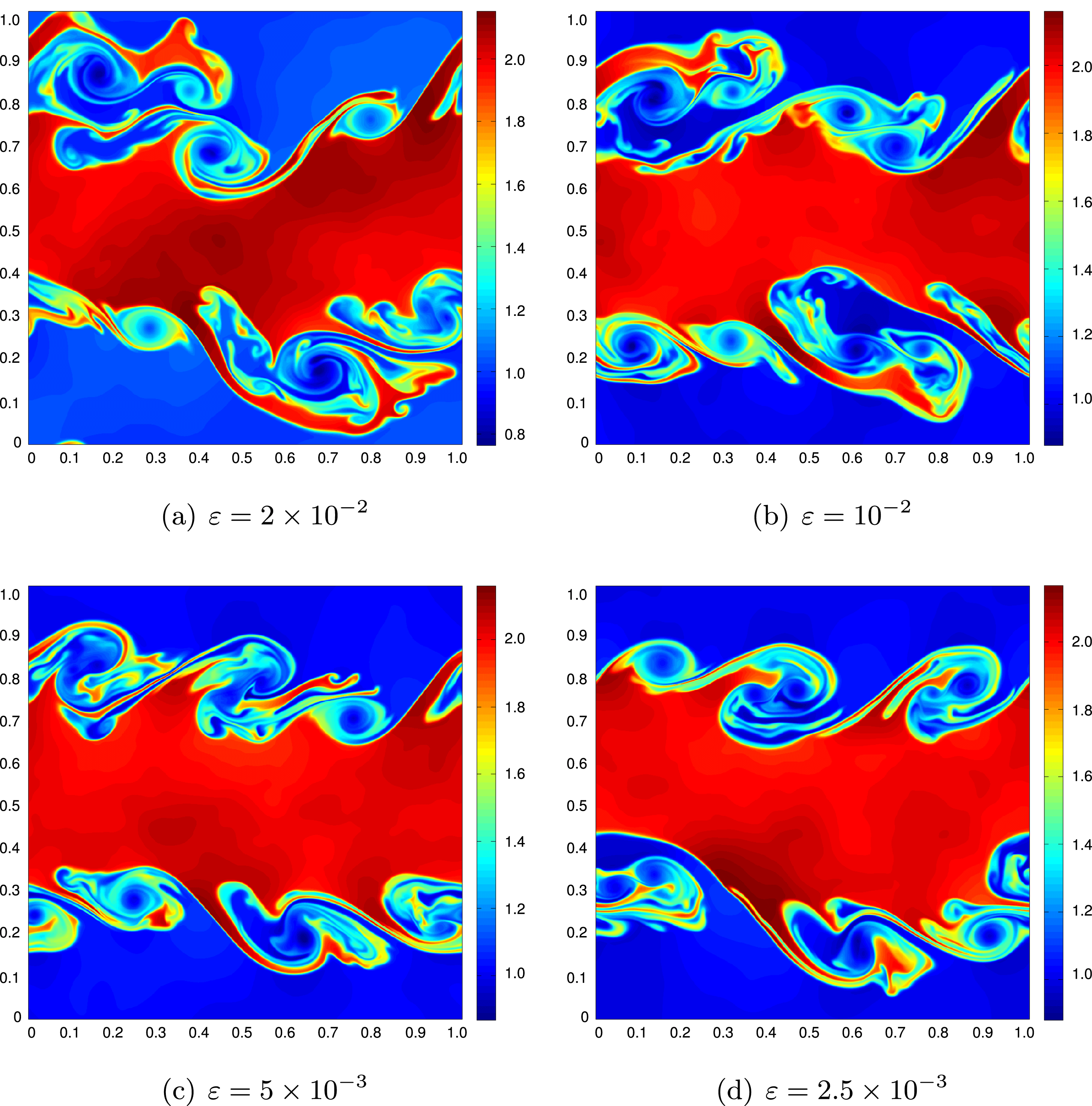
We consider the two-dimensional compressible Euler equations of gas dynamics (7.1) with initial data
 $$\begin{eqnarray}u_{0}(x)=\left\{\begin{array}{@{}ll@{}}u_{A}\quad & \text{if }J_{1}<x_{2}<J_{2},\\ u_{B}\quad & \text{if }\text{otherwise},\end{array}\right.\quad x\in [0,1]^{2},\end{eqnarray}$$
with  ${\it\rho}_{A}=2$,
 ${\it\rho}_{B}=1$,
 $(v_{1})_{A}=-0.5$,
 $(v_{1})_{B}=0.5$,
 $(v_{2})_{A}=(v_{2})_{B}=0$ and
 $p_{A}=p_{B}=2.5$. The interface is specified by setting
 $J_{1}=0.25$ and
 $J_{2}=0.75$. We use periodic boundary conditions on the computational domain
 $x\in [0,1]^{2}$.
Note that the initial data (7.6) are a steady-state solution of the Euler equations (7.1). Our aim is to compute a dissipative measure-valued solution of (7.1) with atomic initial data (7.6). To this end, we will employ Algorithm 4.3, adding a random perturbation of the initial data. We follow Fjordholm et al. (Reference Fjordholm, Käppeli, Mishra and Tadmor2016a) and randomly perturb the interfaces in (7.6) by setting
 $$\begin{eqnarray}u_{0}(x,{\it\omega})=\left\{\begin{array}{@{}ll@{}}u_{A}\quad & \text{if }I_{1}({\it\omega};x)<x_{2}<I_{2}({\it\omega};x),\\ u_{B}\quad & \text{if }\text{otherwise},\end{array}\right.\quad x\in [0,1]^{2},\end{eqnarray}$$
where
 $$\begin{eqnarray}I_{j}({\it\omega};x):=J_{j}+{\it\varepsilon}Y_{j}({\it\omega};x),\quad j=1,2,\end{eqnarray}$$
which are small perturbations around  $J_{1}=0.25$ and
 $J_{2}=0.75$, respectively, and
 $$\begin{eqnarray}Y_{j}({\it\omega};x)=\mathop{\sum }_{n=1}^{K}a_{j}^{n}({\it\omega})\cos (b_{j}^{n}({\it\omega})+2n{\it\pi}x_{1}),\quad j=1,2.\end{eqnarray}$$
Here,
 $$\begin{eqnarray}a_{j}^{n}=a_{j}^{n}({\it\omega})\in [0,1],\quad b_{j}^{n}=b_{j}^{n}({\it\omega})\in [-{\it\pi},{\it\pi}],\quad i=1,2,~n=1,\ldots ,K,\end{eqnarray}$$
are uniformly distributed random numbers. The coefficients  $a_{j}^{n}$ have been normalized such that
 $$\begin{eqnarray}\mathop{\sum }_{n=1}^{K}a_{j}^{n}=1,\end{eqnarray}$$
to guarantee that  $|I_{j}({\it\omega};x)-J_{j}|\leq {\it\varepsilon}$ for
 $j=1,2$. We set
 $K=10$.
Observe that by making  ${\it\varepsilon}$ small, this
 ${\it\omega}$-ensemble of initial data lies inside a small ball centred at
 $u_{0}$. Indeed, it is readily checked that measured in, say, the
 $L^{p}([0,1]^{2})$ norm, every sample
 $u_{0}({\it\omega};\cdot )$ is
 $O({\it\varepsilon}^{1/p})$ away from the unperturbed steady state (7.6).
The Cauchy rates ( $L^{1}$ difference for successively reduced
 ${\it\varepsilon}$) for the density at
 $t=2$ (
 $y$-axis), versus different values of the perturbation parameter
 ${\it\varepsilon}$ (
 $x$-axis).
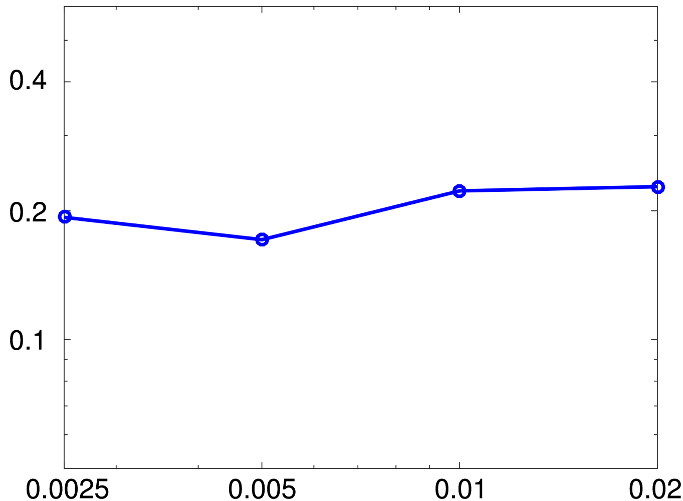
The lack of convergence with mesh refinement for single realizations has already been reported in Figures 6.2 and 6.3 of Fjordholm et al. (Reference Fjordholm, Käppeli, Mishra and Tadmor2016a). On the other hand, Figure 6.4 (resp. Figure 6.6) of Fjordholm et al. (Reference Fjordholm, Käppeli, Mishra and Tadmor2016a) demonstrated that statistical quantities of interest such as the mean and variance, when computed with Algorithm 4.1 (for any fixed value of  ${\it\varepsilon}$), converge when the mesh is refined. Moreover, convergence with respect to a Wasserstein-type metric was also observed (Figures 6.7 and 6.8 of Fjordholm et al. Reference Fjordholm, Käppeli, Mishra and Tadmor2016a).
7.2.1 Convergence as ${\it\varepsilon}\rightarrow 0$

Here we demonstrate the convergence of Algorithm 4.3. First, observe that the perturbed initial data (7.7) converge (in any reasonable metric) to the initial data (7.6) as  ${\it\varepsilon}\rightarrow 0$. Following Algorithm 4.3, we wish to study the limit behaviour of approximate solutions
 ${\it\nu}^{{\rm\Delta}x,{\it\varepsilon}}$ as
 ${\it\varepsilon}\rightarrow 0$. To this end, we compute approximate solutions using the TeCNO2 scheme (see Fjordholm et al. Reference Fjordholm, Mishra and Tadmor2012) at a very fine mesh resolution of
 $1024^{2}$ points for different values of
 ${\it\varepsilon}$.
Approximate sample means of the density for the Kelvin–Helmholtz problem (7.6) at time  $t=2$ and different values of perturbation parameter
 ${\it\varepsilon}$. All the computations are on a grid of
 $1024^{2}$ mesh points and
 $400$ Monte Carlo samples.
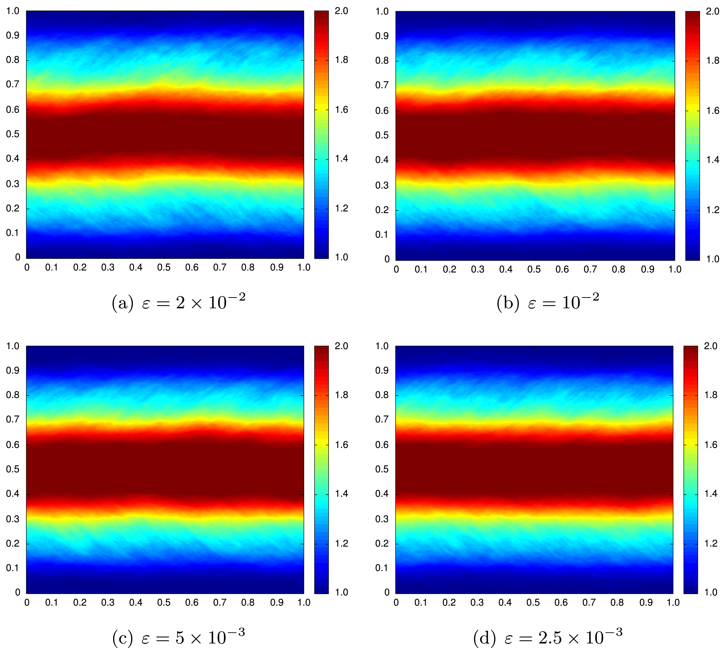
Results for a single sample at time  $t=2$ for different values of
 ${\it\varepsilon}$ are presented in Figure 7.4. The figures indicate that there is no convergence as
 ${\it\varepsilon}\rightarrow 0$. The spread of the mixing region seems to remain large even when the perturbation parameter is reduced. This lack of convergence is further quantified in Figure 7.5, where we plot the
 $L^{1}$ difference of the approximate density for successively reduced values of
 ${\it\varepsilon}$. This difference remains large even when
 ${\it\varepsilon}$ is reduced by an order of magnitude.
Next, we apply Algorithm 4.3 using the Monte Carlo approximation of Algorithm 4.4, with the perturbed initial data (7.7). We use  $M=400$ Monte Carlo samples and compute up to
 $t=2$ on a fixed grid resolution of
 $1024^{2}$ points, using different values of the perturbation parameter
 ${\it\varepsilon}$. The mean of the mass density (7.4) is plotted in Figure 7.6. The figure clearly shows convergence as
 ${\it\varepsilon}\rightarrow 0$, to a limit different from the steady-state solution (7.6). This convergence of the mean with respect to decaying
 ${\it\varepsilon}$ is quantified in Figure 7.7(a), where we compute the
 $L^{1}$ difference (7.5) of the mean for successive values of
 ${\it\varepsilon}$. We observe that the approximations of the mean form a Cauchy sequence, and hence converge.
Cauchy rates for the sample mean and the sample variance of the density ( $y$-axis) for the Kelvin–Helmholtz problem (7.6) for different values of
 ${\it\varepsilon}$ (
 $x$-axis). All the computations are on a grid of
 $1024^{2}$ mesh points and
 $400$ Monte Carlo samples.
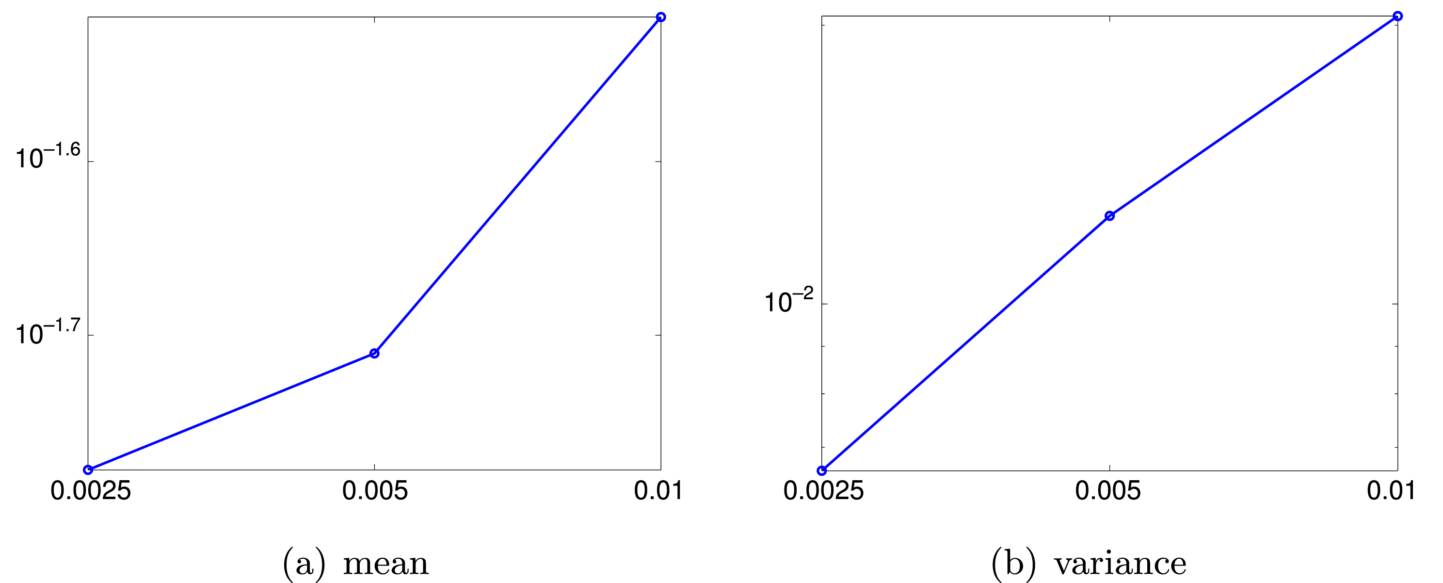
Similar computations of the variance for different values of  ${\it\varepsilon}$ are presented in Figures 7.8 and 7.7(b). These figures clearly show convergence of variance as
 ${\it\varepsilon}\rightarrow 0$. Moreover, Figure 7.8 clearly indicates that in the
 ${\it\varepsilon}\rightarrow 0$ limit, the limit variance is non-zero. This strongly suggests that dissipative measure-valued solution can be non-atomic, even for atomic initial data. These results are consistent with the claims of Theorem 5.5.
Approximate sample variances of the density for the Kelvin–Helmholtz instability at time  $t=2$ and different values of perturbation parameter
 ${\it\varepsilon}$. All the computations are on a grid of
 $1024^{2}$ mesh points and
 $400$ Monte Carlo samples.
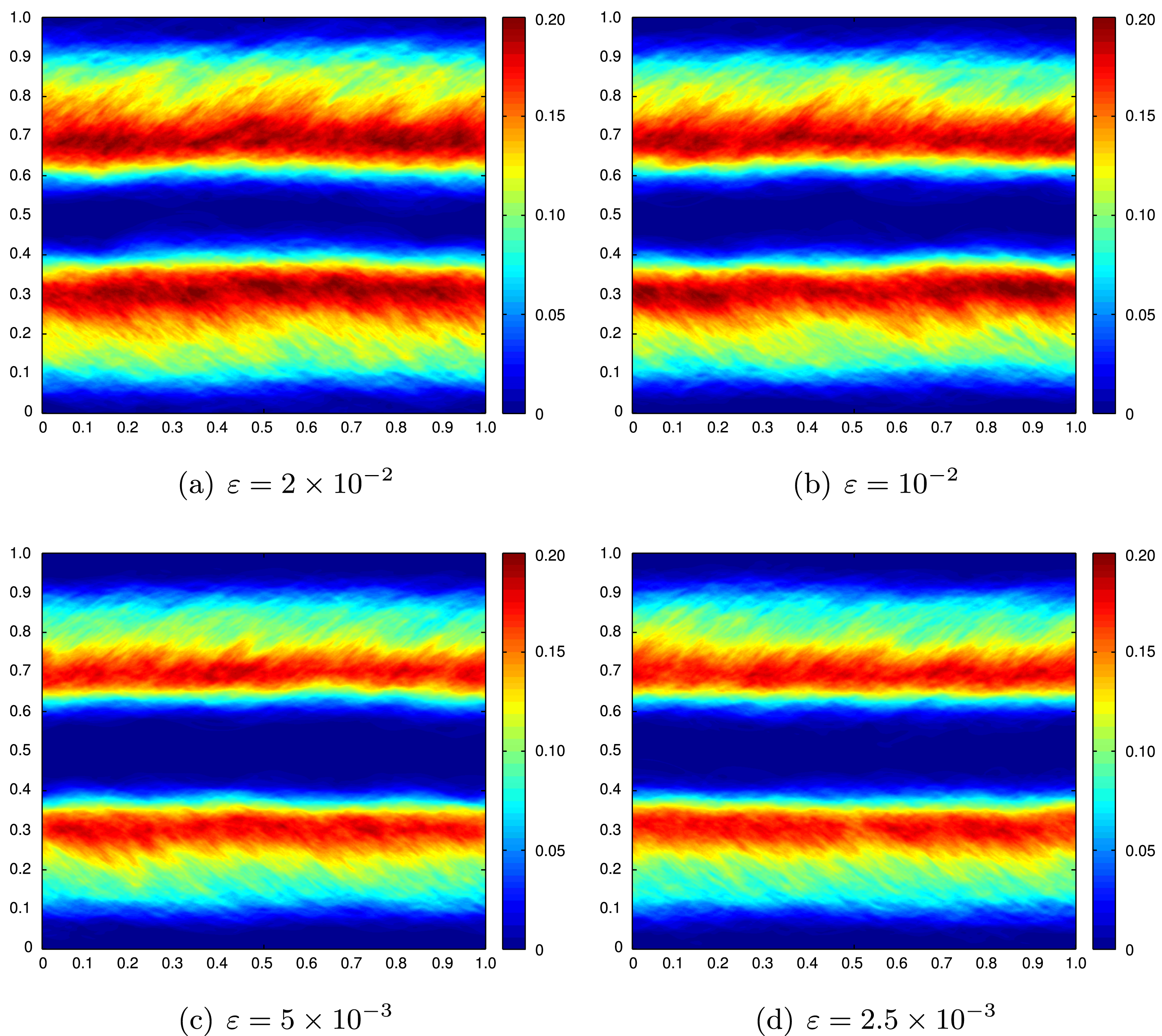
To further demonstrate the non-atomicity of the resulting measure-valued solution, we have plotted the probability density functions (PDFs), approximated by empirical histograms, for the mass density at the points  $x=(0.5,0.7)$ and
 $x=(0.5,0.8)$ in Figure 7.9. We see that the initial unit mass centred at
 ${\it\rho}=2$ (
 ${\it\rho}=1$, respectively) at
 $t=0$ is smeared out over time, and at
 $t=2$ the mass has spread out over a range of values of
 ${\it\rho}$ between 1 and 2.
Figure 7.10 shows the same quantities, but for a fixed time  $t=2$, over a series of meshes. Although a certain amount of noise seems to persist on the finer meshes – most likely due to the low number of Monte Carlo samples – the probability density functions seem to converge with mesh refinement.
Time evolution of the approximate PDF for density  ${\it\rho}$ at the points
 $x=(0.5,0.7)$ (a–e) and
 $x=(0.5,0.8)$ (f–j) on a grid of
 $1024^{2}$ mesh points.
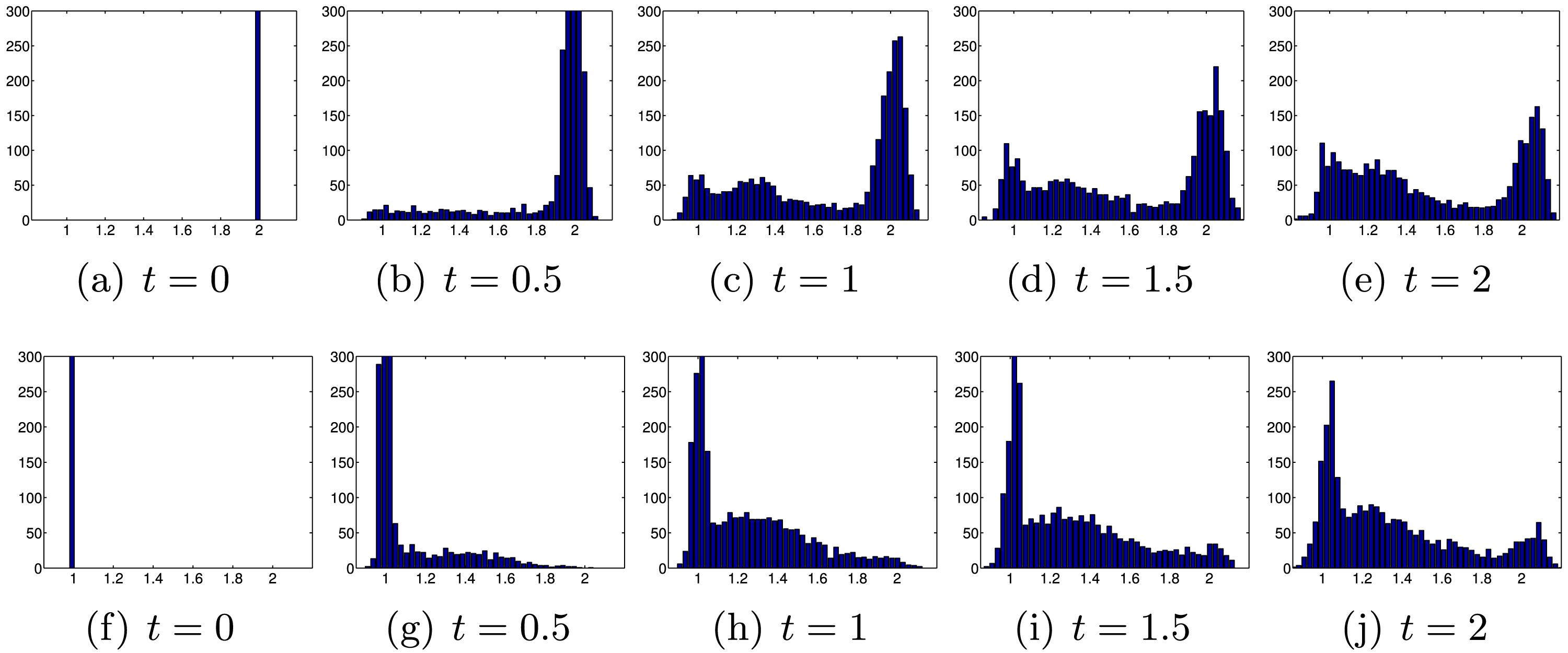
The approximate PDF for density  ${\it\rho}$ at the points
 $x=(0.5,0.7)$ (a–d) and
 $x=(0.5,0.8)$ (e–h) on a series of meshes.
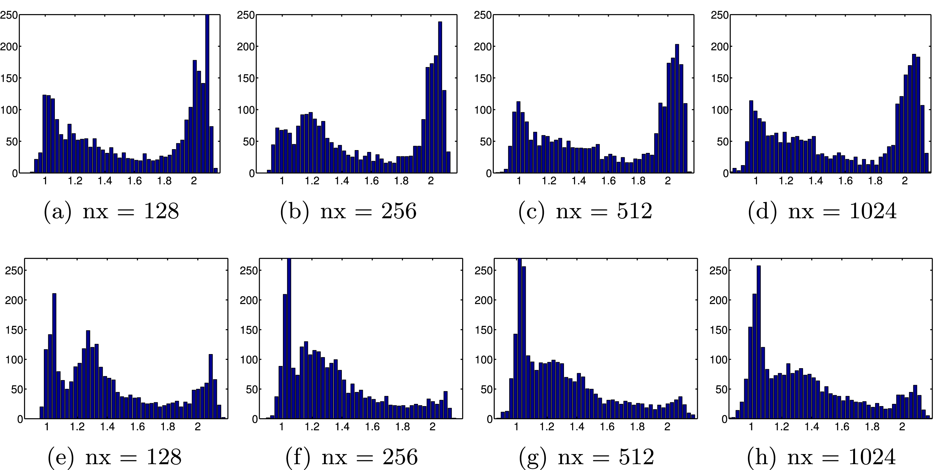
8 Numerical experiments: incompressible Euler equations
In this section we will consider the two-dimensional version of the incompressible Euler equations (1.3) and present a numerical experiment to illustrate Algorithms 4.1 and 4.3 for computing an admissible measure-valued solution.
8.1 Flat vortex sheet
We consider (1.3) in two dimensions with initial data
 $$\begin{eqnarray}u_{0}(x)=\left\{\begin{array}{@{}ll@{}}(-1,0)\quad & \text{if }\;{\it\pi}/2<x_{2}<3{\it\pi}/2,\\ (1,0)\quad & \text{otherwise,}\end{array}\right.\end{eqnarray}$$
on a periodic domain  $x\in [0,2{\it\pi}]^{2}$. The initial vorticity in this case is a bounded measure concentrated on the sets
 $x_{2}={\it\pi}/2$ and
 $x_{2}=3{\it\pi}/2$. It is straightforward to check that the initial data for the flat vortex sheet (8.1) is a steady-state weak solution of the two-dimensional Euler equations. However, this datum also belongs to the class of wild initial data in the sense of Székelyhidi (Reference Székelyhidi2011). Thus, infinitely many admissible weak solutions with this initial datum can be constructed, as was done in Székelyhidi (Reference Székelyhidi2011).
Our objective is to compute an (admissible) measure-valued solution for these atomic initial data by employing Algorithm 4.3. To this end, we mollify the initial data  $v_{0}$ to obtain a smooth approximation
 $u_{0}^{{\it\rho}}=({\it\pi}_{1}u_{0}^{{\it\rho}},{\it\pi}_{2}u_{0}^{{\it\rho}})$ of (8.1). This guarantees the existence of a smooth solution. Specifically, we used
 $$\begin{eqnarray}{\it\pi}_{1}u_{0}^{{\it\rho}}(x)=\left\{\begin{array}{@{}ll@{}}\tanh \biggl({\displaystyle \frac{x_{2}-{\it\pi}/2}{{\it\rho}}}\biggr)\quad & \text{if }x_{2}\leq {\it\pi},\\ \tanh \biggl({\displaystyle \frac{3{\it\pi}/2-x_{2}}{{\it\rho}}}\biggr)\quad & \text{if }x_{2}>{\it\pi},\end{array}\right.\quad {\it\pi}_{2}u_{0}^{{\it\rho}}(x)=0.\end{eqnarray}$$
with a small parameter  ${\it\rho}$. The parameter
 ${\it\rho}$ controls the sharpness of the transition from
 $-1$ to
 $+1$ across the interfaces. A small value of
 ${\it\rho}$ corresponds to a very sharp transition.
Perturbed initial data with  ${\it\varepsilon}=0.0512$,
 ${\it\rho}=0.001$.
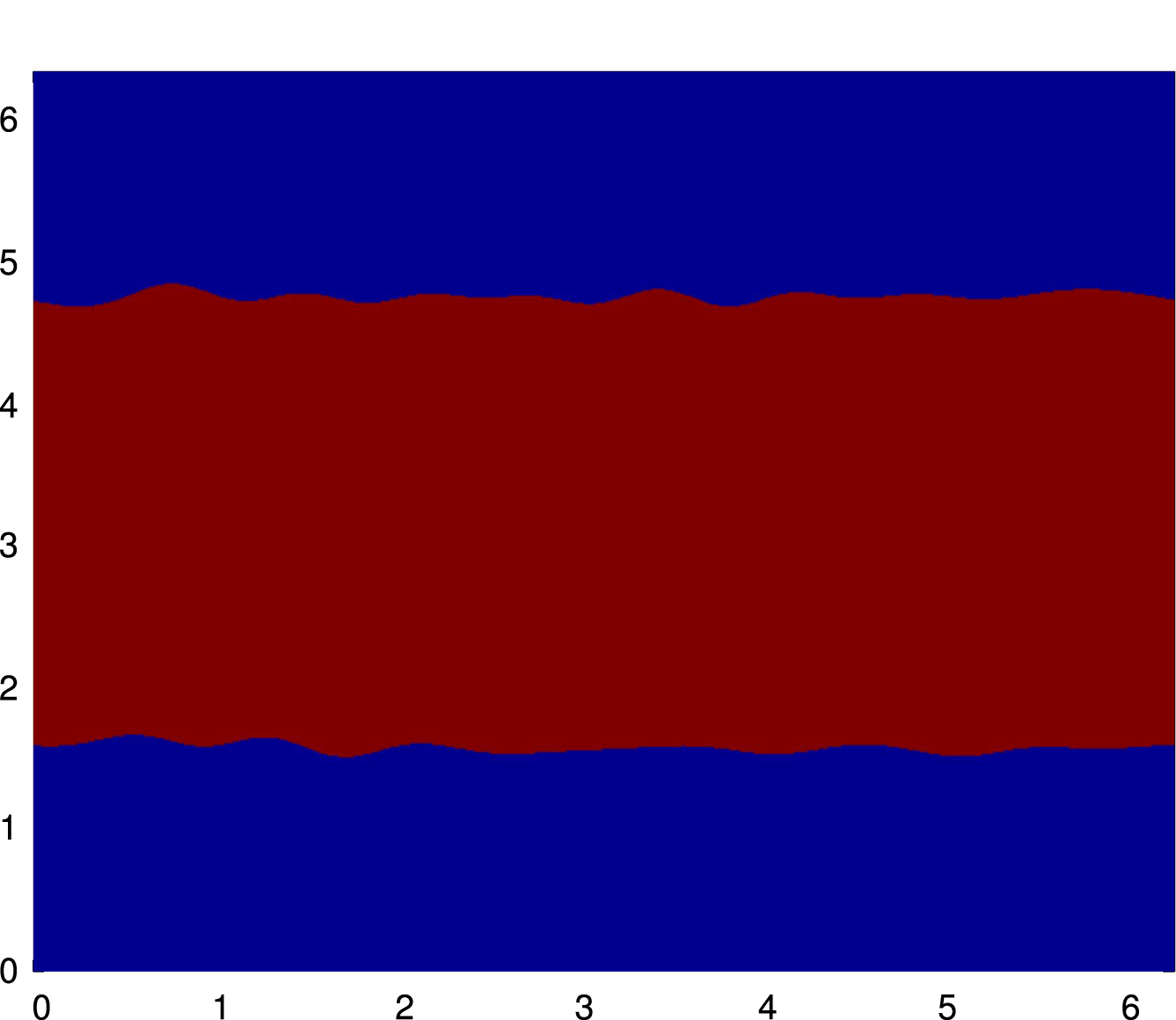
Passively advected tracer at  $t=2$ for
 ${\it\varepsilon}=0.0512$ (a), 0.0256 (b), 0.0128 (c), 0.0064 (d).
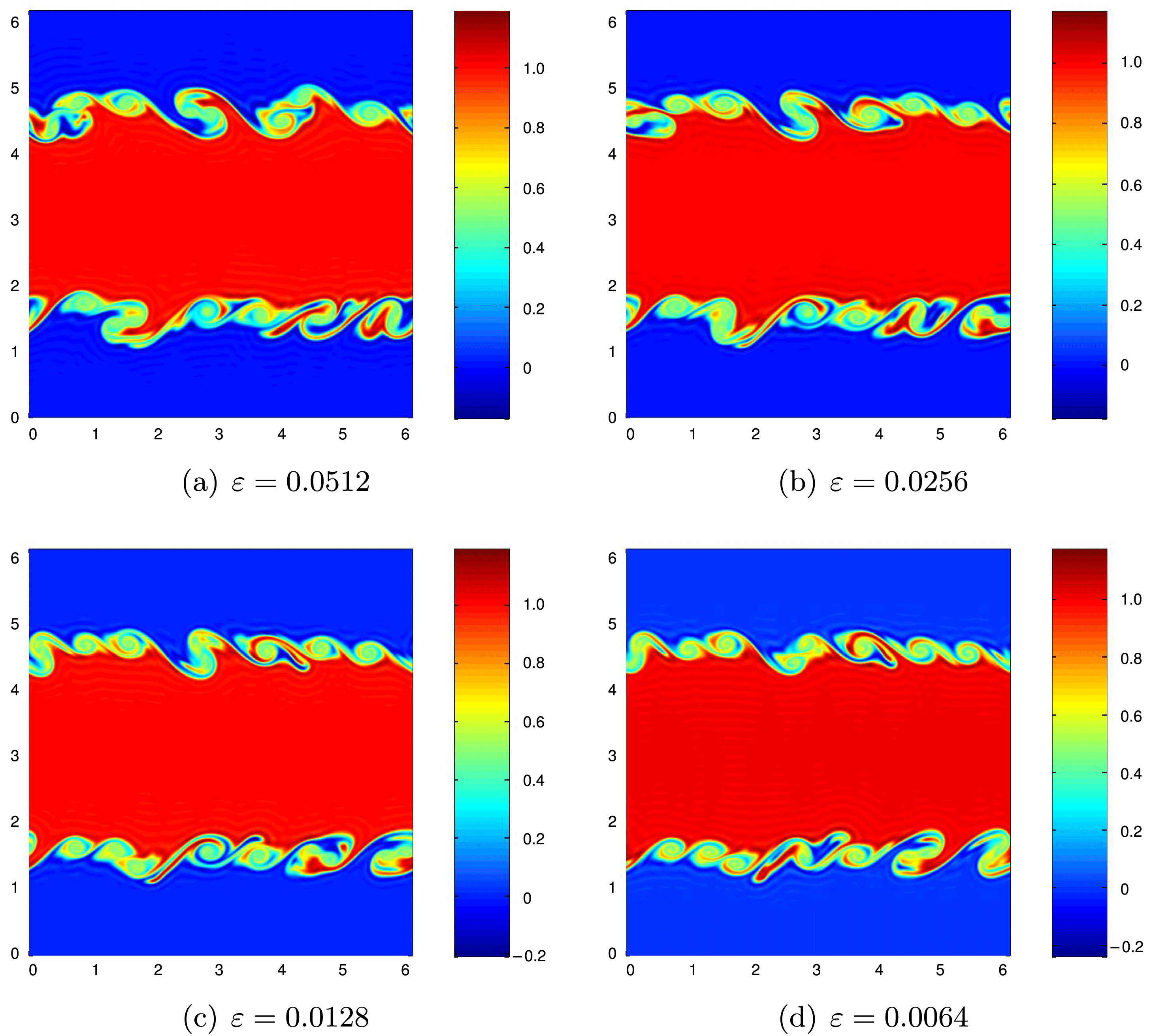
Cauchy rates ( $L^{2}$ differences in successive approximations) with respect to
 ${\it\varepsilon}$ for a single sample of the flat vortex sheet (8.1).
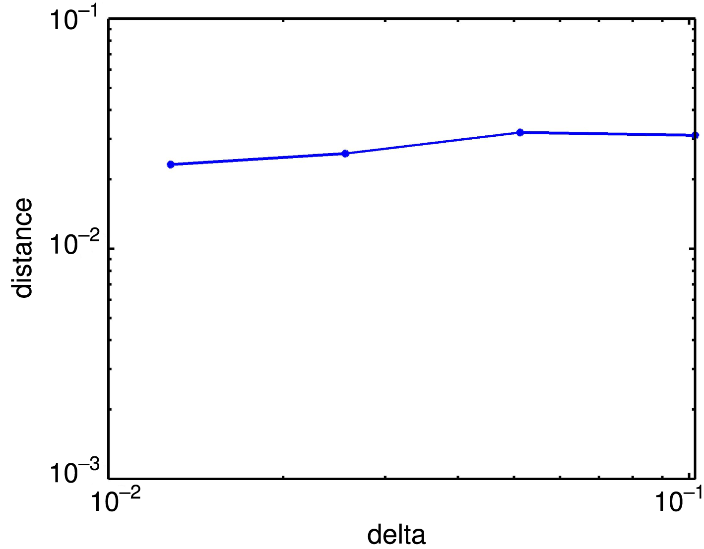
We further introduce perturbations of the two interfaces by making a perturbation ansatz for each interface of the form
 $$\begin{eqnarray}I({\it\omega};x)={\it\varepsilon}\mathop{\sum }_{k=1}^{K}{\it\alpha}_{k}({\it\omega})\sin (kx_{1}-{\it\beta}_{k}({\it\omega}))\end{eqnarray}$$
for uniformly distributed random numbers  ${\it\alpha}_{1},\ldots ,{\it\alpha}_{K}\in \mathbb{R}$,
 ${\it\beta}_{1},\ldots ,{\it\beta}_{K}\in [0,2{\it\pi})$ with
 $\sum _{k=1}^{K}|{\it\alpha}_{k}|^{2}=1$. The parameters
 $\{{\it\alpha}_{k},{\it\beta}_{k}\}_{1\leq k\leq K}$ are independent random variables that are different for the two interfaces. For our computations, we used a fixed value of
 $K=10$ perturbation modes.
The result of this ansatz is a random field
 $$\begin{eqnarray}u_{0}^{{\it\rho}}(x_{1},x_{2}-I(x,{\it\omega}))\end{eqnarray}$$
depending on two parameters  ${\it\rho}$ and
 ${\it\varepsilon}$. The parameter
 ${\it\varepsilon}$ controls the magnitude of the perturbation, while
 ${\it\rho}$ determines the smoothness across the interfaces. Projecting this random field back to the space of divergence-free vector fields using the Leray projection, we obtain our perturbed initial data
 $u_{0}^{{\it\rho},{\it\varepsilon}}$, as illustrated in Figure 8.1. For a fixed number of Fourier modes
 $N$, we aim to compute the corresponding approximate Young measure
 ${\it\nu}^{{\it\rho},{\it\varepsilon},N}$ using the spectral method from Section 6.1.1 in Step 2 of Algorithm 4.3). The measure-valued solution of (1.3) will then be realized as a limit of
 ${\it\nu}^{{\it\rho},{\it\varepsilon},N}$ as
 $N\rightarrow \infty$ and
 ${\it\rho},{\it\varepsilon}\rightarrow 0$.
8.1.1 Single realization
First, we fix a single realization of the random field  $u_{0}({\it\omega})$. To visualize the resulting approximate solutions, we plot the local kinetic energy at time
 $t=2$ in Figure 1.5. The results for this figure were obtained using
 ${\it\varepsilon}=0.01$,
 ${\it\rho}=0.001$ and different Fourier modes
 $N$. We see from the figure that as the resolution is increased, the distribution of kinetic energy is quite different for each resolution. In particular, the energy seems to concentrate on structures at ever smaller scales. This indicates that the underlying velocity field may not converge as the number of Fourier modes is increased. This is indeed verified in Figure 1.6, where we show the successive
 $L^{2}$ differences of the approximate velocity field (1.4) . The differences do not seem to go to zero, indicating that the approximate solutions may not form a Cauchy sequence, let alone converge.
Next, we consider the stability with respect to the perturbation parameter  ${\it\varepsilon}$ of single realizations of approximate solutions. We fix
 $N=512$ and compute for different values of
 ${\it\varepsilon}$. To visualize the resulting solution, we plot a tracer, initially concentrated in
 $x_{2}\in [{\it\pi}/2,3{\it\pi}/2]$ and passively advected by the computed velocity field. We show the passively advected tracer at time
 $t=2$ in Figure 8.2. The figure clearly shows that the tracer distribution is very different for different values of
 ${\it\varepsilon}$. As shown in Figure 8.3, the
 $L^{2}$ difference for successive values of
 ${\it\varepsilon}$ does not decrease as
 ${\it\varepsilon}$ decreases. Hence, the perturbed solutions do not converge as the perturbation tends to zero, indicating instability of the flat vortex sheet (8.1) with respect to perturbations.
Convergence of mean of the  $x$-component of the velocity at time
 $t=2$, for the flat vortex sheet with respect to
 $N$ (number of Fourier modes).
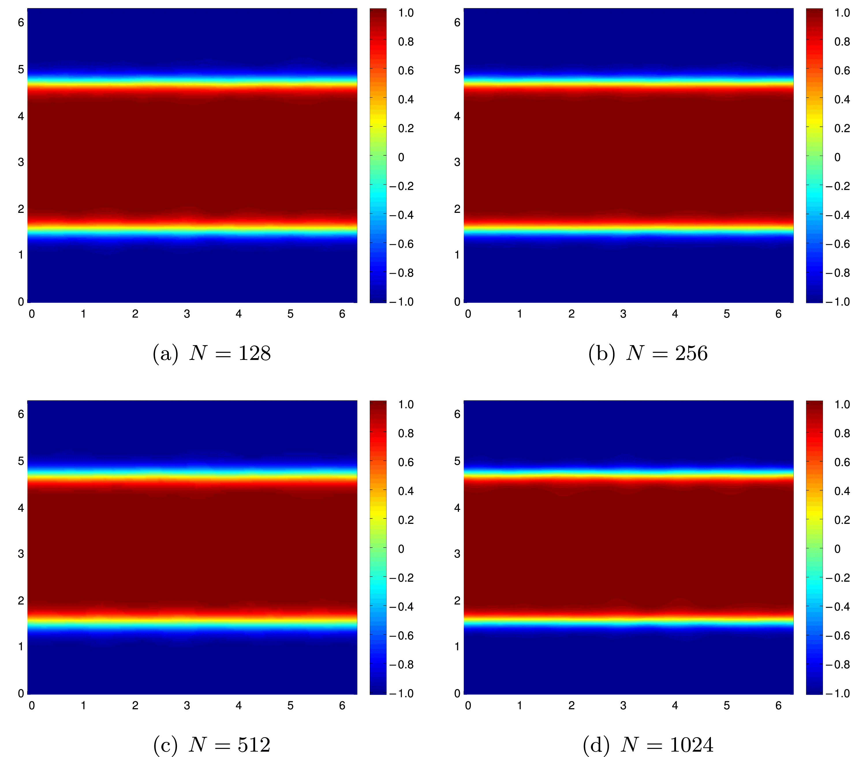
8.1.2 Ensemble of solutions
Having seen the lack of convergence and stability for single realizations of the perturbed vortex sheet, we apply Algorithm 4.3 to compute the approximate Young measure. To this end, we use the Monte Carlo Algorithm 4.4 with  $M=400$ samples. We compute the mean of the approximate measure-valued solution
 $$\begin{eqnarray}\langle {\it\nu}_{x,t}^{{\it\rho},{\it\varepsilon},N,M},\,{\it\xi}\rangle =\frac{1}{M}\mathop{\sum }_{i=1}^{M}v^{{\it\rho},{\it\varepsilon},N,i}(x,t)\end{eqnarray}$$
as well as the second moments
 $$\begin{eqnarray}\langle {\it\nu}_{x,t}^{{\it\rho},{\it\varepsilon},N,M},\,{\it\xi}\otimes {\it\xi}\rangle =\frac{1}{M}\mathop{\sum }_{i=1}^{M}(v^{{\it\rho},{\it\varepsilon},N,i}\otimes v^{{\it\rho},{\it\varepsilon},N,i})(x,t).\end{eqnarray}$$
The mean of  $u_{1}$ and the second component of
 $u_{2}$ at time
 $t=2$, computed for different number of Fourier modes, are shown in Figures 8.4 and 8.5. In complete contrast to Figure 1.5 (which uses a single sample), and as predicted by Theorem 6.4, both the mean and the variance seem to converge as the number of Fourier modes is increased. This convergence is further verified in Figure 8.6, which displays successive
 $L^{2}$ differences of the mean velocity field and the second moment
 ${\it\xi}_{2}{\it\xi}_{2}$. The convergence in the second moment is slower than that of the mean; this is not unexpected as we use the same samples for the computation of the mean and the second moment. Furthermore, from Figures 8.4 and 8.5 we observe that small-scale features are averaged out in the statistical quantities such as the mean and variance.
Convergence of second moment of the  $y$-component of the velocity at time
 $t=2$, for the flat vortex sheet, with respect to
 $N$ (number of Fourier modes).
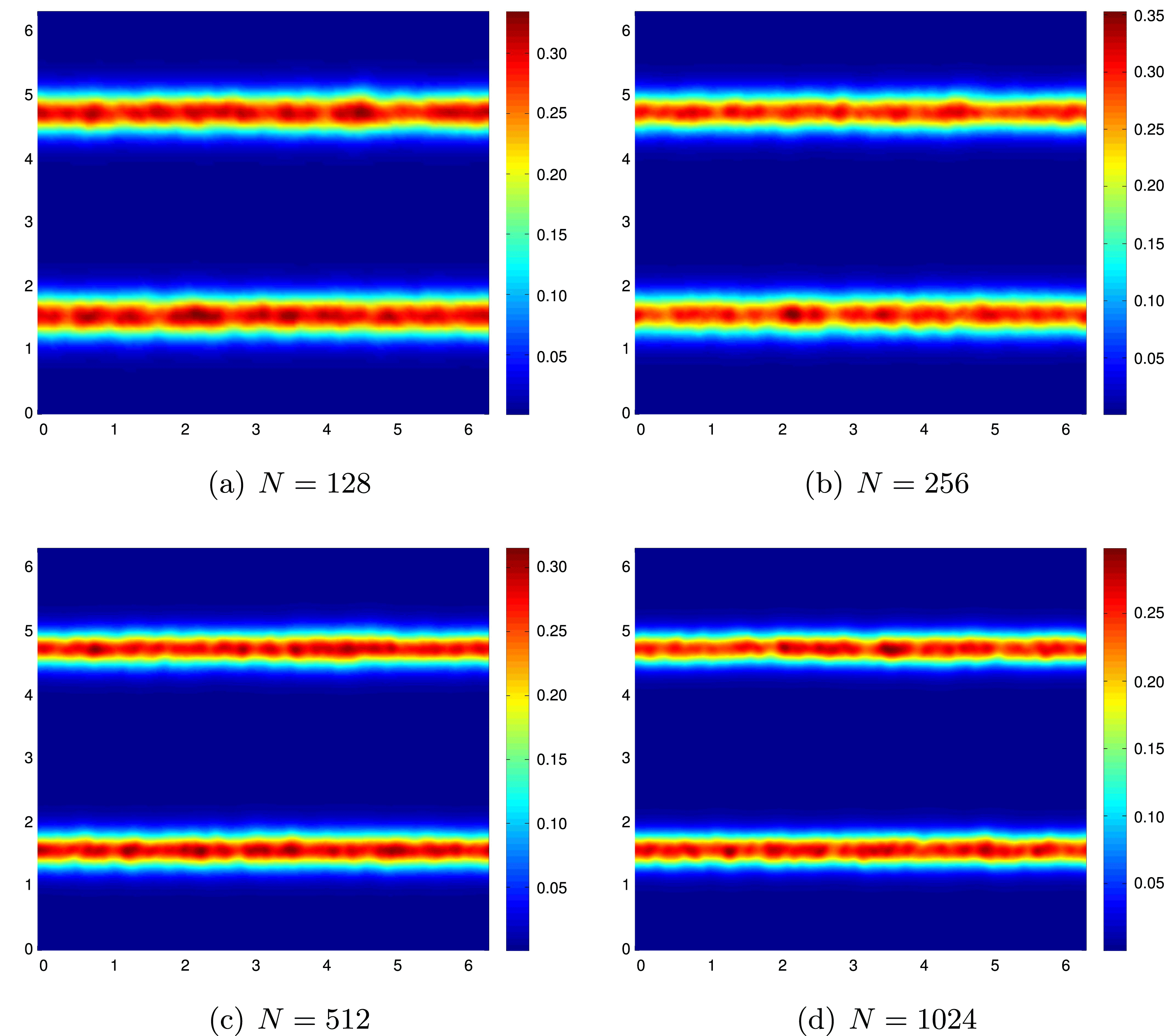
Cauchy rates with respect to  $N$, at time
 $t=2$.
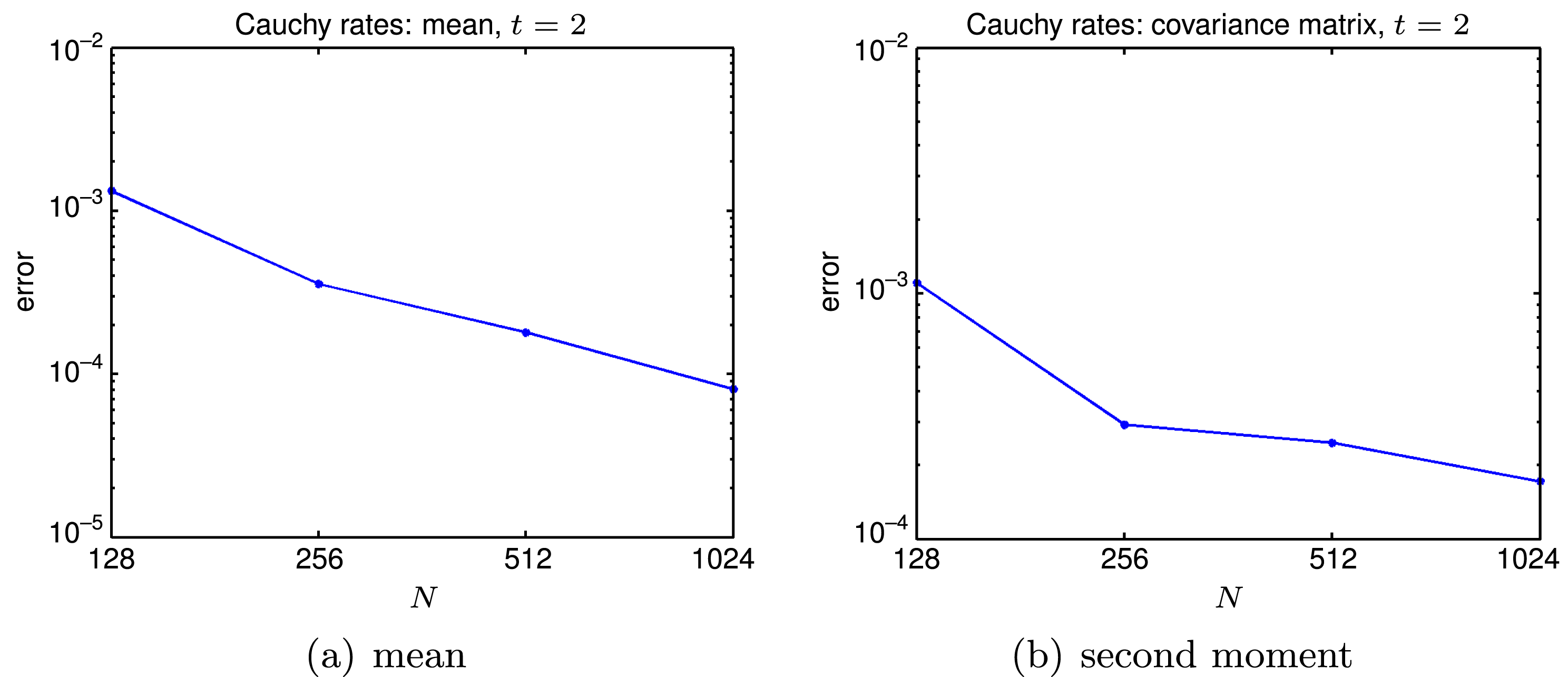
As we are approximating atomic initial Young measure concentrated on the flat vortex sheet (8.1) by the perturbation-based Algorithm 4.3, we will let the perturbation parameter  ${\it\varepsilon}\rightarrow 0$. For this purpose, we fix
 $N=512$ and consider approximate Young measures
 ${\it\nu}^{{\it\rho},{\it\varepsilon},N}$ for successively smaller values of
 ${\it\varepsilon}$. The results for the mean of the first component of the velocity field and the variance of the second component of the velocity field are plotted in Figures 8.7 and 8.8. The figures indicate that these statistical quantities also converge with decreasing perturbation amplitude. This convergence is verified in Figure 8.9, where successive
 $L^{2}$ differences of the mean and the second moment are displayed.
Convergence of mean, at time  $t=2$, for the
 $x$-component of the velocity, with respect to
 ${\it\varepsilon}$.
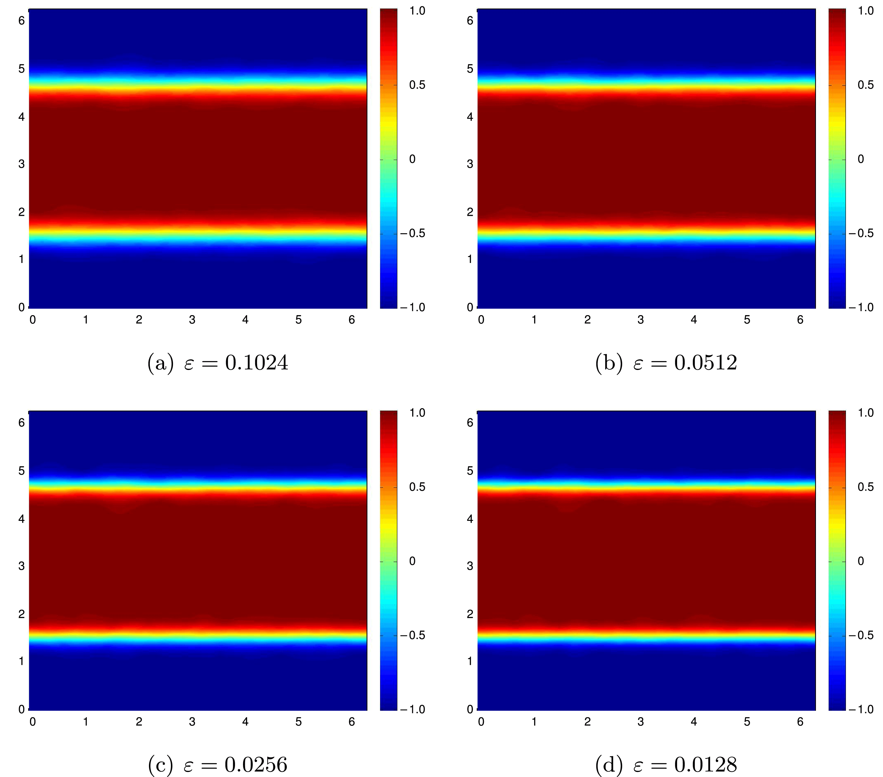
Convergence of second moment at time  $t=2$, for the
 $y$-component of the velocity field, with respect to
 ${\it\varepsilon}$.
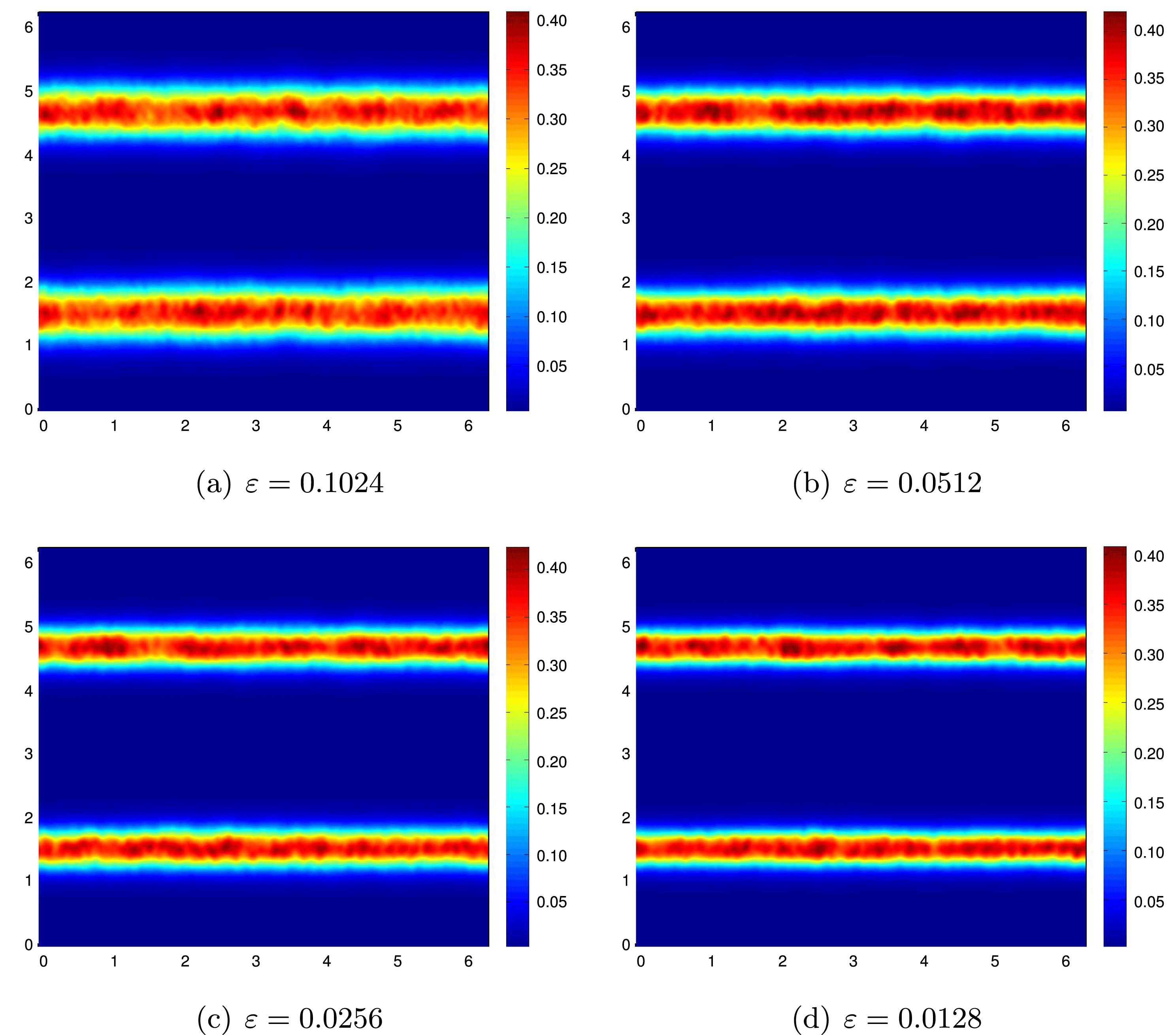
Cauchy rates with respect to  ${\it\varepsilon}$.
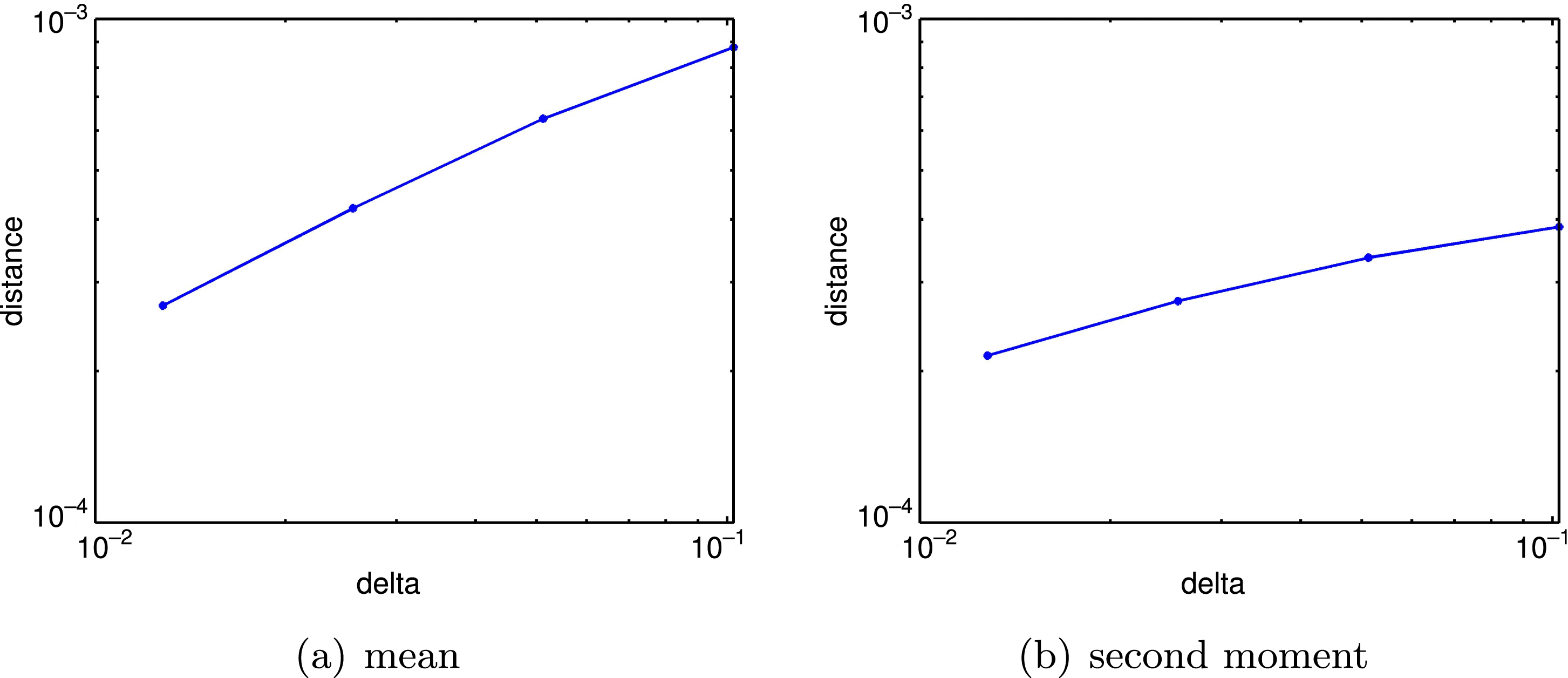
The convergence results for statistical quantities such as the mean and the variance, with respect to the resolution and the perturbation parameter, are consistent with the prediction of weak* convergence in Theorem 6.4. The convergence in fact seems to be even stronger than the predicted weak* convergence. To test this assertion, the 1-Wasserstein distance between successive approximations  ${\it\varepsilon}$ and
 ${\it\varepsilon}/2$ was computed and presented in Figure 14 of Lanthaler and Mishra (Reference Lanthaler and Mishra2015). This figure demonstrated convergence in the stronger 1-Wasserstein metric as
 ${\it\varepsilon}\rightarrow 0$.
As the initial data are an atomic measure in this case, it is interesting to find out whether the computed admissible measure-valued solution is also atomic. To this end, we make use of a symmetry property of the limit Young measure (Theorem 5.1(2) of Lanthaler and Mishra Reference Lanthaler and Mishra2015) that it would be invariant in the  $x_{1}$-direction. We fix
 $N=512$, and present an
 $x_{1}=\text{const.}$ slice of the mean and the variance of the velocity field
 $v_{1}$ in the
 $x_{2}$-direction for different values of
 ${\it\varepsilon}$. The results shown in Figure 8.10 show that there is convergence as
 ${\it\varepsilon}\rightarrow 0$. Furthermore, the mean in the
 ${\it\varepsilon}\rightarrow 0$ limit does not coincide with the initial velocity profile. The variance is also very different from zero, with two distinct non-zero patches (which are symmetric with respect to
 $x_{2}={\it\pi}$). We call these two patches the turbulence zones. These results strongly indicate that the computed measure-valued solution is not atomic. We remark that this non-atomicity of the limit Young measure is presented in Lanthaler and Mishra (Reference Lanthaler and Mishra2015) as convincing numerical evidence for the non-uniqueness of Delort solutions of the incompressible Euler equations.
One-dimensional slices of the mean (a) and the variance (b) computed with different values of  ${\it\varepsilon}$.
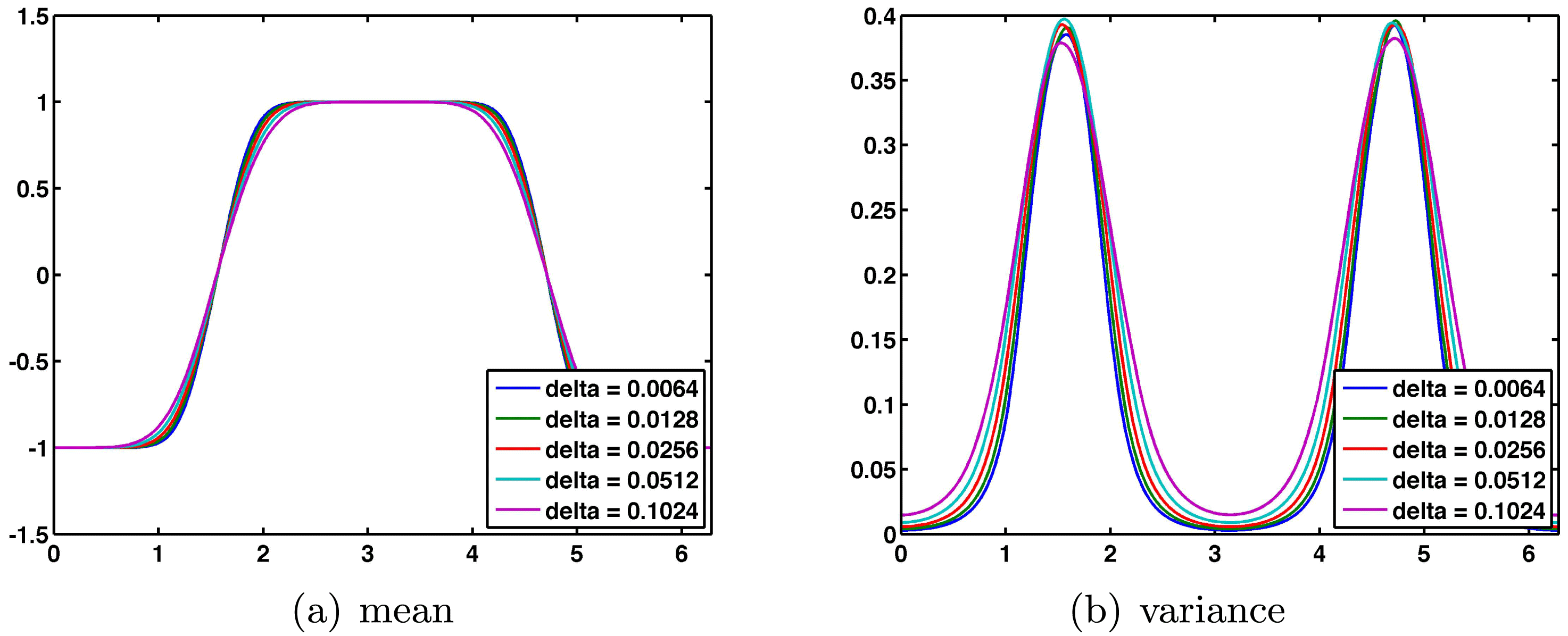
8.2 Stability/uniqueness of computed measure-valued solutions
Next, we examine whether the computed measure-valued solutions are stable in a suitable sense. Following Fjordholm et al. (Reference Fjordholm, Käppeli, Mishra and Tadmor2016a) and Lanthaler and Mishra (Reference Lanthaler and Mishra2015), we observe that Algorithm 4.3 (and Algorithm 4.4) rely on two inputs, the numerical method (in Step 2 of Algorithm 4.3) and the type of perturbations (modelled by the random field  $X$ in Step 1 of Algorithm 4.3). Both these inputs can be chosen freely provided that they satisfy some structural properties, for instance those required of the numerical method in Theorem 5.1. We wish to investigate whether the computed measure-valued solutions – at least for atomic initial data – are stable with respect to the choice of numerical method and to the choice of random initial perturbations. This issue is investigated in Fjordholm et al. (Reference Fjordholm, Käppeli, Mishra and Tadmor2016a) in the context of compressible Euler equations and in Lanthaler and Mishra (Reference Lanthaler and Mishra2015) for the incompressible Euler equations. We present some results for the incompressible Euler equations from Lanthaler and Mishra (Reference Lanthaler and Mishra2015) below.
8.2.1 Stability with respect to the numerical method
We have described two very different numerical methods for approximating the incompressible Euler equations (1.3): the spectral (viscosity) method (6.4) and the finite difference projection method (6.7). Both were shown to converge to a measure-valued solution of the incompressible Euler equations, but do they converge to the same measure-valued solution? To answer this question, we use Algorithm 4.3 to compute measure-valued solutions for the flat vortex sheet (8.1). We fix the same initial random field as described in Section 8.1 with parameters  $({\it\rho},{\it\varepsilon})=(0.001,0.01)$, and compute the resulting measure-valued with the spectral method (6.4) and the finite difference projection method (6.7) with
 $512$ Fourier modes and
 $512$ mesh points (in each direction), respectively. The mean and variance of the computed measure-valued solution for the spectral method (6.4) has already been shown in Figures 8.4 and 8.5(d), respectively. The mean and variance of the measure-valued solution, computed with the finite difference projection method (6.7), is shown in Figure 8.11. A comparison of the two sets of figures clearly shows that the statistics of the measure-valued solution, computed with two very different methods, are very similar. Hence, and also based on a similar comparison between different methods for approximating the compressible Euler equations, it appears that the computed measure-valued solution is very stable with respect to the choice of numerical methods.
Flat vortex sheet: (a) mean of the  $x$-component of the velocity field, (b) second moment of
 $y$-component of the velocity field (from Leonardi and Mishra Reference Leonardi and Mishra2016) on a
 $512^{2}$ grid, to be compared with the spectral method.
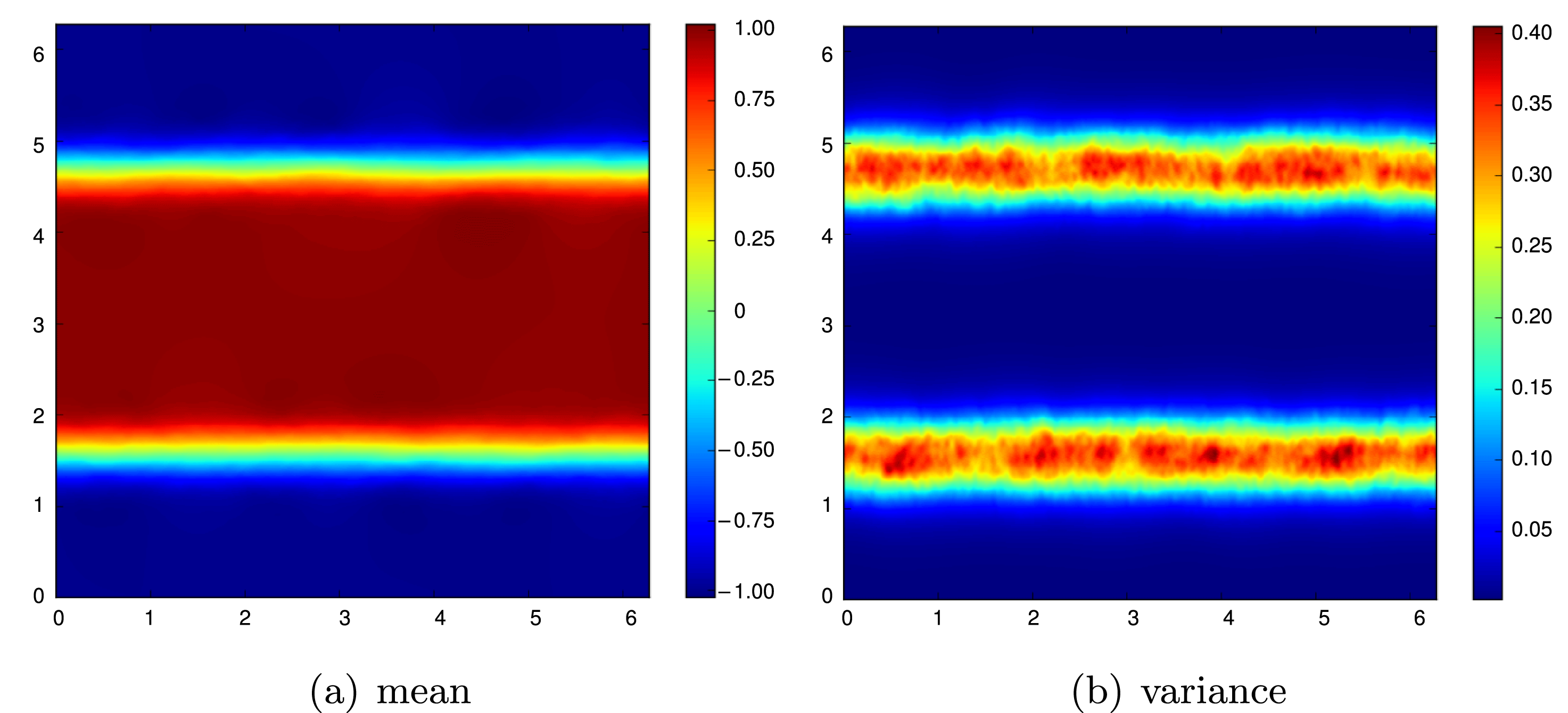
8.2.2 Stability with respect to different perturbations
Having demonstrated the robustness of Algorithm 4.3 with respect to the choice of numerical method in Step 2, we investigate whether the algorithm is sensitive with respect to the type of perturbations in Step 1. To do this, we consider the most general perturbation to the initial data (8.1) by adding a random field that is constant on local patches, and which exhibits uncorrelated fluctuations of equal strength in all of space. More precisely, we consider random fields of the form  $X^{0}=\sum _{i,j}X_{i,j}^{0}1_{{\mathcal{C}}_{i,j}}$, where the patches are
 $$\begin{eqnarray}{\mathcal{C}}_{i,j}=\{(x,y)\in \mathbb{T}^{2}:\text{i}k{\rm\Delta}x\leq x<(i+1)k{\rm\Delta}x,\,jk{\rm\Delta}y\leq y<(j+1)k{\rm\Delta}y\},\end{eqnarray}$$
with  $k=16$ comprising
 $16\times 16$ mesh cells. The random variables
 $X_{i,j}^{0}$ are independent and identically distributed random variables, uniformly distributed, with respect to the Lebesgue measure, on
 $[-1,1]^{2}$. We obtain our initial perturbations
 $Z_{{\it\delta}}^{0}$ as the projection of
 $u_{0}+{\it\delta}X^{0}$ to the space of divergence-free vector fields. We refer to the results obtained from this perturbation procedure as ‘uncorrelated’ below.
Note that we can (formally) rewrite the evolution equation for the mean  $\overline{{\it\nu}}$ of the measure-valued solutions of incompressible Euler equations (1.3) as
 $$\begin{eqnarray}\partial _{t}\overline{{\it\nu}}+\overline{{\it\nu}}\cdot {\rm\nabla}\overline{{\it\nu}}+{\rm\nabla}p=-\text{div}\langle {\it\nu},({\it\xi}-\overline{{\it\nu}})\otimes ({\it\xi}-\overline{{\it\nu}})\rangle .\end{eqnarray}$$
If the fluctuations of the mean  $\overline{{\it\nu}}$ in the neighbourhood of any given point are an indication of the fluctuations of
 ${\it\nu}$, then we should expect the relevant contributions to the evolution of
 $\overline{{\it\nu}}$ to originate at the two interfaces, where
 $\overline{{\it\nu}}$ has a large jump. Hence, we localize the above uncorrelated perturbation to the initial data by multiplying it with cut-off functions that are supported around the two interfaces. We refer to the results from these localizations as ‘uniform’ or ‘Gaussian’ according to the corresponding distribution the values of the
 $X_{i,j}^{0}$ were chosen from. Hence, ‘uniform’ and ‘Gaussian’ refer to the localized perturbations around the interfaces, but with uniformly and normally distributed random variables, respectively. The results of applying Algorithm 4.3 with these perturbations, with amplitude
 ${\it\varepsilon}=0.05$ and the spectral method (6.4), are shown in Figures 8.12 (mean) and 8.13 (second moment) at time
 $t=4$. Clearly the computed solutions are very similar to those computed with the sinusoidal perturbations, described in Section 8.1. Thus, the nature of underlying distribution does not seem to affect the computed measure-valued solution.
Flat vortex sheet: mean for the  $x$-component of the velocity field, at time
 $t=2$, computed with
 $N=1024$ Fourier modes and with different types of initial perturbations.
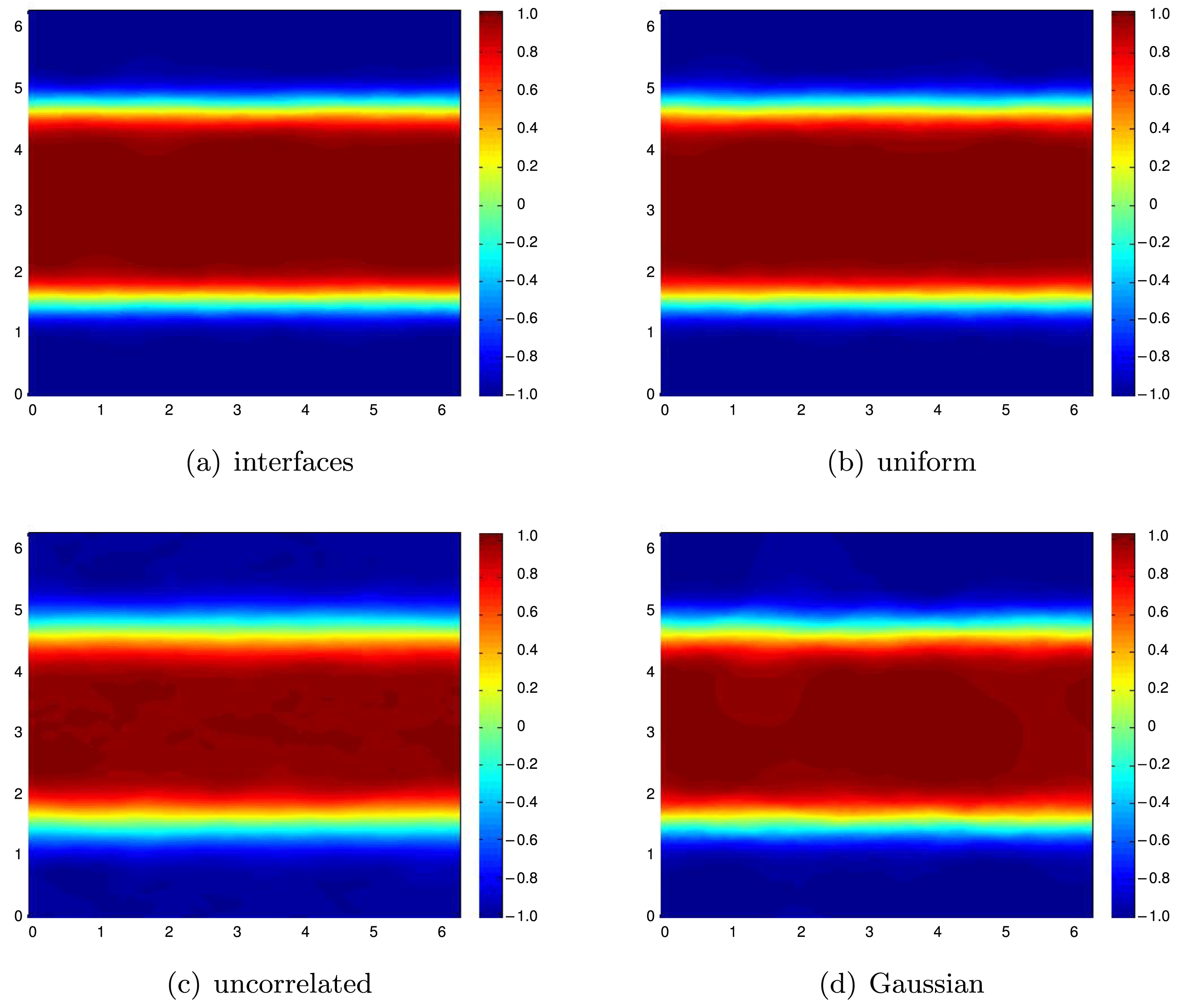
Flat vortex sheet: second moment for the  $y$-component of the velocity field, at time
 $t=2$, computed with
 $N=1024$ Fourier modes and with different types of perturbations.
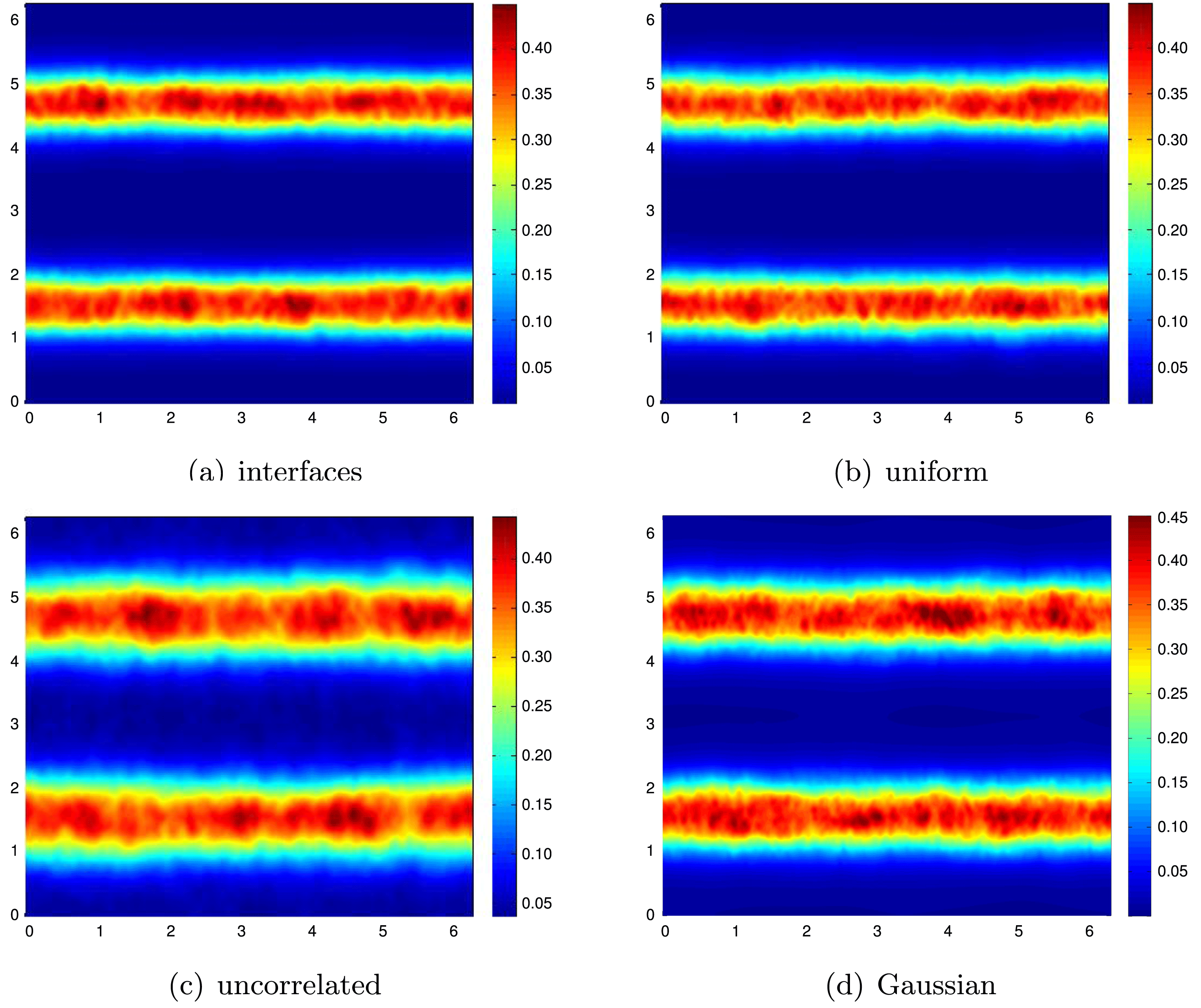
Summarizing these results and those for the compressible Euler equations presented in Fjordholm et al. (Reference Fjordholm, Käppeli, Mishra and Tadmor2016a), we see that the computed measure-valued solutions are stable with respect to the type of initial perturbations as well as to the underlying numerical method that approximates them, at least when the initial data are atomic.
PART THREE
Related concepts, methods and applications
9 Statistical solutions
The numerical experiments in Sections 7 and 8 strongly hint that measure-valued solutions behave in a much more stable, predictable manner than do individual (approximate) weak solutions. However, it is fairly easy to see that non-atomic measure-valued solutions are non-unique. We include here a counter-example to uniqueness, taken from Fjordholm et al. (Reference Fjordholm, Käppeli, Mishra and Tadmor2016a).
Example 9.1. Consider the Burgers equation,
 $$\begin{eqnarray}\partial _{t}u+\partial _{x}\biggl(\frac{u^{2}}{2}\biggr)=0.\end{eqnarray}$$
Let  ${\it\lambda}$ denote the Lebesgue measure on
 $\mathbb{R}$ and let
 ${\it\lambda}_{A}$ be the restriction of
 ${\it\lambda}$ to a subset
 $A\subset \mathbb{R}$, that is,
 ${\it\lambda}_{A}(B)={\it\lambda}(A\cap B)$. We define
 ${\rm\Omega}=[0,1]$,
 ${\mathcal{X}}={\mathcal{B}}([0,1])$ (the Borel
 ${\it\sigma}$-algebra on
 $[0,1]$) and
 $P={\it\lambda}_{[0,1]}$. Let
 $u_{0}$ and
 $\widetilde{u}_{0}$ be the random fields
 $$\begin{eqnarray}\displaystyle u_{0}({\it\omega};x):=\left\{\begin{array}{@{}ll@{}}1+{\it\omega}\quad & \text{for }x<0,\\ {\it\omega}\quad & \text{for }x>0,\end{array}\right.\quad \widetilde{u}_{0}({\it\omega};x):=\left\{\begin{array}{@{}ll@{}}1+{\it\omega}\quad & \text{for }x<0,\\ 1-{\it\omega}\quad & \text{for }x>0,\end{array}\right. & & \displaystyle \nonumber\end{eqnarray}$$
for  ${\it\omega}\in [0,1],~x\in \mathbb{R}$. It is readily checked that the law of both
 $u_{0}$ and
 $\widetilde{u}_{0}$ in
 $({\rm\Omega},{\mathcal{X}},P)$ equals
 $$\begin{eqnarray}{\it\sigma}_{x}=\left\{\begin{array}{@{}ll@{}}{\it\lambda}_{[1,2]}\quad & \text{for }x<0,\\ {\it\lambda}_{[0,1]}\quad & \text{for }x>0.\end{array}\right.\end{eqnarray}$$
The entropy solutions  $u({\it\omega})$ and
 $\widetilde{u}({\it\omega})$ of the Riemann problems with initial data
 $u_{0}({\it\omega})$ and
 $\widetilde{u}_{0}({\it\omega})$ are given by
 $$\begin{eqnarray}u({\it\omega};x,t)=\left\{\begin{array}{@{}ll@{}}1+{\it\omega}\quad & \text{if }x/t<1/2+{\it\omega},\\ {\it\omega}\quad & \text{if }x/t>1/2+{\it\omega},\end{array}\right.\quad \widetilde{u}({\it\omega};x,t)=\left\{\begin{array}{@{}ll@{}}1+{\it\omega}\quad & \text{if }x/t<1,\\ 1-{\it\omega}\quad & \text{if }x/t>1,\end{array}\right.\end{eqnarray}$$
and it is straightforward to compute the pointwise laws  ${\it\nu}_{x,t}=\text{Law}(u(\cdot ;x,t))$ and
 $\widetilde{{\it\nu}}_{x,t}=\text{Law}(\widetilde{u}(\cdot ;x,t))$:
 $$\begin{eqnarray}\displaystyle {\it\nu}_{x,t} & = & \displaystyle \left\{\begin{array}{@{}ll@{}}{\it\lambda}_{[1,2]}\quad & \text{if }x/t<1/2,\\ {\it\lambda}_{[x/t+1/2,2]}+{\it\lambda}_{[0,x/t-1/2]}\quad & \text{if }1/2<x/t<3/2,\\ {\it\lambda}_{[0,1]}\quad & \text{if }3/2<x/t,\end{array}\right.\nonumber\\ \displaystyle \widetilde{{\it\nu}}_{x,t} & = & \displaystyle \left\{\begin{array}{@{}ll@{}}{\it\lambda}_{[1,2]}\quad & \text{if }x/t<1,\\ {\it\lambda}_{[0,1]}\quad & \text{if }x/t>1.\end{array}\right.\nonumber\end{eqnarray}$$
Both  ${\it\nu}_{x,t}$ and
 $\widetilde{{\it\nu}}_{x,t}$ converge to
 ${\it\sigma}_{x}$strongly as
 $t\rightarrow 0$ for all
 $x\neq 0$. Thus,
 ${\it\nu}$ and
 $\widetilde{{\it\nu}}$ are EMV solutions with the same initial MV data
 ${\it\sigma}$, but do not coincide.
For more counter-examples, see Schochet (Reference Schochet1989). It is clear that as soon as the measure  ${\it\nu}_{x,t}$ spreads out (i.e., it becomes non-atomic, which in Example 9.1 happens at
 $t=0$), one can parametrize
 ${\it\nu}_{x,t}$ as distinct random fields
 $u({\it\omega};x,t)$ and
 $\widetilde{u}({\it\omega};x,t)$, leading to distinct measure-valued solutions
 ${\it\nu}_{x,s}$ and
 $\widetilde{{\it\nu}}_{x,s}$ for
 $s>t$. This deficiency is inherent to measure-valued solutions and it seems unlikely that any type of entropy condition can avoid it.
9.1 Solutions as random fields
The first remedy that might come to mind is to define a ‘solution’ to be precisely a random field  $u({\it\omega};x,t)$ which satisfies the PDE in some strong (e.g.,
 $u({\it\omega})$ is an entropy solution for all
 ${\it\omega}\in {\rm\Omega}$) or weak sense (e.g., the PDE holds when integrated against some class of test functions
 ${\rm\Phi}({\it\omega})$). The former is an approach taken in several works on stochastic conservation laws; see, for example, Mishra and Schwab (Reference Mishra and Schwab2012) and references therein, as well as Section 10. The parameter
 ${\it\omega}$ is usually a point in some abstract probability space
 $({\rm\Omega},{\mathcal{X}},P)$. But it is always possible to reparametrize the random field
 $u({\it\omega})$ as
 $\widetilde{u}(\widetilde{{\it\omega}})$ over a different space
 $(\widetilde{{\rm\Omega}},\widetilde{{\mathcal{X}}},\widetilde{P})$, yielding a distinct ‘solution’ (albeit with the same statistical properties). Hence, the approach of random field solutions is inherently non-unique.
9.2 Statistical solutions I
A refinement of the random field approach which is independent of arbitrary parametrizations is to consider only the law of the above random fields. If, for example,  $u({\it\omega};\cdot ,t)\in L^{p}(D)$ for all
 ${\it\omega}\in {\rm\Omega}$ and
 $t\geq 0$, then the law of
 $u$ would be a probability measure on
 $L^{p}(D)$:
 $$\begin{eqnarray}{\it\mu}_{t}=\text{Law}({\it\omega}\mapsto u({\it\omega};\cdot ,t))\in {\mathcal{P}}(L^{p}(D)).\end{eqnarray}$$
Pointwise reparametrizations such as in Example 9.1 would no longer be possible, since such a reparametrization would inevitably give rise to distinct laws  ${\it\mu}_{t}$,
 $\widetilde{{\it\mu}}^{t}$ (although possibly with the same pointwise laws). The idea of a (time-parametrized) probability measure as the solution of a PDE was introduced by Foiaş (Reference Foiaş1972, Reference Foiaş1973) (see also Foiaş, Manley, Rosa and Temam Reference Foiaş, Manley, Rosa and Temam2001), who defined statistical solutions of the Navier–Stokes equations. A statistical solution of a PDE (e.g., the Navier–Stokes equations) is a time-parametrized map
 $t\mapsto {\it\mu}_{t}\in {\mathcal{P}}({\mathcal{F}})$ for some appropriate function space
 ${\mathcal{F}}$, which satisfies the PDE in some weak sense. A major challenge in this context is to find the appropriate weak formulation of the PDE: it must be strong enough to yield uniqueness of solutions, but not so strong that it depends on the existence of a solution operator
 $u_{0}\mapsto u(t)$; as the numerical experiments in Sections 7 and 8 suggest, there may not exist a well-defined solution operator within
 ${\mathcal{F}}=L^{p}(D)$, for any
 $1\leq p\leq \infty$.
9.3 Correlation measures
An alternative approach to avoiding the kind of deficiencies seen in Example 9.1 is to add information about correlations. In this example we were free to parametrize  ${\it\nu}_{x_{1}}$ however we wanted, independent of the parametrization of
 ${\it\nu}_{x_{2}}$ at any other point
 $x_{2}$. To counteract this, we can add information about two-point correlation in the form of a Young measure
 ${\it\nu}_{x_{1},x_{2}}^{2}$ for every pair
 $(x_{1},x_{2})\in D^{2}$. The number
 ${\it\nu}_{x_{1},x_{2}}^{2}(A_{1}\times A_{2})$ can be interpreted as ‘the probability that
 $u(x_{1})\in A_{1}$and
 $u(x_{2})\in A_{2}$’; compare this with the interpretation of
 ${\it\nu}_{x_{1}}(A_{1})$ as ‘the probability that
 $u(x_{1})\in A_{1}$’. The two-point correlations of the two initial random fields in Example 9.1 are
 $$\begin{eqnarray}\displaystyle {\it\sigma}_{x_{1},x_{2}}^{2}({\it\xi}_{1},{\it\xi}_{2}) & = & \displaystyle \left\{\begin{array}{@{}ll@{}}{\it\delta}_{{\it\xi}_{1}}({\it\xi}_{2}){\it\lambda}_{[1,2]}({\it\xi}_{1})\quad & \text{if }x_{1},x_{2}<0,\\ {\it\delta}_{{\it\xi}_{1}+1}({\it\xi}_{2}){\it\lambda}_{[0,1]}({\it\xi}_{1})\quad & \text{if }x_{1}<0<x_{2},\\ {\it\delta}_{{\it\xi}_{1}-1}({\it\xi}_{2}){\it\lambda}_{[1,2]}({\it\xi}_{1})\quad & \text{if }x_{2}<0<x_{1},\\ {\it\delta}_{{\it\xi}_{1}}({\it\xi}_{2}){\it\lambda}_{[0,1]}({\it\xi}_{1})\quad & \text{if }0<x_{1},x_{2},\end{array}\right.\nonumber\\ \displaystyle \widetilde{{\it\sigma}}_{x_{1},x_{2}}^{2}({\it\xi}_{1},{\it\xi}_{2}) & = & \displaystyle \left\{\begin{array}{@{}ll@{}}{\it\delta}_{{\it\xi}_{1}}({\it\xi}_{2}){\it\lambda}_{[1,2]}({\it\xi}_{1})\quad & \text{if }x_{1},x_{2}<0,\\ {\it\delta}_{2-{\it\xi}_{1}}({\it\xi}_{2}){\it\lambda}_{[0,1]}({\it\xi}_{1})\quad & \text{if }x_{1}<0<x_{2},\\ {\it\delta}_{2-{\it\xi}_{1}}({\it\xi}_{2}){\it\lambda}_{[1,2]}({\it\xi}_{1})\quad & \text{if }x_{2}<0<x_{1},\\ {\it\delta}_{{\it\xi}_{1}}({\it\xi}_{2}){\it\lambda}_{[0,1]}({\it\xi}_{1})\quad & \text{if }0<x_{1},x_{2}.\end{array}\right.\nonumber\end{eqnarray}$$
Since these are clearly distinct, the two-point correlations  ${\it\sigma}^{2}$,
 $\widetilde{{\it\sigma}}^{2}$ can ‘tell the difference’ between the two random fields, even though they have the same one-point statistics
 ${\it\sigma}$. A more sophisticated choice of random fields
 $u$,
 $\widetilde{u}$ could, however, have the same one- and two-point laws, but still parametrize different families of functions. This argument can be readily iterated to any number of points at which the statistical information is given. Thus, to address the shortcomings of measure-valued solutions pointed out in Example 9.1, one would have to consider a whole family
 ${\it\nu}^{1},{\it\nu}^{2},{\it\nu}^{3},\ldots \,$ of Young measures, the
 $k$th member of which would be a Young measure
 ${\it\nu}^{k}\in \mathbf{Y}(D^{k},(\mathbb{R}^{N})^{k})$, with the interpretation that
 ${\it\nu}_{x_{1},\ldots ,x_{k}}^{k}(A_{1}\times \cdots \times A_{k})$ is ‘the probability that
 $u(x_{i})\in A_{i}$ for all
 $i=1,\ldots ,k$’. The full definition is as follows. (Here and below we denote
 $U=\mathbb{R}^{N}$.)
Definition 9.2 (Fjordholm, Lanthaler and Mishra Reference Fjordholm, Lanthaler and Mishra2016b).
A correlation measure is a collection  ${\it\nu}=({\it\nu}^{1},{\it\nu}^{2},\ldots \,)$ satisfying the following properties.
(i) Weak* measurability. The map
${\it\nu}^{k}:D^{k}\rightarrow {\mathcal{P}}(U^{k})$ is weak*-measurable, in the sense that the map $x\mapsto \langle {\it\nu}_{x}^{k},\,f\rangle$ from $x\in D^{k}$ into $\mathbb{R}$ is Borel-measurable for all $f\in C_{0}(U^{k})$ and $k\in \mathbb{N}$. In other words, ${\it\nu}^{k}$ is a Young measure from $D^{k}$ to $U^{k}$.(ii)
$L^{p}$ boundedness. ${\it\nu}^{k}$ is bounded in ${\mathcal{F}}$, in the sense that (9.1)$$\begin{eqnarray}\Vert {\it\nu}^{k}\Vert _{p,k}:=\biggl(\int _{D^{k}}\langle {\it\nu}_{x}^{k},\,|{\it\xi}_{1}|^{p}\cdots |{\it\xi}_{k}|^{p}\rangle \text{d}x\biggr)^{1/p}\!\!<+\infty \quad \text{for all}~k\in \mathbb{N}.\end{eqnarray}$$(iii) Symmetry. If
${\it\sigma}$ is a permutation of $\{1,\ldots ,k\}$ and $f\in C_{0}(\mathbb{R}^{k})$, then for almost every$$\begin{eqnarray}\langle {\it\nu}_{{\it\sigma}(x)}^{k},\,f({\it\sigma}({\it\xi}))\rangle =\langle {\it\nu}_{x}^{k},\,f({\it\xi})\rangle\end{eqnarray}$$$x\in D^{k}$.(iv) Consistency. If
$f\in C_{0}(\mathbb{R}^{k})$ is of the form for some$$\begin{eqnarray}f({\it\xi}_{1},\ldots ,{\it\xi}_{k})=g({\it\xi}_{1},\ldots ,{\it\xi}_{k-1})\end{eqnarray}$$$g\in C_{0}(U^{k-1})$, then for almost every$$\begin{eqnarray}\langle {\it\nu}_{x_{1},\ldots ,x_{k}}^{k},\,f\rangle =\langle {\it\nu}_{x_{1},\ldots ,x_{k-1}}^{k-1},\,g\rangle\end{eqnarray}$$$(x_{1},\ldots ,x_{k})\in D^{k}$.










Each element  ${\it\nu}^{k}$ is called a correlation marginal. We let
 ${\mathcal{L}}^{p}={\mathcal{L}}^{p}(D,U)$ denote the set of all correlation measures from
 $D$ to
 $U$. We say that a correlation measure
 ${\it\nu}\in {\mathcal{L}}^{p}(D,U)$ is diagonally consistent (or DC) if, for all
 $k\in \mathbb{N}$, all
 $f\in C_{0}(U^{k+1})$ and almost every
 $x=(x_{1},\ldots ,x_{k})\in D^{k}$,
(i) the point
$(x_{1},\ldots ,x_{k},x_{k})\in D^{k+1}$ is a Lebesgue point for the map $D^{k+1}\ni y\mapsto \langle {\it\nu}_{y}^{k+1},\,f\rangle$, and(ii)
$\langle {\it\nu}_{x_{1},\ldots ,x_{k},x_{k}}^{k+1},\,f({\it\xi}_{1},\ldots ,{\it\xi}_{k},{\it\xi}_{k+1})\rangle =\langle {\it\nu}_{x_{1},\ldots ,x_{k}}^{k},\,f({\it\xi}_{1},\ldots ,{\it\xi}_{k},{\it\xi}_{k})\rangle$.



9.4 The equivalence between ${\mathcal{P}}(L^{p}(D))$ and ${\mathcal{L}}^{p}(D)$


In Fjordholm et al. (Reference Fjordholm, Lanthaler and Mishra2016b) we prove the equivalence of the two approaches outlined: for every probability measure  ${\it\mu}\in {\mathcal{P}}(L^{p}(D,U))$ there is a corresponding unique correlation measure
 $({\it\nu}^{1},{\it\nu}^{2},\ldots \,)$, and vice versa.
Theorem 9.3 (Fjordholm et al. Reference Fjordholm, Lanthaler and Mishra2016b).
For every diagonally consistent correlation measure  ${\it\nu}\in {\mathcal{L}}^{p}(D,U)$, there exists a unique probability measure
 ${\it\mu}\in {\mathcal{P}}(L^{p}(D,U))$ satisfying
 $$\begin{eqnarray}\int _{{\mathcal{F}}}\Vert u\Vert _{{\mathcal{F}}}^{pk}\,\text{d}{\it\mu}(u)<\infty \quad \text{for all}~k\in \mathbb{N}\end{eqnarray}$$
such that
 $$\begin{eqnarray}\int _{D^{k}}\int _{U^{k}}g(x,{\it\xi})\,\text{d}{\it\nu}_{x}^{k}({\it\xi})\,\text{d}x=\int _{{\mathcal{F}}}\int _{D^{k}}g(x,u(x))\,\text{d}x\,\text{d}{\it\mu}(u)\end{eqnarray}$$
for all  $g\in L^{1}(D^{k},C_{0}(U^{k}))$. Conversely, for every probability measure
 ${\it\mu}\in {\mathcal{P}}(L^{p}(D,U))$ with the fast decay rate (9.2), there exists a unique diagonally consistent correlation measure
 ${\it\nu}\in {\mathcal{L}}^{p}(D,U)$ satisfying (9.3).
The relation (9.3) still holds if  $g$ is of either of the forms
 $$\begin{eqnarray}g(x,{\it\xi})=|{\it\xi}_{1}|^{p}\cdots |{\it\xi}_{k}|^{p}\quad \text{or}\quad g(x,{\it\xi})=({\it\phi}_{1}(x_{1})\cdot {\it\xi}_{1})\cdots ({\it\phi}_{k}(x_{k})\cdot {\it\xi}_{k})\end{eqnarray}$$
for  ${\it\phi}_{1},\ldots ,{\it\phi}_{k}\in {\mathcal{F}}^{\ast }$.
9.5 Statistical solutions II
Now consider the one-dimensional conservation law (2.5). In the proof of Theorem 9.3, it is found that the moments, defined formally as
 $$\begin{eqnarray}m_{k}(x):=\langle {\it\nu}_{x}^{k},\,{\it\xi}_{1}\otimes \cdots \otimes {\it\xi}_{k}\rangle =\int _{{\mathcal{F}}}u(x_{1})\otimes \cdots \otimes u(x_{k})\,\text{d}{\it\mu}(u)\end{eqnarray}$$
for  $x=(x_{1},\ldots ,x_{k})\in D^{k}$, uniquely determine both the correlation measure
 $({\it\nu}^{1},{\it\nu}^{2},\ldots \,)$ and the probability measure
 ${\it\mu}$. In view of this fact, we derive evolution equations for each of these moments. Let
 $u(x,t)$ be a smooth solution of the one-dimensional conservation law (2.5). Then, suppressing dependency on
 $t$,
 $$\begin{eqnarray}\displaystyle \partial _{t}(u(x_{1})\cdots u(x_{k})) & = & \displaystyle \mathop{\sum }_{i=1}^{k}u(x_{1})\cdots \frac{\partial u(x_{i})}{\partial t}\cdots u(x_{k})\nonumber\\ \displaystyle & = & \displaystyle -\mathop{\sum }_{i=1}^{k}u(x_{1})\cdots \frac{\partial f(u(x_{i}))}{\partial x_{i}}\cdots u(x_{k})\nonumber\\ \displaystyle & = & \displaystyle -\mathop{\sum }_{i=1}^{k}\partial _{x_{i}}(u(x_{1})\cdots f(u(x_{i}))\cdots u(x_{k})).\nonumber\end{eqnarray}$$
Letting
 $$\begin{eqnarray}{\it\nu}_{x,t}^{k}={\it\delta}_{u(x_{1},t)}\otimes \cdots \otimes {\it\delta}_{u(x_{k},t)}\end{eqnarray}$$
denote the (atomic) correlation measure concentrated at  $u$, the above can be written as
 $$\begin{eqnarray}\partial _{t}\langle {\it\nu}_{x,t}^{k},\,{\it\xi}_{1}\cdots {\it\xi}_{k}\rangle +\mathop{\sum }_{i=1}^{k}\partial _{x_{i}}\langle {\it\nu}_{x,t}^{k},\,{\it\xi}_{1}\cdots f({\it\xi}_{i})\cdots {\it\xi}_{k}\rangle =0\end{eqnarray}$$
for  $x\in D^{k}$,
 $t>0$,
 $k\in \mathbb{N}$. This expression makes sense even if
 ${\it\nu}$ is non-atomic. Moreover, since it is written in divergence form, it can be interpreted in the sense of distributions. We take this as the definition of a statistical solution, which we formulate for multi-dimensional systems of conservation laws (2.1).
Definition 9.4. Let  ${\it\mu}_{0}\in {\mathcal{P}}(L^{1}(\mathbb{R}^{d},\mathbb{R}^{N}))$ satisfy (9.2). A statistical solution of (2.1) with initial data
 ${\it\mu}_{0}$ is a weak*-measurable mapping
 $t\mapsto {\it\mu}_{t}\in {\mathcal{P}}(L^{1}(\mathbb{R}^{d},\mathbb{R}^{N}))$ satisfying (9.2) for all
 $t>0$, such that the corresponding correlation measures
 $({\it\nu}^{k,t})_{k\in \mathbb{N}}$ satisfy (9.5) in the sense of distributions, that is,
 $$\begin{eqnarray}\displaystyle & & \displaystyle \int _{\mathbb{R}_{+}}\int _{\mathbb{R}^{k}}\langle {\it\nu}_{x}^{k,t},\,{\it\xi}_{1}\otimes \cdots \otimes {\it\xi}_{k}\rangle :\partial _{t}{\it\varphi}\nonumber\\ \displaystyle & & \displaystyle \qquad +\mathop{\sum }_{i=1}^{k}\langle {\it\nu}_{x}^{k,t},\,{\it\xi}_{1}\otimes \cdots \otimes f({\it\xi}_{i})\otimes \cdots \otimes {\it\xi}_{k}\rangle :{\rm\nabla}_{x_{i}}\cdot {\it\varphi}\,\text{d}x\,\text{d}t\nonumber\\ \displaystyle & & \displaystyle \qquad +\int _{\mathbb{R}^{k}}\left.\langle \bar{{\it\nu}}_{x}^{k},\,{\it\xi}_{1}\otimes \cdots \otimes {\it\xi}_{k}\rangle :{\it\varphi}\right|_{t=0}\,\text{d}x=0\nonumber\end{eqnarray}$$
for every  ${\it\varphi}\in C_{c}^{\infty }((\mathbb{R}^{d})^{k}\times \mathbb{R}_{+})^{k}$ and every
 $k\in \mathbb{N}$.
9.6 Existence and uniqueness
Assume now that (under some admissibility condition) there is a solution operator  $\mathbf{S}_{t}:u_{0}\mapsto u(t)$ of the PDE (2.1). (The special case of a scalar conservation is one example of this.) It is then straightforward to show that
 ${\it\mu}_{t}:=\mathbf{S}_{t}\#{\it\mu}_{0}$ (where
 $\#$ denotes the pushforward operator) is a statistical solution (Fjordholm et al. Reference Fjordholm, Lanthaler and Mishra2016b). This solution is called the canonical statistical solution.
In Fjordholm et al. (Reference Fjordholm, Lanthaler and Mishra2016b) we consider the case of a scalar conservation law, and derive an entropy condition which – inspired by the Kružkov entropy condition – enforces stability with respect to certain combinations of constant entropy solutions. It is shown that this entropy condition guarantees stability and uniqueness of solutions.
Theorem 9.5 (Fjordholm et al. Reference Fjordholm, Lanthaler and Mishra2016b).
Let  ${\it\mu}_{t}$ and
 ${\it\rho}_{t}$ be entropy statistical solutions of the scalar conservation law (2.1) with initial data
 ${\it\mu}_{0},{\it\rho}_{0}\in {\mathcal{P}}(L^{1}(D,\mathbb{R}))$, respectively. Then
 $$\begin{eqnarray}W_{1}({\it\mu}_{t},{\it\rho}_{t})\leq W_{1}({\it\mu}_{0},{\it\rho}_{0})\quad \text{for all}~t>0.\end{eqnarray}$$
In particular, the entropy statistical solution is unique and coincides with the canonical statistical solution.
Here, the stability is expressed in terms of the Wasserstein distance  $W_{1}$, which is a metric on
 ${\mathcal{P}}(L^{1}(D,\mathbb{R}))$.
We emphasize that although the well-posedness Theorem 9.5 considers a PDE where there exists a unique entropy solution, the concept of statistical solutions does not in any way depend on this well-posedness. Unlike measure-valued solutions, which suffer from the deficiencies detailed in Example 9.1, statistical solutions seem like objects much more suitable for a well-posedness theory. The challenge for equations such as (7.1) or (1.3) will be to find the appropriate admissibility condition.
9.7 Numerical approximation
It turns out that the Monte Carlo Algorithm 4.4 can be readily extended to compute a statistical solution. The resulting algorithm is as follows.
Algorithm 9.6. Let  ${\rm\Delta}=({\rm\Delta}x_{1},\ldots ,{\rm\Delta}x_{d})$ denote the grid size parameter and let
 $M\in \mathbb{N}$. Let
 ${\it\mu}_{0}\in {\mathcal{P}}(L^{p}(\mathbb{R}^{d},\mathbb{R}^{N}))$ be the initial probability measure.
- Step 1:
For some probability space
$({\rm\Omega},{\mathcal{X}},\mathsf{P})$, draw $M$ independent and identically distributed random fields $u_{0}^{{\rm\Delta},1},\ldots ,u_{0}^{{\rm\Delta},M}:{\rm\Omega}\rightarrow L^{p}(\mathbb{R}^{d},\mathbb{R}^{N})$, all with the same law ${\it\mu}_{0}$.- Step 2:
For each
$k$ and for a fixed ${\it\omega}\in {\rm\Omega}$, use the finite difference scheme (5.1a) to numerically approximate the conservation law (2.1) with initial data $u_{0}^{{\rm\Delta},k}({\it\omega})$. Denote $u^{{\rm\Delta},k}({\it\omega};\cdot ,t)=\mathbf{S}_{t}^{{\rm\Delta}}u_{0}^{{\rm\Delta},k}({\it\omega};\cdot ).$- Step 3:
Define the approximate statistical solution
(9.6)$$\begin{eqnarray}{\it\mu}_{t}^{{\rm\Delta},M}:=\frac{1}{M}\mathop{\sum }_{k=1}^{M}{\it\delta}_{u^{{\rm\Delta},k}({\it\omega};\cdot ,t)},\quad t>0.\end{eqnarray}$$






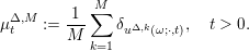
The convergence of this Monte Carlo algorithm to a statistical solution of (2.1) in the limit  ${\rm\Delta}\rightarrow 0$ and
 $M\rightarrow \infty$, will be shown in Fjordholm, Lye and Mishra (Reference Fjordholm, Lye and Mishra2016c).
10 Uncertainty quantification
10.1 What is uncertainty quantification?
Any PDE, such as systems of conservation laws (2.1), requires inputs such as the initial data, boundary conditions, flux coefficients and source terms. In practice, these inputs are obtained by some process of measurement. However, all measurements are inherently uncertain, that is, it is not possible to specify measured values exactly. These measurement errors lead to an intrinsic uncertainty in the inputs to a PDE, such as (2.1). These uncertainties are propagated by the solution map of the PDE and result in uncertainties in the corresponding solutions to the underlying PDE. The modelling, analysis and computation of these uncertain solutions falls under the rubric of uncertainty quantification (UQ).
UQ is a rapidly emerging interdisciplinary research area that spans applied mathematics, scientific computing, statistics and engineering. Although UQ involves various aspects in the modelling and computation of uncertainty, we focus here on the rather limited aspect of computational uncertainty propagation. Uncertainty propagation, also called forward UQ, refers to the computation of solutions of PDEs with uncertain inputs such as initial data, boundary conditions, coefficients and source terms. Given our focus on PDEs that model fluid dynamics, we shall discuss forward UQ in the limited context of systems of conservation laws (2.1). The reader is referred to Ghanem, Higdon and Owhadi (2016) for a comprehensive discussion of UQ in the context of elliptic, parabolic and linear hyperbolic PDEs.
10.2 UQ with random fields
As stated in Section 9, the most popular paradigm for UQ in the context of hyperbolic systems of conservation laws (2.1) has been to use random fields to model uncertain inputs as well as uncertain solutions. For simplicity of the exposition, we only consider the case where the initial data in (2.1) is uncertain. We let  $({\rm\Omega},{\mathcal{X}},\mathsf{P})$ denote a complete probability space and model the initial data
 $u_{0}$ as a random field, that is, a map
 $u_{0}:{\rm\Omega}\mapsto L^{1}(D)$ which is measurable with respect to the Borel
 ${\it\sigma}$-algebra
 ${\mathcal{B}}(L^{1}(D))$ Here,
 $D\subset \mathbb{R}^{d}$ denotes the spatial domain. The initial random field
 $u_{0}$ could be described in terms of a finite number of uncertain parameters or could be given in terms of a Karhunen–Loève expansion. Formally, the system of conservation laws (2.1) becomes
 $$\begin{eqnarray}\begin{array}{@{}rcl@{}}\partial _{t}u({\it\omega};x,t)+{\rm\nabla}_{x}\cdot f(u({\it\omega};x,t))\; & =\; & 0,\\ u({\it\omega};x,0)\; & =\; & u_{0}({\it\omega};x).\end{array}\end{eqnarray}$$
Following Mishra and Schwab (Reference Mishra and Schwab2012), we define a random entropy solution of (10.1) as follows.
Definition 10.1. A random field  $u:{\rm\Omega}\rightarrow C([0,T),L^{1}(D))$ is a random entropy solution of the uncertain system of conservation laws (10.1) if
 $u({\it\omega})$ satisfies (2.2) for almost every
 ${\it\omega}\in {\rm\Omega}$ as well as the entropy inequality (2.3) for almost every
 ${\it\omega}\in {\rm\Omega}$.
Thus, random entropy solutions are a pathwise (in  ${\rm\Omega}$) concept of solutions for the random conservation laws. Rigorous well-posedness results for random entropy solutions of (10.1) were obtained in the special case of scalar conservation laws in Mishra and Schwab (Reference Mishra and Schwab2012). The authors constructed this random entropy solution as simply specifying
 $$\begin{eqnarray}u({\it\omega};\cdot ,t)=\mathbf{S}_{t}u_{0}({\it\omega};\cdot ),\end{eqnarray}$$
where  $\mathbf{S}_{t}$ is the solution map defined in Theorem 2.4. Well-posedness results for the random entropy solutions for scalar conservation laws, but with uncertain fluxes, have also been obtained by Mishra, Risebro, Schwab and Tokareva (Reference Mishra, Risebro, Schwab and Tokareva2016). Since random entropy solutions are a pathwise concept, no well-posedness results for random entropy solutions have been obtained for (multi-dimensional) systems of conservation laws, on account of the lack of well-posedness results for the deterministic problem.
10.2.1 Computation of random entropy solutions
A large variety of numerical methods have been developed for UQ, particularly in the context of elliptic and parabolic PDEs. Some of them have been adapted, with varying degrees of success, to non-linear hyperbolic PDEs such as (10.1). We will provide a very brief survey of these methods, and refer readers to the book by Bijl et al. (2014) for a detailed discussion and comparison of these methods.
Stochastic Galerkin methods, based on generalized polynomial chaos, have been widely used in UQ for elliptic and parabolic problems (Ghanem and Spanos Reference Ghanem and Spanos1991). Some of these methods have been extended to compute random entropy solutions of (10.1), such as those in Després, Poëtte and Lucor (Reference Després, Poëtte and Lucor2009) and Tryoen, Le Maı̂tre, Ndjinga and Ern (Reference Tryoen, Le Maître, Ndjinga and Ern2010) and references therein. However, these methods suffer from the fact that they are intrusive: new code needs to be written and existing codes for solving (2.1) cannot be used directly. Furthermore, the lack of regularity in hyperbolic PDEs limits the use of these methods to problems that contain only a small number of uncertain parameters.
Stochastic collocation methods are non-intrusive deterministic alternatives to stochastic Galerkin methods (Xiu and Hesthaven Reference Xiu and Hesthaven2005). Variants of these methods have been developed, based on weak forms of the underlying PDE, such as the stochastic collocation finite volume methods of Mishra et al. (Reference Mishra, Risebro, Schwab and Tokareva2016); see also Abgrall and Congedo (Reference Abgrall and Congedo2013) and Barth (Reference Barth2013). These methods are also restricted to a low number of uncertain inputs.
Monte Carlo methods are also heavily used in the context of computation of random entropy solutions; see Bijl et al. (2014). It is well known that Monte Carlo methods converge at a slow rate of  $M^{-1/2}$, with
 $M$ being the number of Monte Carlo samples. Hence, more efficient variants of Monte Carlo (MC) methods have been designed. The most popular alternative in the context of computation of random entropy solutions is that of multi-level Monte Carlo (MLMC) methods, first proposed by Giles (Reference Giles2008) but adapted to the case of conservation laws by Mishra and Schwab (Reference Mishra and Schwab2012) and Mishra, Schwab and Šukys (Reference Mishra, Schwab and Šukys2012a, Reference Mishra, Schwab and Šukys2012b, Reference Mishra, Schwab and Šukys2013), and references therein. These methods have the advantage of being non-intrusive, simple to implement and parallelize, and are able to handle inputs with a very large number of uncertain inputs.
10.3 Issues with random entropy solutions
Although random entropy solutions are the most popular paradigm in the context of UQ for conservation laws, there are some drawbacks to this solution concept.
∙ Modelling input uncertainty in terms of random fields leads to ambiguity in how initial statistical information is parametrized. As mentioned in Section 9, one can choose different probability spaces on which the initial random field is defined, and obtain very different parametrizations of the same statistical information. Thus, lack of uniqueness appears to be generic to such descriptions.
∙ The most serious drawback of modelling with random fields lies in the fact that there are no existence and uniqueness results for random entropy solutions for systems of conservation laws. This is not surprising, as random entropy solutions are a pathwise concept, and there are no existence and uniqueness results for the entropy solutions of the underlying deterministic PDE, as explained in Section 2.
Furthermore, the extensive numerical evidence presented in Sections 7 and 8 strongly suggests that the measure-valued solutions of (2.1) may be non-atomic, even if the initial data are atomic. Hence, a data-to-solution map (such as
$\mathbf{S}_{t}$ in Theorem 2.4) which has been basis of construction of random entropy solutions (see, e.g., Mishra and Schwab Reference Mishra and Schwab2012), may not be available for multi-dimensional systems. Thus, a pathwise concept such as random entropy solutions is incompatible with these models.∙ All the rigorous convergence results for numerical methods for approximating random fields have been obtained in the scalar case (see Mishra and Schwab Reference Mishra and Schwab2012 for convergence of MC and MLMC methods). No rigorous convergence results are available for systems of conservation laws. In particular, it has been postulated in some articles, such as Mishra et al. (Reference Mishra, Schwab and Šukys2012a), that MC and MLMC methods converge once one assumes convergence in
$L^{1}$ for numerical approximations of the underlying deterministic problem. However, as demonstrated in this article, there appears to be no empirical convergence in $L^{1}$ for standard numerical approximations of multi-dimensional systems of conservation laws. Hence, the postulated convergence in Mishra et al. (Reference Mishra, Schwab and Šukys2012a) may not be true. This casts serious doubt on the validity of the random entropy solutions, computed with various existing methods.


Given the above considerations, there is plenty of scope for the development of new paradigms for uncertainty quantification of systems of conservation laws (and incompressible Euler equations) that replace random fields (and random entropy solutions) as the solution framework.
10.4 UQ with measure-valued and statistical solutions
Measure-valued solutions, as defined in Section 3.2, can serve as a framework for uncertainty quantification for systems of conservation laws (2.1). To be more specific, we consider the case of uncertain initial data modelled by an initial (non-atomic) Young measure  ${\it\sigma}_{x}$. This measure encodes all information about one-point statistics of the uncertain initial data. In particular, the one-point PDF of the data (if it exists) can specify this initial measure. Once the measure-valued solution
 ${\it\nu}_{x,t}$ is available, one can obtain moments such as the mean and variance as well as one-point PDFs (or cumulative distribution functions, CDFs) of the uncertain solution. The measure-valued solution can be approximated by using the Monte Carlo Algorithm 4.4. The convergence of this algorithm is guaranteed by Theorem 4.5. Thus, the existence of measure-valued solutions, as well as convergence of the Monte Carlo algorithms for computing them, has already been rigorously established. This should be seen in contrast to the random fields paradigm of UQ, where such results are lacking.
However, as described in the Section 9, the main drawback of using measure-valued solutions as a UQ framework lies in the fact that measure-valued solutions are non-unique, even in the scalar case, as soon as the initial data are non-atomic. As UQ requires non-atomic initial data, this non-uniqueness is generic when measure-valued solutions are used. Furthermore, measure-valued solutions provide no information on spatial correlations of the uncertain solutions. Both these defects may be remedied when one uses statistical solutions.
As described in Section 9, statistical solutions are time-parametrized probability measures on the underlying function space. They encode information about all possible spatial correlations of the underlying uncertain solution. Furthermore, statistical solutions do not contain any ambiguity in their parametrizations. If appropriate entropy conditions are found to enforce uniqueness of statistical solutions, then any parametrization (random field) corresponding to this unique statistical solution will lead to the same statistical solution. Given that statistical solutions can be computed using the Monte Carlo Algorithm 9.6, they offer a viable and robust framework for UQ for complex fluid flows.
11 Other algorithms for computing measure-valued solutions
In Sections 7 and 8 we demonstrated that the Monte Carlo-based ensemble-averaging Algorithms 4.1, 4.3 and 4.4 provide robust approximation to measure-valued solutions of the equations of inviscid fluid dynamics. However, as stated in Section 10, Monte Carlo algorithms have a slow rate of convergence of  $M^{-1/2}$ (Fjordholm et al. Reference Fjordholm, Käppeli, Mishra and Tadmor2016a, Appendix B). This slow convergence can impede the computational efficiency of these algorithms. Hence, there is a need for more efficient alternative algorithms for computing measure-valued solutions. We review some of them below.
11.1 A direct method
For simplicity, we consider systems of conservation laws (2.1) in one space dimension with initial data  $u_{0}$. We seek to compute measure-valued solutions of (2.1) with atomic initial data
 ${\it\sigma}_{x}={\it\delta}_{u_{0}(x)}$, and accomplish this by computing approximate solutions on a sequence of increasingly refined meshes. Let
 $u^{{\rm\Delta}_{x}}$ be corresponding approximate solutions, generated by the semi-discrete finite difference scheme (5.1a). We construct the following Young measure:
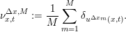 $$\begin{eqnarray}{\it\nu}_{x,t}^{{\rm\Delta}x,M}:=\frac{1}{M}\mathop{\sum }_{m=1}^{M}{\it\delta}_{u^{{\rm\Delta}x_{m}}(x,t)}.\end{eqnarray}$$
Here,  ${\rm\Delta}x_{m}$ indexes a sequence of mesh sizes and the
 $u^{{\rm\Delta}x_{m}}$ are numerical approximations generated by the finite difference scheme (5.1a). For instance, we can fix a
 ${\rm\Delta}x>0$ and set
 ${\rm\Delta}x_{m}=2^{-m}{\rm\Delta}x$.
One can readily adapt the proof of Theorem 5.1 to prove that the measure defined in (11.1) is a Young measure and (up to a subsequence) converges weak* to a measure-valued solution of (2.1), provided that the numerical scheme (5.1a) satisfies the conditions of Theorem 5.1. Thus, (11.1) provides a direct method for computing measure-valued solutions for atomic initial data. A similar method can be designed for several space dimensions. This algorithm has been considered by Laumer (Reference Laumer2014) and Mishra and Risebro (Reference Mishra and Risebro2016). Variants of this algorithm have also been considered by Glimm et al. (Reference Glimm, Grove and Zhang1999) and Lim et al. (Reference Lim, Yu, Glimm, Li and Sharp2008).
11.1.1 A numerical example
We illustrate the direct method with a numerical example reproduced from Laumer (Reference Laumer2014). He considers possibly the simplest situation where a non-atomic measure-valued solution can arise, even if the initial data are atomic. This is the so-called vanishing dispersion or KdV limit of the Burgers equation,
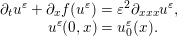 $$\begin{eqnarray}\begin{array}{@{}rcl@{}}\partial _{t}u^{{\it\varepsilon}}+\partial _{x}f(u^{{\it\varepsilon}})\; & =\; & {\it\varepsilon}^{2}\partial _{xxx}u^{{\it\varepsilon}},\\ u^{{\it\varepsilon}}(0,x)\; & =\; & u_{0}^{{\it\varepsilon}}(x).\end{array}\end{eqnarray}$$
Here,  $u^{{\it\varepsilon}}$ is a scalar function and the flux function
 $f$ is convex (concave) and of the form
 $f(u)=cu^{2}$ for some constant
 $c$. The characterization of the limit of
 $u^{{\it\varepsilon}}$ as
 ${\it\varepsilon}\rightarrow 0$ has been extensively studied, for instance in the pioneering works of Lax and Levermore (Reference Lax and Levermore1983a, Reference Lax and Levermore1983b, Reference Lax and Levermore1983c) and references therein. It was shown by DiPerna (Reference DiPerna1985) that this limit, corresponding to the Lax–Levermore construction, is a measure-valued solution of the underlying scalar conservation law. DiPerna provided a further characterization of the limit measure in terms of
 $k$-jets, corresponding to invariants of the KdV equation (DiPerna Reference DiPerna1985). In particular, the results of Lax and Levermore (Reference Lax and Levermore1983a), interpreted in the sense of DiPerna, reveal that the limit Young measure may be non-atomic even for atomic initial data. In fact, Lax and Levermore (Reference Lax and Levermore1983b) provide explicit solution formulas for the mean and the variance of the limit Young measure. These explicit formulas were the basis of a numerical method, designed by McLaughlin and Strain (Reference Mclaughlin and Strain1994), to compute the vanishing dispersion limit.
Direct method for the vanishing dispersion limit. The mean and the variance, at time  $t=0.15$, of the approximate measure-valued solution for the vanishing dispersion limit of the generalized Burgers equation (11.2), are computed with the direct method (11.1), based on the finite difference discretization of Laumer (Reference Laumer2014), and compared with the mean and the variance computed with the method of McLaughlin and Strain (Reference Mclaughlin and Strain1994). (a) Implicit Euler time-stepping, (b) Crank–Nicolson time-stepping. Both schemes use
 $M=100$ in (11.1).
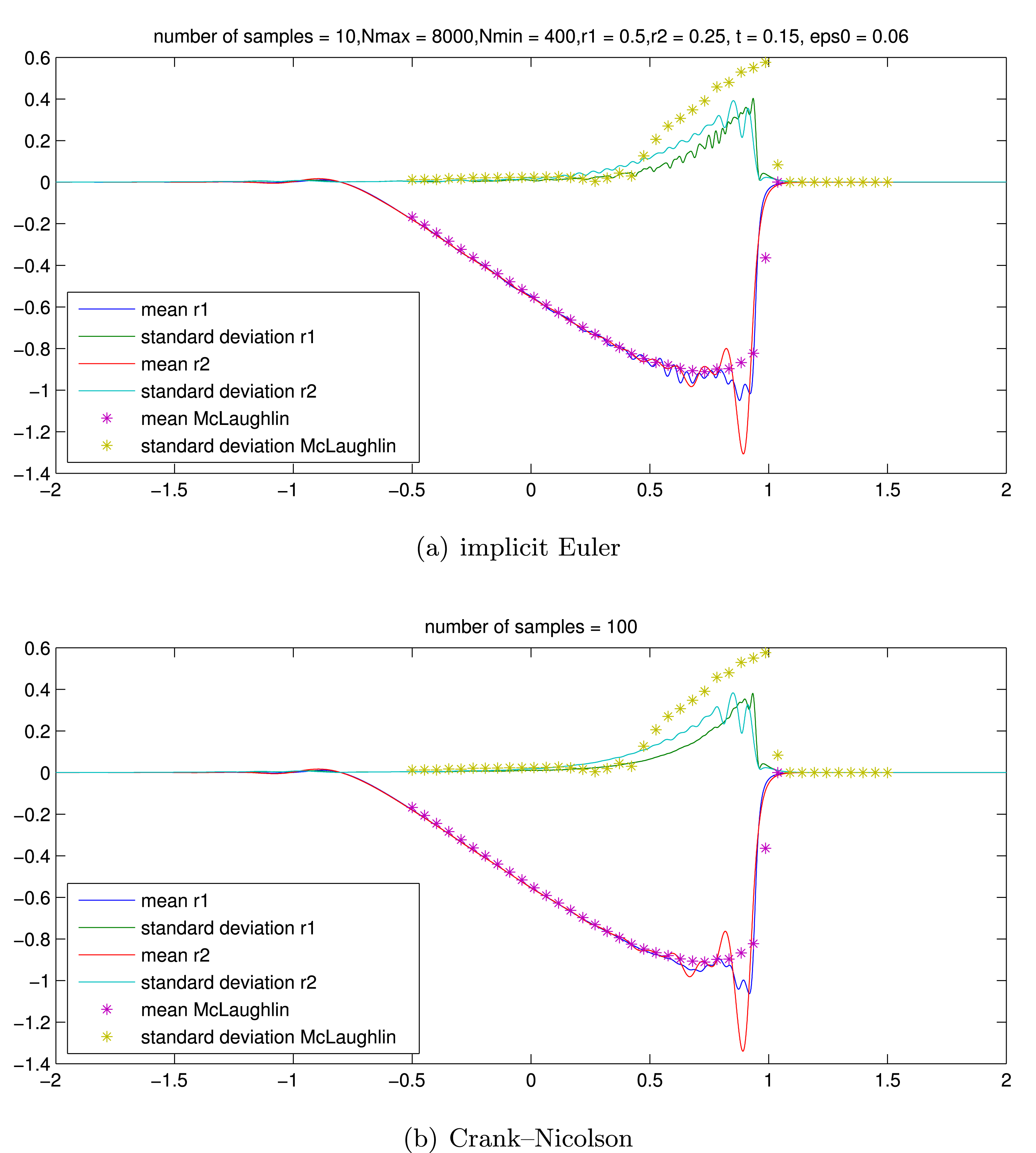
Laumer (Reference Laumer2014) used the aforementioned direct method to compute an approximate Young measure. More specifically, he discretized (11.2) with central finite difference spatial approximations and either implicit Euler or Crank–Nicolson time-stepping. Furthermore, he set  ${\it\varepsilon}=C{\rm\Delta}x$ as the (mesh-dependent) dispersion parameter. Both sets of schemes were proved to converge to a measure-valued solution of the scalar conservation law when
 ${\rm\Delta}x\rightarrow 0$. Furthermore, the direct method (11.1) and Algorithm 4.4, based on these schemes, were investigated in Laumer (Reference Laumer2014). Here we reproduce some representative results of Laumer (Reference Laumer2014). To this end, we consider a scalar conservation law with flux function
 $f(u)=-3u^{2}$ and fix the initial data
 $$\begin{eqnarray}\displaystyle u_{0}(x)=\left\{\begin{array}{@{}ll@{}}\displaystyle -\exp \biggl(\frac{1}{2}-\frac{1}{(2x+2)^{2}}-\frac{1}{(2x-2)^{2}}\biggr)\quad & \text{if}\quad |x|\leq 1,\\ 0\quad & \text{otherwise}.\end{array}\right. & & \displaystyle \nonumber\end{eqnarray}$$
We present results with the implicit finite difference discretization of Laumer (Reference Laumer2014) and the direct method for computing the measure-valued solution. The mean and the variance of (11.1) are plotted at time  $t=0.15$ in Figure 11.1, with
 $M=100$ and two different time discretizations: the implicit Euler scheme and the Crank–Nicolson scheme. The results are compared with the mean and the variance of the measure-valued solution of the Burgers equation that corresponds to the vanishing dispersion limit, with the method of McLaughlin and Strain (Reference Mclaughlin and Strain1994). This figure clearly shows that the results for the implicit Euler and Crank–Nicolson time-stepping schemes are nearly identical. Further, we make the following remarks.
∙ The measure-valued solution of the Burgers equation corresponding to the vanishing dispersion limit is non-atomic. The variance is clearly non-zero.
∙ The direct method (11.1) provides a fairly good approximation of the mean, even though some dispersive oscillations are observed.
∙ The approximation of the variance is much less accurate. There are large errors in the computation of the variance with (11.1) (with
$M=100$) if the McLaughlin–Strain solution is used as a reference solution.

In Figure 11.2 we present results for exactly the same set-up but with the perturbation-based Algorithm 4.3. To be more specific, we apply Algorithm 4.3 to the (generalized) Burgers equation with  $f(u)=-3u^{2}$ and with underlying implicit Euler and Crank–Nicolson centred finite difference discretization of (11.2), with
 ${\it\varepsilon}={\rm\Delta}x$. The results, for
 $100$ Monte Carlo samples, show the following.
Perturbation method for the vanishing dispersion limit. The mean and the variance, at time  $t=0.15$, of the approximate measure-valued solution for the vanishing dispersion limit of the generalized Burgers equation (11.2), are computed with Algorithm 4.3, based on the finite difference discretization of Laumer (Reference Laumer2014), and compared with the mean and the variance computed with the method of McLaughlin and Strain (Reference Mclaughlin and Strain1994). (a) Implicit Euler time-stepping, (b) comparison of implicit Euler and Crank–Nicolson time-stepping. Both schemes use
 $100$ Monte Carlo samples.
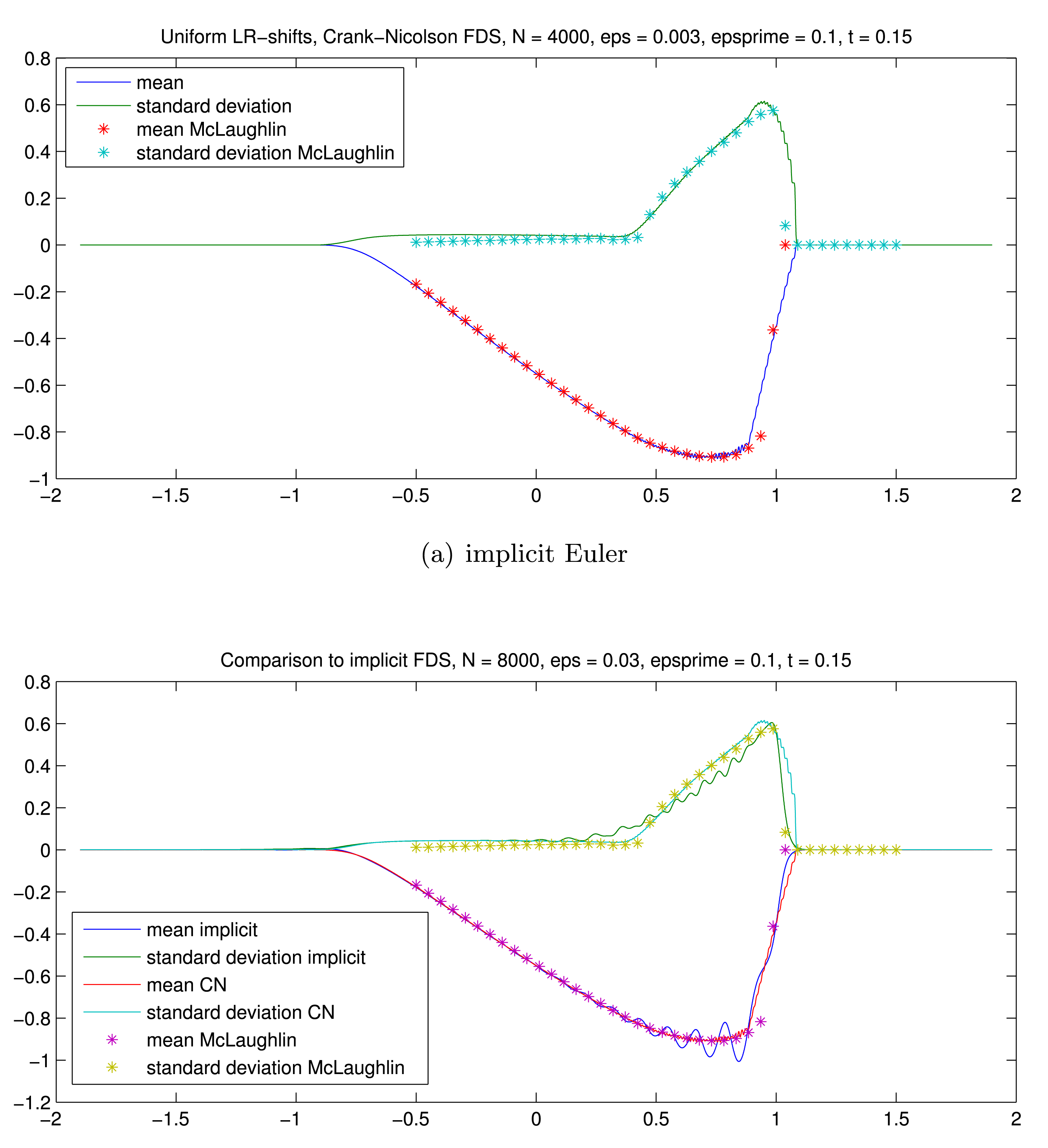
∙ The mean of the computed measure-valued solution is resolved very accurately. In particular, the Crank–Nicolson scheme (second-order time-stepping) resolves the mean in a non-oscillatory manner, whereas the mean, computed with the implicit Euler method, has some dispersive oscillations.
∙ The variance of the underlying Young measure is computed very accurately with both schemes. There is a slightly better resolution of the variance with the Crank–Nicolson scheme than with the implicit scheme.
Comparing Figures 11.1 and 11.2, we clearly see that the perturbation-based Algorithm 4.3 is more accurate than the direct method (11.1) at computing the underlying measure-valued solution. In particular, Laumer (Reference Laumer2014) observed that the computation of variance with Algorithm 4.3 was considerably more accurate than the direct method for the same computational cost.
Furthermore, using the direct method necessitates the use of very fine grids, as  $M$ in (11.1) must be high in order to provide accurate computation of statistics of the measure-valued solution. For instance, the results in Figure 11.1 were computed on a sequence of 100 grids ranging from 400 to 8000 mesh points. Even then, the numerical approximation of variance was not accurate enough, and even finer grid resolutions are necessary. Such fine grids are not feasible in two, let alone three, space dimensions. Thus, the direct method appears to be restricted to one-dimensional problems.
Mishra and Risebro (Reference Mishra and Risebro2016) consider the direct method applied to three-phase flow in a one-dimensional porous medium.
11.2 Multi-level Monte Carlo method
As mentioned earlier, the multi-level Monte Carlo (MLMC) method was introduced by Giles (Reference Giles2008) in order to speed up the slow convergence of the Monte Carlo algorithm. In the context of non-linear hyperbolic PDEs, it was adapted by Mishra and Schwab (Reference Mishra and Schwab2012) to approximate random entropy solutions of conservation laws. Further developments of the MLMC method in the context of hyperbolic problems are described in Mishra, Schwab and Šukys (Reference Mishra, Schwab and Šukys2012a, Reference Mishra, Schwab and Šukys2012b, Reference Mishra, Schwab and Šukys2013, Reference Mishra, Schwab and Šukys2016) and references therein. Considering its success in computing entropy solutions of conservation laws, can the multi-level Monte Carlo method be used to compute measure-valued solutions? This question is investigated by Lye and Mishra (Reference Lye and Mishra2016), who adapt a suitable variant of the MLMC method to compute entropy measure-valued solutions of systems of conservation laws (2.1). We present a brief summary of the method and results of Lye and Mishra (Reference Lye and Mishra2016) in the following.
We consider the system (2.1) with initial (possibly non-atomic) measure-valued data  ${\it\sigma}$, and propose the following MLMC algorithm to compute underlying entropy measure-valued solutions.
Algorithm 11.1. Let  ${\rm\Delta}=({\rm\Delta}x_{1},\ldots ,{\rm\Delta}x_{d})$ denote a grid size parameter and let
 $L\in \mathbb{N}$. Let
 ${\it\sigma}^{{\rm\Delta}}\in \mathbf{Y}(\mathbb{R}^{d},\mathbb{R}^{N})$ be the initial Young measure.
For  $l=1,\ldots ,L$:
- Step 1:
For some probability space
$({\rm\Omega},{\mathcal{X}},\mathsf{P})$, draw $M_{l}$ independent and identically distributed random fields $u_{0,1}^{l},\ldots ,u_{0,M_{l}}^{l}:{\rm\Omega}\times \mathbb{R}^{d}\rightarrow \mathbb{R}^{N}$, all with the same law ${\it\sigma}^{{\rm\Delta}}$.- Step 2:
For every
$k$ and fixed ${\it\omega}\in {\rm\Omega}$, use the finite difference scheme (5.1a) to numerically approximate the conservation law (2.1) with initial data $u_{0,k}^{l}({\it\omega})$ by setting $$\begin{eqnarray}\displaystyle u_{k}^{l}({\it\omega};\cdot ,t) & = & \displaystyle \mathbf{S}_{t}^{{\rm\Delta}_{l}}u_{0,k}^{l}({\it\omega}),\nonumber\\ \displaystyle \widetilde{u}_{k}^{l-1}({\it\omega};\cdot ,t) & = & \displaystyle \mathbf{S}_{t}^{{\rm\Delta}_{l-1}}u_{0,k}^{l}({\it\omega}),\nonumber\end{eqnarray}$$where
${\rm\Delta}_{l}=2^{L-l}{\rm\Delta}$.- Step 3:
Define the approximate measure-valued solution
(11.3)$$\begin{eqnarray}{\it\nu}_{L}^{{\rm\Delta}}:=\frac{1}{M_{0}}\mathop{\sum }_{k=1}^{M_{0}}{\it\delta}_{u_{k}^{0}}+\mathop{\sum }_{l=1}^{L}\frac{1}{M_{l}}\mathop{\sum }_{k=1}^{M_{l}}({\it\delta}_{u_{k}^{l}}-{\it\delta}_{\widetilde{u}_{k}^{l-1}}).\end{eqnarray}$$






Thus, the measure-valued solution is approximated on a nested sequence of grids, by drawing (possibly different numbers of) samples on each grids and using a ‘telescopic’ sum involving differences between successive grid resolutions.
Lye and Mishra (Reference Lye and Mishra2016) prove that the approximate measure-valued solutions generated by the MLMC Algorithm 11.1 converge to an entropy measure-valued solution of (2.1). The assumptions on the underlying numerical approximation are similar to those in Theorem 4.5. However, the key question of the MLMC algorithm is not whether it converges to a measure-valued solution but whether it is more efficient (faster) than the Monte Carlo Algorithm 4.4. To this end, the following error estimate was shown in Lye and Mishra (Reference Lye and Mishra2016):
 $$\begin{eqnarray}\Vert \langle {\it\psi},\langle {\it\nu}^{{\rm\Delta}}-{\it\nu}_{L}^{{\rm\Delta}},g\rangle \rangle \Vert _{L^{2}({\rm\Omega})}\leq \frac{C_{1}}{M_{0}^{1/2}}+\mathop{\sum }_{l=1}^{L}\frac{C_{2}}{M_{l}^{1/2}}\text{Var}(\langle {\it\psi},g(u^{l})-g(u^{l-1})\rangle ),\end{eqnarray}$$
for every  ${\it\psi}\in L^{1}(D,\mathbb{R}^{N})$ and
 $g\in C_{0}(\mathbb{R}^{N})$. Here,
 ${\it\nu}^{{\rm\Delta}}$ is the approximate Young measure generated by Algorithm 4.1 and
 $\text{Var}(X)$ refers to the variance of any random field
 $X$.
One observes from the above error estimate that the error with respect to the MLMC algorithm relies heavily on the variance between successive levels. In particular, if the variance decays as the grid resolution is increased, then one can choose fewer samples  $M_{l}$ on fine mesh resolutions and obtain a lower error. Choosing a low number of samples for fine mesh resolutions will considerably speed up the performance of the MLMC algorithm, as observed and proved for scalar conservation laws in Mishra and Schwab (Reference Mishra and Schwab2012) and for linear hyperbolic systems in Mishra et al. (Reference Mishra, Schwab and Šukys2016).
We check whether this variance between levels decays as the mesh is refined by a numerical example. We consider the same set-up as the Kelvin–Helmholtz problem considered in Section 7.2, and show the variance between successive levels in Figure 11.3(a). As shown in the figure, the variance between levels remains approximately constant as the mesh is refined. Hence, one has to choose (approximately) the same number of samples at every mesh resolution. Therefore, the MLMC algorithm cannot be expected to converge faster than the Monte Carlo Algorithm 4.4. This fact is verified in Figure 11.3(b), where we show the error for the mean (in  $L^{1}$) of the measure-valued solution of the Kelvin–Helmholtz problem for the compressible Euler equations, computed with the MLMC Algorithm 11.1, based on the TeCNO2 scheme. The figure compares the error (computed with respect to an MC reference solution) for Algorithm 4.4 on a
 $1024^{2}$ mesh with the error for the MLMC Algorithm 11.1, with a
 $1024^{2}$ resolution grid serving as the finest level of refinement. We vary the number of samples at the finest level of the MLMC grid (and the only level for the MC grid) by two orders of magnitude, and observe from Figure 11.3(b) that the error is more or less identical for the two approaches. This implies that an MLMC method has the same accuracy as the MC method only when the same number of samples are used at the finest grid resolution of the MLMC method as in the MC method. Thus, the computational complexity of MLMC is no better (in fact, slightly worse) than the MC algorithm. Results for the variance (omitted here) are analogous. This lack of speed-up for the MLMC algorithm should be contrasted with the significant gain in complexity with the MLMC method for either scalar conservation laws (Mishra and Schwab Reference Mishra and Schwab2012), one-dimensional systems (Mishra et al. Reference Mishra, Schwab and Šukys2012a) or multi-dimensional linear hyperbolic systems (Mishra et al. Reference Mishra, Schwab and Šukys2016).
Multi-level Monte Carlo Algorithm 11.1, used to compute the measure-valued solution for the Kelvin–Helmholtz problem for the compressible Euler equations, described in Section 7.2. (a) Variance of the difference in successive levels of mesh resolution ( $y$-axis) versus mesh resolution (
 $x$-axis). (b) Error in the mean (in
 $L^{1}$ with respect to a reference solution computed with a Monte Carlo simulation on a
 $2048^{2}$ grid with
 $2048$ samples) (
 $y$-axis) versus number of MLMC samples at the finest grid resolution of
 $1024^{2}$ (
 $x$-axis). Specifically,
 $E(M_{L})=\Vert \text{MLMC}(u,M_{L},1024)-\text{MC}(u,2048,2048)\Vert _{L^{1}(D)}$.
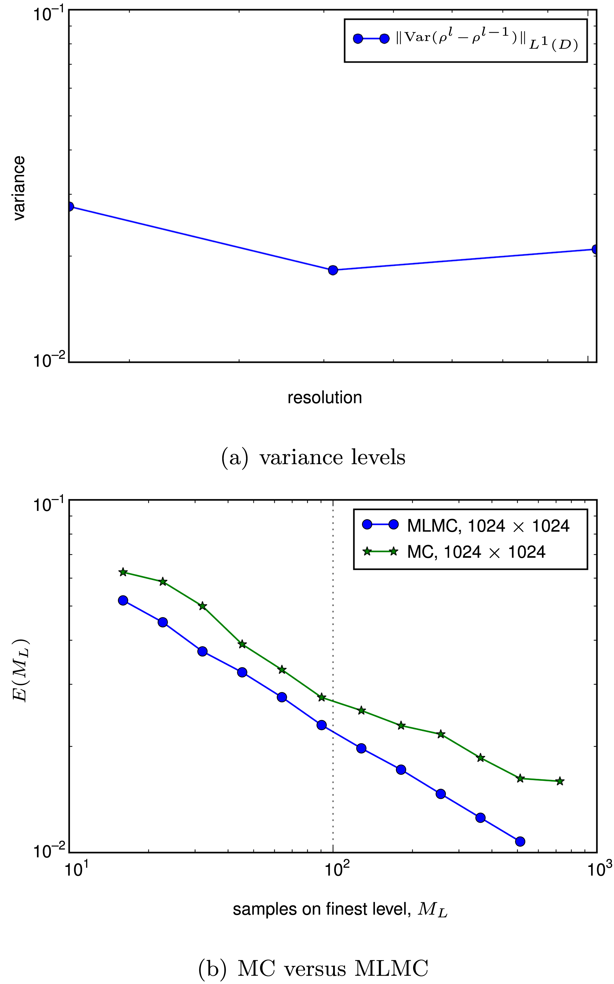
Stabilized version of the multi-level Monte Carlo Algorithm 11.1, used to compute the measure-valued solution for the Kelvin–Helmholtz problem for the compressible Euler equations, described in Section 7.2. (a) Variance of the difference in successive levels of mesh resolution ( $y$-axis) versus mesh resolution (
 $x$-axis). (b) Error in the mean (in
 $L^{1}$ with respect to a reference solution computed with a Monte Carlo simulation on a
 $2048^{2}$ grid with
 $2048$ samples) (
 $y$-axis) versus number of MLMC samples at the finest grid resolution of
 $1024^{2}$ (
 $x$-axis). Specifically,
 $E(M_{L})=\Vert \text{MLMC}(u,M_{L},1024)-\text{MC}(u,2048,2048)\Vert _{L^{1}(D)}$.
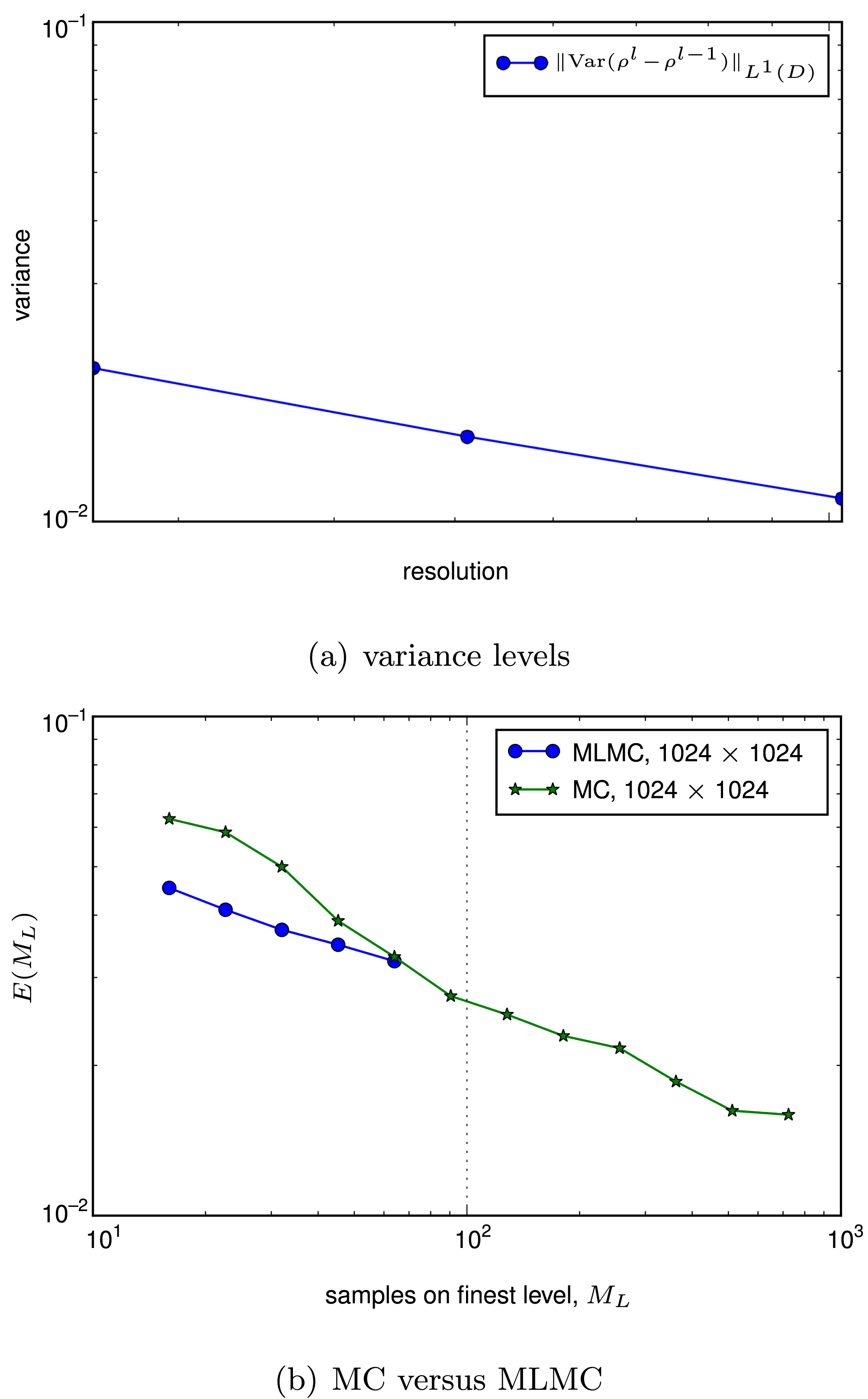
One possible remedy for the slow convergence of the MLMC algorithm was considered in Lye and Mishra (Reference Lye and Mishra2016), amounting to introducing a relaxation time. We fix  $T_{0}\approx 0.05$, and then we reset the coarse samples with the fine samples for every
 $t=nT_{0}$. In other words, we run the simulation between
 $t=(n-1)T_{0}$ and
 $t=nT_{0}$, and then we reset the coarse samples by
 $$\begin{eqnarray}\widetilde{u}_{k}^{l-1}({\it\omega};x,nT_{0})=u_{k}^{l}({\it\omega};x,nT_{0}).\end{eqnarray}$$
Since we observe short-time sample convergence (for instance in the case of the Kelvin–Helmholtz problem), this guarantees that
 $$\begin{eqnarray}\text{Var}(\langle {\it\psi},g(u^{l})-g(u^{l-1})\rangle )\leq C{\rm\Delta}^{s},\end{eqnarray}$$
as illustrated in Figure 11.4(a). However, by resetting the coarse samples, we introduce an error term of the form
 $$\begin{eqnarray}\mathop{\sum }_{l=0}^{L-1}|\langle {\it\psi},\langle {\it\nu}^{{\rm\Delta}x^{l}}-{\it\nu}^{{\rm\Delta}x^{l-1}},g\rangle \rangle |=O({\rm\Delta}_{0}^{s}).\end{eqnarray}$$
The error term is independent of the number of samples on each level, and scales as the coarsest spatial grid resolution. This can be clearly seen in Figure 11.4(b). Hence, even with this relaxation time approach, the MLMC Algorithm 11.1 is outperformed by the Monte Carlo Algorithm 4.4.
12 Young measures and their computation in other contexts
Young measures (and measure-valued solutions) arise in a variety of contexts other than fluid dynamics, particularly in elasticity and materials science. In particular, Young measures arise when one considers minimizers of non-convex variational problems. Indeed, recall that this was the original motivation behind the studies of L. C. Young (Reference Young1969). Such problems take the following generic form:
 $$\begin{eqnarray}\text{Find}~~u:=\text{arg min}_{u\in {\mathcal{A}}}\int _{D}Q(x,u,{\rm\nabla}u)\,\text{d}x.\end{eqnarray}$$
Here,  $u:D\subset \mathbb{R}^{d}\mapsto \mathbb{R}^{n}$ and
 ${\mathcal{A}}$ denotes a class of sufficiently smooth functions that incorporates the boundary conditions. In the context of elasticity,
 $u$ often denotes the deformation of the elastic material and
 $Q$ the stored elastic energy. As long as
 $Q$ is convex (quasi-convex in the vectorial case) in the last argument
 ${\rm\nabla}u$ (deformation gradient), one can use the direct method of calculus of variations (Dacarogna Reference Dacarogna1989) to calculate the minimizer that corresponds to the equilibrium state of the elastic material.
However, there are many models where  $Q$ need not be convex (resp. quasi-convex). These include optimal material design (Goodman, Kohn and Reyna Reference Goodman, Kohn and Reyna1986 and references therein) and micromagnetics (De Simone Reference De Simone1993 and references therein). The prototypical example of a non-convex variational problem is the modelling of the structure of crystalline materials (see Luskin Reference Luskin1996 and references therein). It is well known that crystals have two phases: a high-temperature homogeneous phase called austenite and a low-temperature, highly heterogeneous, phase called martensite. Martensitic materials contain many equilibrium phases, and crystal structure can alternate between these multiple phases. Hence, the popular models of the stored energy
 $Q$ in (12.1), such as the Eriksson–James model (Luskin Reference Luskin1996 and references therein), have a multiple well structure for
 $Q$.
Once the stored energy  $Q$ has a multiple well structure, the resulting variational problem is not convex (resp. quasi-convex). Hence, the direct method of calculus of variations is not applicable. Consequently, minimizing sequences may not converge under the strong topology of
 ${\mathcal{A}}$. Moreover, minimizing sequences consist of functions that oscillate between the multiple wells. Such functions contain oscillations at ever finer scales, suggesting the use of Young measures to describe the limit of such minimizing sequences. In fact, Young measures were originally introduced in this context: see Tartar (Reference Tartar1979) and Ball (Reference Ball, Rascle, Serre and Slemrod1989). Consequently, the variational problem (12.1) can be relaxed to:
 $$\begin{eqnarray}\begin{array}{@{}rcl@{}}\text{Find}~~(u,{\it\nu})\; & :=\; & \text{arg min}_{u\in {\mathcal{A}},{\it\nu}\in \mathbf{Y}}\int _{D}\langle {\it\nu}_{x},Q(x,u,\cdot )\rangle \,\text{d}x,\\ {\rm\nabla}u(x)\; & =\; & \langle {\it\nu}_{x},{\it\xi}\rangle ,\quad \text{for a.e }x\in D.\end{array}\end{eqnarray}$$
Here,  $u:D\mapsto \mathbb{R}^{n}\in {\mathcal{A}}$ is the deformation, with
 ${\mathcal{A}}$ denoting the admissible class of functions and
 $\mathbf{Y}=\mathbf{Y}(D,\,\mathbb{R}^{n\times n})$, the Young measure defined in Section 3.1. We do not specify
 ${\mathcal{A}}$ here as it depends on the modelling context and the boundary conditions. Note that the second equation in (12.2) specifies that
 ${\it\nu}$ is a gradient Young measure. In addition to the second equation in (12.2),
 ${\it\nu}$ has to satisfy some additional conditions for gradient Young measures (Kinderlehrer and Pedregal Reference Kinderlehrer and Pedregal1991).
The variational problem (12.2) has a solution, and this solution models observed crystalline structures such as laminates and microstructures, which involve high-frequency oscillations in material properties and sharp phase transitions between the austenite and martensite phases, as well as within various martensitic phases. The numerical approximation of (12.2) has been considered in many papers. We mention a very brief list of references here, and refer the reader to review papers such as Luskin (Reference Luskin1996) and Carstensen (Reference Carstensen2001) for further details.
There are two main approaches to computing solutions of the non-convex variational problem (12.2), as follows.
∙ Direct approximation of the Young measure. This approach was proposed by Nicolaides and Walkington (Reference Nicolaides and Walkington1993); see also Roubı́ček (Reference Roubíček1997) and references therein. It consists of approximating the gradient Young measure in (12.2) as a convex combination of Dirac masses. Such an approximation is motivated by the fact that crystalline phase transition, modelled by (12.2), oscillates between a finite number of phases. The locations of Dirac masses are uniformly distributed on a grid in phase space. Similarly, the admissible class
${\mathcal{A}}$ in (12.2) is approximated by a suitable piecewise polynomial finite element space. The resulting discrete variational problem comes with a large number of (non-linear) constraints that reflect that the fact that a gradient Young measure is approximated. This constrained finite-dimensional variational problem is solved using adapted optimization algorithms. This strategy appears to be robust at least for simple model problems in both one and two space dimensions (Nicolaides and Walkington Reference Nicolaides and Walkington1993).∙ A (quasi)-convexification approach. Another popular paradigm for solving (12.1) consists of (quasi)-convexifying the stored energy in (12.1), that is, replacing it with:
(12.3)Here,$$\begin{eqnarray}\text{Find}~~u:=\text{arg min}_{u\in {\mathcal{A}}}\int _{D}CQ(x,u,{\rm\nabla}u)\,\text{d}x.\end{eqnarray}$$$CQ$ refers to the convex (resp. quasi-convex in the vectorial case) envelope of the stored energy $Q$. Then, one restricts the admissible class to a finite element space and computes discrete minimizers. This approach has been considered by Collins and Luskin (Reference Collins and Luskin1989), Luskin (Reference Luskin1996) and Pedregal (Reference Pedregal1996). Luskin (Reference Luskin1996) presents a comprehensive review of error estimates for the approximate solutions with respect to the solution of the relaxed problem (12.3). Furthermore, a simple postprocessing step, such as one described in Carstensen (Reference Carstensen2001), recovers information about the Young measure in (12.2) from the minimizer of the discrete version of (12.3).However, the main problem with the quasi-convexification approach is the lack of explicit formulas for the quasi-convex envelopes for most stored energies that appear in practice; see Carstensen (Reference Carstensen2001) and references therein.




Both approaches to calculating the Young measure-valued solution of the non-convex variational problem (12.1) utilize deterministic approaches. It would be interesting to see whether the ensemble-based Monte Carlo algorithms, such as Algorithm 4.4, can be adapted to provide robust approximations of the non-convex variational problem (12.1).
Another context in which measure-valued solutions make an appearance is elastodynamics; see Demoulini et al. (Reference Demoulini, Stuart and Tzavaras2012) and references therein. Here, the governing equations can be written as systems of conservation laws (2.1). It has been hypothesized that the measure-valued solutions in elastodynamics are non-atomic, even for atomic initial data. The algorithms presented here, such as Algorithm 4.4, can be directly applied to numerical approximation of these models.
13 Conclusion
We have presented examples of PDEs where (admissible) weak solutions (integrable functions) may not be the appropriate solution framework, as revealed by state-of-the-art numerical approximations of these equations.
∙ The (approximate) solutions contain structures (oscillations) at ever finer spatial scales.
∙ These (approximate) solutions are not stable with respect to initial perturbations or changes in the numerical method.
The lack of global existence and uniqueness results for these PDEs may be attributed to these fine-scale oscillations and instabilities. They are also responsible for the lack of convergence (under mesh refinement) of standard numerical approximations for these equations. We have provided numerical experiments for the compressible, as well as incompressible, Euler equations to illustrate the aforementioned phenomena.
Given these considerations, we postulate that (admissible) measure-valued solutions, as first proposed by DiPerna (Reference DiPerna1985), are better suited to describing the unstable and highly oscillatory structure of the (approximate) solutions for these PDEs. Measure-valued solutions are Young measures, that is, space-time parametrized probability measures. We have provided a self-contained introduction to Young measures as well as to generalized Young measures. We have defined entropy (admissible) measure-valued solutions for systems of conservation laws (incompressible Euler equations) and presented some associated theoretical results.
The main focus of the current article has been to review an ensemble-averaging algorithm, proposed by Fjordholm et al. (Reference Fjordholm, Käppeli, Mishra and Tadmor2016a), for approximating a measure-valued solution. A generic form of this Monte Carlo-based algorithm has been presented, along with suitable modifications for atomic initial data. Specific details of the algorithm were provided for both systems of conservation laws and the incompressible Euler equations. In particular, we have shown that discretizations based on high-resolution finite volume and discontinuous Galerkin schemes for systems of conservation laws, and spectral as well as finite difference approximations for the incompressible Euler equations, converge to an admissible measure-valued solution.
We have presented a large number of numerical experiments that demonstrate the following.
∙ Approximate solutions generated by Algorithm 4.4 converge as the mesh is refined. This is in sharp contrast to the observed non-convergence of individual realizations (single samples) under mesh refinement.
∙ Statistical quantities of interest, such as mean, variance and one-point PDFs (CDFs), are computed robustly with Algorithm 4.4.
∙ The computed measure-valued solutions appear to be stable with respect to different numerical methods and different types of initial perturbations. Again, this should be compared with the instabilities of single samples.
∙ The computed measure-valued solution may be non-atomic, even when the underlying initial data form an atomic Young measure.
Given these observations, one can conclude that that measure-valued solutions offer a far more promising paradigm as solutions of the compressible/incompressible Euler equations than do entropy/admissible weak solutions. The Monte Carlo Algorithm 4.4, based on numerical discretizations that satisfy certain verifiable properties, provides an attractive framework for the robust computation of approximations to these PDEs.
However, the concept of measure-valued solutions (and their approximation) has its deficiencies. The main drawback of measure-valued solutions lies in the fact that measure-valued solutions are not necessarily unique, even for simple models such as scalar conservation laws, as shown in Example 9.1. We suggest that the concept of statistical solutions might overcome this defect of measure-valued solutions. As described in Section 9, statistical solutions are time-parametrized probability measures on a (problem-dependent) function space. These probability measures encode information about all possible spatial correlations and can be determined from their moments. Consequently, the moments of the probability measure must be evolved in time in a manner consistent with the original time-dependent PDE.
Young measures, and in particular measure-valued solutions, are the one-point correlation marginals of statistical solutions. Thus, statistical solutions contain a considerably greater amount of information than do measure-valued solutions. Suitable entropy conditions, such as those suggested by Fjordholm et al. (Reference Fjordholm, Lanthaler and Mishra2016b) for the case of scalar conservation laws, can ensure uniqueness of statistical solutions, even when the initial probability measure is non-atomic. Moreover, the ensemble-averaging Algorithm 9.6 can be employed to robustly compute statistical solutions. Hence, we postulate that statistical solutions are the appropriate solution paradigm for a large class of non-linear PDEs, such as systems of conservation laws (and incompressible Euler equations). Furthermore, statistical solutions serve as a proper framework for uncertainty quantification (UQ) for these models.
The key unresolved issue in the context of statistical solutions is the design of appropriate admissibility conditions that can ensure uniqueness and stability of statistical solutions for systems of conservation laws and incompressible Euler equations.
The Monte Carlo-based algorithms suggested here converge at a rate that scales as a reciprocal of the square root of the number of samples. This rather slow convergence can impede the efficiency of these algorithms, particularly for problems in three space dimensions. However, alternative algorithms such as the direct method, presented in Section 11, are not feasible for two- or three-dimensional computations. Surprisingly, the multi-level Monte Carlo (MLMC) method, successfully used to compute random entropy solutions of scalar conservation laws and linear hyperbolic systems in Mishra and Schwab (Reference Mishra and Schwab2012) and Mishra et al. (Reference Mishra, Schwab and Šukys2012a, Reference Mishra, Schwab and Šukys2012b, Reference Mishra, Schwab and Šukys2013, Reference Mishra, Schwab and Šukys2016), fails to be efficient for approximating measure-valued solutions. Consequently, MC algorithms are still the most suitable algorithms for computing measure-valued and statistical solutions. It would be interesting to see whether other UQ algorithms, such as the quasi-Monte Carlo method, stochastic Galerkin schemes or stochastic finite volume methods, can be successfully adapted to the computation of measure-valued and statistical solutions. The design of such algorithms is a topic of ongoing investigation.
In addition to the above issues, there are many possible directions in which the results of this article can be extended.
∙ The sufficient conditions for a scheme to guarantee convergence to measure-valued solutions, namely the weak BV bound (5.14) and the discrete entropy inequality (5.15), should be thought of as key guiding principles in the design of numerical methods for systems of conservation laws. They can serve a purpose similar to those served by the criteria of conservation, consistency and monotonicity for the design of convergent schemes for scalar conservation laws (Godlewski and Raviart Reference Godlewski and Raviart1991). We have presented examples of schemes that satisfy these criteria in Section 5. It would be interesting to examine whether other standard schemes, such as those based on WENO reconstructions or the spectral viscosity method (and suitable variants thereof), satisfy these criteria.
∙ In Section 12 we presented a concise discussion of different deterministic approaches for computing approximate measure-valued solutions that arise as solutions of non-convex variational problems in elasticity and materials science. It is an open question whether the Monte Carlo algorithms presented here in the context of computational fluid dynamics can be adapted to computation of the underlying Young measure for non-convex variational problems.
∙ DiPerna and Majda (Reference DiPerna and Majda1987a) surmised that Young measures and MV solutions could serve as an appropriate solution framework for a large class of non-linear PDEs that are characterized by lack of compactness. These include the Vlasov–Poisson, Vlasov–Maxwell and Yang–Mills equations. Little work has been done on this score, particularly in the context of numerical approximations. These equations provide a possible avenue for the application of the algorithms presented here.
Appendix: Proof of Theorem 3.12
Proof. The proof follows that of Alibert and Bouchitté (Reference Alibert and Bouchitté1997, Theorem 2.5) fairly closely. We may assume that  ${\mathcal{L}}(D)<\infty$; a diagonal argument will prove the result for general
 $D$. Furthermore, we will assume that
 $p=1$, as the generalization to
 $p>1$ is straightforward.
We define  $L^{n}\in {\mathcal{M}}_{+}(D\times \bar{B})$ by
 $$\begin{eqnarray}\langle L^{n},\,{\it\psi}\rangle =\int _{D}\int _{\mathbb{R}^{N}}\hat{{\it\psi}}(x,{\it\xi})\,\text{d}{\it\nu}_{x}^{n}({\it\xi})\,\text{d}x,\quad {\it\psi}\in C_{0}(D\times \bar{B}).\end{eqnarray}$$
Then  $\{L^{n}\}_{n}$ is bounded:
 $$\begin{eqnarray}\displaystyle |\langle L^{n},\,{\it\psi}\rangle | & = & \displaystyle \biggl|\int _{D}\int _{\mathbb{R}^{N}}{\it\psi}\biggl(x,\frac{{\it\xi}}{1+|{\it\xi}|}\biggr)(1+|{\it\xi}|)\,\text{d}{\it\nu}_{x}^{n}({\it\xi})\,\text{d}x\biggr|\nonumber\\ \displaystyle & \leq & \displaystyle \Vert {\it\psi}\Vert _{\infty }\biggl({\mathcal{L}}(D)+\int _{D}\langle {\it\nu}_{x}^{n},\,|{\it\xi}|\rangle \,\text{d}x\biggr)\leq C\Vert {\it\psi}\Vert _{\infty }.\nonumber\end{eqnarray}$$
Thus, there is a subsequence, still denoted  $L^{n}$, and an
 $L\in {\mathcal{M}}_{+}(D\times \bar{B})$ such that
 $L^{n}\overset{\ast }{\rightharpoonup }L$, that is,
 $$\begin{eqnarray}\int _{D}\int _{\mathbb{R}^{N}}\hat{{\it\psi}}(x,{\it\xi})\,\text{d}{\it\nu}_{x}^{n}({\it\xi})\,\text{d}x\rightarrow \int _{D\times \bar{B}}{\it\psi}(x,z)\,\text{d}L(x,z)\end{eqnarray}$$
for all  ${\it\psi}\in C_{0}(D\times \bar{B})$. In particular, setting
 ${\it\psi}(x,z)={\it\varphi}(x)\widetilde{f}(x,z)$, we get
 $$\begin{eqnarray}\int _{D}\int _{\mathbb{R}^{N}}{\it\varphi}(x)f(x,{\it\xi})\,\text{d}{\it\nu}_{x}^{n}({\it\xi})\,\text{d}x\rightarrow \int _{D\times \bar{B}}{\it\varphi}(x)\widetilde{f}(x,z)\,\text{d}L(x,z)\end{eqnarray}$$
for all  ${\it\varphi}\in C_{0}(D),~f\in C_{1}$.
By the disintegration theorem (Ambrosio, Gigli and Savaré Reference Ambrosio, Gigli and Savaré2005, Theorem 5.3.1), there is a measure  $\widetilde{{\it\lambda}}\in {\mathcal{M}}_{+}(D)$ and a Young measure
 $\widetilde{{\it\nu}}:D\rightarrow {\mathcal{P}}(\mathbb{R}^{N})$, such that
 $$\begin{eqnarray}\int _{D\times \bar{B}}{\it\psi}(x,z)\,\text{d}L(x,z)=\int _{D}\int _{\bar{B}}{\it\psi}(x,z)\,\text{d}\widetilde{{\it\nu}}_{x}(z)\,\text{d}\widetilde{{\it\lambda}}(x)\end{eqnarray}$$
for all  ${\it\psi}\in C_{0}(D\times \bar{B})$. Let
 $\widetilde{{\it\lambda}}=h{\mathcal{L}}+{\it\lambda}_{s}$ be the Lebesgue decomposition of
 $\widetilde{{\it\lambda}}$ with respect to Lebesgue measure
 ${\mathcal{L}}$, so that
 $h\in L^{1}(D)$ and
 ${\it\lambda}_{s}\in {\mathcal{M}}_{+}(D)$ is singular with respect to
 ${\mathcal{L}}$. For any
 ${\it\varphi}\in C_{0}(D)$, let
 ${\it\psi}\in C_{0}(D\times \bar{B})$ be defined by
 $\hat{{\it\psi}}(x,{\it\xi}):={\it\varphi}(x)$, or equivalently,
 ${\it\psi}(x,z)={\it\varphi}(x)(1-|z|)$. Then by (A.1) and (A.3),
 $$\begin{eqnarray}\displaystyle \int _{D}{\it\varphi}(x)\,\text{d}x & \equiv & \displaystyle \int _{D}\int _{\bar{B}}{\it\psi}(x,z)\,\text{d}\widetilde{{\it\nu}}_{x}(z)\,\text{d}\widetilde{{\it\lambda}}(x)\nonumber\\ \displaystyle & = & \displaystyle \int _{D}{\it\varphi}(x)\int _{\bar{B}}(1-|z|)\,\text{d}\widetilde{{\it\nu}}_{x}(z)\,\text{d}\widetilde{{\it\lambda}}(x)\nonumber\\ \displaystyle & = & \displaystyle \int _{D}{\it\varphi}(x)\int _{\bar{B}}(1-|z|)\,\text{d}\widetilde{{\it\nu}}_{x}(z)h(x)\,\text{d}x\nonumber\\ \displaystyle & & \displaystyle \qquad +\int _{D}{\it\varphi}(x)\int _{\bar{B}}(1-|z|)\,\text{d}\widetilde{{\it\nu}}_{x}(z)\,\text{d}{\it\lambda}_{s}(x).\nonumber\end{eqnarray}$$
Since this holds for all  ${\it\varphi}\in C_{0}(D)$, and since
 ${\mathcal{L}}$ and
 ${\it\lambda}_{s}$ are mutually singular, we can conclude the following.
∙ For
${\it\lambda}_{s}$-a.e. $x\in D$, Since$$\begin{eqnarray}\int _{\bar{B}}(1-|z|)\,\text{d}\widetilde{{\it\nu}}_{x}(z)=0.\end{eqnarray}$$$1-|z|\geq 0$ in $\bar{B}$ and $1-|z|=0$ if and only if $z\in S^{N-1}$, we find that $\widetilde{{\it\nu}}_{x}$ is supported on $S^{N-1}$ for ${\it\lambda}_{s}$-a.e. $x\in D$.∙ For
${\mathcal{L}}$-a.e. $x\in D$, (A.4)so$$\begin{eqnarray}h(x)\int _{\bar{B}}(1-|z|)\,\text{d}\widetilde{{\it\nu}}_{x}(z)=1,\end{eqnarray}$$$h(x)=(\int _{\bar{B}}(1-|z|)\,\text{d}\widetilde{{\it\nu}}_{x}(z))^{-1}$.



Therefore, (A.2) gives
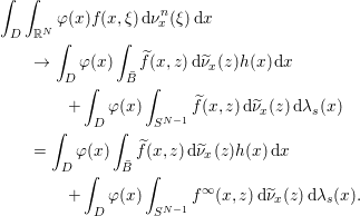 $$\begin{eqnarray}\displaystyle & & \displaystyle \int _{D}\int _{\mathbb{R}^{N}}{\it\varphi}(x)f(x,{\it\xi})\,\text{d}{\it\nu}_{x}^{n}({\it\xi})\,\text{d}x\nonumber\\ \displaystyle & & \displaystyle \qquad \rightarrow \int _{D}{\it\varphi}(x)\int _{\bar{B}}\widetilde{f}(x,z)\,\text{d}\widetilde{{\it\nu}}_{x}(z)h(x)\,\text{d}x\nonumber\\ \displaystyle & & \displaystyle \qquad \qquad +\int _{D}{\it\varphi}(x)\int _{S^{N-1}}\widetilde{f}(x,z)\,\text{d}\widetilde{{\it\nu}}_{x}(z)\,\text{d}{\it\lambda}_{s}(x)\nonumber\\ \displaystyle & & \displaystyle \qquad =\int _{D}{\it\varphi}(x)\int _{\bar{B}}\widetilde{f}(x,z)\,\text{d}\widetilde{{\it\nu}}_{x}(z)h(x)\,\text{d}x\nonumber\\ \displaystyle & & \displaystyle \qquad \qquad +\int _{D}{\it\varphi}(x)\int _{S^{N-1}}f^{\infty }(x,z)\,\text{d}\widetilde{{\it\nu}}_{x}(z)\,\text{d}{\it\lambda}_{s}(x).\end{eqnarray}$$
Introducing
 $$\begin{eqnarray}{\it\nu}_{x}^{\infty }:=\frac{1}{\widetilde{{\it\nu}}_{x}(S^{N-1})}\widetilde{{\it\nu}}_{x}\in {\mathcal{P}}(S^{N-1}),\quad {\it\lambda}:=\widetilde{{\it\nu}}_{x}(S^{N-1})h{\mathcal{L}}+{\it\lambda}_{s}\in {\mathcal{M}}_{+}(D)\end{eqnarray}$$
and rearranging, we find that
 $$\begin{eqnarray}\displaystyle \int _{D}\int _{\mathbb{R}^{N}}{\it\varphi}(x)f(x,{\it\xi})\,\text{d}{\it\nu}_{x}^{n}({\it\xi})\,\text{d}x & \rightarrow & \displaystyle \int _{D}{\it\varphi}(x)\int _{B}\widetilde{f}(x,z)\,\text{d}\widetilde{{\it\nu}}_{x}(z)h(x)\,\text{d}x\nonumber\\ \displaystyle & & \displaystyle \qquad +\int _{D}{\it\varphi}(x)\int _{S^{N-1}}f^{\infty }(x,z)\,\text{d}{\it\nu}_{x}^{\infty }(z)\,\text{d}{\it\lambda}(x).\nonumber\end{eqnarray}$$
Define  ${\it\nu}\in {\mathcal{M}}(D\times \mathbb{R}^{N})$ by
 $$\begin{eqnarray}\langle {\it\nu},\,g\rangle =\int _{D}\int _{B}\widetilde{g}(x,z)\,\text{d}\widetilde{{\it\nu}}_{x}(z)h(x)\,\text{d}x,\quad g\in C_{0}(D\times \mathbb{R}^{N})\end{eqnarray}$$
Then  ${\it\nu}$ can be disintegrated as
 $$\begin{eqnarray}\langle {\it\nu},\,g\rangle =\int _{D}\int _{\mathbb{R}^{N}}g(x,{\it\xi})\,\text{d}{\it\nu}_{x}({\it\xi})\,\text{d}x,\quad g\in C_{0}(D\times \mathbb{R}^{N})\end{eqnarray}$$
for a family of measures  ${\it\nu}_{x}\in {\mathcal{M}}_{+}(\mathbb{R}^{N})$. If
 $g(x,{\it\xi}):={\it\varphi}(x)$ for
 ${\it\varphi}\in C_{0}(D)$, then
 $g^{\infty }\equiv 0$, so (A.5) gives
 $$\begin{eqnarray}\displaystyle \int _{D}{\it\varphi}(x){\it\nu}_{x}(\mathbb{R}^{N})\,\text{d}x & = & \displaystyle \langle {\it\nu},\,g\rangle =\int _{D}{\it\varphi}(x)\int _{B}\widetilde{g}(x,z)\,\text{d}\widetilde{{\it\nu}}_{x}(z)h(x)\,\text{d}x\nonumber\\ \displaystyle & = & \displaystyle \int _{D}{\it\varphi}(x)\int _{B}(1-|z|)\,\text{d}\widetilde{{\it\nu}}_{x}(z)h(x)\,\text{d}x\nonumber\\ \displaystyle & = & \displaystyle \int _{D}{\it\varphi}(x)\,\text{d}x\quad \text{(by (A.4)).}\nonumber\end{eqnarray}$$
Hence,  ${\it\nu}_{x}(\mathbb{R}^{N})=1$ for a.e.
 $x\in D$, so
 ${\it\nu}$ is a Young measure.◻