
1. Introduction
In many problems of fluid dynamics, the Reynolds number is large and the flow structure is highly irregular – the localized velocity gradients may attain extreme values. This is a manifestation of strongly stretched and long-lived structures generated in narrow regions of the flow (Hunt, Wray & Moin Reference Hunt, Wray and Moin1988; Moisy & Jiménez Reference Moisy and Jiménez2004; Goto Reference Goto2008; Elsinga & Marusic Reference Elsinga and Marusic2010). The interaction of such structures leads to intense fluctuations of the energy dissipation rate, to violent accelerations of fluid particles and to long-range time auto-correlations (Mordant et al. Reference Mordant, Delour, Léveque, Arnéodo and Pinton2002). Recent direct numerical simulations (DNS) of homogeneous and isotropic turbulence (HIT), generated in a periodic box (the highest Taylor micro-scale Reynolds number  $Re_\lambda =1300$), performed by Yeung, Zhai & Sreenivasan (Reference Yeung, Zhai and Sreenivasan2015), Iyer, Sreenivasan & Yeung (Reference Iyer, Sreenivasan and Yeung2020) and Donzis, Yeung & Sreenivasan (Reference Donzis, Yeung and Sreenivasan2008) revealed that the velocity increments across the smallest turbulent length scales can be of the same order as that of the largest turbulent velocities in the flow. Such extreme velocity gradients imply also that molecular viscosity, or the local Reynolds number, plays a central role in the local structure of turbulence. So, the experimental measurements of Lagrangian statistics (Mordant, Crawford & Bodenschatz Reference Mordant, Crawford and Bodenschatz2004) showed that the increased Reynolds number induces stronger effects of intermittency.
In many natural phenomena and practical applications, we come across highly turbulent flow laden with evaporating droplets. Some examples of such flows include spray combustion in chemical propulsion systems, turbulent flows in stratocumulus clouds and spraying of pathogen-bearing droplets by violent exhalations. These two-phase flows are usually characterized by high Reynolds numbers. Therefore, it might be expected that the intermittent generation of intense fluid accelerations, mentioned above, may significantly affect the statistics of the droplet dynamics and evaporation. The problem is that the direct resolution of such accelerations is prohibitively costly. On the other hand, in large-eddy simulations (LES), the filter width is much larger than the smallest turbulent length scale and the contribution of subgrid scales (SGS) to a droplet's motion and evaporation needs to be modelled. In the vast majority of SGS models, the local structure of turbulence is assumed to be homogeneous, i.e. the gradients of the fluid flow variables in the vicinity of the droplet are estimated from filtered fields and not from their increments in the smallest turbulent motions on residual scales (Leboissetier, Okong'o & Bellan Reference Leboissetier, Okong'o and Bellan2005; Pera et al. Reference Pera, Réveillon, Vervisch and Domingo2006; Okong'o, Leboissetier & Bellan Reference Okong'o, Leboissetier and Bellan2008; Apte, Mahesh & Moin Reference Apte, Mahesh and Moin2009; Senoner et al. Reference Senoner, Sanjosé, Lederlin, Jaegle, García, Riber, Cuenot, Gicquel, Pitsch and Poinsot2009; Irannejad & Jaberi Reference Irannejad and Jaberi2014; Tsang, Trujillo & Rutland Reference Tsang, Trujillo and Rutland2014). This raises questions on how to account for SGS gradients in the fluid on the dynamics of evaporating droplets.
Among others, there are two approaches which address the intermittency effects on a heavy particle motion beyond the resolution domain of the LES. The first is based on the stochastic simulation of the fluid velocity gradients on residual scales, or of the fluid acceleration. The fluid velocity induced by that acceleration determines a Stokes drag of a heavy particle. In the second approach, while the LES formulation with standard closure models is retained, the main focus is put on the particle motion equation, in which the impact of the small-scale motions is taken into account as stochastic model. The LES–SSAM (stochastic subgrid acceleration model) pertains to the first approach. This model was first proposed by Sabel'nikov, Chtab & Gorokhovski (Reference Sabel'nikov, Chtab and Gorokhovski2007, Reference Sabel'nikov, Chtab and Gorokhovski2011) and was adapted for the wall-bounded flows by Zamansky, Vinkovic & Gorokhovski (Reference Zamansky, Vinkovic and Gorokhovski2013). Recently, LES–SSAM is revisited in Sabelnikov, Barge & Gorokhovski (Reference Sabelnikov, Barge and Gorokhovski2019). In Barge & Gorokhovski (Reference Barge and Gorokhovski2020), LES–SSAM is further developed for shear flows. In LES-SSAM, the filtered Navier–Stokes equations are locally driven by the stochastic force. In difference with other techniques for forcing the turbulence in physical space (see, for example, Palmore & Desjardins Reference Palmore and Desjardins2018, and references therein), the forcing in LES–SSAM is thought of as the local subgrid fluid acceleration with explicitly embedded statistical properties known from the measurements and DNS. Namely, the stochastic model of the subgrid fluid acceleration: (i) develops stretched tails with increasing the local Reynolds number, (ii) the decay of the time auto-correlation of the magnitude of acceleration is much slower than that of the components – consequently, the norm and the direction of acceleration are simulated in time by two statistically independent Ornstein–Uhlenbeck processes. The drawback of LES–SSAM is that the Langevin stochastic equations evolve locally in time, and not in space i.e. it is assumed that the two-point spatial correlation of the acceleration is determined by the filter width. The argument used to justify this suggestion is that in the theory of locally isotropic turbulence (Monin & Yaglom Reference Monin and Yaglom2013), the two-point auto-correlation of the fluid particle acceleration is short ranged. This notwithstanding, the two-point auto-correlation of the norm of acceleration may decay on much longer distances. For example, in Johnson & Meneveau (Reference Johnson and Meneveau2018) the LES velocity is complemented by its subgrid-scale component along the stochastic trajectories of a fluid particle. These trajectories are issued from the Lagrangian stochastic model for the velocity gradient tensor. Thus, the spatial correlations of sub-filter scale acceleration are introduced in Johnson & Meneveau (Reference Johnson and Meneveau2018). However, in this approach, the fields from the filtered Navier–Stokes equations are not modified by the modelled sub-filtered velocity gradients. Concerning the second approach, the Lagrangian simulation of stochastic trajectories in the flow laden by heavy particles, is addressed in Bini & Jones (Reference Bini and Jones2008). In this study, the instantaneous acceleration of a heavy particle is decomposed into two parts. The first part represents the acceleration resulting from response of the heavy particle to the filtered fluid velocity. The second part issues from the particle interaction with unresolved motions in the flow. This part is formulated as a delta-correlated Langevin force with the noise strength given by the local subgrid kinetic energy, i.e. mostly by resolved velocities. The model of Bini & Jones (Reference Bini and Jones2008) is discussed in § 3. A major concern with this model is that the effects of small-scale intermittency are disregarded in the particle dynamics. In LES–SDM (stochastic drag model) by Gorokhovski & Zamansky (Reference Gorokhovski and Zamansky2014, Reference Gorokhovski and Zamansky2018), these effects were explicitly included as sub-filtered acceleration of the particle, via modelling the energy dissipation rate ‘seen’ by the particle along its trajectory. Thereby, two models, for particles above and below the Kolmogorov length, were proposed in Gorokhovski & Zamansky (Reference Gorokhovski and Zamansky2014, Reference Gorokhovski and Zamansky2018). Recently, this idea was extended to bubbles dispersion in Zhang, Legendre & Zamansky (Reference Zhang, Legendre and Zamansky2019). Our concern with LES–SDM, as it stands, is twofold. First, LES–SDM was applied in the framework of one-way coupling. Its application with two-way coupling gives an additional advantage to generate the fluid sub-filtered acceleration, providing the spatial auto-correlation in the flow along the particle trajectory. Second, in order to avoid any negative or increasing with time auto-correlation functions, a more robust algorithm is needed for the particle acceleration direction. In the context of these comments, it is interesting to modify the droplet dispersion model from Gorokhovski & Zamansky (Reference Gorokhovski and Zamansky2014, Reference Gorokhovski and Zamansky2018) , and to assess it in the simulation of high Reynolds number flow on a relatively coarse mesh. The corresponding description of the model and its analysis is given in § 3 of this study.
Our second objective is to propose and assess a new stochastic SGS evaporation model for a droplet surrounded by the intermittent flow structures. The body of literature on numerical and experimental studies of turbulent evaporation is very large. The DNS for flows at a moderate Reynolds number with evaporating droplets, viewed as material inertial points were performed in different academic configurations (HIT by Mashayek (Reference Mashayek1998a), Reveillon & Demoulin (Reference Reveillon and Demoulin2007) and Weiss, Meyer & Jenny (Reference Weiss, Meyer and Jenny2018); homogeneous shear turbulence (HST) by Mashayek (Reference Mashayek1998b) and Weiss et al. (Reference Weiss, Giddey, Meyer and Jenny2020); mixing layers between two adiabatic slip walls by Miller & Bellan (Reference Miller and Bellan1999) and Okong'o & Bellan (Reference Okong'o and Bellan2004)). These simulations provided valuable insights into the role of the gas phase turbulence on the evaporation process. It is generally recognized that the turbulent transport of scalars supports evaporation, and due to the turbulence, the evaporation increases the total range of droplet sizes. In HIT, the evolution of the probability density function (p.d.f.) of the vapour mass fraction is controlled by the ratio between characteristic times of turbulent mixing and evaporation. In HST, the persisting orientation of inclined longitudinal vortex structures induces anisotropy in the fluctuations of the vapour mass fraction across all spectra of turbulent length scales, down to very small length scales. A considerable attention in DNS is also paid to effects of droplet clustering on the evaporation rate. The clusters of droplets is the result of interaction between droplet inertia and fluid acceleration seen by the droplets in turbulent structures (see, e.g. Toschi & Bodenschatz Reference Toschi and Bodenschatz2009). In the case of evaporating droplets, clusters are characterized by elevated vapour mass fractions. Therefore, the evaporation rate in clusters is low and it can be even prematurely halted if the vapour concentration reaches the saturation level. Recently, DNS was performed by Dalla Barba & Picano (Reference Dalla Barba and Picano2018) for turbulent air–acetone vapour jet ( $Re_{\lambda } = 77$) which carries small evaporating acetone droplets (initially, of
 $6\,\mathrm {\mu }\textrm {m}$). This DNS emphasized the significant role of dry air entrainment on the overall evaporation process. The turbulent vaporization was also the subject of recent experimental studies. These studies have significantly improved our understanding of the process. So, in Méès et al. (Reference Méès, Grosjean, Marié and Fournier2020), the digital holography of tracking a single
 ${\sim }100\,\mathrm {\mu }\textrm {m}$ droplet, moving and evaporating in HIT, showed that the intense fluctuations of the evaporation rate are connected to ‘jumps’ of the relative velocity between droplet and fluid. Thus the intermittency in the fluid is manifested along the droplet trajectory. Measurements in a poly-dispersed spray of evaporating water droplets carried by air jet flow (Sahu, Hardalupas & Taylor Reference Sahu, Hardalupas and Taylor2016) support a similar conclusion: the evaporation rate is strongly controlled by instantaneous fluctuations of the relative velocity. Two modes of turbulent evaporation were observed: the internal group slow evaporation in a droplet cluster, typically near the spray centre, and the single droplet intense evaporation, typically near the spray boundary. These experimental studies, along with the experimental study of Verwey & Birouk (Reference Verwey and Birouk2017), also support the earlier conclusion from experiments in Wu, Liu & Sheen (Reference Wu, Liu and Sheen2001), Hiromitsu & Kawaguchi (Reference Hiromitsu and Kawaguchi1995) and Birouk & Gökalp (Reference Birouk and Gökalp2006) that increasing the turbulence intensity promotes evaporation of droplets. In De Rivas & Villermaux (Reference De Rivas and Villermaux2016) and Villermaux et al. (Reference Villermaux, Moutte, Amielh and Meunier2017), the evaporation rate in layers of liquid droplets at very small Stokes number is described through analogy with scalar mixing (Villermaux Reference Villermaux2019). Those layers are referred to as spray lamellae. The evaporation process is considered as the mutual action of two sub-processes. The first is the continuous stretching of a spray lamella by shear stresses. The second is the diffusion of the saturated vapour to the dry ambience due to evaporation of outer droplets in lamellae. A net transport of mass resulting from this diffusion (in terms of Stefan's flow on the lamella border) and the stretching effect reduce the lamella thickness. The time when this thickness shrinks to zero is defined as the time scale of evaporation. The important conclusion, supported by experimental observations in this study, is that the evaporation time scale decreases in proportion to the amount of stretching. Steeper scalar gradients on the lamella border enhance the vaporization rate of outer droplets in lamella. This promotes the dilution of saturated vapour with air around the inner droplets. These latter vaporize. In addition to above mentioned experiments, the measurements from Sommerfeld & Qiu (Reference Sommerfeld and Qiu1998) and the measurements from an engine combustion network (Idicheria & Pickett Reference Idicheria and Pickett2007; Payri et al. Reference Payri, Viera, Wang and Malbec2016) provided abundant experimental data for high-speed injection of evaporating droplets in high turbulent Reynolds number conditions in the gas. These experiments are well controlled and, due to their simple geometry, they are good test cases for modelling.
In our work, we proposed and assessed two new stochastic models, one for droplet dispersion and the other for droplet evaporation in unresolved turbulent motions. The models comprise the intermittency effects in the local structure of the flow, and this is the novelty of proposed models. The structure of the paper is as follows. The LES equations are formulated in § 2. In § 3 the new stochastic models for the droplet motion are described and illustrated. Section 4 is devoted to the new stochastic model for droplet turbulent evaporation. In § 5, the proposed models are assessed and characterized in comparison with other stochastic models and with experimental observations of the turbulent spray evaporation. Also, further discussions are provided in this section. Section 6 concludes the current study.
2. Governing equations for fluid phase – LES
In LES, any flow variable  $\psi (\boldsymbol {x},t)$, defined in a domain
 $\varOmega$, is decomposed as
 $\psi = \bar {\psi } + \psi '$ where
 $\bar {\psi }$ is a filtered in space (resolved) variable,
 $\bar {\psi }(\boldsymbol {x},t) = \int _{\varOmega } \psi (\boldsymbol {x'},t)\varPsi _\varDelta (\boldsymbol {x}-\boldsymbol {x}')\,{\textrm {d}\kern0.7pt x}'$,
 $\varPsi _\varDelta (\boldsymbol {x})$ is a filter function (weight function) and
 $\varDelta$ is the filter width (usually a measure of the grid spacing). In variable density flows, the Favre, or density weighted, filtering is often introduced by
 $\bar {\rho }\tilde {\psi }(\boldsymbol {x},t) = \overline {\rho \psi } = \int _{\varOmega } \rho \psi (\boldsymbol {x'},t) \varPsi _\varDelta (\boldsymbol {x}-\boldsymbol {x}')\,{\textrm {d}\kern0.7pt x}'$. In the context of Euler–Lagrangian modelling of turbulent sprays, an individual liquid droplet is usually considered as a point source, assuming that the droplet size is much smaller than the resolved turbulent length scales in the fluid. Therefore, the local contributions from droplets are presented formally by local source terms in the Navier–Stokes equations. In LES, each droplet is interacting with the filtered velocity field, which, compared with the original field, contains fewer high frequencies. In order to evaluate the singular contribution from a droplet at its position
 $\boldsymbol {x}=\boldsymbol {x}'$, the delta function is replaced by
 $\delta (\boldsymbol {x}-\boldsymbol {x}')|_{\boldsymbol {x}=\boldsymbol {x}'} \sim 1/\varDelta ^3$. Therefore, the source terms in the filtered Navier–Stokes equations represent the volume average of individual contributions from droplets which visited a considered volume
 $\varDelta ^3$ at a given time instance. Applying the filtering operation to the Navier–Stokes equations, and using the Smagorinsky eddy-viscosity model, leads to the following transport equation for the filtered momentum
 $\bar {\rho }\tilde {u}_i$:
 \begin{equation} \frac{\partial \bar{\rho}\tilde{u}_i}{\partial t} + \frac{\partial \bar{\rho}\tilde{u}_i\tilde{u}_j}{\partial x_j} = \frac{\partial}{\partial{x_j}} \left( 2\bar{\rho} (\nu + \nu_{sgs}) \left[ \tilde{S}_{ij} - \frac{1}{3} \tilde{S}_{kk} \right] \right) - \frac{\partial \tilde{p}}{\partial x_i} + \tilde{S}_{mom,i}, \end{equation}
where  $\nu _{sgs}$,
 $\tilde {p}$,
 $\bar {\rho }$ and
 $\nu$ are the eddy viscosity, filtered pressure, filtered total fluid density and viscosity respectively,
 \begin{equation} \tilde{S}_{ij} = \frac{1}{2}\left[\frac{\partial \tilde{u}_i}{\partial x_j} + \frac{\partial \tilde{u}_j}{\partial x_i} \right] \end{equation}
is the rate of filtered strain tensor,  $\delta _{ij}$ is the Kronecker delta and
 $\tilde {S}_{mom,i}$ represents the
 $i$th component of the source term from the volume-average momentum of droplets located in the considered computational cell. Assuming the gaseous phase to be a perfect gas with multiple species, the filtered mass fraction of any given species
 $m$ (i.e.
 $\tilde {Y}_m$) is given by following expression:
 \begin{equation} \frac{\partial \bar{\rho}\tilde{Y}_m}{\partial t} + \frac{\partial \bar{\rho}\tilde{Y}_m\tilde{u}_j}{\partial x_j} = \frac{\partial}{\partial{x_j}} \left( \bar{\rho}\left[ D + \frac{\nu_{sgs}}{Sc_T} \right] \frac{\partial \tilde{Y}_m}{\partial {x_j}} \right) + \tilde{S}_{vap}\delta_{m1}. \end{equation}
Here,  $D$ is a single diffusion coefficient,
 $Sc_T$ is the subgrid Schmidt number, the first species (with index
 $m=1$ in the Dirac delta function of the last term) represents the liquid vapour generated by evaporating spray droplets and
 $\tilde {S}_{vap}$ is the volume-average source of the vapour mass issued from all droplets located in the considered computational cell. For the filtered total fluid density
 \begin{equation} \frac{\partial \bar{\rho}}{\partial t} + \frac{\partial \bar{\rho}\tilde{u}_j}{\partial x_j} = \tilde{S}_{vap}. \end{equation}
For the filtered total energy  $\bar {\rho } \tilde {e}$
 \begin{equation} \frac{\partial \bar{\rho}\tilde{e}}{\partial t} + \frac{\partial \bar{\rho}\tilde{e}\widetilde{u_j}}{\partial x_j} = \frac{\partial}{\partial{x_j}} \left(\left[ \frac{K}{\bar{\rho} c_p}+ \frac{\nu_{sgs}}{Pr_T} \right] \frac{\partial \tilde{e}}{\partial {x_j}} \right) - \frac{\partial \bar{p} \tilde{u}_j}{\partial x_j} + \frac{\partial \tilde{\tau}_{ij} \tilde{u}_j}{\partial x_j} + \tilde{S}_{energy}, \end{equation}
where  $K$ is the thermal conductivity,
 $Pr_T$ is the subgrid Prandtl number,
 $\tau _{ij} = 2\bar {\rho } (\nu + \nu _{sgs} )[ \tilde {S}_{ij} - \tilde {S}_{kk}/3]$ is the filtered viscous stress and
 $\tilde {S}_{energy}$ is the collective energy exchange with all droplets located in a considered computational cell. The temperature of the gaseous flow is then computed from the energy using the equation of state relations for perfect gas. The SGS turbulent viscosity is modelled using the one-equation eddy-viscosity model (Yoshizawa & Horiuti Reference Yoshizawa and Horiuti1985), in which the eddy viscosity is given from the integration of additional transport equation for the subgrid turbulent kinetic energy (TKE)
 $K_{sgs}$ for single-phase flows. Then
 $S_{p,sgs}$ is added to this transport equation in order to represent the rate at which the fluctuating components of the gas velocity are doing work in dispersing the spray droplets as shown in (2.6). The values for the model constants are same as in the earlier studies of Tsang et al. (Reference Tsang, Trujillo and Rutland2014) i.e.
 $C_l =1.048$ and
 $C_k = 0.094$
 \begin{gather} \frac{\partial \bar{\rho}K_{sgs}}{\partial t} + \frac{\partial \bar{\rho}K_{sgs}\tilde{u}_j}{\partial x_j} = \frac{\partial}{\partial{x_j}} \left( 2\bar{\rho} (\nu + \nu_{sgs}) \frac{\partial K_{sgs}}{\partial x_j} \right) + \tilde{\tau}_{ij} \tilde{S}_{ij} - C_l \bar{\rho} \frac{K_{sgs}^{3/2}}{\varDelta} +S_{p,sgs}, \end{gather}
 \begin{gather} \nu_{sgs} = C_k \varDelta K_{sgs}^{1/2}. \end{gather}
In this work, in equations (2.1)–(2.6), the filtered source terms due to droplets are replaced by stochastic source terms simulated as stochastic processes along the droplets trajectory
 \begin{gather} \frac{\partial \bar{\rho}\tilde{u}_i}{\partial t} + \frac{\partial \bar{\rho}\tilde{u}_i\tilde{u}_j}{\partial x_j} = \frac{\partial}{\partial{x_j}} \left( 2\bar{\rho} (\nu + \nu_{sgs}) \left[ \tilde{S}_{ij} - \frac{1}{3} \tilde{S}_{kk} \right] \right) - \frac{\partial \tilde{p}}{\partial x_i} + S_{mom,i}^{stoch}, \end{gather}
 \begin{gather} \frac{\partial \bar{\rho}\tilde{Y}_m}{\partial t} + \frac{\partial \bar{\rho}\tilde{Y}_m\tilde{u}_j}{\partial x_j} = \frac{\partial}{\partial{x_j}} \left( \bar{\rho}\left[ D + \frac{\nu_{sgs}}{Sc_T} \right] \frac{\partial \tilde{Y}_m}{\partial {x_j}} \right) + S_{vap}^{stoch}\delta_{m1}, \end{gather}
 \begin{gather} \frac{\partial \bar{\rho}}{\partial t} + \frac{\partial \bar{\rho}\tilde{u}_j}{\partial x_j} = S_{vap}^{stoch}, \end{gather}
 \begin{gather} \frac{\partial \bar{\rho}\tilde{e}}{\partial t} + \frac{\partial \bar{\rho}\tilde{e}\widetilde{u_j}}{\partial x_j} = \frac{\partial}{\partial{x_j}} \left(\left[ K + \frac{\bar{\rho} c_p \nu_{sgs}}{Pr_T} \right] \frac{\partial \tilde{T}}{\partial {x_j}} \right) - \frac{\partial \bar{p} \tilde{u}_j}{\partial x_j} + \frac{\partial \tilde{\tau}_{ij} \tilde{u}_j}{\partial x_j} + S_{energy}^{stoch}, \end{gather}
 \begin{gather} \frac{\partial \bar{\rho}K_{sgs}}{\partial t} + \frac{\partial \bar{\rho}K_{sgs}\tilde{u}_j}{\partial x_j} = \frac{\partial}{\partial{x_j}} \left( 2\bar{\rho} (\nu + \nu_{sgs}) \frac{\partial K_{sgs}}{\partial x_j} \right) + \tilde{\tau}_{ij} \tilde{S}_{ij} - C_l \bar{\rho} \frac{K_{sgs}^{3/2}}{\varDelta} +S_{p,sgs}^{stoch}. \end{gather}
The expressions for these source terms and the appropriate stochastic models are presented in the next section.
3. Stochastic models for droplet dispersion
3.1. Stochastic drag models of Wang & Squires and Bini & Jones
In the simulation of flows laden with small droplets or particles, it is common to associate the particle acceleration with a Stokes drag. Accordingly, in LES, the particle acceleration is usually expressed by its response time  $\tau _p = \rho _p d_p^2/18\rho \nu$ to the filtered flow velocity ‘seen’ at the position of the particle
 \begin{equation} \frac{\textrm{d}u_{p,i}}{\textrm{d}t} = \frac{\tilde{u}_i- u_{p,i}}{\tau_p}, \end{equation}
where  $\boldsymbol {u_{p}}$ is the particle velocity vector. As outlined in the review of Pozorski & Apte (Reference Pozorski and Apte2009), several stochastic models have been formulated over time for accounting in (3.1) for the subgrid fluctuations of the fluid velocity. Among these approaches, the model of Wang & Squires (Reference Wang and Squires1996) is the most simple and widely used. By analogy with Amsden, O'Rourke & Butler (Reference Amsden, O'Rourke and Butler1989) for turbulent dispersion of sprays in Reynolds-averaged Navier–Stokes (RANS) simulations, Wang & Squires (Reference Wang and Squires1996) supplemented the filtered fluid velocity (i.e.
 $\tilde {u}$) by a residual scale velocity
 $u'$, which is sampled once over a turbulent time scale
 $\tau _t$ (given by (3.2)), from a Gaussian distribution with a variance defined by the magnitude of local
 $K_{sgs}$
 \begin{equation} \tau_t = \min \left[\frac{K_{sgs}}{\varepsilon_\varDelta}, 0.162 \cdot \frac{K_{sgs}^{3/2}}{\varepsilon_{\varDelta}|\boldsymbol{\tilde{u}} - \boldsymbol{u_p}|}\right]. \end{equation}
Here,  $\varepsilon _{\varDelta }=C_l ({K_{sgs}^{3/2}}/{\varDelta })$ represents the locally resolved dissipation rate. When the small-scale properties of turbulence are influenced by events of extreme fluctuations, the acceleration of a heavy particle may be additionally governed by the force which would act in the fluid in the absence of the particle, i.e. by the fluid acceleration at the particle position. The contribution of the latter is simulated in Bini & Jones (Reference Bini and Jones2009) by Langevin stochastic force
 \begin{equation} \frac{\textrm{d}u_{p,i}}{\textrm{d}t} = \frac{\tilde{u}_i- u_{p,i}}{\tau_p} + b \delta_{ij}\,\textrm{d}W_j. \end{equation}
Here,  $\delta _{ij}\,\textrm {d}W_j, (\,j=1,2,3)$ represents the three-dimensional isotropic Wiener process, and the coefficient
 $b= (K_{sgs}/\tau _t)^{1/2}$ is linked to a typical time
 $\tau _t$ required for a droplet to traverse through a notional ‘unresolved eddy’. Two alternative expressions are considered in Bini & Jones (Reference Bini and Jones2009):
 $\tau _t = \varDelta /(u_{p,i}u_{p,i})^{1/2}$ and
 $\tau _t = \varDelta /(K_{sgs})^{1/2}$. Our motivation for further development of the stochastic motion equation for the particle is as follows. If the filter width
 $\varDelta$ is taken to be in the inertial interval of turbulence,
 $L\gg \varDelta \gg \eta$, then in LES approach the subgrid fluctuations of the velocity are assumed to be much smaller than the resolved velocities (in contrast to the velocity gradient, which is stronger on residual scales than one on the resolved scales). This underestimates the role of residual scales on the particle dispersion. Therefore, it would be preferable to characterize the norm of the Langevin force in (3.3) by a variable based on the subgrid velocity gradient (or subgrid acceleration), rather than on the turbulent velocity itself from
 $K_{sgs}$. This allows us to introduce another desirable statistical feature for this stochastic term, that is the Reynolds number dependency. Compared with the estimate in (3.3) of the resolved flow acceleration
 $a_\varDelta$ (given by variables such as
 $K_{sgs}$,
 $\varepsilon _\varDelta$,
 $\tau _t$), the unresolved flow acceleration increases with increasing the local Reynolds number (
 $Re_\varDelta$), implying a stronger action of the fluid on a single particle. Indeed, the estimate of the resolved acceleration norm is
 $a_\varDelta \sim \varepsilon _{\varDelta }^{{2}/{3}} /\varDelta ^{{1}/{3}}$, whereas an estimate of the acceleration norm on the unresolved scales is,
 $a' \sim \varepsilon _{\varDelta }^{{2}/{3}}/\eta ^{{1}/{3}}$, and then
 $a'/a_\varDelta \sim ({\varDelta }/{\eta })^{{1}/{3}}\sim Re_\varDelta ^{{1}/{4}}$. In this work we introduce the particle subgrid acceleration
 $a'_{p,i}$
 \begin{equation} \frac{\textrm{d}u_{p,i}}{\textrm{d}t} = \frac{\tilde{u}_i- u_{p,i}}{\tau_p} + a'_{p,i}, \end{equation}
which is characterized by: (i) the statistics of  $a'_{p,i}$ is controlled by the above mentioned stochastic properties of the fluid particle acceleration; (ii) in contrast to the Langevin force in (3.3), the acceleration
 $a'_{p,i}$ is simulated as the stochastic Ornstein–Uhlenbeck process in which the auto-correlation time represents the physical time scale, and not the time step
 $\varDelta t$ as in case of the Wiener process. The stochastic model of
 $a'_{p,i}$ is presented in the next section.
3.2. Stochastic drag models accounting for intermittency effects on unresolved scales
3.2.1. Particles smaller than Kolmogorov length scale
To begin with the description of stochastic model for  $a'_{p,i}$, we consider a heavy particle motion in a statistically stationary HIT, so that the mean viscous dissipation
 $\langle \varepsilon \rangle$ is constant (for this case,
 $\langle \varepsilon \rangle$ remains the same both in Lagrangian and Eulerian variables). The angled brackets
 $\langle \rangle$ hereafter denote the time averaging. For a particle driven by Stokes force in HIT, the expression for its statistically stationary mean velocity relative to the fluid is given by (Kuznetsov & Sabelnikov Reference Kuznetsov and Sabelnikov1990)
 \begin{equation} \langle |u - u_p|^2 \rangle^{{1}/{2}} \approx \sqrt{\langle \varepsilon \rangle \tau_p}, \end{equation}
where  $u$ denotes the instantaneous fluid velocity. Following this analytical expression, and dividing it by
 $\tau _p$, we suggest that the instantaneous SGS part of the particle acceleration norm is also governed by instantaneous viscous dissipation,
 $\varepsilon$, seen by the particle in smallest motions i.e.
 $a'_p \sim \sqrt {\varepsilon /\tau _p}$. The latter is linked to an estimate of the fluid particle acceleration norm
 $a'$, as
 $\sqrt {\varepsilon /\tau _p} = a' \sqrt {\tau _\eta /\tau _p}$. As suggested by Pope (Reference Pope1990) for a high Reynolds number turbulence, the fluid particle acceleration may be presented as the product of two independent stochastic processes, one for its norm (characterized by large time scale of the auto-correlation function) and the other for its direction unit vector (which is correlated on short times). Correspondingly, for a particle below the Kolmogorov size
 $(d_p < \eta \ll \varDelta )$, the subgrid component of its acceleration can be expressed as
 \begin{equation} a'_{p,i} = \sqrt{\frac{\varepsilon}{\tau_p}} {e}_{p,i}, \end{equation}
where  $\varepsilon$ is the dissipation rate along the particle trajectory, and
 ${e}_{p,i}$ is the component of the stochastic orientation vector of the particle acceleration. Both of these parameters are simulated in the framework of Ornstein–Uhlenbeck process. In terms of refined similarity hypotheses, the Oboukhov-1962 conjecture states that, in a considered volume, the instantaneous dissipation rate, averaged over a small sphere, is log–normally distributed. In Pope & Chen (Reference Pope and Chen1990), the stochastic process incorporates formally this log–normality along the fluid particle path. Hereafter in our model, the log–normal process for dissipation rate is formally designed along the droplet path. The corresponding stochastic equation has the following form:
 \begin{equation} \frac{\textrm{d}\varepsilon}{\varepsilon} ={-}\left[\textrm{ln}\frac{\varepsilon}{\langle \varepsilon \rangle}- \frac{\sigma_\chi^2}{2} \right] T_{\chi}^{{-}1}\,\textrm{d}t + \sqrt{2 \sigma_\chi^2 T_{\chi}^{{-}1}}\,\textrm{d}W(t), \end{equation}
where  $\textrm {d}W(t)$ is the increment of standard Brownian process, i.e.
 $\langle \textrm {d}W(t)\rangle =0$,
 $\langle \textrm {d}W(t)^2\rangle = \textrm {d}t$, and the coefficients to be specified are the variance
 $\sigma _\chi ^2$ of the Gaussian variable
 $\chi (t) = \textrm {ln}({\varepsilon (t)}/{\langle \varepsilon \rangle })$ and its auto-correlation time scale
 $T_\chi$. For the mean values we have
 $\langle \varepsilon \textrm {ln} ({\varepsilon }/{\langle \varepsilon \rangle })\rangle =({1}/{2})\langle \varepsilon \rangle \sigma _\chi ^2$, and then
 $\langle \textrm {d}\varepsilon \rangle = 0$. Additionally,
 $\langle \varepsilon ^2 \textrm {ln} ({\varepsilon }/{\langle \varepsilon \rangle })\rangle =({3}/{2})\langle \varepsilon ^2 \rangle \sigma _\chi ^2$, and then
 $\langle \textrm {d}\varepsilon ^2 \rangle = -2\sigma _\chi ^2 \langle \varepsilon ^2 \rangle ({\textrm {d}t}/{T_\chi })$. Using the Ito transformation, one gets the equation for the stochastic variable
 $f=\varepsilon ^{{1}/{2}}$
 \begin{equation} \textrm{d}f ={-}f \textrm{ln}\frac{f}{f_*} T_{\chi}^{{-}1}\,\textrm{d}t + \frac{1}{2} f \sqrt{2 \sigma_\chi^2 T_{\chi}^{{-}1}}\,\textrm{d}W(t), \end{equation}
where  $f_* = \langle \varepsilon \rangle ^{{1}/{2}}$. Additionally one can show that,
 \begin{gather} \langle \textrm{d}f \rangle = \left\langle\, f \textrm{ln} \frac{f}{f_*} \right\rangle = 0, \end{gather}
 \begin{gather} \langle \textrm{d}f^2 \rangle ={-} 2 \left\langle\, f^2 \textrm{ln} \frac{f}{f_*} \right\rangle \frac{\textrm{d}t}{T_\chi} ={-} \frac{1}{2}\sigma_\chi^2 \langle\, f^2 \rangle \frac{\textrm{d}t}{T_\chi}. \end{gather}
Equations ((3.6)–(3.8)) were first used in Gorokhovski & Zamansky (Reference Gorokhovski and Zamansky2018). However, since the algorithm for the stochastic direction components (i.e.  ${e}_{p,i}$) in Gorokhovski & Zamansky (Reference Gorokhovski and Zamansky2018) may lead to negative or increasing with time auto-correlation functions, the definition of the particle acceleration direction, its stochastic equation and the algorithm of integration are changed in the present work. The direction of a heavy particle acceleration is introduced as a unit vector of the relative motion between the particle and the fluid
 \begin{equation} \boldsymbol{{{e}_p}} = (\boldsymbol{u} - \boldsymbol{u_p})/|\boldsymbol{u} - \boldsymbol{u_p}|. \end{equation}
Its governing stochastic equation is represented by the Ornstein–Uhlenbeck stochastic relaxation process on a unit sphere, in which the relaxation time parameter is given by the Kolmogorov time scale  $\tau _\eta$ as suggested by experimental results of (Mordant et al. Reference Mordant, Crawford and Bodenschatz2004)
 \begin{equation} \textrm{d}{e}_{p,i} ={-}2\tau_\eta^{{-}1} {e}_{p,i}\,\textrm{d}t + (\delta_{ij} - {e}_{p,i}{e}_{p,j})\sqrt{2 \tau_{\eta}^{{-}1}}\,\textrm{d}W_j;\quad \langle \textrm{d}W_i\,\textrm{d}W_j \rangle = \delta_{ij}\,\textrm{d}t, \end{equation}
where, again,  $W_j$, (
 $j =1,2,3$) represent independent components of Wiener vector process. As it was shown in Sabelnikov et al. (Reference Sabelnikov, Barge and Gorokhovski2019), in the framework of the Stratonovich calculus this equation is linear. With requirement of the norm of the direction vector to be conserved,
 $\textrm {d}{e}_{p,i}\,\textrm {d}{e}_{p,i} = 0$, the linear form of the (3.12) provides a substantial advantage for its numerical integration. In Stratonovich sense, the differential
 $\textrm {d}e_{p,i}$ in (3.12) admits the following equivalent form:
 \begin{equation} \textrm{d}{e}_{p,i} = \sqrt{2 \tau_{\eta}^{{-}1}} \varepsilon_{ijk} \,\textrm{d}W_j \circ {e}_{p,k}, \end{equation}
where  $\varepsilon _{ijk}$ is the Levi-Civita symbol, and the symbol
 $\circ$ denotes Stratonovich calculus. The midpoint scheme is applied for integration of (3.13). The details of the algorithm are given in Sabelnikov et al. (Reference Sabelnikov, Barge and Gorokhovski2019).
In the Obukhov log–normality conjecture (Monin & Yaglom Reference Monin and Yaglom2013), the variance  $\sigma _\chi ^2$ is presumed to be a function of Reynolds number,
 $\sigma _\chi ^2 \approx {\rm ln}(L/\eta )$. With this expression for the variance, we illustrate hereafter the properties of the stochastic process ((3.6)–(3.13)). Three parameters are presumed: the mean viscous dissipation
 $\langle \varepsilon \rangle$, the laminar viscosity
 $\nu$ and the turbulent Reynolds number
 $Re_{turb}$. In terms of the Kolmogorov scaling, the other parameters in ((3.6)–(3.13)) are given by,
 $\sigma _\chi ^2 = \textrm {ln} (Re_{turb})^{{3}/{4}}, \tau _\eta = ({\nu }/{\langle \varepsilon \rangle })^{{1}/{2}}, T_\chi = \tau _\eta Re_{turb}^{{1}/{2}}$. The distributions of the particle acceleration norm,
 $f(t)=\varepsilon ^{{1}/{2}}$, are presented in figure 1(a) at
 $Re_{turb}= 10, 100, 1000$ and
 $\langle \varepsilon \rangle = 100\,\textrm {m}^2\,\textrm {s}^{-3}$ (distributions are averaged over all time of the process). As the Reynolds number is increased, these distributions display a long tail, representing the particle response to strong events of the velocity gradient or velocity difference in the fluid. The corresponding auto-correlation function of
 $f(t)=\varepsilon ^{{1}/{2}}$ is presented in figure 1(b), where the time scale
 $T_\chi$ at
 $Re_{turb}=1000$ is used to non-dimensionalize the correlation time. The auto-correlation function is given by
 $R(f(\tau )) = {\langle\, f(t + \tau )f(t)\rangle }/{\langle\, f(t)f(t)\rangle }$. It is seen that decreasing the Reynolds number leads to a narrower auto-correlation function. The distributions of the stochastic acceleration
 $a'_{p,y}=\sqrt {{\varepsilon }/{\tau _p}}{e}_{p,y}$, (3.6), are shown in figure 1(c). As the Reynolds number is increased, these distributions become narrower and exhibit stretched tails. With higher Reynolds number, the turbulent regions of high gradients of the velocity, become narrower in comparison with the vast zones of ambient non-turbulent fluid where a particle is accelerated weakly. Here also the stretched tails in the particle acceleration correspond to the extreme fluid solicitations. It is seen that the distributions in figures 1(a) to 1(c) reproduce the expected effects of intermittency on the particle dynamics.
(a) Probability distribution function (p.d.f.) of  $f=\varepsilon ^{{1}/{3}}$ for different
 $Re_{turb}= 10, 100, 1000$. (b) Auto-correlation function
 $R(f)$ for different
 $Re_{turb}= 10, 100, 1000$ and (c) p.d.f. of
 $y$-component of stochastic particle acceleration i.e.
 $a'_{p,y}$ for different values of
 $Re_{turb}$.

3.2.2. Particles larger than Kolmogorov length scale
For particles larger than the Kolmogorov length scale, the idea behind the stochastic model of  $a'_{p,i}$ follows refined similarity hypotheses (Kolmogorov Reference Kolmogorov1962). Namely, one may introduce a local value of the instantaneous turbulent dissipation
 $\varepsilon _{d_p}$ averaged over a sphere of the particle diameter
 $d_p$, and to assume that around that particle, the statistics of turbulent velocity increments (at the distance
 $d_p$) conditional on
 $\varepsilon _{d_p}$ are universal and are determined only by
 $\varepsilon _{d_p}$. At very high Reynolds numbers with
 $L\gg d_p\gg \eta$, the particle response time
 $\tau _p$ may be large enough compared with typical turbulent times. It is then natural to assume that across turbulent length scales, the statistics of the momentum flux, transferred by the fluid to the particle, is controlled by the statistical properties of
 $\varepsilon _{d_p}$. Following refined similarity hypotheses, this implies that along the particle path, we have
 \begin{equation} \langle |u_p - u|^2 \mid \varepsilon_{d_p} = \varepsilon\rangle \approx (\varepsilon d_p)^{{2}/{3}} ; \quad L\gg d_p\gg\eta, \end{equation}
where  $\varepsilon$ is the sample-space variable governed by the log–normal stochastic process. Then Newton's law for a spherical particle with the mass
 $m_p$ may be approximated by
 \begin{equation} m_p a'_{p,i} \approx \frac{1}{2} \rho \varepsilon^{{2}/{3}}d_p^{{2}/{3}}\frac{{\rm \pi} d_p^2}{4}e_{p,i}, \end{equation}
where the drag coefficient, being assumed to be a slowly varying multiplier, is omitted. Therefore, we represent (3.15) in the following form:
 \begin{equation} a'_{p,i} = \frac{3}{4}\frac{\rho}{\rho_p}\varepsilon^{1/3}d_p^{{-}1/3} e_{p,i}. \end{equation}
It is worthwhile to note that experimental studies in Qureshi et al. (Reference Qureshi, Bourgoin, Baudet, Cartellier and Gagne2007, Reference Qureshi, Arrieta, Baudet, Cartellier, Gagne and Bourgoin2008) have shown that the root-mean square of the acceleration variance of a finite size particle with  $d_p > \eta$ in a high Reynolds number turbulence scales indeed with
 $d_p^{-1/3}$, as in (3.16). Also note that the particle acceleration norm in (3.16) is linked to an estimate of the fluid particle acceleration norm
 $a'$ as
 $a'_p \sim a' ({\rho }/{\rho _p})({\eta }/{d_p})^{{1}/{3}}$. Using the Ito transformation yields the equation for the stochastic variable
 $f = \varepsilon ^{{2}/{3}}$
 \begin{equation} \textrm{d}f ={-}f \left( \textrm{ln}\frac{f}{f_*} - \frac{1}{9}\sigma_\chi^2 \right) T_{\chi}^{{-}1}\,\textrm{d}t + \frac{2}{3} f \sqrt{2 \sigma_\chi^2 T_{\chi}^{{-}1}}\,\textrm{d}W(t), \end{equation}
where  $f_* = \langle \varepsilon \rangle ^{{2}/{3}}$. Additionally, one can show that,
 \begin{equation} \left\langle\kern0.06em f {\rm ln}
\frac{f}{f_*}\right\rangle=\frac{1}{9} \langle\, f\rangle
\sigma_\chi^2 ; \quad \left\langle\, f^2 {\rm ln}
\frac{f}{f_*}\right\rangle=\ \frac{5}{9} \langle\,
f^2\rangle \sigma_\chi^2
,\end{equation}
and consequently,
 \begin{equation} \langle \textrm{d}f \rangle = 0; \quad \langle \textrm{d}f^2 \rangle ={-}\frac{8}{9}\sigma_\chi^2 \langle\, f^2 \rangle \frac{\textrm{d}t}{T_\chi}. \end{equation}
Similar to the model for a particle smaller than the Kolmogorov length scale i.e. (3.6)–(3.13), the parameters in the model for a particle bigger than the Kolmogorov length scale as given by (3.13), (3.16)–(3.17) are the same; these are the mean viscous dissipation  $\langle \varepsilon \rangle$, laminar viscosity
 $\nu$ and the turbulent Reynolds number
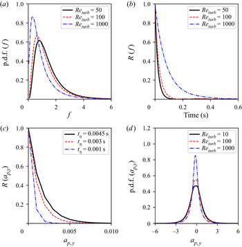
 $Re_{tur}$. In figure 2(a), the distribution of
 $f = \varepsilon ^{{2}/{3}}$ is shown for different Reynolds number:
 $Re_{tur}=50, 100, 1000$ and
 $\langle \varepsilon \rangle =100\,\textrm {m}^2\,\textrm {s}^{-3}$,
 $\tau _\eta =10^{-3}$ s. These distributions represent an averaged shape over the whole stochastic process. It is seen that with increasing the Reynolds number, the distributions become narrower and expose a long tail as the result of the particle response to events of the velocity ‘jumps’ in the fluid. Meanwhile the auto-correlation function of
 $f = \varepsilon ^{{2}/{3}}$ become more extended with increasing the Reynolds number. This is shown in figure 2(b). In agreement with experimental observations, mentioned in introduction, the acceleration has much narrower auto-correlation function than that for the acceleration norm. A heavy particle, interacting with energetic intertwined helical motion, preserves the magnitude of the acceleration longer than its direction. This is illustrated in figure 2(c), where the auto-correlation of
 $a'_{p,i=2}=({3}/{4})({\rho }/{\rho _p})\varepsilon ^{1/3}d_p^{-1/3} e_{p,i=2}$ is seen to be much narrower than in figure 2(b). By comparing this auto-correlation function at different Kolmogorov times
 $\tau _\eta = 0.001, 0.003, 0.0045$, with the same Reynolds number taken as
 $Re_{turb}=100$, i.e. preserving the turbulence intensity, but changing the mean dissipation rate
 $\langle \varepsilon \rangle$, it is seen that the auto-correlation function of the particle acceleration becomes narrower as the mean dissipation rate
 $\langle \varepsilon \rangle$ is increased. The reproduced intermittency effects are seen as well in figure 2(d), where the p.d.f.s of
 $a'_{p,i=2}$ at different Reynolds number
 $Re_{turb}=50,100,1000$ are shown. These effects are manifested in the form of extended tails of distribution, as the Reynolds number is increased.
(a) The p.d.f. of  $f=\varepsilon ^{{2}/{3}}$ for different
 $Re_{turb}= 10, 100, 1000$. (b) Auto-correlation function
 $R(f)$ for different
 $Re_{turb}= 10, 100, 1000$. (c) Auto-correlation function of
 $y$-component of stochastic particle acceleration i.e.
 $R(a_{p,y})$ for
 $Re_{turb}= 100$ but for different Kolmogorov time scales (
 $t_\eta$). (d) The p.d.f. of the
 $y$-component of stochastic particle acceleration i.e.
 $a'_{p,y}$ for different values of
 $Re_{turb}$.

3.3. Implementation of presented models in framework of LES
With expressions (3.4), (3.6) and (3.16), the motion equation of a particle depending on its size is given as follows. For droplets with  $d_p < \eta < \varDelta$, the droplet acceleration is given by
 \begin{equation} \frac{\textrm{d}u_{p,i}}{\textrm{d}t} = \frac{\tilde{u}_i- u_{p,i}}{\tau_p} + \sqrt{\frac{\varepsilon}{\tau_p}} e_{p,i}. \end{equation}
The subgrid droplets larger than the Kolmogorov scale have more inertia, and consequently, the spectral broadening associated with large-scale advection of structures on dissipative scales relative to these droplets is significant. Then for spray droplets with  $\eta < d_p < \varDelta$ (mainly in near-field spray), the second term in (3.4) may be stronger than the Stokes drag term. For such droplets, we assumed therefore zero-mean accelerations
 \begin{equation} \frac{\textrm{d}u_{p,i}}{\textrm{d}t} = \frac{3}{4}\frac{\rho}{\rho_p}\varepsilon^{1/3}d_p^{{-}1/3} e_{p,i}. \end{equation}
Along the particle path, the instantaneous viscous dissipation  $\varepsilon$ is simulated as log–normal stochastic process according to
 \begin{equation} \frac{\textrm{d}\varepsilon}{\varepsilon} ={-}\left[\textrm{ln}\frac{\varepsilon}{\varepsilon_\varDelta}- \frac{\sigma_\chi^2}{2} \right] T_{\chi}^{{-}1}\,\textrm{d}t + \sqrt{2 \sigma_\chi^2 T_{\chi}^{{-}1}}\,\textrm{d}W(t) \end{equation}
with the following parameters:
 \begin{equation} \varepsilon_{\varDelta}=C_l \frac{K_{sgs}^{3/2}}{\varDelta}; \quad T_\chi = \frac{\nu + \nu_{sgs} }{\varDelta^2};\quad \sigma_\chi^2 = {\rm ln} \left(\frac{\varDelta}{\eta}\right);\quad \eta = \left(\frac{\nu^3}{\varepsilon_\varDelta}\right)^{{1}/{4}}. \end{equation}
The expression for the variance in (3.23c) represents the influence of the local Reynolds number. This variance is calculated by typical size of the finite-difference cell, visited by a droplet at a given moment, and the local Kolmogorov length scale. The evolution of components of the direction  $e_{p,i}$, are simulated as diffusion process on a unit sphere according to (3.13) with
 $\tau _\eta = \sqrt {{\nu }/{\varepsilon _\varDelta }}$ as the correlation time scale. The random source due to aerodynamic drag in (2.8) is represented by the sum over all droplets in the given computational cell
 \begin{equation} S_{mom,i}^{stoch} ={-}\frac{1}{\varDelta^3}\sum_n \frac{\textrm{d}}{\textrm{d}t} (m_p u_{p,i})_n, \end{equation}
where  $m_p = \rho _p({{\rm \pi} d^3}/{6})$ is the mass of the
 $n$th droplet. The spray source term in (2.12) is usually expressed by summing the interactions between the sub-filtered fluid velocity
 $u'_i$ and the individual droplet
 \begin{equation} S_{p,sgs}^{stoch} ={-}\frac{1}{\varDelta^3}\sum_n \left(m_p \frac{d u_{p,i}}{dt} u'_i \right)_n, \end{equation}
where a model is needed for  $u'_i$. The latter is obtained in Bharadwaj, Rutland & Chang (Reference Bharadwaj, Rutland and Chang2009), Tsang et al. (Reference Tsang, Trujillo and Rutland2014) and Tsang et al. (Reference Tsang, Kuo, Trujillo and Rutland2019) by representing the unfiltered velocity in the form of an approximated deconvoluted velocity (Stolz, Adams & Kleiser Reference Stolz, Adams and Kleiser2001)
 \begin{equation} S_{p,sgs}^{stoch} ={-}\frac{1}{\varDelta^3}\sum_n \left[m_p \frac{\textrm{d} u_{p,i}}{\textrm{d}t} (2\tilde{u}_i - 3 \tilde{\tilde{u}}_i + \tilde{\tilde{\tilde{u}}}_i) \right]_n, \end{equation}
where tildes denote a repeated filtering procedure. The approximate deconvolution recovers flow scales of the order of the LES filter size. Therefore, the extension of this model is to complement  $u'_i = 2\tilde {u}_i - 3 \tilde {\tilde {u}}_i + \tilde {\tilde {\tilde {u}}}_i$ by the stochastic relative velocity seen by an individual droplet on SGS. Following § 3.2, for smaller droplets i.e.
 $d_p < \eta \ll \varDelta$ one can write
 \begin{equation} S_{p,sgs}^{stoch} ={-}\frac{1}{\varDelta^3}\sum_n \left[m_p \frac{\textrm{d} u_{p,i}}{\textrm{d}t} \left(2\tilde{u}_i - 3 \tilde{\tilde{u}}_i + \tilde{\tilde{\tilde{u}}}_i + \varepsilon^{{1}/{2}} \tau_p^{{1}/{2}} \right) \right]_n, \end{equation}
while for larger droplets, i.e.  $\eta < d_p < \varDelta$, assuming that the droplet response time includes most of turbulent times, the stochastic part can be expressed as
 \begin{equation} S_{p,sgs}^{stoch} ={-}\frac{1}{\varDelta^3}\sum_n \left[m_p \frac{\textrm{d} u_{p,i}}{\textrm{d}t} \left(2\tilde{u}_i - 3 \tilde{\tilde{u}}_i + \tilde{\tilde{\tilde{u}}}_i + \varepsilon^{{1}/{3}} d_p^{{1}/{3}} \right) \right]_n. \end{equation}
Here,  $\varepsilon$ is given by the stochastic process (3.22) along the droplet trajectory.
4. Stochastic mixing controlled evaporation model (SMICE)
Due to the non-stationary character of the flow, the droplet is never totally entrained by the gas; the surrounding conditions for this droplet are fluctuating, and consequently, its vaporization rate is also fluctuating. Another effect of turbulence is that the vaporization rate can be also altered by the presence of neighbouring droplets. The positions of these latter are controlled by turbulent structures in the flow. In this work we consider the quasi-stationary vaporization, i.e. the time of initial heating of the droplet and the time required to induce the radial motion in the gas at the droplet surface once the droplet recedes due to evaporation – both are negligible in comparison with turbulent times along the droplet path. The instantaneous vapour mass flux issued at the droplet surface is
 \begin{equation} F_{vs} ={-}\rho D_s \frac{(\boldsymbol{\nabla} Y_v)_s}{1-Y_{vs}}, \end{equation}
where  $Y_v$ is the vapour mass fraction,
 $Y_{vs}$ is its value at the droplets surface and
 $D_s$ is the vapour diffusivity in air. In the framework of classical assumptions of the droplet quasi-steady evaporation (see review of Jenny, Roekaerts & Beishuizen (Reference Jenny, Roekaerts and Beishuizen2012), for example), the gradient of the vapour mass fraction at the droplet surface is given by
 \begin{equation} (\boldsymbol{\nabla} Y_v)_s = \frac{Y_v^* - Y_{vs}}{d_p} {Pe}_p \frac{2}{e^{{Pe}_p}-1}, \end{equation}
where  $Y_v^*$, is the vapour mass fraction at a distance significantly larger that the droplet diameter
 $d_p$ and
 $Pe_p$ is the Péclet number of the evaporating droplet
 \begin{equation} {Pe}_p ={-}\frac{\rho_p}{\rho D_s}\frac{\textrm{d}}{\textrm{d}t}\left[ \frac{d_p^2}{8}\right] = \textrm{ln}(1 + B_Y).\end{equation}
Here,  $B_Y=(Y_{vs} - Y_v^*)/(1-Y_{vs})$ is the mass transfer number. Frossling's correlation (Faeth Reference Faeth1977), introduced usually into the expression (4.2), leads to
 \begin{equation} (\boldsymbol{\nabla} Y_v)_s = \frac{Y_v^* - Y_{vs}}{d_p} {Sh}_p, \end{equation}
where  ${Sh}_p$ is the Sherwood number. In our work, the Sherwood number is expressed in terms of the filtered flow variables, and is denoted as
 $\widetilde {Sh}_p$
 \begin{equation} \widetilde{Sh}_p = \left(2.0 + 0.6\widetilde{Re}_p^{1/2}Sc_p^{1/3}\right)\frac{\textrm{ln}(1+B_Y)}{B_Y}. \end{equation}
Here,  $\widetilde {Re}_p = |\boldsymbol {\tilde {u}} - \boldsymbol {u_p}|d_p/{\nu }$ is the filtered droplet Reynolds number and
 $Sc_p = {\nu }/{D}$ is the Schmidt number; if
 $B_Y\ll 1, \textrm {ln}(1+B_Y) \approx B_Y$. The vapour mass fraction
 $Y_v^*$ in surrounding of a point-wise droplet on residual scales is not completely known. Usually, it is attributed to the locally resolved filtered vapour mass fraction for the ensemble of all droplets which are located in a given computational cell. This implies that, inside the resolved eddies, the vapour leaving the droplet surface is immediately well stirred over the computational cell. Consequently, the source term in (2.4) and (2.5) is evaluated in LES solely in terms of filtered variables
 \begin{equation} \tilde{S}_{vap} = \frac{1}{\varDelta^3}\sum_n \left[\frac{{\rm \pi} d_p^2}{4} \tilde{F}_{vs} \right]_n, \end{equation}
where
 \begin{equation} \tilde{F}_{vs} = \bar{\rho} D_s \frac{Y_{vs} -\tilde{Y}_v}{d_p}\frac{1}{1 - Y_{vs}} \widetilde{Sh}_p. \end{equation}
The expression in brackets in (4.6) represents the vapour produced by the  $n$th evaporating droplet per unit time. The source term in the energy equation i.e. (2.5), has the following form:
 \begin{equation} \tilde{S}_{energy} = \frac{1}{\varDelta^3}\sum_n \left[ \frac{{\rm \pi} d_p^2}{4} \tilde{F}_{vs} \left( I_p + L_{vap} + \frac{1}{2}u_{p,i}u_{p,i} \right) + Q_p + m_p u_{p,i}\frac{\textrm{d} u_{p,i}}{\textrm{d}t} \right]_n, \end{equation}
where  $Q_p$ is the rate of heat conduction to the droplet surface per unit area,
 $I_p$ is the drop internal energy and
 $L_{vap}$ is the latent heat of vaporization; their sum is related to the vapour enthalpy (
 $h_{vap}$) and the equilibrium vapour pressure (
 $p_{vap}$), both calculated at the droplet temperature
 $T_p$, i.e.
 $I_p + L_{vap} = h_{vap}(T_p) - {p_{vap}(T_p)}/{\rho _p}$. More specific details on the governing equations of flow vaporizing sprays are given in many manuals (see for example Amsden et al. Reference Amsden, O'Rourke and Butler1989). In LES, the gradients of the vapour mass fraction and of the temperature in
 $Q_p$ on the droplet surface are determined by resolved fields.
In order to account for effects of sub-filter fluctuations on the vaporization rate, Bini & Jones (Reference Bini and Jones2009) proposed to complete the resolved Sherwood number in (4.7) by its stochastic part, as the random walk with the variance around the local magnitude of  $K_{sgs}^{{1}/{2}}$. The approach we propose hereafter is different from Bini & Jones (Reference Bini and Jones2009) model: it is based on the stochastic simulation of the gradient of the vapour mass fraction on the droplet surface, in which via the stochastic process, the physical time scale of the auto-correlation is introduced, and the main focus is put on effects of small-scale intermittency in the evaporation of droplets. Namely, along the droplet trajectory, we simulate the random function
 $Y_v^{stoch}$ which is varying within the interval between the vapour mass fraction
 $\widetilde {Y_v}$, resolved on the coarse LES mesh, and its value at the droplet surface
 $Y_{vs}$, i.e.
 $Y_v^{stoch}\in [\tilde {Y}_v, Y_{vs}]$, and correspondingly
 \begin{equation} (\boldsymbol{\nabla} Y_v)^{stoch}_s = \frac{Y_v^{stoch} - Y_{vs}}{d_p} \widetilde{Sh}_p. \end{equation}
Thereby, the stochastic source terms in (2.9)–(2.11) have the following form:
 \begin{equation} {S}_{vap}^{stoch} = \frac{1}{\varDelta^3}\sum_n \left[\frac{{\rm \pi} d_p^2}{4} {F}_{vs}^{stoch} \right]_n, \end{equation}
where
 \begin{gather} {F}_{vs}^{stoch} = \bar{\rho} D_s \frac{Y_{vs} -{Y}_v^{stoch}}{d_p}\frac{1}{1 - Y_{vs}} \widetilde{Sh}_p, \end{gather}
 \begin{gather} {S}_{energy}^{stoch} = \frac{1}{\varDelta^3}\sum_n \left[ \frac{{\rm \pi} d_p^2}{4} {F}_{vs}^{stoch} \left( I_p + L_{vap} + \frac{1}{2}u_{p,i}u_{p,i} \right) + Q_p + m_p u_{p,i}\frac{\textrm{d} u_{p,i}}{\textrm{d}t} \right]_n. \end{gather}
It is seen that, different from the standard evaporation model, i.e.  $d^2$-law, the expression (4.11) contains the random multiplier
 $(Y_{vs} - {Y}_v^{stoch})/(Y_{vs} - \tilde {Y}_v)\in [0, 1]$. The idea behind the stochastic model for
 ${Y}_v^{stoch}$ follows the partially stirred reactor model, which was proposed to account for the turbulence–chemistry interaction (Vulis Reference Vulis1961; Chomiak & Karlsson Reference Chomiak and Karlsson1996; Sabelnikov & Fureby Reference Sabelnikov and Fureby2013). In the Vulis model, the chemical reaction and turbulent mixing are considered as the succession of two steady-state sub-processes, and thereby the chemical reaction rate, evaluated at a certain intermediate concentration, and the intensity of turbulent mixing, conditioned on that concentration, represent two mutually controlling factors. By same analogy, we assume that the global evaporation process consists of the succession of two steady-state sub-processes, evaporation and mixing. The latter is due essentially to the intermittent regions of turbulent fine structures which occupy a small fraction of the flow within the considered volume. The main suggestion is that the evaporation rate is strongly enhanced once the droplet is visiting these regions, and their volume fraction is to be proportional to the time scale fraction
 $\tau _{mix}/(\tau _{mix} + \tau _{vap})$, where
 $\tau _{mix}$ is the mixing time scale and
 $\tau _{vap}$ is the vaporization time scale. The smaller the mixing time (
 $\tau _{mix}$), the thinner are the fine turbulent structures and the thinner are the stretched zones of effective evaporation and, thereby, a more intensive mixing process is induced. If this fraction tends to zero,
 $\tau _{mix}/(\tau _{mix} + \tau _{vap}) \approx 0$, i.e.
 $\tau _{mix} \ll \tau _{evap}$, the mixing is intensive, and the global evaporation process corresponds to well-stirred conditions
 $Y_v^{stoch} \approx \tilde {Y}_v$. In contrast, if the ambient around a droplet is non-turbulent,
 $\tau _{mix} \gg \tau _{evap}$ and
 $\tau _{vap}/(\tau _{mix} + \tau _{vap}) \approx 0$ (as in a cluster of droplets, for example), the dilution of the droplet environment by surrounding air, which is of a diffusive nature, is much less effective. In the limit of zero gradient of the vapour mass fraction on the droplet surface,
 $Y_v^{stoch} \approx Y_{vs}$, there is no evaporation. To satisfy these conditions, we state the following expression:
 \begin{equation} Y_v^{stoch} = \tilde{Y}_v \frac{\tau_{vap}}{\tau_{vap} + \tau_{mix}} + Y_{vs} \frac{\tau_{mix}}{\tau_{vap} + \tau_{mix}}, \end{equation}
equivalently to the equality of both intensities, of evaporation and of mixing
 \begin{equation} \frac{Y_{vs} - Y_v^{stoch}}{{Y_v^{stoch} - \tilde{Y}_{v}}} = \frac{\tau_{vap}}{\tau_{mix}}. \end{equation}
With (4.13), the expression (4.9) can be rewritten as
 \begin{equation} (\boldsymbol{\nabla} Y_v)^{stoch}_s = \frac{b}{b+1}\frac{\tilde{Y}_v - Y_{vs}}{d_p} \widetilde{Sh}_p, \end{equation}
where  $b={\tau _{vap}}/{\tau _{mix}}$, represents the vaporization Damkhöler number. Here,
 $\tau _{mix}$ may be taken as the instantaneous Kolmogorov time i.e.
 $\tau _{mix} = \sqrt {{\nu }/{\varepsilon }}$, where
 $\varepsilon$ is governed along the droplet trajectory by the stochastic log–normal process. In this way the intermittency effects are introduced in the droplet evaporation model. Along with the log–normal process (3.7), presuming
 $\langle \varepsilon \rangle$,
 $\nu$,
 $Re_{turb}$, the stochastic properties of the coefficient
 $\frac {b}{b+1}$ are shown in figure 3. With the same turbulent Reynolds number,
 $Re_{turb}=100$, and varying
 $\langle \varepsilon \rangle$, figure 3(a) illustrates the influence of the intensity of fine structures
 $(\tau _\eta = \sqrt {{\nu }/({\langle \varepsilon \rangle }}))$ on the mean value
 $\langle {b}/({b+1}) \rangle$ in (4.15). It is seen that, with higher
 $\langle \varepsilon \rangle$, the mean estimate of the vapour mass fraction gradient on the droplet surface in (4.15) is increased. Figure 3(b) shows the effect of the turbulent Reynolds number,
 $Re_{turb}$, on the root-mean square of
 ${b}/({b+1})$, for the same
 $\langle \varepsilon \rangle = 100\,\textrm {m}^2\,\textrm {s}^{-3}$. It is seen that the higher the Reynolds number is the higher is the variance of
 ${b}/({b+1})$ in (4.15), i.e. there is more fluctuation in the vaporization rate in response to the irregular local flow structure. There are different possible definitions of the vaporization time scale
 $\tau _{vap}$. In this work, using the Frössling correlation, we adapted the expression of the vapour mass flow leaving the droplet surface per unit time and per unit mass of the gaseous mixture in the considered computational cell
 \begin{equation} {-}\frac{\textrm{d}m_p}{\textrm{d}t}\frac{1}{{\varDelta^3}\bar{\rho}}=\frac{{Y_{vs} -\tilde{Y}_v}}{\tau_{vap}};\quad \tau_{vap}^{{-}1} = {\rm \pi}D_s d_p \frac{1}{1-Y_{v,s}} \widetilde{Sh}_p \frac{1}{\varDelta^3}. \end{equation}
At the end of this section, note also that the Frössling correlation in the Sherwood number (4.5) was established for  $10 < Re_p < 1800$ (see Faeth (Reference Faeth1977), and references therein for higher Reynolds numbers). Since the vaporizing subgrid droplets larger than the Kolmogorov scale may be surrounded by turbulent shear layers, the application of the Frössling correlation, based on the instantaneous relative velocity of the droplet, is an open question (see discussions in Birouk & Gökalp (Reference Birouk and Gökalp2002). In our simulations, the expression (4.5) was retained in terms of filtered parameters
 $\widetilde {Sh}_p$ for droplets smaller and larger than the Kolmogorov length scale. The local filtered Reynolds number is usually
 $\widetilde {Re}_p < 1000$. The assumption behind expression (4.9) is that the contribution of the subgrid turbulence comes from
 $({Y_{v}^{stoch} - Y_{vs}})/{d_p}$, while
 $\widetilde {Sh}_p$ is slowly varying. On the other hand, it is clear that the presence of boundary layers in the vicinity of droplets with
 $d_p > \eta$ does not contradict the main assumption (4.14): the intensity of the vapour release from a droplet is equal to the intensity of its turbulent mixing, and the latter is controlled by inhomogeneous structures on SGS. The above described stochastic evaporation model, is applied and assessed in the following sections.
(a) Mean of  ${b}/({b+1})$ for different values of dissipation rate
 $\langle \varepsilon \rangle$ for same
 $Re_{turb}=100$. (b) Variance of
 ${b}/({b+1})$ corresponding to different values of variance for same
 $\langle \varepsilon \rangle = 100\,\textrm {m}^2\,\textrm {s}^{-3}$.

5. Model assessment and further discussion
Two different experimental set-ups are used in this study to characterize the performance of the new stochastic models for droplet dispersion and evaporation given by (3.20)–(3.28) with (4.10)–(4.13). The first set of experiments from an engine combustion network (ECN), provide quantitative measurements of fuel–air mixing characteristics in high-pressure liquid spray injection with conditions reflective of diesel engines. In these experiments, the liquid fuel is injected into the gas chamber at super-critical conditions. This may raise questions about the existence of droplets (Bellan Reference Bellan2000; Selle & Ribert Reference Selle and Ribert2008), which is the intrinsic assumption of the models in §§ 3 and 4. To the best of our current knowledge, the recent experimental observations confirm the physical validity of such an assumption – the liquid/gas interface in the mixture persists at super-critical conditions of the chamber, and gives rise to a spray-like dynamics and evaporation (Jofre & Urzay Reference Jofre and Urzay2021). The clear evidence from the highly resolved optical imaging in Crua, Manin & Pickett (Reference Crua, Manin and Pickett2017) is that the surface tension and droplet production are significant in the conditions of ECN sprays. Although these conditions are above the critical point of the n-dodecane, the initial temperature of the fuel is sub-critical, and finite time is needed for the heat transfer to bring the fuel to its super-critical value. The measurements in Crua et al. (Reference Crua, Manin and Pickett2017) show that the evaporation of n-dodecane droplets in ECN sprays is faster than the time required to reach the super-critical conditions. In the same operating conditions, the existence of a liquid/gas interface, albeit weakening because cellular structures appear, is also recognized from the ballistic imaging in Falgout et al. (Reference Falgout, Rahm, Sedarsky and Linne2016). On top of this, even if super-critical conditions have been attained in the chamber for both fuel and air, the recent analysis of the thermodynamics and transport processes in the multi-component systems in Jofre & Urzay (Reference Jofre and Urzay2021) suggest that liquid-like and gas-like streams, being brought into contact, will tend to be separated by persisting interfaces subject to surface-tension forces. The second experiment concerns turbulent spray evaporation in a simplified co-axially flowing gas combustor configuration. Also a relative comparison of the different flow statistics for the aforementioned test cases with two other state-of-the-art models i.e. the Wang & Squires (Reference Wang and Squires1996) dispersion model with classical  $d^2$-law evaporation model and the more recently proposed stochastic models of Bini & Jones (Reference Bini and Jones2008, Reference Bini and Jones2009) described in § 3.1, is also presented. This is followed by a short discussion on the numerical simulations.
5.1. Non-reacting and non-evaporating diesel-like sprays
The open-source database of ECN spray experiments (Idicheria & Pickett Reference Idicheria and Pickett2007; Pickett et al. Reference Pickett, Genzale, Bruneaux, Malbec, Hermant, Christiansen and Schramm2010, Reference Pickett, Manin, Genzale, Siebers, Musculus and Idicheria2011; Payri et al. Reference Payri, Viera, Wang and Malbec2016; Kastengren et al. Reference Kastengren, Ilavsky, Viera, Payri, Duke, Swantek, Tilocco, Sovis and Powell2017) provides detailed measurements of different quantities like temporal evolution of the liquid spray-tip and vapour penetration lengths, spatial distribution of gas-phase velocities and fuel–air mixture fraction. The typical experimental set-up referred to as Spray-A consists of a liquid n-dodecane jet issued from a nozzle with a diameter of  $90\,\mathrm {\mu }\textrm {m}$ into a pre-heated constant volume gas chamber. The temperature and pressure of the chamber are varied accordingly in order to always maintain the ambient gas density at a constant value of
 $22.8\,{\textrm {kg}}\,{\textrm {m}^{-3}}$. In order to evaluate the effect of the droplet dispersion models on spray structure, two different low-temperature spray experiments with injection pressures of 150 and 50 MPa are considered. For these experiments the ambient gas temperature and pressure are maintained at 440 K and 2 MPa respectively. The evaporation rates for these test cases are considered to be negligibly small. The ambient gas for these test cases is composed of pure
 $N_2$ gas. The liquid velocity and the Reynolds number based on the jet exit conditions for the two test cases are of the order of
 $300 - 600\,\textrm {m}\,\textrm {s}^{-1}$ and
 $1 \times 10^4 - 10^5$, respectively. The specifics of the different non-evaporating experimental conditions are provided in table 1. The constant volume spray chamber is represented by a cylindrical domain of length 100 mm with a diameter of 50 mm in the computations. The computational domain is discretized into hexahedral cells with a uniform grid size of 0.25 mm in both axial and radial directions. This mesh resolution is referred to as the coarse grid or C-Grid. Another finer mesh referred to as the F-Grid with a cell size linearly varying from 0.125 to 0.25 mm both in axial and radial directions is used to study the effects of grid resolution. In the framework of the LES approach, in which filtering is equivalent to spatially weighted averaging, the parcels are formed from a distribution of drop sizes, velocities and temperatures within the volume of filtering, and then the evolution of these parcels is simulated by a discrete-particle technique. This study is based on the classical ‘blob’ approach of Amsden et al. (Reference Amsden, O'Rourke and Butler1989), wherein the initial size of all the parcels injected is assumed to be the same as the nozzle diameter. The fragmentation of droplets is then modelled using the well-known breakup model of Beale & Reitz (Reference Beale and Reitz1999), wherein the breakup is characterized by relaxation to typical size estimates of the fastest growing instabilities on the droplet surface. While the Kelvin–Helmholtz (KH) instability is applied for representing the continuous stripping of the mass from initial ‘blobs’ in the near-nozzle region, the Rayleigh–Taylor (RT) instability mechanism is used as a model for the secondary breakup of droplets. This approach is usually referred to as the KH–RT model and is implemented in the majority of spray combustion solvers. The model constants for the KH–RT breakup model used in this study are same as those found in Wehrfritz et al. (Reference Wehrfritz, Vuorinen, Kaario and Larmi2013). The droplet collisions and coalescence are not considered in this study. OpenFOAM, which is widely used in simulations of turbulent multi-phase flows, is applied also in this work. The Eulerian gaseous flow is solved using a low Mach number variable density flow solver based on the pressure-implicit with splitting of operators (PISO) algorithm. For discretization of spatial gradients second-order numerical schemes are used, an implicit first-order Euler scheme is used for the time integration. Liquid spray penetration length is an important parameter characterizing the overall spray dispersion. At any given instance of time, it is defined as the axial distance where the accumulated liquid droplet mass reaches
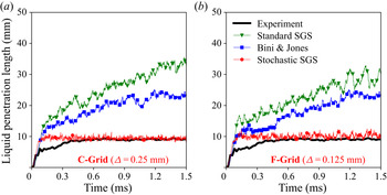
 $95\,\%$ of the total liquid mass injected. First, in order to evaluate the significance of the spray source/sink term in the TKE equation, a comparison of the evolution of spray-tip penetration lengths predicted by different dispersion models on the coarse grid resolution of
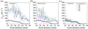
 $\varDelta = 0.25\,\textrm {mm}$ is shown in figure 4. From the relative comparisons, it can be seen that in the considered case of the high-speed ECN sprays, the rate at which turbulent subgrid eddies are doing work in dispersing the spray droplets makes very little contribution to the spray-tip evolution. Probably this is a reason why, in a number of ECN spray simulations (see for example, Kaario et al. Reference Kaario, Vuorinen, Hulkkonen, Keskinen, Nuutinen, Larmi and Tanner2013; Senecal et al. Reference Senecal, Mitra, Pomraning, Xue, Som, Banerjee, Hu, Liu, Rajamohan and Deur2014), this term is neglected. Next, the distributions of time-averaged SGS kinetic energy and the mean gas-phase velocities along the spray centreline predicted by the different models are shown in figures 5 and 6 to qualitatively illustrate the contribution of the spray source term in the subgrid TKE equation. The time averaging is performed over a period of 1.0 ms (i.e. from 0.5 to 1.5 ms). From the results, it can be seen that the average gas velocity and SGS kinetic energy predicted by the stochastic drag model is almost half of the values predicted using the Wang & Squires (Reference Wang and Squires1996) and Bini & Jones (Reference Bini and Jones2008). The results also show that the relative influence of the source term on both the gas velocity and SGS kinetic energy is minor for all the dispersion models. Therefore, for further comparisons, the results corresponding to ECN spray simulations without the spray source term in the subgrid TKE equation are presented. In order to evaluate the grid sensitivity of the dispersion models, a comparison of the spray-tip evolution for two different grid resolutions with the experimental data for the high-pressure injection case of NEV-A1 is shown in figure 7. In comparison with the experiment, the faster spray-tip penetration predicted by both Wang & Squires (Reference Wang and Squires1996) and Bini & Jones (Reference Bini and Jones2008) models even on finer grid resolution of
 $\varDelta =0.125\,\textrm {mm}$, reflects underestimation of the droplet dispersion by these models. On the other hand, the stochastic drag (SD) model is seen to be more efficient in predicting the spray evolution even on coarse grid resolution of
 $\varDelta =0.25\,\textrm {mm}$. In the case of the SD model, it can also be seen that the penetration length evolution is less sensitive to the grid resolution compared with the standard dispersion models. Applying the same KH–RT breakup model, it is interesting to study the influence of the dispersion model on the resulting droplet sizes from spray breakup. To this end, a comparison of the spatial evolution of the Sauter mean diameter (SMD) of droplets along the spray axis as predicted by different models with the experiment at a time
 $t=1.5\,\textrm {ms}$ after start of injection (ASOI) on a grid resolution of
 $\varDelta =0.125\,\textrm {mm}$ is shown in figure 8. The results indicate that both the Wang & Squires (Reference Wang and Squires1996) and Bini & Jones (Reference Bini and Jones2008) dispersion models give a slower breakup rate with larger SMD values compared with the experiment, even at the finer grid resolution of
 $\varDelta =0.125\,\textrm {mm}$. Also with these two models, the droplet sizes resulting from spray breakup (indicated by SMD values far away from the nozzle exit i.e.
 ${\approx }5\,\mathrm {\mu }\textrm {m}$) are much larger than the experimental values. On the other hand, the use of SD model induces relatively faster breakup rate with resulting droplet sizes much closer to the measured SMD values (
 ${\approx }1\,\mathrm {\mu }\textrm {m}$). Again, it can be observed that the droplet size statistics resulting from the SD model are less sensitive to grid resolution, while the other two models produce relatively faster breakup of droplets with smaller sizes on finer grid resolution.
Comparison of temporal evolution of spray-tip penetration length predicted with (red) and without (blue) the spray source/sink term in the subgrid TKE equation by Wang & Squires (Reference Wang and Squires1996) (green), Bini & Jones (Reference Bini and Jones2008) (blue), stochastic drag (SD) (red) models with the NEV-A1 experiment (black) for the grid resolution of  $\varDelta =0.25\,\textrm {mm}$.

Comparison of time-averaged SGS kinetic energy predicted with (Red) and without (Blue) spray-induced turbulence source term by Wang & Squires (Reference Wang and Squires1996), Bini & Jones (Reference Bini and Jones2008), SD (Red) models for the grid resolution of  $\varDelta =0.25\,\textrm {mm}$.

Comparison of time-averaged gas-phase velocity predicted with (Red) and without (Blue) spray-induced turbulence source term by Wang & Squires (Reference Wang and Squires1996), Bini & Jones (Reference Bini and Jones2008), SD (Red) models for the grid resolution of  $\varDelta =0.25\,\textrm {mm}$.

Comparison of temporal evolution of spray-tip penetration length predicted by Wang & Squires (Reference Wang and Squires1996) (Green), Bini & Jones (Reference Bini and Jones2008) (blue), SD (Red) models with the NEV-A1 experiment (black) for two grid resolutions of  $\varDelta =0.25\,\textrm {mm}$ (a) and
 $\varDelta =0.125\,\textrm {mm}$ (b).

Comparison of SMD of droplets predicted by Wang & Squires (Reference Wang and Squires1996) (Green), Bini & Jones (Reference Bini and Jones2008) (blue) and SD (Red) model along the spray centreline at time = 1.5 ms after start of ignition (ASOI) for two grid resolutions of  $\varDelta =0.25\,\textrm {mm}$ (a) and
 $\varDelta =0.125\,\textrm {mm}$ (b).

Experimental conditions of non-evaporating ECN Spray-A test cases

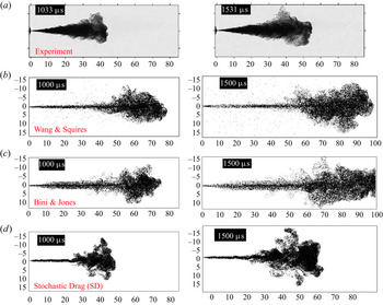
In order to qualitatively illustrate the mentioned differences in the spray configuration predicted by different dispersion models, a comparison of the instantaneous images with the experiment for time instances of 1.0 ms and 1.5 ms after start of injection (ASOI) is provided in figure 9. The computations correspond to the grid resolution of  $\varDelta = 0.25\,\textrm {mm}$. While the spray structure predicted by the SD model remains similar to the Schlieren images of the experiment, the other two models predict a spray structure with an excessively penetrative liquid core. Moreover in case of Wang & Squires (Reference Wang and Squires1996), the spray core is surrounded by large number of very small droplets radially dispersed.
Comparison of instantaneous spray structures at times  $t =1.0\,\textrm {ms}$ and 1.5 ms ASOI predicted by Wang & Squires (Reference Wang and Squires1996), Bini & Jones (Reference Bini and Jones2008) and SD models on a grid resolution of
 $\varDelta =0.25\,\textrm {mm}$ with the experimental Schlierien images.

At lower injection pressures, as in the case of NEV-A2, the experiments have shown that spray breakup ends within the first few millimetres of injection and the spray structure is controlled only by turbulent dispersion. So, next a comparison of the temporal evolution of liquid spray-tip penetration predicted by different models for two different grid resolution for the NEV-A2 test case are shown in figure 10. From the results, it can again be seen that, while the SD model accurately predicts the spray evolution even on a coarser grid resolution, the standard dispersion models tend to over-predict the penetration lengths even on the finer grid resolution. In general, the simulation in high-pressure ECN spray conditions lends substantial support to properties of the SD model, introduced in § 3. Being designed to characterize the interaction solely with strong turbulent motions on smallest unresolved scales, and providing the long spatial correlation for the particle stochastic acceleration, the SD model shows a weak sensitivity to the grid resolution, and the predictions by this model are quite closely to experimental observations. At the same time, the droplet dispersion models, based on the stochastic estimate of the sub-filter fluid velocity, over-predict the spray penetration lengths and display an acute sensitivity to the grid resolutions.
Comparison of temporal evolution of spray-tip penetration length predicted by Wang & Squires (Reference Wang and Squires1996) (Green), Bini & Jones (Reference Bini and Jones2008) (blue), SD (Red) models with the NEV-A2 experiment (black) for two grid resolutions of  $\varDelta =0.25\,\textrm {mm}$ (a) and
 $\varDelta =0.125\,\textrm {mm}$ (b).

5.2. Non-reacting and evaporating diesel-like sprays
In order to characterize the influence of stochastic SGS evaporation models, two different evaporating spray experiments from the ECN database were considered in this study. The first test case is the Spray-A experiment. Here, n-dodecane is injected at a pressure of 150 MPa into a pre-heated gas with an ambient temperature of 900 K and density of  $22.8\,{\textrm {kg}}\,{\textrm {m}^{-3}}$. The Spray-A experiment provides statistics of gas-phase velocity and vapour mass fraction. In addition to the quantitative comparisons of different statistics provided by Spray-A, the Spray-H test case is used to qualitatively compare the instantaneous spray jet structure at different time instances. In case of Spray-H, a liquid jet of n-heptane is issued from a nozzle diameter of 100
 $\mathrm {\mu }$m with an injection pressure of 150 MPa into an ambient gas at a temperature of 1000 K and a density of
 $14.2\,{\textrm {kg}}\,{\textrm {m}^{-3}}$. The specific details of the experimental conditions are presented in table 2. Unlike isothermal sprays, in the case of evaporating sprays the liquid spray-tip penetration length attains a steady-state value, where the total evaporation rate is equal to the fuel injection rate, thereby quantifying the overall evaporation rate. On the other hand, the vapour penetration length progresses with time, quantifying the overall dispersion and fuel–air mixing rate. In figures 11 and 12 the numerical positions of both tips predicted by the different modelling approaches are compared with the measurements of Spray-A. The numerical values of both the liquid and vapour tip penetration are compared for two different grid sizes,
 $\varDelta =0.25\,\textrm {mm}$ and
 $\varDelta =0.125\,\textrm {mm}$. It is clearly seen that, on a given mesh, the new stochastic models for vaporizing droplets predict better both the global dispersion and vaporization parameters compared with the stochastic models of Bini & Jones (Reference Bini and Jones2008, Reference Bini and Jones2009) and the standard approach (the Wang & Squires (Reference Wang and Squires1996) model for dispersion with the classical
 $d^2$-law evaporation model). As in the case of isothermal sprays, the new stochastic SGS model of vaporizing droplets exhibit much less sensitivity to the mesh spacing than in the case of the other two modelling approaches. Since each repetition of the experiment represents a single realization of the spray, 30–40 realizations of the same experiment are performed to obtain ensemble-averaged statistics for the local gas-phase flow parameters like the velocity and vapour mass fraction. In order to emulate the same numerically, random seeding procedure (Senecal et al. Reference Senecal, Mitra, Pomraning, Xue, Som, Banerjee, Hu, Liu, Rajamohan and Deur2014; Hu et al. Reference Hu, Banerjee, Liu, Rajamohan, Deur, Xue, Som, Senecal and Pomraning2015; Pei et al. Reference Pei, Som, Pomraning, Senecal, Skeen, Manin and Pickett2015; Ameen, Pei & Som Reference Ameen, Pei and Som2016) is adopted in this study. The random seeding approach generates a different sequence of random numbers used for modelling different spray sub-processes like injection, dispersion and evaporation, thereby producing different realizations of both Lagrangian and Eulerian flow statistics for the same initial and boundary conditions. For each modelling approach, 10 different realizations of LES are simulated in order to obtain the ensemble-average statistics. Figure 13 provides a comparison of 5 different realizations of vapour mass fraction profiles generated along the spray centreline for the three different modelling approaches. The mean and variance of local gas flow velocity and vapour mass fraction fields are obtained by averaging over ten different realizations for each modelling approach. First, a quantitative comparison of the mean gas-phase velocities and vapour mass fraction evolution along the spray centreline are given for time
 $t=1.5\,\textrm {ms}$ ASOI for two different grid resolutions (
 $\varDelta =0.25\,\textrm {mm}, 0.125\,\textrm {mm}$) in figures 14 and 15. Next, a comparison of the spatial distributions of the mean and variance of local vapour mass fraction and gas-phase velocities at three different longitudinal positions
 $(20\,\textrm {mm}, 30\,\textrm {mm}, 40\,\textrm {mm})$ for time
 $t=1.5\,\textrm {ms}$ ASOI on a grid resolution of
 $\varDelta =0.125\,\textrm {mm}$ are shown in figures 16 and 17. While the spatial distribution of vapour mass fraction quantifies the local vaporization rate, the velocity distributions quantify the momentum transfer from the liquid droplets and the air entrainment process. It is seen that, different from other models, the application of SD and SMICE models leads to a reasonably accurate prediction of both the first- and second-order statistics of both the vapour mass fraction and gas velocity even at coarser grid resolutions. The spatial distribution of the variance of both the vapour mass fraction and gas-phase velocities for the stochastic models still do not exactly match with the experimental distributions as the number of realizations used for averaging is still significantly lower than that used in the experiments. Finally a comparison of the instantaneous spray structure predicted by a single realization of different modelling approaches at four different time instances of spray evolution for the Spray-H test case are shown in figure 18. While the new stochastic models for vaporizing droplets give an accurate description of both the vapour penetration and also the spatial distribution of vapour mass fraction, the other two modelling approaches show much faster penetration of vapour with a lower intensity of the vapour mass fraction.
Experimental conditions of evaporating ECN Spray-A and Spray-H test cases

Comparison of liquid spray-tip evolution predicted by standard SGS (Green) i.e. Wang & Squires (Reference Wang and Squires1996) dispersion model with classical  $d^2$-law evaporation model, stochastic models of Bini & Jones (Reference Bini and Jones2008, Reference Bini and Jones2009) (blue), stochastic SGS: SD model and SMICE model (red), with the ECN-A experiment (black) for two grid resolutions of
 $\varDelta =0.25\,\textrm {mm}$ (a) and
 $\varDelta =0.125\,\textrm {mm}$ (b).

Comparison of vapour penetration length evolution predicted by standard SGS (Green) i.e. Wang & Squires (Reference Wang and Squires1996) dispersion model with classical  $d^2$-law evaporation model, stochastic models of Bini & Jones (Reference Bini and Jones2008, Reference Bini and Jones2009) (blue), stochastic SGS: SD model and SMICE model (red), with the ECN-A experiment (black) for two grid resolutions of
 $\varDelta =0.25\,\textrm {mm}$ (a) and
 $\varDelta =0.125\,\textrm {mm}$ (b).

Multiple realizations of gas-phase velocities along the spray centreline generated using the random seeding approach. (a) the Wang & Squires (Reference Wang and Squires1996) model with  $d^2$ law (standard SGS); (b) stochastic models of Bini & Jones (Reference Bini and Jones2008, Reference Bini and Jones2009); (c) SD with SMICE (stochastic SGS) for the grid resolution of
 $\varDelta =0.125\,\textrm {mm}$.

Mean gas-phase velocity along spray axis at a location 0.64 mm offset from the centreline at time  $t=1.5\,\textrm {ms}$ ASOI. Comparison for two different grid resolutions of
 $\varDelta =0.25\,\textrm {mm}$ (red),
 $\varDelta =0.125\,\textrm {mm}$ (blue) with ECN-A data (black circles). (a) the Wang & Squires (Reference Wang and Squires1996) model with
 $d^2$ law (standard SGS); (b) stochastic models of Bini & Jones (Reference Bini and Jones2008, Reference Bini and Jones2009); (c) SD with SMICE (stochastic SGS).

Mean vapour mass fraction along spray axis at a location 0.64 mm offset from centreline at time  $t=1.5\,\textrm {ms}$ ASOI. Comparison for two different grid resolutions of
 $\varDelta =0.25\,\textrm {mm}$ (red),
 $\varDelta =0.125\,\textrm {mm}$ (blue) with ECN-A data (black circles). (a) the Wang & Squires (Reference Wang and Squires1996) model with
 $d^2$ law (standard SGS); (b) stochastic models of Bini & Jones (Reference Bini and Jones2008, Reference Bini and Jones2009); (c) SD with SMICE (stochastic SGS).

Radial distributions of mean and variance of vapour mass fraction at axial locations of 20 mm, 30 and 40 mm; at time  $t=1.5\,\textrm {ms}$ ASOI and
 $\varDelta =0.125\,\textrm {mm}$; experiment: ECN-A data; standard SGS (Green): the Wang & Squires (Reference Wang and Squires1996) model with
 $d^2$-law; Bini & Jones (Reference Bini and Jones2008, Reference Bini and Jones2009) stochastic models (Blue); stochastic SGS (Red): SD with SMICE.

Radial distributions of mean and variance of axial gas-phase velocities at axial locations of 20 mm, 30 and 40 mm; at time  $t=1.5\,\textrm {ms}$ ASOI and
 $\varDelta =0.125\,\textrm {mm}$; experiment: ECN-A data; standard SGS (Green): the Wang & Squires (Reference Wang and Squires1996) model with
 $d^2$-law; Bini & Jones (Reference Bini and Jones2008, Reference Bini and Jones2009) stochastic models (Blue); stochastic SGS (Red): SD with SMICE.

Comparison of spray images for a grid resolution of  $\varDelta =0.125\,\textrm {mm}$ at times 0.49 ms, 0.68 ms, 0.9 ms and 1.1 ms ASOI with snapshots from experiment: ECN-H data; stochastic SGS: SD with SMICE; standard SGS: the Wang & Squires (Reference Wang and Squires1996) model with
 $d^2$-law; Bini & Jones (Reference Bini and Jones2008) stochastic models.

5.3. Turbulent spray evaporation in a co-flowing gas combustor
The third test case used for the assessment of the stochastic models for vaporizing droplets is the co-axial spray combustor experiment from Sommerfeld & Qiu (Reference Sommerfeld and Qiu1998). A schematic of the experimental set-up shown in figure 19 is reproduced in the simulation. An iso-propyl alcohol spray is injected from a hollow cone spray atomizer with a diameter of 20 mm into a pre-heated turbulent co-flow of air issuing from an annular injection tube with an inner diameter of 40 mm and an outer diameter of 64 mm. The mass flow rates of the air and of the liquid spray are 28.3 and 0.44  $\textrm {g}\,\textrm {s}^{-1}$ respectively. The hot air is issued at 18
 $\textrm {m}\,\textrm {s}^{-1}$ and at a temperature of 373 K while the liquid is injected at a temperature of 313 K. Taking the annular radius of the co-flow as a reference length scale, the bulk flow Reynolds number for the flow can be approximated to be around
 $2\times 10^4$. The detailed measurements are provided close to the nozzle exit as a set of initial conditions for the droplet size distribution, as well as for the correlations between size, location and velocity of the droplet. So, in the simulation there is no need to simulate the breakup of droplets.
Schematic representation of co-axial flow combustor experiment (a) and the corresponding computational geometry used for simulations (b).

In order to reduce the computational effort, the turbulent fluctuations at the exit of the annular pipe are generated from a priori periodic flow simulation. The inflow data are generated and stored over five flow through times, for every few computational time steps of the channel flow simulation. The velocity profiles are then mapped onto the gas flow inlet located 50 mm above the atomizer. The velocity profiles are linearly interpolated for time steps between any two consecutive time intervals of mapping. Since only a finite sized domain is used instead of simulating the entire test section, a convective boundary condition is applied at the outlet in order to ensure conservation of mass flow leaving the domain. No-slip and adiabatic boundary conditions are used for velocity and temperature at the walls. The O-grid technique is used to generate a structured hexahedral mesh with increasing grid density in the spray injection and annular gas flow regions. The grid size is varying from 0.25 mm in the regions closer to the spray atomizer to 2.5 mm in the outer wall regions both in the axial and radial directions. The droplets are injected from a plane 3 mm downstream of the atomizer where the measurements of the spray size and velocity correlations are available. The position of each droplet is randomly sampled over a radial distance of 10 mm around the centre. The droplet size distributions are experimentally measured over 10 discrete radial zones each with a size of 1 mm. Depending on the droplet position, the droplet diameter is sampled from the size distribution corresponding to the radial zone containing the droplet. Then the velocity of the droplet is calculated based on the measured velocity–size correlations. The axial and radial velocity components of the droplet determine the angle at which it is injected into the considered domain.
Also depending on the time step value, the number of droplets injected is approximated to match the liquid mass flow rate. Figure 20 shows the radial profiles of the mean and r.m.s. of axial velocity fields for droplets at different longitudinal cross-sections from 25 to 400 mm. These profiles are obtained by ensemble averaging over all droplet sizes and for 250 samples of discrete time intervals spread over two flow through times. It is seen that except for the profile of r.m.s. fluctuations at 50 mm, the statistical distributions of the axial velocity of droplets are predicted relatively well. The injected droplets are entrained by the high-speed co-flow, reproducing the velocity profiles similar to the jet flow; droplets then move downstream and spread radially outwards. Thereby negative velocities of droplets are a result of the generated re-circulation zones in the gas flow. Next, an assessment of the mean and r.m.s. of the droplet diameter at different axial locations is shown in figure 21. In the continuous hollow cone spray, the smaller droplets are dragged into the core by the entrained air, whereas larger droplets travel to the outer periphery of the spray. The larger droplets are then subjected to the more intensive evaporation compared with the smaller droplets in the spray core. Consequently, profiles of the mean droplet size are flattened in the downstream direction. It is seen that while the mean and r.m.s. profiles of the droplet diameter are well predicted at near-field locations 25 and 50 mm, the profiles of the mean diameter in the far field are predicted less satisfactory, being at the same time not far from measurements: at 300 and 400 mm, the computed diameter is around  $20\,\mathrm {\mu }\textrm {m}$ against measured
 $30\,\mathrm {\mu }\textrm {m}$.
Comparison of droplet mean and root-mean square (r.m.s.) axial velocity averaged over all droplet sizes at different axial locations; experiment (coloured circles) – Sommerfeld & Qiu (Reference Sommerfeld and Qiu1998); stochastic SGS (black line) – SD with SMICE.

Comparison of droplet mean and root-mean square (r.m.s.) of droplet diameter averaged over all droplet at different axial locations; experiment (coloured circles) – Sommerfeld & Qiu (Reference Sommerfeld and Qiu1998); stochastic SGS (black line) – SD with SMICE.

5.4. Further discussion
A satisfactory estimation of droplet and gas flow statistics on a relatively coarser grid resolution and evidence of the relatively weak sensitivity of those parameters to the grid resolution motivate further discussion on possible mechanisms characterizing the evaporation of the high-speed liquid injection into the still hot environment of the gas. Since the evaporating ECN-Spray experiments used in this study are at very high temperatures where most of the spray is evaporated in the first few millimetres of injection, we considered a hypothetical condition of spray injection for Spray-A injector with an injection velocity of 100  $\textrm {m}\,\textrm {s}^{-1}$ and a lower ambient temperature of 600 K, so that the evaporation rates are much lower and the liquid spray tip penetration length is prolonged up to a distance of approximately 45 mm. All the statistics presented in this section correspond to a quasi-steady-state spray obtained at end of simulation i.e.
 $t=1.5\,\textrm {ms}$ ASOI. In the case of direct injection fuel sprays, the momentum of the liquid generates a turbulent jet flow in the gas with intensive vortical structures, as illustrated in figure 22 by iso-contours of the second invariant of the velocity gradient (
 $Q$) at
 $t = 1.5\,\textrm {ms}$ ASOI coloured by the level of vorticity. The invariant
 $Q$ is defined by
 $Q = ({1}/{2})( |\tilde {\varOmega }|^2 - |\tilde {S}|^2 )$, where
 $\tilde {S}$ is the filtered rate of strain and
 $\tilde {\varOmega }$ is the filtered vorticity. The spray formation and the drag experienced by the produced droplets are the global result of the flow reaction to the momentum of injected liquid. The produced droplets interact with vortical structures, induced mainly by the entrainment process, and disperse. The droplets with significant inertia interact with stronger structures, travel away from the centre and attain the low acceleration regions of the outer hot periphery. These droplets or groups of these droplets evaporate intensively. On the other hand, droplets with lower inertia are clustered in the spray core, mostly in the low vorticity zones.
Iso-surface of  $Q$ at time
 $t=1.5\,\textrm {ms}$ ASOI with iso-value of
 $Q= 1\times 10^8 \,\textrm {s}^{-2}$ coloured by intensity of vorticity. The spatial dimensions are in (m).

In the turbulent flow, the positions of clustered inertial droplets correlate with zero acceleration points, and the evaporation rate in the formed clusters is lowered. Then, to gather the statistics of the locations of vaporizing droplets at the given time, one can expect that the strongest fluctuations of the vaporization rate are associated with droplets at locations of low fluid acceleration: the vaporization rate is highest in the hot outer periphery and it is lowest in clusters of droplets formed in the spray core. This can be seen in Figures 23 and 24, which show plots of droplets, scaled by their vaporization intensity ( $({1}/{m_p})({\textrm {d}m_p}/{\textrm {d}t})$) and mapped on the resolved snapshot of Eulerian flow variables – the acceleration (figure 23) and the vorticity (figure 24). These plots are given for two transverse cross-sections at 30 and 40 mm downstream of the nozzle. This is also illustrated by heavy tails in the joint p.d.f.s of the droplet vaporization intensity and Eulerian gas flow field variables interpolated to the droplet's position, as shown in figure 25. Here, in figure 25(a) the joint-p.d.f. is coloured by the number of particles having a certain vaporization rate and being in a control volume at a certain resolved Eulerian acceleration. The statistics for this figure are obtained over all the droplets in the domain at
 $t=1.5\,\textrm {ms}$ ASOI. It is also seen that the vast majority of droplets (dark purple colour) are characterized by the low vaporization rate and locations at strongly variable accelerations in the fluid (colours are presented in logarithmic scale). Also, at
 $t = 1.5\,\textrm {ms}$ ASOI, the joint-p.d.f. of the intensity of droplet evaporation and the vorticity at the droplet location in the fluid is shown in figure 25(b). Here again, the vast majority of droplets with the low vaporization rate are attributed to control volumes at very different vorticity in the fluid, and only the droplets at locations with low vorticity have the high vaporization rate. The droplets at low vorticity may be found in clusters of the spray core and in the hot periphery fluid. Providing the Voronoi tessellation conditionally on the droplet evaporation rate in figure 26(a), in which the smaller the volume of tessellated cells the higher is the local concentration of particles and the lower is the vaporization rate, the evidence is that intensively evaporating droplets at low vorticity in the fluid are located in the hot periphery zone with the diluted droplet population. To find the droplets with the highest evaporation rates at low acceleration in the hot periphery fluid is not surprising. The droplets arriving at stagnation points of the fluctuating velocity field are characterized by a highly turbulent time history along their pathway. This promotes the evaporation. Figure 26(b) represents the joint p.d.f. of the turbulent mixing time and the intensity of evaporation, both simulated along the droplet trajectory. It is seen that droplets subjected to stronger turbulence (smaller mixing time) have an unambiguously higher evaporation rate, while for droplets in a weak turbulence, as in the case of droplet clusters, the evaporation rate is lowered.
Cross-sectional view of spray structure at  $z=30\,\textrm {mm}$ (a) and
 $z=40\,\textrm {mm}$ (b). Droplets coloured by intensity of vaporization and their size is scaled by their diameters; the Eulerian fields are coloured by the resolved gas flow acceleration.

Cross-sectional view of spray structure at  $z=30\,\textrm {mm}$ (a) and
 $z=40\,\textrm {mm}$ (b). Droplets coloured by intensity of vaporization and their size is scaled by their diameters; the Eulerian fields coloured by the resolved gas flow vorticity.

Joint-p.d.f. of droplet vaporization intensity and Eulerian gas flow field variables: vorticity (b) and acceleration (a) along the droplet trajectory. The statistics are obtained over all the droplets in the domain at  $t=1.5\,\textrm {ms}$ ASOI.

(a) The p.d.f. of normalized Voronoi cell volume conditioned on the intensity of droplet vaporization (a). A reference value of 100 is chosen for the vaporization intensity to get sufficient statistics for the two classes. Voronoi tessellation of droplets at a cross-section  $z=40\,\textrm {mm}$ plotted on the
 $Q$-factor field, (b) joint-p.d.f. of droplet vaporization intensity and mixing time scale along the droplet path. The statistics are obtained over all the droplets in the domain at
 $t=1.5\,\textrm {ms}$ after start of injection.

6. Concluding remarks
The turbulent flow structure in high Reynolds number flows is characterized by intermittent events of very large velocity differences across the smallest turbulent length scales. The tails in the underlying statistical distributions become stronger as the Reynolds number is increased. In this study, our motivation was to account for such events of intense velocity gradients in the motion and vaporization rate of droplets when the flow simulation is provided by LES. To this end, in the droplet equation of motion, we simulate the sub-filtered acceleration of a droplet as a response to mentioned above turbulent motions on smallest turbulent scales. The stochastic properties of this acceleration are linked to the stochastic properties of the fluid particle acceleration along the droplet path, and is deemed to represent the properties observed in DNS and experimental studies of highly intermittent flows. As in our previous work, two cases of droplets are considered – droplets larger and smaller than the Kolmogorov scale. In both these cases, it is suggested that the momentum flux transferred to a particle on the unresolved scales is determined by the instantaneous dissipation rate ‘seen’ along the particle path. This dissipation rate is considered as a sample-space variable within the log–normal stochastic process. Additionally, the direction of this transfer is modelled as a diffusion process on a unit sphere with short correlation on the Kolmogorov time. The fact that the key variable of the stochastic model is directly linked to the fluid velocity gradient makes this approach, in principle, different from the stochastic models designed for the sub-filtered fluid velocity itself. The stochastic properties of the presented model are illustrated presuming two parameters, the mean viscous dissipation rate and the turbulent Reynolds number. It was shown that as the Reynolds number is increased, the distributions of the heavy particle acceleration, as well as of its norm, develop longer tails, and thereby, the underlying auto-correlation function becomes much more extended. These are the properties which we aimed to introduce in the SGS model of heavy particle motion. In the framework of two-way coupling, the new stochastic model of the droplet dispersion was assessed in LES of flows generated by high-speed non-evaporating spray injection. Using a coarse mesh, the comparisons with measurements (ECN experiment), and with simulations based on others stochastic models of the particle motion, show clearly the efficiency of proposed model in accurately predicting temporal evolution of spray-tip penetration length, droplet size statistics and the overall spray configuration. The model has the practical advantage of being much less sensitive to the grid spacing than in the case of others stochastic models for the droplet motion. The long spatial correlations introduced in the Ornstein–Uhlenbeck processes on SGS for the force acting on a heavy particle provide this advantage.
Another stochastic model in this study accounts for the intermittency effects in the droplet evaporation rate. To this end, we suggested that, similar to the mass transfer in the concentration boundary layer, the evaporation is strongly enhanced when a droplet is interacting with tiny intense turbulent structures which occupy a fraction of the considered volume. This fraction is linked in the model to the stochastic viscous dissipation rate along the droplet path; stronger fluctuations of this rate correspond to smaller fractions and higher intensity of the vapour mixing around the droplet. Then the overall evaporation process is assumed to be a succession of two steady-state sub-processes with the equal intensity, the evaporation on the droplet surface and the vapour mixing across the residual scales. In locations with weak turbulence (in a cluster of droplets, for example), the vapour issued from the droplet remains unmixed, and then the gradient of the vapour mass fraction on the droplet surface is lower. Consequently, the model leads to negligible overall evaporation rate. Otherwise, the strong turbulent stretching near the droplet provides an enhanced rate of the overall evaporation. The model also provides the following property: with increasing Reynolds numbers, the highly irregular local flow structure induces stronger fluctuations of the vaporization rate. Another property of this model is that, for the same Reynolds number, increasing the mean dissipation rate increases the vaporization rate. The proposed evaporation model was incorporated in LES of highly turbulent flows with evaporating droplets. For the high-speed spray injection into hot gas environment (the ECN experiment), the results of the simulation show quite good predictions of the measured evolution of the liquid and vapour penetration length, as well as of the different statistics of velocity and the vapour mass fraction distributions in the gas. Here again, the efficiency and the weak sensitivity to the mesh spacing were demonstrated in comparison with predictions from other stochastic models of vaporizing droplets. In comparison with the co-axial gaseous flow combustor experiment from Sommerfeld & Qiu (Reference Sommerfeld and Qiu1998), the droplets size and velocity statistics are predicted quite correctly in the near injector field but less satisfactory are the droplet size statistics in the far field.
Additionally, for the ensemble of all evaporating droplets at the given time, the joint statistics of evaporation rate and flow characteristics, as well as Voronoi tessellations, are provided. These statistics show a strong non-Gaussianity in the vaporization rate distribution. This is essentially attributed to droplets located at positions with low fluid acceleration at a given time instance. In the spray core, such droplets are clustered and thereby they have low vaporization rate. In contrast, when those droplets are moved to the hot outer periphery, they are subjected to highest vaporization rate. At the same time, the Lagrangian joint-p.d.f. of the vaporization intensity and the mixing time seen along the droplet trajectory indicate a highly turbulent time history of those droplets before they attain the hot periphery region – the droplets with the high evaporation rate are explicitly characterized by shortest turbulent times.
Acknowledgements
The authors would like to express their gratitude to ECN group and to M. Sommerfeld for allowing access to the experimental data bases. The authors are grateful to C. Crua, J. Urzay and M. Linne for their explanations concerning super-critical conditions in ECN sprays. The authors would like to specially thank A. Barge for his help in the initial stages of this project. M.G. would like to acknowledge the support from the Center for Turbulence Research, Stanford University.
Funding
The authors would like to thank the Association Nationale de la Recherche et de la Technologie (ANRT) and the Volvo group for funding the project. All the simulations in this study are performed on internal clusters of Volvo group, PMCS2I cluster of Ecole Centrale de Lyon and PSMN cluster from Ecole Normale Supérieure de Lyon, Lyon.
Declaration of interest
The authors report no conflict of interest.