

1 Introduction
Brownian motion has been one of the main topics in physics for a long time (Bian, Kim & Karniadakis Reference Bian, Kim and Karniadakis2016). When a rigid spherical particle moves translationally at a sufficiently low constant speed in a quiescent one-component fluid, the fluid exerts a drag force, whose magnitude is proportional to the particle speed. The constant of proportionality, called the drag coefficient, is given by  $6\unicode[STIX]{x03C0}\unicode[STIX]{x1D702}_{o}a$, where
 $\unicode[STIX]{x1D702}_{o}$ is the fluid viscosity and
 $a$ is the particle radius, according to Stokes law (Stokes Reference Stokes1851). The self-diffusion coefficient of a colloidal particle is usually equal to
 $k_{B}T$ divided by the drag coefficient (Einstein Reference Einstein1905; Sutherland Reference Sutherland1905), where
 $k_{B}$ is the Boltzmann constant and
 $T$ is the temperature of the fluid. This relation (Einstein’s relation) can be derived from a linear Langevin equation for the particle velocity even if it is generalized to have the memory kernel representing the back-flow effect (Zwanzig & Bixon Reference Zwanzig and Bixon1970, Reference Zwanzig and Bixon1975; Case Reference Case1971; Widom Reference Widom1971; Kubo, Toda & Hashitsume Reference Kubo, Toda and Hashitsume1991). A Brownian particle has been used experimentally as a probe for local environments in the field of microrheology (Brau et al. Reference Brau, Ferrer, Lee, Castro, Tam, Tarsa, Matsudaira, Boyce, Kamm and Lang2007; Kimura Reference Kimura2009; Pesce et al. Reference Pesce, Luca, Rusciano, Netti, Fusco and Sasso2009; Bertseva et al. Reference Bertseva, Grebenkov, Schmidhauser, Gribkova, Jeney and Forró2012; Grebenkov et al. Reference Grebenkov, Vahabi, Bertseva, Forró and Jeney2013; Domínguez-García et al. Reference Domínguez-García, Cardinaux, Bertseva, Forró, Scheffold and Jeney2014). The trajectory of an optically trapped Brownian particle can be measured with resolutions of nanometres and microseconds (Lukić et al. Reference Lukić, Jeney, Tischer, Kulik, Forró and Florin2005; Franosch et al. Reference Franosch, Grimm, Belushkin, Mor, Foffi, Forró and Jeney2011; Huang et al. Reference Huang, Chavez, Taute, Lukić, Jeney, Raizen and Florin2011; Grimm, Franosch & Jeney Reference Grimm, Franosch and Jeney2012).
Some properties of a binary fluid mixture in the homogeneous phase near the demixing critical point can be also probed by a Brownian particle in the mixture (Mazur & van der Zwan Reference Mazur and van der Zwan1978; van der Zwan & Mazur Reference van der Zwan and Mazur1979; Bonn et al. Reference Bonn, Otwinowski, Sacanna, Guo, Wegdam and Schall2009; Furukawa et al. Reference Furukawa, Gambassi, Dietrich and Tanaka2013; Camley & Brown Reference Camley and Brown2014; Barbot & Araki Reference Barbot and Araki2017; Tani & Fujitani Reference Tani and Fujitani2018). Although it is not always the case (Beysens Reference Beysens2019), the particle surface usually attracts one of the two components more; this can be described using a surface field in a coarse-grained picture. As a result, the preferred component is absorbed near the particle surface; the composition deviation from the composition in the bulk decays very slowly in the adsorption layer, which extends from the surface by the thickness comparable with the correlation length of the composition fluctuation in the bulk (Cahn Reference Cahn1977; Beysens & Leibler Reference Beysens and Leibler1982; Binder Reference Binder1983; Beysens & Estève Reference Beysens and Estève1985; Holyst & Poniewierski Reference Holyst and Poniewierski1987). It has been observed that the self-diffusion coefficient of a particle, put in a mixture with the critical composition, becomes smaller as the critical temperature is approached on the side of the homogeneous phase (Bal’tsevich, Martynets & Matizen Reference Bal’tsevich, Martynets and Matizen1967; Martynets & Matizen Reference Martynets and Matizen1970; Lyons, Mockler & O’Sullivan Reference Lyons, Mockler and O’Sullivan1973, Reference Lyons, Mockler and O’Sullivan1974; Lee Reference Lee1976; Omari, Grabowski & Mukhopadhyay Reference Omari, Grabowski and Mukhopadhyay2009). Let us write  $\unicode[STIX]{x1D6FE}_{d}$,
 $\unicode[STIX]{x0394}\unicode[STIX]{x1D6FE}_{d}\equiv \unicode[STIX]{x1D6FE}_{d}-6\unicode[STIX]{x03C0}\unicode[STIX]{x1D702}_{o}a$ and
 $\unicode[STIX]{x1D709}_{\infty }$ for the drag coefficient, the deviation of
 $\unicode[STIX]{x1D6FE}_{d}$ from Stokes law, and the correlation length far from the particle, respectively. Some researchers (Lee Reference Lee1976; Omari et al. Reference Omari, Grabowski and Mukhopadhyay2009) interpret their data suggesting the linear dependence of
 $\unicode[STIX]{x0394}\unicode[STIX]{x1D6FE}_{d}$ on
 $\unicode[STIX]{x1D709}_{\infty }$ by assuming the particle radius to be effectively enlarged by the thickness of the adsorption layer, which is of the order of
 $\unicode[STIX]{x1D709}_{\infty }$. Clearly, however, the adsorption layer is not a part of a rigid particle; it can be deformed and is open to fluid flows. It is thus necessary to explain the deviation in terms of the hydrodynamics which can describe the flow in the adsorption layer. In this line of study, Okamoto et al. (Okamoto, Fujitani & Komura Reference Okamoto, Fujitani and Komura2013) employed the hydrodynamics based on the Gaussian free-energy density with the surface field being considered, and revealed that the osmotic pressure due to the composition gradient around the particle can cause the deviation. However, their result that
 $\unicode[STIX]{x0394}\unicode[STIX]{x1D6FE}_{d}$ is proportional to
 $\unicode[STIX]{x1D709}_{\infty }^{6}$, is much steeper than the observed dependence. Their calculation, supposing sufficiently weak adsorption, was extended to treat strong adsorption in the framework based on the Gaussian free-energy density in (Fujitani Reference Fujitani2018), where the dependence of
 $\unicode[STIX]{x0394}\unicode[STIX]{x1D6FE}_{d}$ on
 $\unicode[STIX]{x1D709}_{\infty }$ is still shown to be steeper than linear. The Gaussian model used in these previous studies supposes a small and homogeneous correlation length. However, as the adsorption is stronger, the correlation length of the fluctuation near the particle becomes smaller than
 $\unicode[STIX]{x1D709}_{\infty }$ because the average composition there becomes farther from the critical composition, which is realized far from the particle (Okamoto & Onuki Reference Okamoto and Onuki2012). This inhomogeneity can reduce the dependence of
 $\unicode[STIX]{x0394}\unicode[STIX]{x1D6FE}_{d}$ on
 $\unicode[STIX]{x1D709}_{\infty }$ from the one in the Gaussian model.
After giving a brief review of the conventional Stokes law in § 2, we apply the renormalized local functional theory to consider the inhomogeneity in a near-critical binary fluid mixture, instead of the Gaussian model used previously. This theory was originally proposed by Fisher and Au-Yang (Fisher & Au-Yang Reference Fisher and Au-Yang1980) for static properties of binary fluid mixtures at the critical point and extended by Okamoto and Onuki (Okamoto & Onuki Reference Okamoto and Onuki2012) to describe those near the critical point. In this theory, the free-energy density of the Ginzburg–Landau–Wilson type is coarse-grained up to the local fluctuation correlation length, as mentioned in § 3.1. From this density, the hydrodynamics for length scales larger than the local correlation length can be formulated (Yabunaka, Okamoto & Onuki Reference Yabunaka, Okamoto and Onuki2015), which is mentioned in § 3.2. The procedure of formulating the hydrodynamics is the same as in the model H (a standard model for the critical dynamics) (Hohenberg & Halperin Reference Hohenberg and Halperin1977; Onuki Reference Onuki2002); the thermal noise need not be considered here for the dynamics at large length scales (Furukawa et al. Reference Furukawa, Gambassi, Dietrich and Tanaka2013; Okamoto et al. Reference Okamoto, Fujitani and Komura2013). In fact, considering the thermal noise in a near-critical mixture does not change Stokes law in the absence of the preferential adsorption, according to (Mazur & van der Zwan Reference Mazur and van der Zwan1978). The Gaussian free-energy density is composed of a quadratic function with respect to the order parameter and the square gradient term, while the density is much more complicated in the renormalized local functional theory. Still, a concise expression of the drag coefficient, which was previously derived in the Gaussian model (Fujitani Reference Fujitani2018), is shown in § 3.3 to remain valid in the present study. The perturbation with respect to a dimensionless surface field, employed in (Fujitani Reference Fujitani2018), cannot be used here. We instead devise an alternative procedure in § 4.1. Two points peculiar to our calculation are stated in the rest of § 4. Our results are shown in § 5, and are discussed in § 6.
2 Preliminaries
In this section, we assume that a rigid spherical particle undergoes translational motion with a constant velocity in a quiescent incompressible fluid which can be regarded as a one-component fluid, to review a hydrodynamic derivation of the conventional Stokes law. The derivation below can be extended straightforwardly for our problem discussed in the subsequent sections. See Bedeaux & Mazur (Reference Bedeaux and Mazur1974) for the derivation from the linearized equations in fluctuating hydrodynamics, and Itami & Sasa (Reference Itami and Sasa2015) for the one from Hamilton dynamics of many particle systems within the linear response regime.
The space and time variables are denoted by  $(\boldsymbol{x},t)$;
 $\unicode[STIX]{x1D70C}_{o}$ and
 $\unicode[STIX]{x1D702}_{o}$, respectively, denote the mass density and the viscosity of the ambient fluid. Its velocity and pressure fields,
 $\boldsymbol{v}$ and
 $p$, satisfy the incompressibility condition and the Navier–Stokes equation, i.e.
 $$\begin{eqnarray}0=\unicode[STIX]{x1D735}\boldsymbol{\cdot }\boldsymbol{v}\quad \text{and}\quad \unicode[STIX]{x1D70C}_{o}\frac{\text{D}\boldsymbol{v}}{\text{D}t}=-\unicode[STIX]{x1D735}p+\unicode[STIX]{x1D702}_{o}\unicode[STIX]{x0394}\boldsymbol{v},\end{eqnarray}$$
where  $\text{D}/(\text{D}t)$ implies the Lagrangian time-derivative. The no-slip boundary condition is imposed at the particle surface.
We write  $a$ and
 $U_{o}\boldsymbol{e}_{z}$ for the particle radius and the particle velocity, respectively, where
 $\boldsymbol{e}_{z}$ denotes a unit vector. The fields are stationary if viewed on the frame co-moving with the particle, where the space and time variables are denoted by
 $(\boldsymbol{x}^{\prime },t^{\prime })$. Because
 $\boldsymbol{x}^{\prime }=\boldsymbol{x}-U_{o}t\boldsymbol{e}_{z}$ and
 $t^{\prime }=t$, (2.1b) becomes
 $$\begin{eqnarray}\unicode[STIX]{x1D70C}_{o}\boldsymbol{v}^{\prime }\boldsymbol{\cdot }\unicode[STIX]{x1D735}^{\prime }\boldsymbol{v}^{\prime }=-\unicode[STIX]{x1D735}^{\prime }p^{\prime }+\unicode[STIX]{x1D702}_{o}\unicode[STIX]{x1D6E5}^{\prime }\boldsymbol{v}^{\prime },\end{eqnarray}$$
where  $\boldsymbol{v}^{\prime }=\boldsymbol{v}-U_{o}\boldsymbol{e}_{z}$ and
 $p^{\prime }=p$ are the fields on the co-moving frame, and
 $\unicode[STIX]{x1D735}^{\prime }$ and
 $\unicode[STIX]{x1D6E5}^{\prime }$ are the differential operators with respect to
 $\boldsymbol{x}^{\prime }$. We can non-dimensionalize the fields in (2.2) by using
 $\unicode[STIX]{x1D70C}_{o}$,
 $a$ and
 $U_{o}$, and the Reynolds number appears as a prefactor of the convective term. Assuming a low Reynolds number (Chester, Breach & Proudman Reference Chester, Breach and Proudman1976; Hutter & Wang Reference Hutter and Wang2016), we neglect the left-hand side of (2.2), and thus that of (2.1b). The resultant equation is the Stokes equation on the original frame. Linearizing the governing equations in this way, we obtain
 $\boldsymbol{v}$ and
 $p$ up to the linear order of the particle velocity to calculate the drag coefficient.
The linearization above is also attainable without explicit non-dimensionalization if we use  $\unicode[STIX]{x1D700}U$ instead of
 $U_{o}$, where
 $U$ is a non-zero constant with the dimension of speed and
 $\unicode[STIX]{x1D700}$ is a dimensionless parameter. What to do for the linearization with respect to the particle speed is to expand
 $\boldsymbol{v}$ and
 $p$ with respect to
 $\unicode[STIX]{x1D700}$ and perform calculations only up to the order of
 $\unicode[STIX]{x1D700}$. Although
 $\unicode[STIX]{x1D700}$ is known to represent the Reynolds number in this example, we need not specify this physical meaning for calculating the drag coefficient, which is the ratio of the magnitude of the drag force to the particle speed in the limit of
 $\unicode[STIX]{x1D700}\rightarrow 0$. We define
 $\boldsymbol{v}^{(1)}$ and
 $p^{(1)}$ so that
 $$\begin{eqnarray}\boldsymbol{v}=\unicode[STIX]{x1D700}\boldsymbol{v}^{(1)}\quad \text{and}\quad p=p^{(0)}+\unicode[STIX]{x1D700}p^{(1)}\end{eqnarray}$$
hold up to the order of  $\unicode[STIX]{x1D700}$, where the static pressure
 $p^{(0)}$ is a constant. Using the co-moving frame transiently, as in the preceding paragraph, we have the incompressibility condition and Stokes equation for
 $\boldsymbol{v}^{(1)}$ and
 $p^{(1)}$. The solution in Lamb (Reference Lamb1932) can be used as it is for calculating the drag coefficient, but we here show an alternative way to prepare for the calculations in the subsequent sections.
We set the spherical polar coordinate system  $(r,\unicode[STIX]{x1D703},\unicode[STIX]{x1D719})$ so that the polar axis (
 $z$-axis) is along
 $\boldsymbol{e}_{z}$, and consider the instance that the particle centre passes the origin. Because of the symmetry of the particle motion, we use a spherical harmonics
 $Y_{10}(\unicode[STIX]{x1D703})=\sqrt{3/(4\unicode[STIX]{x03C0})}\cos \unicode[STIX]{x1D703}$ to express the angular dependence of
 $p^{(1)}$ as
 $$\begin{eqnarray}p^{(1)}(\boldsymbol{x})=p_{10}(r)Y_{10}(\unicode[STIX]{x1D703}),\end{eqnarray}$$
whereby  $p_{10}$ is defined. Using the vector spherical harmonics for that of
 $\boldsymbol{v}^{(1)}$ (Fujitani Reference Fujitani2007), we define
 $R_{10}$ and
 $T_{10}$ so that
 $$\begin{eqnarray}v_{r}^{(1)}(\boldsymbol{x})=R_{10}(r)Y_{10}(\unicode[STIX]{x1D703}),\quad v_{\unicode[STIX]{x1D703}}^{(1)}(\boldsymbol{x})=\frac{T_{10}(r)}{\sqrt{2}}\unicode[STIX]{x2202}_{\unicode[STIX]{x1D703}}Y_{10}(\unicode[STIX]{x1D703})\quad \text{and}\quad v_{\unicode[STIX]{x1D719}}^{(1)}(\boldsymbol{x})=0\end{eqnarray}$$
hold, where  $\unicode[STIX]{x2202}_{\unicode[STIX]{x1D703}}$ denotes
 $\unicode[STIX]{x2202}/(\unicode[STIX]{x2202}\unicode[STIX]{x1D703})$ and the time variable is dropped because only the particular time is considered. Noting that the incompressibility condition gives
 $$\begin{eqnarray}T_{10}=\frac{1}{r\sqrt{2}}\unicode[STIX]{x2202}_{r}r^{2}R_{10},\end{eqnarray}$$
we eliminate  $p_{10}$ from the
 $r$ and
 $\unicode[STIX]{x1D703}$-components of the Stokes equation to obtain
 $$\begin{eqnarray}(\unicode[STIX]{x1D70C}\unicode[STIX]{x2202}_{\unicode[STIX]{x1D70C}}+1)(\unicode[STIX]{x1D70C}\unicode[STIX]{x2202}_{\unicode[STIX]{x1D70C}}-2)(\unicode[STIX]{x1D70C}\unicode[STIX]{x2202}_{\unicode[STIX]{x1D70C}}+3)(\unicode[STIX]{x1D70C}\unicode[STIX]{x2202}_{\unicode[STIX]{x1D70C}}){\mathcal{R}}(\unicode[STIX]{x1D70C})=0,\end{eqnarray}$$
where we use a dimensionless radial distance  $\unicode[STIX]{x1D70C}=r/a$ and dimensionless function,
 $$\begin{eqnarray}{\mathcal{R}}(\unicode[STIX]{x1D70C})=\frac{R_{10}(r)}{U}\sqrt{\frac{3}{4\unicode[STIX]{x03C0}}}.\end{eqnarray}$$
The boundary conditions are
 $$\begin{eqnarray}\boldsymbol{v}=\unicode[STIX]{x1D700}U\boldsymbol{e}_{z}\quad \text{at }r=a\quad \text{and}\quad \boldsymbol{v}\rightarrow \mathbf{0}\quad \text{as }r\rightarrow \infty .\end{eqnarray}$$
The former represents the no-slip boundary condition at the surface, which gives  $R_{10}=T_{10}/\sqrt{2}=\sqrt{4\unicode[STIX]{x03C0}/3}\,U$ at
 $r=a$. Thus, we use (2.6) to obtain
 $$\begin{eqnarray}{\mathcal{R}}=1\quad \text{and}\quad \unicode[STIX]{x2202}_{\unicode[STIX]{x1D70C}}{\mathcal{R}}=0\quad \text{at }\unicode[STIX]{x1D70C}=1\quad \text{and}\quad {\mathcal{R}}\rightarrow 0\quad \text{as }\unicode[STIX]{x1D70C}\rightarrow \infty .\end{eqnarray}$$
Noting that the four operators inside the respective pairs of parentheses in (2.7) are commutable, we find that  ${\mathcal{R}}$ is given by a linear combination of
 $\unicode[STIX]{x1D70C}^{-1}$ and
 $\unicode[STIX]{x1D70C}^{-3}$. The respective coefficients are found to be
 $3/2$ and
 $-1/2$ with the aid of the surface boundary conditions in (2.10). We thus have
 ${\mathcal{R}}(\unicode[STIX]{x1D70C})=1+\unicode[STIX]{x1D6FC}_{0}(\unicode[STIX]{x1D70C})$, where
 $\unicode[STIX]{x1D6FC}_{0}$ is defined as
 $$\begin{eqnarray}\unicode[STIX]{x1D6FC}_{0}(\unicode[STIX]{x1D70C})=\frac{3}{2\unicode[STIX]{x1D70C}}-\frac{1}{2\unicode[STIX]{x1D70C}^{3}}-1\end{eqnarray}$$
for later convenience.
We write  $\unicode[STIX]{x1D640}$ for the rate-of-strain tensor;
 $\unicode[STIX]{x1D60C}_{xz}=(\unicode[STIX]{x2202}_{x}v_{z}+\unicode[STIX]{x2202}_{z}v_{x})/2$, for example. The drag force is along
 $\boldsymbol{e}_{z}$; its
 $z$ component is given by the surface integral of
 $$\begin{eqnarray}\boldsymbol{e}_{z}\boldsymbol{\cdot }(-p\unicode[STIX]{x1D7ED}+2\unicode[STIX]{x1D702}_{o}\unicode[STIX]{x1D640})\boldsymbol{\cdot }\boldsymbol{e}_{r}\end{eqnarray}$$
over the particle surface. Here,  $\unicode[STIX]{x1D7ED}$ denotes the isotropic tensor and
 $\boldsymbol{e}_{r}$ is the unit vector in the radial direction. Through the
 $\unicode[STIX]{x1D703}$-component of Stokes equation at the order of
 $\unicode[STIX]{x1D700}$,
 $p_{10}$ is linked with
 ${\mathcal{R}}$ with the aid of (2.5) and (2.6). We thus find that the
 $z$-component of the drag force at the order of
 $\unicode[STIX]{x1D700}$ is given by
 $$\begin{eqnarray}-\frac{4\unicode[STIX]{x03C0}}{3}\unicode[STIX]{x1D702}_{o}a\unicode[STIX]{x1D700}U\left(\frac{1}{2}\unicode[STIX]{x2202}_{\unicode[STIX]{x1D70C}}^{3}+2\unicode[STIX]{x2202}_{\unicode[STIX]{x1D70C}}^{2}-2\unicode[STIX]{x2202}_{\unicode[STIX]{x1D70C}}\right){\mathcal{R}}\end{eqnarray}$$
evaluated at  $\unicode[STIX]{x1D70C}=1$ (Fujitani Reference Fujitani2007; Okamoto et al. Reference Okamoto, Fujitani and Komura2013). The term
 $-2\unicode[STIX]{x2202}_{\unicode[STIX]{x1D70C}}{\mathcal{R}}$ vanishes because of (2.10b). Substituting
 ${\mathcal{R}}(\unicode[STIX]{x1D70C})=1+\unicode[STIX]{x1D6FC}_{0}(\unicode[STIX]{x1D70C})$ into the above and dividing the result by
 $\unicode[STIX]{x1D700}U$ gives Stokes law.
To consider how Stokes law is modified by the preferential adsorption in the near criticality, we should add a term, representing the force caused by the composition gradient, to Stokes equation. As shown in § 3.2, this force can be calculated from the free-energy density for the mixture, which is given by the integrand of the first integral of (3.1) in the next section.
3 Formulation for a near-critical binary fluid mixture
Suppose a near-critical binary fluid mixture with the critical composition in the homogeneous phase;  $T$ is assumed to be homogeneous and close to the critical temperature
 $T_{c}$. The reduced temperature is defined as
 $\unicode[STIX]{x1D70F}\equiv |T-T_{c}|/T_{c}>0$. The composition is here represented by the difference between the mass densities of the two components, which is denoted by
 $\unicode[STIX]{x1D711}$. We define
 $\unicode[STIX]{x1D713}$ as
 $\unicode[STIX]{x1D711}-\unicode[STIX]{x1D711}_{c}$, where
 $\unicode[STIX]{x1D711}_{c}$ represents the critical composition. In the mixture bulk at equilibrium, the order parameter
 $\unicode[STIX]{x1D713}$ fluctuates around zero significantly on length scales smaller than the correlation length, and the thermal average of
 $\unicode[STIX]{x1D711}$ equals
 $\unicode[STIX]{x1D711}_{c}$. On larger length scales, we can neglect the fluctuation about the coarse-grained equilibrium profile of the order parameter, which can deviate from zero near a wall or a surface in contact with the mixture because of the preferential adsorption. We assume the binary fluid mixture to be incompressible, which means that the sum of the mass densities of the two components is regarded as a constant.
3.1 Statics
We here assume that a single rigid spherical particle is fixed in the mixture at equilibrium to introduce the  $\unicode[STIX]{x1D713}$-dependent part of the free-energy functional. It is given by
 $$\begin{eqnarray}F[\unicode[STIX]{x1D713}]=\int _{V^{\text{e}}}\text{d}\boldsymbol{x}\left[f(\unicode[STIX]{x1D713})+\frac{1}{2}M(\unicode[STIX]{x1D713})|\unicode[STIX]{x1D735}\unicode[STIX]{x1D713}|^{2}\right]+\int _{\unicode[STIX]{x2202}V}\text{d}S\,f_{s}(\unicode[STIX]{x1D713}),\end{eqnarray}$$
where  $\unicode[STIX]{x1D713}$ depends on the spatial position
 $\boldsymbol{x}$. The first term on the right-hand side above is the volume integral over the mixture region
 $V^{\text{e}}$, while the second term is the surface integral over the particle surface
 $\unicode[STIX]{x2202}V$. The definitions of
 $f(\unicode[STIX]{x1D713})$ and
 $M(\unicode[STIX]{x1D713})$ are given below. The surface energy density, denoted by
 $f_{s}(\unicode[STIX]{x1D713})$, is assumed to be linear with respect to
 $\unicode[STIX]{x1D713}$; we suppose that the preferential adsorption is caused by such a short-range interaction as the hydrogen bond. The surface field is defined as
 $h=-f_{s}^{\prime }(\unicode[STIX]{x1D713})$; the prime hereafter indicates the derivative with respect to the variable. In the Gaussian model,
 $f(\unicode[STIX]{x1D713})$ is a quadratic function and
 $M$ is a constant. In the present study, as mentioned in § 1, we employ the renormalized local functional theory (Okamoto & Onuki Reference Okamoto and Onuki2012), where
 $f$ is given by
 $$\begin{eqnarray}\displaystyle f(\unicode[STIX]{x1D713})\equiv k_{B}T_{c}\left({\textstyle \frac{1}{2}}C_{1}\unicode[STIX]{x1D709}_{0}^{-2}\unicode[STIX]{x1D714}^{\unicode[STIX]{x1D6FE}-1}\unicode[STIX]{x1D70F}\unicode[STIX]{x1D713}^{2}+{\textstyle \frac{1}{12}}C_{1}C_{2}\unicode[STIX]{x1D709}_{0}^{-2}\unicode[STIX]{x1D714}^{\unicode[STIX]{x1D6FE}-2\unicode[STIX]{x1D6FD}}\unicode[STIX]{x1D713}^{4}\right). & & \displaystyle\end{eqnarray}$$
This is obtained after coarse-graining up to the local correlation length, for which we write  $\unicode[STIX]{x1D709}$. Hereafter,
 $\unicode[STIX]{x1D6FC},\unicode[STIX]{x1D6FD},\unicode[STIX]{x1D6FE},\unicode[STIX]{x1D708},$ and
 $\unicode[STIX]{x1D702}$ are the critical exponents for binary mixtures near the demixing critical point (or in the three-dimensional Ising model),
 $C_{1}$ is a positive non-universal constant, and
 $C_{2}$ is given by
 $$\begin{eqnarray}C_{2}=3u^{\ast }C_{1}\unicode[STIX]{x1D709}_{0}.\end{eqnarray}$$
Here,  $\unicode[STIX]{x1D709}_{0}$ denotes a non-universal microscopic length, and
 $u^{\ast }$ denotes the scaled coupling constant at the Wilson–Fisher fixed point. We have
 $u^{\ast }=2\unicode[STIX]{x03C0}^{2}/9$ in the three dimensions at the
 $1$-loop order. The ‘distance’ from the criticality is represented by a dimensionless quantity
 $\unicode[STIX]{x1D714}$, which is defined to give
 $$\begin{eqnarray}\unicode[STIX]{x1D709}=\unicode[STIX]{x1D709}_{0}\unicode[STIX]{x1D714}^{-\unicode[STIX]{x1D708}}.\end{eqnarray}$$
A self-consistent condition gives
 $$\begin{eqnarray}\unicode[STIX]{x1D714}=\unicode[STIX]{x1D70F}+C_{2}\unicode[STIX]{x1D714}^{1-2\unicode[STIX]{x1D6FD}}\unicode[STIX]{x1D713}^{2},\end{eqnarray}$$
which leads to  $\unicode[STIX]{x1D709}_{\infty }=\unicode[STIX]{x1D709}_{0}\unicode[STIX]{x1D70F}^{-\unicode[STIX]{x1D708}}$ because the composition is critical far from the particle. The coefficient of the square gradient term in (3.1) equals
 $$\begin{eqnarray}M=k_{B}T_{c}C_{1}\unicode[STIX]{x1D714}^{-\unicode[STIX]{x1D702}\unicode[STIX]{x1D708}}.\end{eqnarray}$$
Thus,  $M$ is a positive function of
 $\unicode[STIX]{x1D713}$ at a given temperature.
The order-parameter fluctuation is significant only on length scales smaller than  $\unicode[STIX]{x1D709}$. On larger length scales, the probability distribution of the order-parameter profile should have a sharp peak around its maximum, and thus the most probable profile is regarded as observed without fluctuation (Okamoto & Onuki Reference Okamoto and Onuki2012; Yabunaka, Okamoto & Onuki Reference Yabunaka, Okamoto and Onuki2013; Yabunaka & Onuki Reference Yabunaka and Onuki2017). Hence, in the renormalized local functional theory, we can obtain this profile by minimizing (3.1), which is regarded as the grand-potential functional with the chemical potential
 $\unicode[STIX]{x1D707}$, conjugate to
 $\unicode[STIX]{x1D713}$, being put equal to zero;
 $\unicode[STIX]{x1D707}$ vanishes because of the critical composition
 $(\unicode[STIX]{x1D713}=0)$ far from the particle. We thus find that the equilibrium profile satisfies
 $$\begin{eqnarray}0=f^{\prime }(\unicode[STIX]{x1D713})-{\textstyle \frac{1}{2}}M^{\prime }(\unicode[STIX]{x1D713})|\unicode[STIX]{x1D735}\unicode[STIX]{x1D713}|^{2}-M(\unicode[STIX]{x1D713})\unicode[STIX]{x0394}\unicode[STIX]{x1D713}\quad \text{in }V^{e},\end{eqnarray}$$
whose left-hand side implies  $\unicode[STIX]{x1D707}=0$, and
 $$\begin{eqnarray}0=h+M\boldsymbol{n}\boldsymbol{\cdot }\unicode[STIX]{x1D735}\unicode[STIX]{x1D713}\quad \text{at }\unicode[STIX]{x2202}V,\end{eqnarray}$$
where  $\boldsymbol{n}$ is the outward facing unit normal vector on
 $\unicode[STIX]{x2202}V$. The equilibrium profile can deviate from zero near the particle surface because of the preferential adsorption.
We here assume that the preferential adsorption is represented by only the surface field and neglect higher-order terms with respect to  $\unicode[STIX]{x1D713}$, such as the second-order term involving the surface enhancement (Bray & Moore Reference Bray and Moore1977; Diehl Reference Diehl1986, Reference Diehl1997; Cardy Reference Cardy1996), to study how the adsorption influences the drag coefficient, as in the previous studies of the renormalized local functional theory or the deviation of the drag coefficient (Okamoto & Onuki Reference Okamoto and Onuki2012; Furukawa et al. Reference Furukawa, Gambassi, Dietrich and Tanaka2013; Okamoto et al. Reference Okamoto, Fujitani and Komura2013; Yabunaka et al. Reference Yabunaka, Okamoto and Onuki2013, Reference Yabunaka, Okamoto and Onuki2015; Yabunaka & Onuki Reference Yabunaka and Onuki2017; Fujitani Reference Fujitani2018).
3.2 Dynamics
In equilibrium, like an inhomogeneous magnetic field for a magnetic system,  $\unicode[STIX]{x1D707}$ can be assumed to depend on
 $\boldsymbol{x}$. Under an inhomogeneous chemical potential, assuming no bulk phase separation, still we can obtain the coarse-grained equilibrium profile by minimizing the grand-potential functional. Conversely, for a given coarse-grained profile
 $\unicode[STIX]{x1D713}(\boldsymbol{x})$, (3.1) gives the free-energy functional, and
 $\unicode[STIX]{x1D707}(\boldsymbol{x})$ is given by its functional derivative with respect to
 $\unicode[STIX]{x1D713}(\boldsymbol{x})$.
In the dynamics with the local equilibrium, the chemical potential  $\unicode[STIX]{x1D707}$ is thus still given by the left-hand side of (3.7), i.e.
 $$\begin{eqnarray}\unicode[STIX]{x1D707}(\boldsymbol{x},t)=f^{\prime }(\unicode[STIX]{x1D713})-{\textstyle \frac{1}{2}}M^{\prime }(\unicode[STIX]{x1D713})|\unicode[STIX]{x1D735}\unicode[STIX]{x1D713}|^{2}-M(\unicode[STIX]{x1D713})\unicode[STIX]{x0394}\unicode[STIX]{x1D713}\quad \text{for }\boldsymbol{x}\in V^{e},\end{eqnarray}$$
and (3.8) holds as it is. The latter is mentioned at (62c) of Diehl & Janssen (Reference Diehl and Janssen1992) and in appendix A of Okamoto et al. (Reference Okamoto, Fujitani and Komura2013). Hereafter,  $\unicode[STIX]{x1D713}(\boldsymbol{x},t)$ represents the coarse-grained profile of the order parameter.
Considering the change in the free-energy functional due to the quasi-static deformation of the mixture, we can obtain the reversible part of the stress tensor (Onuki Reference Onuki2002), as is done in the model H. Writing  $\unicode[STIX]{x1D72B}$ for its negative, we have
 $$\begin{eqnarray}\unicode[STIX]{x1D72B}=\left(-f+\unicode[STIX]{x1D707}\unicode[STIX]{x1D713}-\frac{M}{2}|\unicode[STIX]{x1D735}\unicode[STIX]{x1D713}|^{2}\right)\unicode[STIX]{x1D7ED}+M\unicode[STIX]{x1D735}\unicode[STIX]{x1D713}\unicode[STIX]{x1D735}\unicode[STIX]{x1D713}.\end{eqnarray}$$
Without the composition gradient, the above gives a better known expression of the osmotic pressure exerted on a semipermeable membrane  $\unicode[STIX]{x1D713}f^{\prime }-f$, which is mentioned in de Gennes (Reference de Gennes1979), for example. The velocity field in the mixture
 $\boldsymbol{v}$ still satisfies (2.1a). Because of
 $$\begin{eqnarray}\unicode[STIX]{x1D735}\boldsymbol{\cdot }\unicode[STIX]{x1D72B}=\unicode[STIX]{x1D713}\unicode[STIX]{x1D735}\unicode[STIX]{x1D707},\end{eqnarray}$$
we can regard  $\boldsymbol{v}$ as satisfying
 $$\begin{eqnarray}0=-\unicode[STIX]{x1D735}p-\unicode[STIX]{x1D713}\unicode[STIX]{x1D735}\unicode[STIX]{x1D707}+\unicode[STIX]{x1D702}_{o}\unicode[STIX]{x0394}\boldsymbol{v},\end{eqnarray}$$
instead of (2.1b). The inertia term vanishes for the same reason as mentioned in § 2; the pressure  $p$ still plays a role in keeping the incompressibility. The viscosity
 $\unicode[STIX]{x1D702}_{o}$ is assumed to be homogeneous, considering the weak dependence of its singular part on
 $\unicode[STIX]{x1D709}$ (Ohta Reference Ohta1975; Ohta & Kawasaki Reference Ohta and Kawasaki1976). This point is discussed in § 6. The diffusive flux between the two components is proportional to the gradient of
 $\unicode[STIX]{x1D707}$, and the mass conservation of each component leads to
 $$\begin{eqnarray}\frac{\unicode[STIX]{x2202}}{\unicode[STIX]{x2202}t}\unicode[STIX]{x1D713}(\boldsymbol{x},t)=-\boldsymbol{v}\boldsymbol{\cdot }\unicode[STIX]{x1D735}\unicode[STIX]{x1D713}+\unicode[STIX]{x1D735}\boldsymbol{\cdot }[L(\unicode[STIX]{x1D713})\unicode[STIX]{x1D735}\unicode[STIX]{x1D707}].\end{eqnarray}$$
The first and second terms on the right-hand side above represent the mass transport due to the convection and the one due to the diffusion, respectively. The Onsager coefficient  $L({>}0)$, depending on
 $\unicode[STIX]{x1D709}$, is regarded as a function of
 $\unicode[STIX]{x1D713}$ at a given temperature, and is further discussed in § 4.2. Equations (3.12) and (3.13), together with (2.1a), describe the hydrodynamics of the mixture on length scales larger than
 $\unicode[STIX]{x1D709}$ (Yabunaka et al. Reference Yabunaka, Okamoto and Onuki2015; Fujitani Reference Fujitani2017).
As in § 2, we assume that the particle undergoes translational motion with a constant velocity  $\unicode[STIX]{x1D700}U\boldsymbol{e}_{z}$ in a quiescent fluid, and proceed with calculations without making the physical meaning of
 $\unicode[STIX]{x1D700}$ explicit. A possible meaning is discussed in § 6. The boundary conditions for
 $\boldsymbol{v}$ are the same as described in § 2. The diffusion flux cannot pass across the particle surface, which leads to
 $$\begin{eqnarray}L\unicode[STIX]{x2202}_{r}\unicode[STIX]{x1D707}=0\quad \text{for }r=a\quad \text{and}\quad \unicode[STIX]{x1D707}\rightarrow 0\quad \text{as }r\rightarrow \infty .\end{eqnarray}$$
Equation (3.14a) comes because the diffusive flux is defined on the frame co-moving with the particle. The surface boundary condition for  $\unicode[STIX]{x1D713}$ is given by (3.8);
 $\unicode[STIX]{x1D713}$ approaches zero far from the particle. This and (3.14b) come because of the critical composition far from the particle. Viewed from the co-moving frame, the fields are stationary, and thus (3.13) leads to
 $$\begin{eqnarray}[\boldsymbol{v}-\unicode[STIX]{x1D700}U\boldsymbol{e}_{z}]\boldsymbol{\cdot }\unicode[STIX]{x1D735}\unicode[STIX]{x1D713}=\unicode[STIX]{x1D735}\boldsymbol{\cdot }[L(\unicode[STIX]{x1D713})\unicode[STIX]{x1D735}\unicode[STIX]{x1D707}].\end{eqnarray}$$
3.3 Set-up for calculations
In the reference state at  $\unicode[STIX]{x1D716}=0$, the particle centre is fixed at the origin and the ambient mixture is quiescent, as in Fujitani (Reference Fujitani2018). In this state,
 $\unicode[STIX]{x1D713}$ can be calculated from (3.7) and (3.8) with
 $\unicode[STIX]{x2202}V$ being located at
 $r=a$; we write
 $\unicode[STIX]{x1D713}^{(0)}(r)$ for this solution, considering the rotational symmetry of the reference state. Over the mixture in this state,
 $\unicode[STIX]{x1D707}$ vanishes and
 $p$ equals a constant, for which we write
 $p^{(0)}$. In addition to (2.3), we define
 $\unicode[STIX]{x1D713}^{(1)}$ and
 $\unicode[STIX]{x1D707}^{(1)}$ so that
 $$\begin{eqnarray}\unicode[STIX]{x1D713}(\boldsymbol{x})=\unicode[STIX]{x1D713}^{(0)}(r)+\unicode[STIX]{x1D700}\unicode[STIX]{x1D713}^{(1)}(\boldsymbol{x})\quad \text{and}\quad \unicode[STIX]{x1D707}(\boldsymbol{x})=\unicode[STIX]{x1D700}\unicode[STIX]{x1D707}^{(1)}(\boldsymbol{x})\end{eqnarray}$$
hold up to the order of  $\unicode[STIX]{x1D700}$. The fields with the superscript
 $^{(1)}$ all vanish far from the particle. The time variable
 $t$ is not explicitly written here for the same reason as mentioned in § 2. Because of the symmetry of the particle motion, we have (2.4), (2.5), and
 $$\begin{eqnarray}\unicode[STIX]{x1D707}^{(1)}(\boldsymbol{x})=Q_{10}(r)Y_{10}(\unicode[STIX]{x1D703}),\end{eqnarray}$$
whereby  $Q_{10}$ is defined. In addition to (2.8), we introduce dimensionless functions
 $$\begin{eqnarray}{\mathcal{Q}}(\unicode[STIX]{x1D70C})=\frac{Q_{10}(r)\sqrt{L(0)}}{U\sqrt{\unicode[STIX]{x1D702}_{o}}}\sqrt{\frac{3}{20\unicode[STIX]{x03C0}}},\end{eqnarray}$$
and
 $$\begin{eqnarray}\unicode[STIX]{x1D6F9}(\unicode[STIX]{x1D70C})=-\frac{r^{2}}{3\sqrt{5\unicode[STIX]{x1D702}_{o}L(0)}}\frac{\text{d}\unicode[STIX]{x1D713}^{(0)}(r)}{\text{d}r},\end{eqnarray}$$
where  $L(0)$ is
 $L(\unicode[STIX]{x1D713})$ for
 $\unicode[STIX]{x1D713}=0$. We rewrite the
 $r$ and
 $\unicode[STIX]{x1D703}$ components of (3.12) at the order of
 $\unicode[STIX]{x1D700}$ by using (2.3)–(2.5), (3.16) and (3.17). Using the same procedure that leads to (2.7), we here instead obtain
 $$\begin{eqnarray}(\unicode[STIX]{x1D70C}\unicode[STIX]{x2202}_{\unicode[STIX]{x1D70C}}+1)(\unicode[STIX]{x1D70C}\unicode[STIX]{x2202}_{\unicode[STIX]{x1D70C}}-2)(\unicode[STIX]{x1D70C}\unicode[STIX]{x2202}_{\unicode[STIX]{x1D70C}}+3)\unicode[STIX]{x1D70C}\unicode[STIX]{x2202}_{\unicode[STIX]{x1D70C}}{\mathcal{R}}(\unicode[STIX]{x1D70C})=-30\unicode[STIX]{x1D6F9}(\unicode[STIX]{x1D70C}){\mathcal{Q}}(\unicode[STIX]{x1D70C}).\end{eqnarray}$$
Equation (3.15) yields
 $$\begin{eqnarray}(\unicode[STIX]{x1D70C}\unicode[STIX]{x2202}_{\unicode[STIX]{x1D70C}}-1)(\unicode[STIX]{x1D70C}\unicode[STIX]{x2202}_{\unicode[STIX]{x1D70C}}+2){\mathcal{Q}}(\unicode[STIX]{x1D70C})=-3\unicode[STIX]{x1D6F9}(\unicode[STIX]{x1D70C})[A(\unicode[STIX]{x1D70C})({\mathcal{R}}(\unicode[STIX]{x1D70C})-1)-B(\unicode[STIX]{x1D70C})\unicode[STIX]{x2202}_{\unicode[STIX]{x1D70C}}{\mathcal{Q}}(\unicode[STIX]{x1D70C})],\end{eqnarray}$$
where  $A$ and
 $B$ are defined as
 $$\begin{eqnarray}A(\unicode[STIX]{x1D70C})=\frac{L(0)}{L(\unicode[STIX]{x1D713}^{(0)}(a\unicode[STIX]{x1D70C}))}\quad \text{and}\quad B(\unicode[STIX]{x1D70C})=\frac{L^{\prime }(\unicode[STIX]{x1D713}^{(0)}(a\unicode[STIX]{x1D70C}))}{aL(\unicode[STIX]{x1D713}^{(0)}(a\unicode[STIX]{x1D70C}))}\sqrt{5\unicode[STIX]{x1D702}_{o}L(0)}.\end{eqnarray}$$
We have (2.10), while (3.14) gives
 $$\begin{eqnarray}\unicode[STIX]{x2202}_{\unicode[STIX]{x1D70C}}{\mathcal{Q}}=0\quad \text{for }\unicode[STIX]{x1D70C}=1\quad \text{and}\quad {\mathcal{Q}}\rightarrow 0\quad \text{as }\unicode[STIX]{x1D70C}\rightarrow \infty .\end{eqnarray}$$
Regarding (3.20) as an equation for  ${\mathcal{R}}$, we use (2.10) to obtain
 $$\begin{eqnarray}{\mathcal{R}}(\unicode[STIX]{x1D70C})=1+\unicode[STIX]{x1D6FC}_{0}(\unicode[STIX]{x1D70C})+\int _{1}^{\infty }\text{d}\unicode[STIX]{x1D70E}\unicode[STIX]{x1D6E4}_{R}(\unicode[STIX]{x1D70C},\unicode[STIX]{x1D70E})\unicode[STIX]{x1D6F9}(\unicode[STIX]{x1D70E}){\mathcal{Q}}(\unicode[STIX]{x1D70E}),\end{eqnarray}$$
where the kernel  $\unicode[STIX]{x1D6E4}_{R}$ is given in appendix A and
 $\unicode[STIX]{x1D6FC}_{0}$ is defined by (2.11). Without the preferential adsorption,
 $\unicode[STIX]{x1D6F9}$ and
 ${\mathcal{Q}}$ vanishes, and
 ${\mathcal{R}}$ becomes
 $1+\unicode[STIX]{x1D6FC}_{0}$, as described in § 2. Regarding (3.21) as an equation for
 ${\mathcal{Q}}$, we use (3.23) to obtain
 $$\begin{eqnarray}{\mathcal{Q}}(\unicode[STIX]{x1D70C})=\int _{1}^{\infty }\text{d}\unicode[STIX]{x1D70E}\unicode[STIX]{x1D6E4}_{Q}(\unicode[STIX]{x1D70C},\unicode[STIX]{x1D70E})\unicode[STIX]{x1D6F9}(\unicode[STIX]{x1D70E})[A(\unicode[STIX]{x1D70E})({\mathcal{R}}(\unicode[STIX]{x1D70E})-1)-B(\unicode[STIX]{x1D70E})\unicode[STIX]{x2202}_{\unicode[STIX]{x1D70E}}{\mathcal{Q}}(\unicode[STIX]{x1D70E})],\end{eqnarray}$$
where the kernel  $\unicode[STIX]{x1D6E4}_{Q}$ is shown in appendix A.
Instead of the integral of (2.12) over the particle surface, the  $z$ component of the drag force is given by Fujitani (Reference Fujitani2014, Reference Fujitani2016)
 $$\begin{eqnarray}\int _{\unicode[STIX]{x2202}V}\text{d}S\,\boldsymbol{e}_{z}\boldsymbol{\cdot }\left(-\unicode[STIX]{x1D72B}\boldsymbol{\cdot }\boldsymbol{e}_{r}+\unicode[STIX]{x1D735}_{\Vert }f_{s}-\frac{2f_{s}}{a}\boldsymbol{e}_{r}-p\unicode[STIX]{x1D7ED}\boldsymbol{\cdot }\boldsymbol{e}_{r}+2\unicode[STIX]{x1D702}_{o}\unicode[STIX]{x1D640}\boldsymbol{\cdot }\boldsymbol{e}_{r}\right),\end{eqnarray}$$
where  $\unicode[STIX]{x1D735}_{\Vert }$ denotes the projection of
 $\unicode[STIX]{x1D735}$ on the tangent plane and
 $1/a$ is the mean curvature of the particle surface. The two terms involving
 $f_{s}$ in (3.26) are cancelled with each other after the integration, and thus need not be considered here, as mentioned in appendix A of Fujitani (Reference Fujitani2014). Writing
 $\unicode[STIX]{x1D700}\unicode[STIX]{x1D72B}^{(1)}$ for
 $\unicode[STIX]{x1D72B}$ at the order of
 $\unicode[STIX]{x1D700}$, we need to calculate the left-hand side of (3.27) below in calculating the contribution from the first term in parentheses of (3.26) to
 $\unicode[STIX]{x1D6FE}_{d}$. Because of (3.10),
 $\unicode[STIX]{x1D72B}^{(1)}$ contains
 $\unicode[STIX]{x1D713}^{(1)}$, which satisfies (3.8) and (3.9). It is natural that the distortion of the order-parameter profile from the equilibrium profile should contribute to
 $\unicode[STIX]{x0394}\unicode[STIX]{x1D6FE}_{d}$. Thus, it appears that, even after we have solved
 ${\mathcal{R}}(\unicode[STIX]{x1D70C})$ and
 ${\mathcal{Q}}(\unicode[STIX]{x1D70C})$ for a given
 $\unicode[STIX]{x1D6F9}(\unicode[STIX]{x1D70C})$ to find
 $\boldsymbol{v}^{(1)}$ and
 $\unicode[STIX]{x1D707}^{(1)}$, we still have to obtain
 $\unicode[STIX]{x1D713}^{(1)}$ from (3.8) and (3.9) in advance to calculate
 $\unicode[STIX]{x1D6FE}_{d}$. However, this calculation can be avoided. We have
 $$\begin{eqnarray}\displaystyle & & \displaystyle \int _{\unicode[STIX]{x2202}V}\text{d}S\,\boldsymbol{e}_{z}\boldsymbol{\cdot }(-\unicode[STIX]{x1D72B}^{(1)}\boldsymbol{\cdot }\boldsymbol{e}_{r})=\int _{V^{\text{e}}}\text{d}\boldsymbol{x}\,\unicode[STIX]{x1D713}^{(0)}\unicode[STIX]{x2202}_{z}\unicode[STIX]{x1D707}^{(1)}\nonumber\\ \displaystyle & & \displaystyle \quad =-\int _{\unicode[STIX]{x2202}V}\text{d}S\,[\unicode[STIX]{x1D707}^{(1)}\unicode[STIX]{x1D713}^{(0)}]\cos \unicode[STIX]{x1D703}-\int _{V^{\text{e}}}\text{d}\boldsymbol{x}\unicode[STIX]{x1D707}^{(1)}{\unicode[STIX]{x1D713}^{(0)}}^{\prime }\cos \unicode[STIX]{x1D703},\end{eqnarray}$$
where the two equalities are derived with the aid of (3.11) and Gauss’ divergence theorem. The formula given by (3.27) is helpful because its right-hand side does not contain  $\unicode[STIX]{x1D713}^{(1)}$ and we need not obtain
 $\unicode[STIX]{x1D713}^{(1)}$ from (3.8) and (3.9). The formula is essentially the same as used at (37) of Fujitani (Reference Fujitani2018), where the author calculated the quantity corresponding with
 $\unicode[STIX]{x1D713}^{(1)}$ by solving a linear differential equation to derive the formula in the Gaussian model. This derivation cannot be applied in the present formulation because an analytical expression of
 $\unicode[STIX]{x1D713}^{(1)}$ cannot be derived from (3.9), which is highly nonlinear with respect to
 $\unicode[STIX]{x1D713}$. Equation (3.27) gives an alternative and much simpler derivation, which is valid in cases more general than the previous derivation, including the present formulation.
The rest of the terms in the integrand of (3.26) involve  $p$ and
 $\unicode[STIX]{x1D640}$. The latter is rewritten in terms of
 ${\mathcal{R}}$ through the definition of
 $\unicode[STIX]{x1D640}$. The former at the order of
 $\unicode[STIX]{x1D700}$ is related to
 ${\mathcal{R}}$ with the aid of the
 $\unicode[STIX]{x1D703}$ component of (3.12), and contains the term coming from
 $-\unicode[STIX]{x1D713}\unicode[STIX]{x1D735}\unicode[STIX]{x1D707}$. This term is cancelled by the first term on the right-hand side of (3.27) in calculating (3.26) at the order of
 $\unicode[STIX]{x1D700}$. Thus we can use (3.24) and (3.26) to obtain
 $$\begin{eqnarray}\unicode[STIX]{x1D6FE}_{d}=6\unicode[STIX]{x03C0}\unicode[STIX]{x1D702}_{o}a\left(1+\frac{10}{3}\int _{1}^{\infty }\text{d}\unicode[STIX]{x1D70C}\,\unicode[STIX]{x1D6FC}_{0}(\unicode[STIX]{x1D70C}){\mathcal{Q}}(\unicode[STIX]{x1D70C})\unicode[STIX]{x1D6F9}(\unicode[STIX]{x1D70C})\right),\end{eqnarray}$$
with the aid of (A 2). The second term in parentheses above gives  $\unicode[STIX]{x0394}\unicode[STIX]{x1D6FE}_{d}$ divided by the
 $6\unicode[STIX]{x03C0}\unicode[STIX]{x1D702}_{o}a$ of Stokes law. The quotient is below referred to as the normalized deviation, denoted by
 $\unicode[STIX]{x0394}\hat{\unicode[STIX]{x1D6FE}}_{d}$. Instead of using (A 2), we can use the Lorentz reciprocal theorem (Lorentz Reference Lorentz1896) to derive (3.28), as shown in appendix B of Fujitani (Reference Fujitani2018).
4 Elements of the calculation procedure
Our task is to calculate the drag coefficient by means of (3.28). For this, we should calculate  ${\mathcal{Q}}$ by determining the dependence of
 $L$ on
 $\unicode[STIX]{x1D713}$ and by obtaining
 $\unicode[STIX]{x1D713}^{(0)}$. How to carry out these steps is mentioned in the following subsections. To obtain
 ${\mathcal{Q}}$, we should solve the simultaneous equations with respect to
 ${\mathcal{R}}$ and
 ${\mathcal{Q}}$, (3.24) and (3.25). Simultaneous equations of the same type are derived in the Gaussian model in Fujitani (Reference Fujitani2018), where the derivative of the difference in the mass densities in the reference state, corresponding with
 ${\unicode[STIX]{x1D713}^{(0)}}^{\prime }$ in the present study, is proportional to the surface field and a series expansion with respect to a dimensionless surface field is naturally introduced. In contrast, in the present formulation,
 $\unicode[STIX]{x1D6F9}\propto {\unicode[STIX]{x1D713}^{(0)}}^{\prime }$ in (3.24) and (3.25) is not proportional to
 $h$. Thus, in § 4.1, we introduce an artificial parameter to derive a series expansion of the solution.
4.1 Calculation for  ${\mathcal{Q}}$

We modify (3.24) and (3.25) by replacing  $\unicode[STIX]{x1D6F9}$ with
 $\unicode[STIX]{x1D705}\unicode[STIX]{x1D6F9}$, where
 $\unicode[STIX]{x1D705}$ is the artificial parameter. The solutions of these modified equations become dependent on
 $\unicode[STIX]{x1D705}$, and are denoted by
 $\tilde{{\mathcal{R}}}(\unicode[STIX]{x1D70C},\unicode[STIX]{x1D705})$ and
 $\tilde{{\mathcal{Q}}}(\unicode[STIX]{x1D70C},\unicode[STIX]{x1D705})$. The original solutions,
 ${\mathcal{R}}(\unicode[STIX]{x1D70C})$ and
 ${\mathcal{Q}}(\unicode[STIX]{x1D70C})$, are equal to
 $\tilde{{\mathcal{R}}}(\unicode[STIX]{x1D70C},1)$ and
 $\tilde{{\mathcal{Q}}}(\unicode[STIX]{x1D70C},1)$, respectively. Substituting the modified equation from (3.24), i.e.
 $$\begin{eqnarray}\tilde{{\mathcal{R}}}(\unicode[STIX]{x1D70C},\unicode[STIX]{x1D705})=1+\unicode[STIX]{x1D6FC}_{0}(\unicode[STIX]{x1D70C})+\unicode[STIX]{x1D705}\int _{1}^{\infty }\text{d}\unicode[STIX]{x1D70E}\unicode[STIX]{x1D6E4}_{R}(\unicode[STIX]{x1D70C},\unicode[STIX]{x1D70E})\unicode[STIX]{x1D6F9}(\unicode[STIX]{x1D70E})\tilde{{\mathcal{Q}}}(\unicode[STIX]{x1D70E},\unicode[STIX]{x1D705}),\end{eqnarray}$$
into the modified equation from (3.25), i.e.
 $$\begin{eqnarray}\tilde{{\mathcal{Q}}}(\unicode[STIX]{x1D70C},\unicode[STIX]{x1D705})=\unicode[STIX]{x1D705}\int _{1}^{\infty }\text{d}\unicode[STIX]{x1D70E}\unicode[STIX]{x1D6E4}_{Q}(\unicode[STIX]{x1D70C},\unicode[STIX]{x1D70E})\unicode[STIX]{x1D6F9}(\unicode[STIX]{x1D70E})[A(\unicode[STIX]{x1D70E})(\tilde{{\mathcal{R}}}(\unicode[STIX]{x1D70E},\unicode[STIX]{x1D705})-1)-B(\unicode[STIX]{x1D70E})\unicode[STIX]{x2202}_{\unicode[STIX]{x1D70E}}\tilde{{\mathcal{Q}}}(\unicode[STIX]{x1D70E},\unicode[STIX]{x1D705})],\end{eqnarray}$$
gives an integral equation with respect to  $\tilde{Q}$.
Writing  $\tilde{q}_{1},\tilde{q}_{2},\ldots$ for the expansion coefficients, we assume
 $$\begin{eqnarray}\tilde{{\mathcal{Q}}}(\unicode[STIX]{x1D70C},\unicode[STIX]{x1D705})=\mathop{\sum }_{n=1}^{\infty }\tilde{q}_{n}(\unicode[STIX]{x1D70C})\unicode[STIX]{x1D705}^{n},\end{eqnarray}$$
which is substituted into the integral equation with respect to  $\tilde{Q}$ to yield the recurrence relations for the expansion coefficients. The difference in the braces of (4.2) equals
 $A(\unicode[STIX]{x1D70E})\unicode[STIX]{x1D6FC}_{0}(\unicode[STIX]{x1D70C})$ at the order of
 $\unicode[STIX]{x1D705}^{0}$, and we obtain
 $$\begin{eqnarray}\tilde{q}_{1}(\unicode[STIX]{x1D70C})=\int _{1}^{\infty }\text{d}\unicode[STIX]{x1D70E}\unicode[STIX]{x1D6E4}_{Q}(\unicode[STIX]{x1D70C},\unicode[STIX]{x1D70E})\unicode[STIX]{x1D6F9}(\unicode[STIX]{x1D70E})A(\unicode[STIX]{x1D70E})\unicode[STIX]{x1D6FC}_{0}(\unicode[STIX]{x1D70E}).\end{eqnarray}$$
Similarly, we pick up the terms at the order of  $\unicode[STIX]{x1D705}^{n}$
 $(n=2,3,\ldots )$ from the integral equation to obtain
 $$\begin{eqnarray}\tilde{q}_{2}(\unicode[STIX]{x1D70C})=-\int _{1}^{\infty }\text{d}\unicode[STIX]{x1D70E}\unicode[STIX]{x1D6E4}_{Q}(\unicode[STIX]{x1D70C},\unicode[STIX]{x1D70E})\unicode[STIX]{x1D6F9}(\unicode[STIX]{x1D70E})B(\unicode[STIX]{x1D70E})\frac{\unicode[STIX]{x2202}}{\unicode[STIX]{x2202}\unicode[STIX]{x1D70E}}\tilde{q}_{1}(\unicode[STIX]{x1D70E}),\end{eqnarray}$$
and
 $$\begin{eqnarray}\tilde{q}_{n}(\unicode[STIX]{x1D70C})=\int _{1}^{\infty }\text{d}\unicode[STIX]{x1D70E}\left[\unicode[STIX]{x1D6E4}(\unicode[STIX]{x1D70C},\unicode[STIX]{x1D70E})\unicode[STIX]{x1D6F9}(\unicode[STIX]{x1D70E})q_{n-2}(\unicode[STIX]{x1D70E})-\unicode[STIX]{x1D6E4}_{Q}(\unicode[STIX]{x1D70C},\unicode[STIX]{x1D70E})\unicode[STIX]{x1D6F9}(\unicode[STIX]{x1D70E})B(\unicode[STIX]{x1D70E})\frac{\unicode[STIX]{x2202}}{\unicode[STIX]{x2202}\unicode[STIX]{x1D70E}}q_{n-1}(\unicode[STIX]{x1D70E})\right]\end{eqnarray}$$
for  $n=3,4,\ldots$ , where the kernel
 $\unicode[STIX]{x1D6E4}$ is defined as
 $$\begin{eqnarray}\unicode[STIX]{x1D6E4}(\unicode[STIX]{x1D70C},\unicode[STIX]{x1D70E})=\int _{1}^{\infty }\text{d}\unicode[STIX]{x1D70F}\unicode[STIX]{x1D6E4}_{Q}(\unicode[STIX]{x1D70C},\unicode[STIX]{x1D70F})\unicode[STIX]{x1D6F9}(\unicode[STIX]{x1D70F})A(\unicode[STIX]{x1D70F})\unicode[STIX]{x1D6E4}_{R}(\unicode[STIX]{x1D70F},\unicode[STIX]{x1D70E}).\end{eqnarray}$$
Substituting (4.3) with  $\unicode[STIX]{x1D705}=1$ into (3.28) gives
 $$\begin{eqnarray}\unicode[STIX]{x0394}\hat{\unicode[STIX]{x1D6FE}}_{d}=\mathop{\sum }_{n=1}^{\infty }\unicode[STIX]{x1D712}_{n},\end{eqnarray}$$
where  $\unicode[STIX]{x1D712}_{n}$ is defined as
 $$\begin{eqnarray}\unicode[STIX]{x1D712}_{n}=\frac{10}{3}\int _{1}^{\infty }\text{d}\unicode[STIX]{x1D70C}\,\unicode[STIX]{x1D6FC}_{0}(\unicode[STIX]{x1D70C})\tilde{q}_{n}(\unicode[STIX]{x1D70C})\unicode[STIX]{x1D6F9}(\unicode[STIX]{x1D70C}).\end{eqnarray}$$
4.2 Dependence of $L$ on the order parameter

In this paragraph, we consider the near-critical fluctuation about equilibrium in the absence of a particle;  $\unicode[STIX]{x1D709}$ is homogeneous. Here, the thermal average of the composition in the mixture is uniform but not necessarily equal to the critical one;
 $\unicode[STIX]{x1D711}(\boldsymbol{x},t)$ represents the fluctuating composition and
 $\unicode[STIX]{x1D6FF}\unicode[STIX]{x1D711}(\boldsymbol{x},t)$ is defined as
 $\unicode[STIX]{x1D711}(\boldsymbol{x},t)-\bar{\unicode[STIX]{x1D711}}$, where
 $\bar{\unicode[STIX]{x1D711}}$ denotes the thermal average of
 $\unicode[STIX]{x1D711}$. We write
 $C_{\boldsymbol{k}}(t)$ for the spatial Fourier transform of the correlation function, i.e. the thermal average of
 $\unicode[STIX]{x1D6FF}\unicode[STIX]{x1D711}(\boldsymbol{x},t)\unicode[STIX]{x1D6FF}\unicode[STIX]{x1D711}(\mathbf{0},0)$, with
 $\boldsymbol{k}$ denoting the wavenumber vector. In the mode-coupling theory (Kawasaki Reference Kawasaki1970; Swinney & Henry Reference Swinney and Henry1973; Onuki Reference Onuki2002), the convection at smaller length scales is regarded as a part of the diffusion at larger length scales, which leads to
 $$\begin{eqnarray}\frac{\unicode[STIX]{x2202}}{\unicode[STIX]{x2202}t}C_{\boldsymbol{k}}(t)=-\frac{k_{B}T_{c}}{6\unicode[STIX]{x03C0}\unicode[STIX]{x1D702}_{o}\unicode[STIX]{x1D709}}|\boldsymbol{k}|^{2}C_{\boldsymbol{ k}}(t)\end{eqnarray}$$
for small wavenumber  $|\boldsymbol{k}|\lesssim \unicode[STIX]{x1D709}^{-1}$. Here, the regular part is assumed to be much smaller than the singular part. The fraction in (4.10) gives the diffusion coefficient in a coarse-grained picture, where the convection does not contribute to the mass transport. The time derivative of
 $\unicode[STIX]{x1D6FF}\unicode[STIX]{x1D711}$ on large length scales should be also given by the second term on the right-hand side of (3.13) with
 $L(\unicode[STIX]{x1D713})$ being regarded as
 $L(\bar{\unicode[STIX]{x1D711}})$. Then, we can approximate
 $\unicode[STIX]{x1D707}$ of (3.9) to be
 $f^{\prime }(\unicode[STIX]{x1D713})$ for long wavelength fluctuations, and rewrite the second term as
 $Lf^{\prime \prime }(\unicode[STIX]{x1D713})\unicode[STIX]{x0394}\unicode[STIX]{x1D6FF}\unicode[STIX]{x1D711}(\boldsymbol{x},t)$. Multiplying this term with
 $\unicode[STIX]{x1D6FF}\unicode[STIX]{x1D711}(\mathbf{0},0)$ and taking the thermal average of the product, we should find that the Fourier transform of the average equals the right-hand side of (4.10). For this to hold,
 $Lf^{\prime \prime }$ should be approximately equal to the fraction in (4.10) for
 $|\boldsymbol{k}|\unicode[STIX]{x1D709}\ll 1$.
Let us turn back to our calculation of the drag coefficient. We assume that the equality mentioned at the end of the preceding paragraph locally holds when the particle moves in the mixture. Thus, in calculating  $\unicode[STIX]{x1D6FE}_{d}$, we use
 $$\begin{eqnarray}L(\unicode[STIX]{x1D713})=\frac{k_{B}T}{6\unicode[STIX]{x03C0}\unicode[STIX]{x1D702}_{o}\unicode[STIX]{x1D709}f^{\prime \prime }(\unicode[STIX]{x1D713})},\end{eqnarray}$$
where  $f^{\prime \prime }$ is the inverse susceptibility. The approximation introduced here presupposes small spatial variation of
 $\unicode[STIX]{x1D713}$. At least, the variation of
 $L(\unicode[STIX]{x1D713})$ over
 $\unicode[STIX]{x1D709}$ is required to be small as compared with its typical value at every locus. From (3.2) and (3.5), we derive
 $$\begin{eqnarray}f^{\prime }(\unicode[STIX]{x1D713})=k_{B}T_{c}C_{2}\unicode[STIX]{x1D713}\unicode[STIX]{x1D714}^{\unicode[STIX]{x1D6FE}}\frac{2-\unicode[STIX]{x1D6FC}+4(1-\unicode[STIX]{x1D6FC})\unicode[STIX]{x1D70F}\unicode[STIX]{x1D714}^{-1}+5\unicode[STIX]{x1D6FC}\unicode[STIX]{x1D70F}^{2}\unicode[STIX]{x1D714}^{-2}}{18u^{\ast }[2\unicode[STIX]{x1D6FD}+(1-2\unicode[STIX]{x1D6FD})\unicode[STIX]{x1D70F}\unicode[STIX]{x1D714}^{-1}]\unicode[STIX]{x1D709}_{0}^{3}}.\end{eqnarray}$$
Similarly, we can calculate  $f^{\prime \prime }(\unicode[STIX]{x1D713})$, although its lengthy expression is not shown here. This expression gives
 $$\begin{eqnarray}f^{\prime \prime }(\unicode[STIX]{x1D713})\rightarrow k_{B}T_{c}C_{1}\unicode[STIX]{x1D70F}^{\unicode[STIX]{x1D6FE}}\unicode[STIX]{x1D709}_{0}^{-2}\quad \text{as }\unicode[STIX]{x1D713}\rightarrow 0,\end{eqnarray}$$
which leads to
 $$\begin{eqnarray}L(0)=\frac{\unicode[STIX]{x1D709}_{0}}{6\unicode[STIX]{x03C0}\unicode[STIX]{x1D702}_{o}C_{1}\unicode[STIX]{x1D70F}^{\unicode[STIX]{x1D6FE}-\unicode[STIX]{x1D708}}}.\end{eqnarray}$$
The scaling relation for the critical exponents gives  $\unicode[STIX]{x1D6FE}\approx 2\unicode[STIX]{x1D708}$ because
 $\unicode[STIX]{x1D702}\approx 0.036\ll 2$ for the three-dimensional fluids (Pelisetto & Vicari Reference Pelisetto and Vicari2002), and thus
 $L(0)$ is approximately proportional to
 $\unicode[STIX]{x1D709}_{\infty }$. More generally, considering that
 $f^{\prime \prime }$ gives the inverse of the susceptibility involving the critical exponent
 $\unicode[STIX]{x1D6FE}$, the scaling relation and (4.11) approximately lead to
 $L\propto \unicode[STIX]{x1D709}$. This linearity is expected in view of the mode-coupling theory, although the power is found to be slightly smaller than unity in the dynamic renormalization group calculation (Siggia, Hohenberg & Halperin Reference Siggia, Hohenberg and Halperin1976).
4.3 Dimensionless parameters and the equilibrium profile
We numerically calculate the equilibrium profile,  $\unicode[STIX]{x1D713}^{(0)}(r)$, by solving (3.7) and (3.8) in combination with (3.5), as was done in Okamoto & Onuki (Reference Okamoto and Onuki2013). Equation (3.4) then gives
 $\unicode[STIX]{x1D709}$. Some dimensionless parameters are introduced below to facilitate numerical calculations. A characteristic reduced temperature
 $\unicode[STIX]{x1D70F}_{a}$ is defined so that
 $\unicode[STIX]{x1D709}$ becomes
 $a$ for
 $\unicode[STIX]{x1D713}=0$ at
 $\unicode[STIX]{x1D70F}=\unicode[STIX]{x1D70F}_{a}$. A characteristic order parameter
 $\unicode[STIX]{x1D713}_{a}$ is defined so that
 $\unicode[STIX]{x1D709}$ becomes
 $a$ for
 $\unicode[STIX]{x1D713}=\unicode[STIX]{x1D713}_{a}$ at
 $\unicode[STIX]{x1D70F}=0$. Equation (3.5) gives
 $$\begin{eqnarray}\unicode[STIX]{x1D70F}_{a}=(\unicode[STIX]{x1D709}_{0}/a)^{1/\unicode[STIX]{x1D708}}\quad \text{and}\quad \unicode[STIX]{x1D713}_{a}=\unicode[STIX]{x1D70F}_{a}^{\unicode[STIX]{x1D6FD}}/\sqrt{C_{2}}.\end{eqnarray}$$
The reduced temperature and order parameter are scaled as  $\hat{\unicode[STIX]{x1D70F}}\equiv \unicode[STIX]{x1D70F}/\unicode[STIX]{x1D70F}_{a}$ and
 $\hat{\unicode[STIX]{x1D713}}(\unicode[STIX]{x1D70C})\equiv \unicode[STIX]{x1D713}(a\unicode[STIX]{x1D70C})/\unicode[STIX]{x1D713}_{a}$, respectively. Introducing a dimensionless surface field, defined as
 $$\begin{eqnarray}{\hat{h}}=\frac{ha\sqrt{C_{2}}}{k_{B}T_{c}C_{1}\unicode[STIX]{x1D70F}_{a}^{\unicode[STIX]{x1D6FD}}},\end{eqnarray}$$
we can rewrite (3.8) as
 $$\begin{eqnarray}\unicode[STIX]{x2202}_{\unicode[STIX]{x1D70C}}\hat{\unicode[STIX]{x1D713}}^{(0)}(\unicode[STIX]{x1D70C})=-{\hat{h}}\unicode[STIX]{x1D714}^{\unicode[STIX]{x1D708}\unicode[STIX]{x1D702}}\quad \text{at }\unicode[STIX]{x1D70C}=1,\end{eqnarray}$$
where  $\hat{\unicode[STIX]{x1D713}}^{(0)}(\unicode[STIX]{x1D70C})$ is defined as
 $\unicode[STIX]{x1D713}^{(0)}(a\unicode[STIX]{x1D70C})/\unicode[STIX]{x1D713}_{a}$. Noting (3.19) and (4.14), we find
 $$\begin{eqnarray}\unicode[STIX]{x1D6F9}(\unicode[STIX]{x1D70C})=-\frac{\unicode[STIX]{x1D70C}^{2}}{\sqrt{5\unicode[STIX]{x03C0}\hat{\unicode[STIX]{x1D70F}}^{\unicode[STIX]{x1D708}-\unicode[STIX]{x1D6FE}}}}\frac{\text{d}\hat{\unicode[STIX]{x1D713}}^{(0)}(\unicode[STIX]{x1D70C})}{\text{d}\unicode[STIX]{x1D70C}}.\end{eqnarray}$$
We use  $\unicode[STIX]{x1D708}=0.627$; see Pelisetto & Vicari (Reference Pelisetto and Vicari2002) for the values of the critical exponents. Unless otherwise stated, we hereafter put
 $\unicode[STIX]{x1D702}=0$ for simplicity, considering its small positive value mentioned above. This allows us to take
 $M$ as a constant
 $k_{B}T_{c}C_{1}$ because of (3.6). Equations (3.7) and (4.12) give
 $$\begin{eqnarray}\displaystyle & & \displaystyle (\unicode[STIX]{x2202}_{\unicode[STIX]{x1D70C}}^{2}+2\unicode[STIX]{x1D70C}^{-1}\unicode[STIX]{x2202}_{\unicode[STIX]{x1D70C}})\hat{\unicode[STIX]{x1D713}}^{(0)}(\unicode[STIX]{x1D70C})\nonumber\\ \displaystyle & & \displaystyle \quad =\frac{[2-\unicode[STIX]{x1D6FC}+4(1-\unicode[STIX]{x1D6FC})\hat{\unicode[STIX]{x1D70F}}\hat{\unicode[STIX]{x1D714}}^{-1}+5\unicode[STIX]{x1D6FC}\hat{\unicode[STIX]{x1D70F}}^{2}\hat{\unicode[STIX]{x1D714}}^{-2}]\hat{\unicode[STIX]{x1D714}}^{\unicode[STIX]{x1D6FE}}}{6[2\unicode[STIX]{x1D6FD}+(1-2\unicode[STIX]{x1D6FD})\hat{\unicode[STIX]{x1D70F}}\hat{\unicode[STIX]{x1D714}}^{-1}]}\hat{\unicode[STIX]{x1D713}}^{(0)}(\unicode[STIX]{x1D70C})\quad \text{for }\unicode[STIX]{x1D70C}>1,\end{eqnarray}$$
where  $\hat{\unicode[STIX]{x1D714}}$ is defined as
 $\unicode[STIX]{x1D714}/\unicode[STIX]{x1D70F}_{a}$ and satisfies
 $\hat{\unicode[STIX]{x1D714}}=\hat{\unicode[STIX]{x1D70F}}+\hat{\unicode[STIX]{x1D714}}^{1-2\unicode[STIX]{x1D6FD}}\hat{\unicode[STIX]{x1D713}}^{2}$ because of (3.5). We numerically solve (4.17) with
 $\unicode[STIX]{x1D702}$ being put equal to zero and (4.19) by using Mathematica (Wolfram) to obtain
 $\hat{\unicode[STIX]{x1D713}}^{(0)}$, and then
 $\unicode[STIX]{x1D6F9}(\unicode[STIX]{x1D70C})$ with the aid of (4.18). When
 $\unicode[STIX]{x1D702}$ vanishes, (4.17) does not involve
 $\unicode[STIX]{x1D714}$, and thus we can proceed with the calculation only by fixing the values of
 ${\hat{h}}$ and
 $\unicode[STIX]{x1D709}_{\infty }/a=\hat{\unicode[STIX]{x1D70F}}^{-\unicode[STIX]{x1D708}}$. Otherwise, the value of
 $\unicode[STIX]{x1D70F}_{a}$ should be fixed in addition. The scaling relations for the critical exponents for
 $\unicode[STIX]{x1D702}=0$ are
 $$\begin{eqnarray}\unicode[STIX]{x1D6FC}=2-3\unicode[STIX]{x1D708},\quad \unicode[STIX]{x1D6FD}=\unicode[STIX]{x1D708}/2\quad \text{and}\quad \unicode[STIX]{x1D6FE}=2\unicode[STIX]{x1D708}.\end{eqnarray}$$
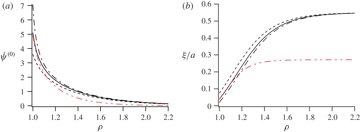
The normalized order-parameter (a) and correlation length (b) are plotted against the dimensionless radial distance  $\unicode[STIX]{x1D70C}\equiv r/a$. Dash, solid and dot-dash curves represent the results for
 $\unicode[STIX]{x1D709}_{\infty }/a=0.55$ and, respectively, for
 ${\hat{h}}=24$,
 $60$ and
 $150$. The two-dot chain (red) curve represents the result for
 $\unicode[STIX]{x1D709}_{\infty }/a=0.27$ and
 ${\hat{h}}=60$.

Figure 1 shows how the equilibrium order-parameter profile and the local correlation length depend on  $\unicode[STIX]{x1D70C}=r/a$. Far from the particle, the former approaches zero, which represents the critical composition, and the latter approaches the prescribed value of
 $\unicode[STIX]{x1D709}_{\infty }/a$. Near the particle surface, the preferred component is more concentrated and the correlation length becomes smaller as
 ${\hat{h}}$ increases. The stronger adsorption makes the mixture near the surface more off-critical. At a distance of
 $\unicode[STIX]{x1D709}_{\infty }$ from the particle surface,
 $\unicode[STIX]{x1D713}^{(0)}$ is approximately reduced to
 $\unicode[STIX]{x1D713}_{a}$. The local correlation length
 $\unicode[STIX]{x1D709}$ should be smaller than the local length scale that the flow changes, denoted here by
 $l$, for the validity of the hydrodynamics formulated from the coarse-grained free-energy density. In the flow at a distance
 $r$ from the centre of a particle moving translationally,
 $l$ would be equal or larger than
 $r$. In figure 1(b),
 $\unicode[STIX]{x1D709}$ is significantly small as compared with
 $r$. Thus, the hydrodynamics in the present formulation is valid in calculating the drag coefficient for the parameter values examined.
It is known that the Gaussian free-energy density can describe the static properties only when the mixture is not so close to the critical point. The proportionality of  $\unicode[STIX]{x1D709}\propto \unicode[STIX]{x1D70F}^{-\unicode[STIX]{x1D708}}$ with
 $\unicode[STIX]{x1D708}\approx 0.627$ is observed in the bulk of a binary fluid mixture with the critical composition when it is sufficiently close to the critical point. The Gaussian free-energy density, giving
 $\unicode[STIX]{x1D709}\propto \unicode[STIX]{x1D70F}^{-0.5}$ instead, appears to be valid when
 $\unicode[STIX]{x1D709}$ is smaller than approximately
 $15$ nm in the bulk of the mixture of 2,6-lutidine and water (Jungk, Belkoura & Woermann Reference Jungk, Belkoura and Woermann1987). When the particle motion is studied in the Gaussian model (Okamoto et al. Reference Okamoto, Fujitani and Komura2013; Fujitani Reference Fujitani2018), the correlation length is assumed to be homogeneous and much smaller than the minimum of
 $l$, i.e. approximately
 $a$, for the validity of the hydrodynamics based on the free-energy density. Thus, the Gaussian model is valid for small
 $\unicode[STIX]{x1D709}_{\infty }$ (
 ${<}15$ nm in the example above) and
 $\unicode[STIX]{x1D709}_{\infty }/a\ll 1$. The present formulation is not tied to these constraints.
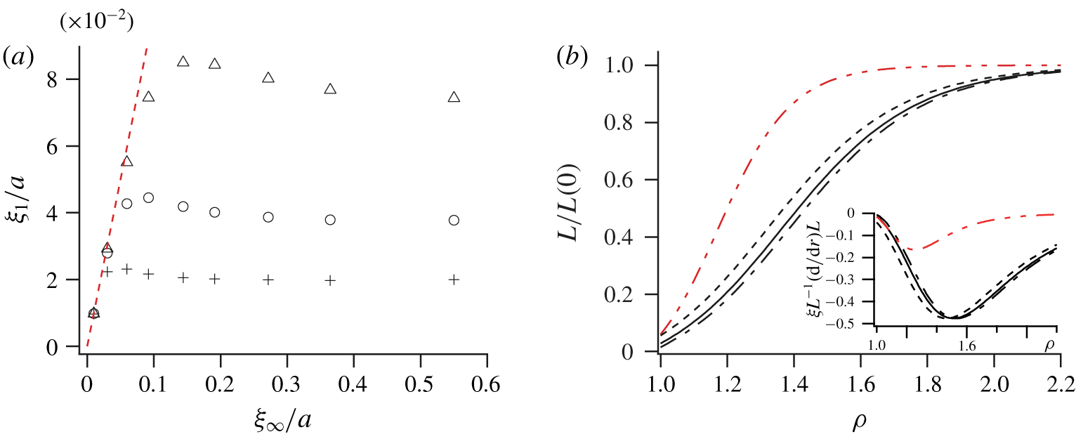
In figure 2(a),  $\unicode[STIX]{x1D709}$ at the surface (denoted by
 $\unicode[STIX]{x1D709}_{1}$) is approximately equal to
 $\unicode[STIX]{x1D709}_{\infty }$ for small
 $\unicode[STIX]{x1D709}_{\infty }/a$, and reaches a plateau after a slight peak as
 $\unicode[STIX]{x1D709}_{\infty }/a$ increases. The plateau of
 $\unicode[STIX]{x1D709}_{1}$ indicates that
 $\hat{\unicode[STIX]{x1D713}}^{(0)}$ at the surface becomes independent of
 $\unicode[STIX]{x1D709}_{\infty }/a$. The discrepancy between
 $\unicode[STIX]{x1D709}_{1}$ and
 $\unicode[STIX]{x1D709}_{\infty }$ implies the inhomogeneity in
 $\unicode[STIX]{x1D709}$, and cannot be described by the Gaussian model. As
 ${\hat{h}}$ increases in figure 2(a), the inhomogeneity appears at smaller
 $\unicode[STIX]{x1D709}_{\infty }/a$ and the plateau value is smaller, which is expected because the preferential adsorption causes the inhomogeneity. At the critical point (
 $\unicode[STIX]{x1D709}_{\infty }=\infty$), the equilibrium profile around a spherical particle is calculated in Yabunaka & Onuki (Reference Yabunaka and Onuki2017), where
 $\unicode[STIX]{x1D709}_{1}/a$ is found to be given by
 $6^{-1/3}{\hat{h}}^{-2/3}$ for
 ${\hat{h}}\gg 1$. This theoretical result, respectively, gives
 $\unicode[STIX]{x1D709}_{1}/a=6.6,3.6$ and
 $1.9\times 10^{-2}$ for
 ${\hat{h}}=24,60$ and
 $150$. The values of
 $\unicode[STIX]{x1D709}_{1}/a$ on the extreme right in figure 2(a) are
 $7.4,3.8$ and
 $2.0\times 10^{-2}$ for these values of
 ${\hat{h}}$, respectively. The latter two agree well with the corresponding theoretical results, showing the strong adsorption (
 $\unicode[STIX]{x1D70F}\ll \unicode[STIX]{x1D714}$ at the surface). Depending on the values of
 $a$ and
 ${\hat{h}}$, it is possible that the inhomogeneity occurs to invalidate the Gaussian model even when the Gaussian free-energy density gives good approximation to static properties in the bulk. Judging from figure 2(a), when
 $a$ equals 100 nm, the inhomogeneity begins to occur at the value of
 $\unicode[STIX]{x1D709}_{\infty }$ smaller than 10 nm for the strong adsorption. At this small value of
 $\unicode[STIX]{x1D709}_{\infty }$, the Gaussian free-energy density can describe the correlation length in the bulk of the mixture of 2,6-lutidine and water, which is mentioned in the preceding paragraph and is also discussed in § 6.
The Onsager coefficient  $L(\unicode[STIX]{x1D713}^{(0)})$ increases as
 $\unicode[STIX]{x1D713}^{(0)}$ approaches zero, which is shown in figure 2(b). At a distance of
 $\unicode[STIX]{x1D709}_{\infty }$ from the particle surface,
 $L(\unicode[STIX]{x1D713}^{(0)}(r))$ increases to become approximately
 $70\,\%$ of its value far from the particle,
 $L(0)$. Judging from figures 1(a) and 2(b), as is known,
 $\unicode[STIX]{x1D709}_{\infty }$ gives a typical thickness of the adsorption layer. The inset of figure 2(b) shows
 $\unicode[STIX]{x1D709}L^{-1}\,\text{d}L/(\text{d}r)$, whose absolute value represents how large the variation of
 $L(\unicode[STIX]{x1D713})$ over
 $\unicode[STIX]{x1D709}$, mentioned below (4.11), is as compared with the local value of
 $L(\unicode[STIX]{x1D713})$. The absolute value is sufficiently small for
 ${\hat{h}}=60$ over the region of
 $\unicode[STIX]{x1D70C}$ examined, while it is still smaller than unity but becomes rather large around
 $\unicode[STIX]{x1D70C}=1.5$ for
 ${\hat{h}}=150$.
(a) The normalized correlation length at the particle surface  $\unicode[STIX]{x1D709}_{1}/a$ is plotted against
 $\unicode[STIX]{x1D709}_{\infty }/a$ for
 ${\hat{h}}=24$ (▵), 60 (○) and
 $150$ (
 $+$). The dash line (red) represents
 $\unicode[STIX]{x1D709}_{1}=\unicode[STIX]{x1D709}_{\infty }$. (b) The ratio
 $L(\unicode[STIX]{x1D713}^{(0)}(\unicode[STIX]{x1D70C}a))/L(0)$ is plotted against
 $\unicode[STIX]{x1D70C}$. The normalized change of
 $L(\unicode[STIX]{x1D713}^{(0)}(r))$ over
 $\unicode[STIX]{x1D709}$, represented by
 $\unicode[STIX]{x1D709}L^{-1}\,\text{d}L/(\text{d}r)$, is plotted against
 $\unicode[STIX]{x1D70C}\equiv r/a$ in the inset. The parameter values for each curve are the same as used in figure 1.

5 Results
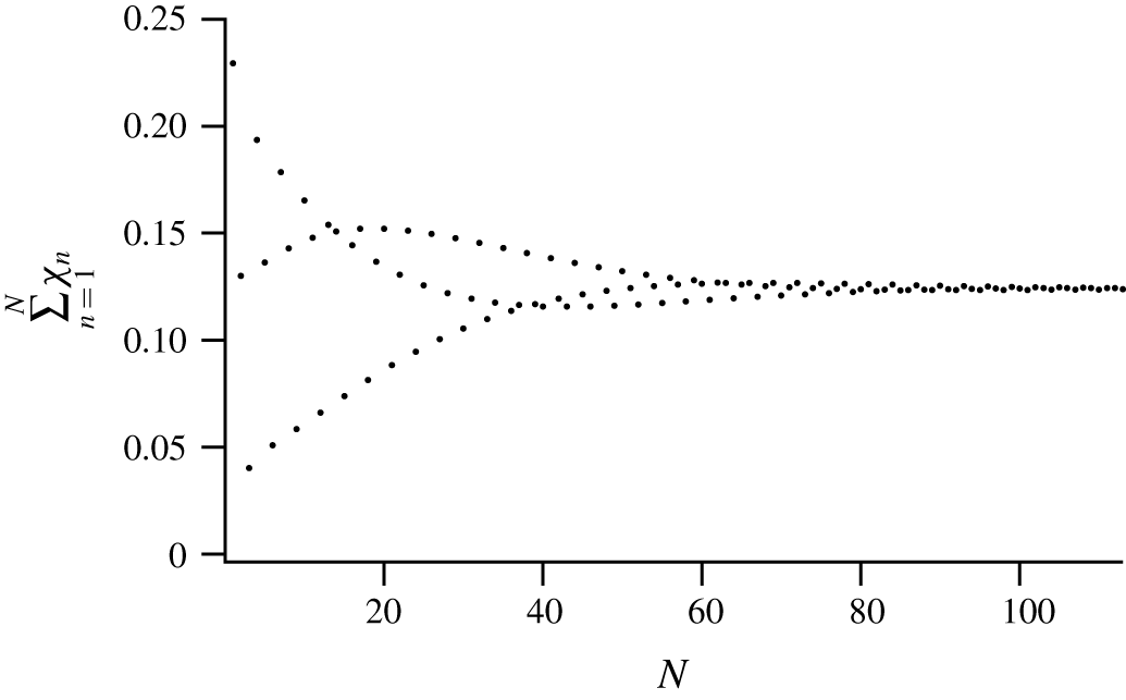
We truncate (4.8) appropriately to calculate  $\unicode[STIX]{x0394}\hat{\unicode[STIX]{x1D6FE}}_{d}$. The change of the partial sum occurring when the number of the terms
 $(N)$ increases by one becomes smaller than
 $1\,\%$ of the partial sum for
 $N\geqslant 109$ in figure 3. In this example, we can regard the partial sum of
 $N=109$ as the infinite sum. As
 ${\hat{h}}$ or
 $\unicode[STIX]{x1D709}_{\infty }/a$ increases, we need a larger
 $N$ to evaluate the infinite sum with the same accuracy, although the data are not shown. The numerical results shown later are obtained using
 $N$ smaller than approximately
 $100$. Some improvements to reduce the numerical cost are desirable when
 $N$ is required to be significantly larger than
 $100$.
Plot of  $\unicode[STIX]{x1D712}_{1}+\unicode[STIX]{x1D712}_{2}+\cdots +\unicode[STIX]{x1D712}_{N}$ against
 $N$ for
 ${\hat{h}}=150$ and
 $\unicode[STIX]{x1D709}_{\infty }/a=0.36$.

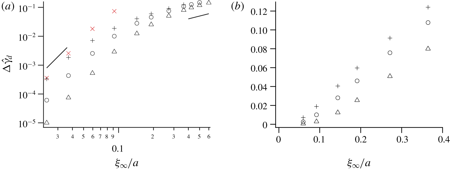
It is shown in figure 4 how  $\unicode[STIX]{x0394}\hat{\unicode[STIX]{x1D6FE}}_{d}$ changes as the critical temperature is approached. The deviation increases with
 ${\hat{h}}$ and
 $\unicode[STIX]{x1D709}_{\infty }/a$, as is expected because it is caused by the adsorption. In this figure, for small
 $\unicode[STIX]{x1D709}_{\infty }/a$,
 $\unicode[STIX]{x0394}\hat{\unicode[STIX]{x1D6FE}}_{d}$ appears to be approximately proportional to the fourth power of
 $\unicode[STIX]{x1D709}_{\infty }/a$. As
 $\unicode[STIX]{x1D709}_{\infty }/a$ increases in figure 4(a), the slope shown by each of the symbols,
 $+$,
 $\circ$ and
 $\triangle$, becomes more gradual and the dependence appears to shift to the linear dependence; the shift occurs at larger
 $\unicode[STIX]{x1D709}_{\infty }/a$ as
 ${\hat{h}}$ decreases. For large
 $\unicode[STIX]{x1D709}_{\infty }/a$ in figure 4(b),
 $\unicode[STIX]{x0394}\hat{\unicode[STIX]{x1D6FE}}_{d}$ appears to be a linear function of
 $\unicode[STIX]{x1D709}_{\infty }/a$, whose slope is calculated from the two data points on the right-hand end to give
 $0.31$,
 $0.34$ and
 $0.35$ for
 ${\hat{h}}=24,~60$ and
 $150$, respectively. This suggests that the slope should become insensitive to
 ${\hat{h}}$ as
 $\unicode[STIX]{x1D709}_{\infty }/a$ increases. The approximate fourth-power dependence for smaller
 $\unicode[STIX]{x1D709}_{\infty }/a$, shown in figure 4(a), is mentioned at the end of the penultimate paragraph of § 4 of Fujitani (Reference Fujitani2018), where the Gaussian model is studied and the parameter
 $\unicode[STIX]{x1D6EC}({\approx}{\hat{h}}/\sqrt{5\unicode[STIX]{x03C0}})$ is used. For reference in figure 4(a), using the calculation procedure in Fujitani (Reference Fujitani2018), we plot the normalized deviation in the Gaussian model, corresponding with
 $\unicode[STIX]{x0394}\hat{\unicode[STIX]{x1D6FE}}_{d}$, for
 ${\hat{h}}=150$; the results (
 $\times$) deviate upward from the results of the present study (
 $+$) as
 $\unicode[STIX]{x1D709}_{\infty }/a$ increases.
(a) Logarithmic and (b) linear plots of the normalized deviation of the drag coefficient  $\unicode[STIX]{x0394}\hat{\unicode[STIX]{x1D6FE}}_{d}$ against
 $\unicode[STIX]{x1D709}_{\infty }/a$ for
 ${\hat{h}}=24$ (▵), 60 (○) and 150 (
 $+$). Each of the results is obtained using a partial sum of (4.8). Lines in (a) represent the slopes of one and four. The symbol
 $\times$ (red) in (a) represents the results in the Gaussian model for
 ${\hat{h}}=150$.

By assuming  $L$ to be homogeneous, instead of using (4.11), we calculate
 $\unicode[STIX]{x0394}\hat{\unicode[STIX]{x1D6FE}}_{d}$ to obtain the results shown by
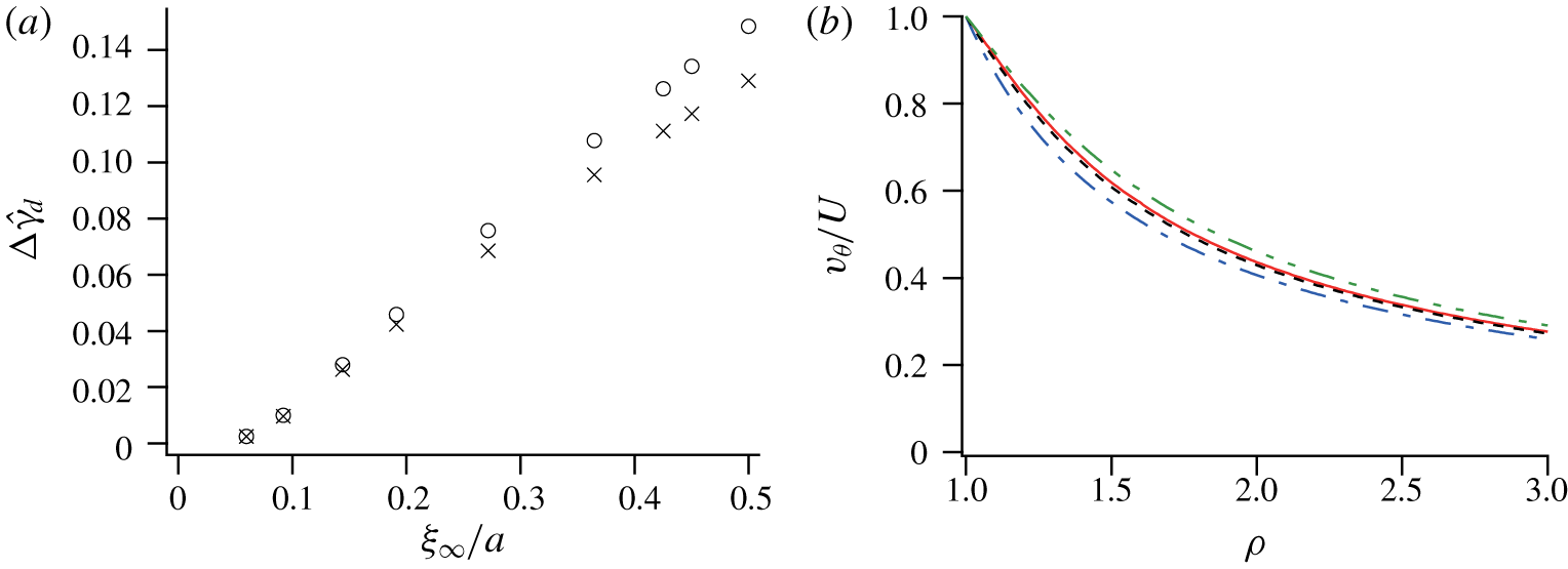
 $\times$ in figure 5(a). This drastic change in modelling
 $L$ does not influence
 $\unicode[STIX]{x0394}\hat{\unicode[STIX]{x1D6FE}}_{d}$ for smaller values of
 $\unicode[STIX]{x1D709}_{\infty }/a$, and reduces
 $\unicode[STIX]{x0394}\hat{\unicode[STIX]{x1D6FE}}_{d}$ slightly as
 $\unicode[STIX]{x1D709}_{\infty }/a$ increases. It is still that the dependence of
 $\unicode[STIX]{x0394}\hat{\unicode[STIX]{x1D6FE}}_{d}$ on
 $\unicode[STIX]{x1D709}_{\infty }/a$ becomes more gradual than in the Gaussian model. We thus expect that the appearance of the gradual dependence should be robust against the details of the dependence of
 $L$ on
 $\unicode[STIX]{x1D713}$, although the results in the inset of figure 2(b) suggest that (4.11) is not completely reliable especially for
 ${\hat{h}}=150$.
As mentioned in § 1, some researchers regard the deviation of  $\unicode[STIX]{x1D6FE}_{d}$ to be caused by the effective enlargement of the particle radius due to the adsorption layer. However, for the parameter values examined in figure 5(b), the change of
 $v_{\unicode[STIX]{x1D703}}/U$ at
 $\unicode[STIX]{x1D703}=\unicode[STIX]{x03C0}/2$ due to the preferential adsorption is smaller than approximately
 $20\,\%$ of
 $v_{\unicode[STIX]{x1D703}}/U$ in its absence; the velocity field is not much changed by the preferential adsorption and the mixture fluid in the adsorption layer cannot be regarded as a part of the rigid particle. The velocity gradient at the surface becomes more gradual as
 $\unicode[STIX]{x1D709}_{\infty }/a$ increases, which suggests reduction in the viscous stress exerted on the particle. The velocity field is influenced by
 $\unicode[STIX]{x1D72B}$ because of (3.11) and (3.12). How
 $\unicode[STIX]{x1D72B}$ changes with
 $\unicode[STIX]{x1D709}_{\infty }/a$ influences on how
 $\unicode[STIX]{x0394}\hat{\unicode[STIX]{x1D6FE}}_{d}$ changes with
 $\unicode[STIX]{x1D709}_{\infty }/a$ not only directly through the first term in parentheses of (3.26) but also through the last two terms by changing the flow field.
The dependence of  $\unicode[STIX]{x0394}\hat{\unicode[STIX]{x1D6FE}}_{d}$ on
 $\unicode[STIX]{x1D709}_{\infty }/a$ becomes close to the linear one in figure 4(a) in the range of
 $({\hat{h}},\unicode[STIX]{x1D709}_{\infty }/a)$ showing the inhomogeneity of
 $\unicode[STIX]{x1D709}$ in figure 2(a). This is reasonable because of the close relationship between
 $\unicode[STIX]{x1D713}^{(0)}$ and
 $\unicode[STIX]{x0394}\unicode[STIX]{x1D6FE}_{d}$ shown by (3.28). In figure 2(a), the inhomogeneity occurs approximately when
 $\unicode[STIX]{x1D709}_{1}/a$ exceeds
 $\unicode[STIX]{x1D709}_{\infty }/a$. Thus, when large
 ${\hat{h}}$ causes the strong adsorption, the dependence in figure 4(a) becomes close to the linear one if we have
 $$\begin{eqnarray}\frac{\unicode[STIX]{x1D709}_{\infty }}{a}>6^{-1/3}{\hat{h}}^{-2/3}.\end{eqnarray}$$
(a) The normalized deviation  $\unicode[STIX]{x0394}\hat{\unicode[STIX]{x1D6FE}}_{d}$ is obtained for
 ${\hat{h}}=60$ by assuming (4.11) (○) and by assuming
 $L$ to be homogeneous (
 $\times$). Some of the results shown by ○ are shared with figure 4. (b) The tangential component of the velocity field
 $v_{\unicode[STIX]{x1D703}}$ divided by
 $U$ is plotted against
 $\unicode[STIX]{x1D70C}$ on the equatorial plane
 $\unicode[STIX]{x1D703}=\unicode[STIX]{x03C0}/2$. The dot-dash curve (blue) represents the results in the absence of the preferential adsorption (
 $h=0$). Dash, solid and two-dot chain curves (black, red, and green, respectively) represent the results for
 $({\hat{h}},\unicode[STIX]{x1D709}_{\infty }/a)=(60,0.19)$,
 $(150,0.19)$ and
 $(60,0.36)$, respectively.

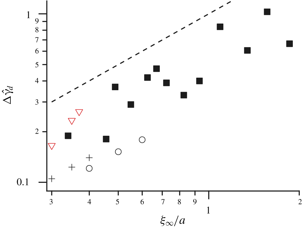
Solid squares represent part of the data in the top of figure 2 of Omari et al. (Reference Omari, Grabowski and Mukhopadhyay2009). Circles and crosses represent our results calculated with  $\unicode[STIX]{x1D702}=0.036$ for
 ${\hat{h}}=60$ and
 $150$, respectively. The calculated values are slightly larger for large
 $\unicode[STIX]{x1D709}_{\infty }/a$ than the ones obtained with
 $\unicode[STIX]{x1D702}=0$. For
 $({\hat{h}},\unicode[STIX]{x1D709}_{\infty }/a)=(60,0.4)$ and
 $(60,0.5)$, we have
 $\unicode[STIX]{x0394}\hat{\unicode[STIX]{x1D6FE}}_{d}=0.119\,(0.121)$ and
 $0.148\,(0.152)$ by using
 $\unicode[STIX]{x1D702}=0\,(0.036)$, respectively. The triangles (red) represent the results for
 ${\hat{h}}=24$ in the Gaussian model. The dash line represents
 $\unicode[STIX]{x0394}\hat{\unicode[STIX]{x1D6FE}}_{d}=\unicode[STIX]{x1D709}_{\infty }/a$.

6 Discussion
The Gaussian free-energy density was used in the previous studies on the drag coefficient (Okamoto et al. Reference Okamoto, Fujitani and Komura2013; Fujitani Reference Fujitani2018). There,  $\unicode[STIX]{x1D709}_{\infty }$ should be sufficiently small so that the free-energy density can describe the static properties in the bulk and so that the correlation length can be regarded as homogeneous. The latter condition can require smaller
 $\unicode[STIX]{x1D709}_{\infty }$ than the former unless the adsorption is weak. Thus, the Gaussian model is not always valid in calculating
 $\unicode[STIX]{x1D6FE}_{d}$ even if the static properties in the mixture bulk can be described by the Gaussian free-energy density, as mentioned in § 4.3. The free-energy density in (3.1) is completely free from these conditions because it can describe the static properties in the bulk even at the critical point and the inhomogeneity of
 $\unicode[STIX]{x1D709}$. This inhomogeneity is correlated with the appearance of the approximate linearity between
 $\unicode[STIX]{x0394}\hat{\unicode[STIX]{x1D6FE}}_{d}$ and
 $\unicode[STIX]{x1D709}_{\infty }/a$, which should occur for large
 $\unicode[STIX]{x1D709}_{\infty }/a$ satisfying (5.1).
Omari et al. (Omari et al. Reference Omari, Grabowski and Mukhopadhyay2009) measured the self-diffusion of silica particles in a near-critical mixture of 2,6-lutidine and water, for which  $T_{c}$ is approximately 307 K (Gülari et al. Reference Gülari, Collings, Schmidt and Pings1972; Jungk et al. Reference Jungk, Belkoura and Woermann1987). The former is preferentially adsorbed by the particle, and the self-diffusion coefficient is suppressed as
 $T_{c}$ is approached. The data on the top of figure 2 of Omari et al. (Reference Omari, Grabowski and Mukhopadhyay2009), except the data point on the extreme left, are replotted in figure 6;
 $a=25~\text{nm}$ and
 $\unicode[STIX]{x1D709}_{0}=0.25~\text{nm}$ used in this reference lead to
 $\unicode[STIX]{x1D70F}_{a}=6.5\times 10^{-4}$. We thus have
 $\unicode[STIX]{x1D709}_{\infty }/a=0.76$ for
 $\unicode[STIX]{x1D70F}=10^{-3}$; the replotted data range from
 $\unicode[STIX]{x1D70F}=3.6\times 10^{-3}$ to
 $2.3\times 10^{-4}$. Equations (4.15) and (4.16) give
 ${\hat{h}}=h\sqrt{3u^{\ast }a^{3}}/(k_{B}T_{c}\sqrt{C_{1}})$ for
 $\unicode[STIX]{x1D702}=0$. The value of
 $h$ may be usually smaller than
 $10^{-5}~\text{m}^{3}~\text{s}^{-2}$, considering the following three points: (i) a typical energy of the hydrogen bond is
 $10^{-20}~\text{J}$ per a molecule, (ii) the area of the particle surface interacting with one molecule of the mixture would be larger than approximately
 $1~\text{nm}^{2}$, and (iii)
 $|\unicode[STIX]{x1D713}|$ is at most
 $10^{3}~\text{kg}~\text{m}^{-3}$. Using a typical value of
 $M$ for alkanes,
 $10^{-16}~\text{m}^{7}~\text{kg}^{-1}~\text{s}^{-2}$ (Carey, Scriven & Davis Reference Carey, Scriven and Davis1980; Cornelisse, Peters & de Swaan Arons Reference Cornelisse, Peters and de Swaan Arons1996), we find that
 ${\hat{h}}$ is smaller than approximately
 $160$. We use a partial sum of (4.8) with
 $\unicode[STIX]{x1D702}=0.036$ to calculate
 $\unicode[STIX]{x0394}\hat{\unicode[STIX]{x1D6FE}}_{d}$, and plot the results for small values of
 $\unicode[STIX]{x1D709}_{\infty }/a$ in figure 6. We did not calculate
 $\unicode[STIX]{x0394}\hat{\unicode[STIX]{x1D6FE}}_{d}$ at values of
 $\unicode[STIX]{x1D709}_{\infty }/a$ larger than shown in the figure for each of
 ${\hat{h}}=60$ and
 $150$ because of the heavy numerical costs. The calculation results for
 $h=60$ and
 $150$ appear to have almost the same slopes with the slope suggested by the experimental data. However, judging from figure 6, the calculation would yield smaller
 $\unicode[STIX]{x0394}\hat{\unicode[STIX]{x1D6FE}}_{d}$ than the experimental data, even if performed for the same values of
 $\unicode[STIX]{x1D709}_{\infty }/a$ that give the experimental data. The underestimation may be attributed to our assumption of homogeneous viscosity.
The singular part of the viscosity is proportional to  $\unicode[STIX]{x1D709}^{1/19}$ up to the 1-loop order (Ohta Reference Ohta1975; Ohta & Kawasaki Reference Ohta and Kawasaki1976; Siggia et al. Reference Siggia, Hohenberg and Halperin1976). Thus, its non-universal regular part, which can depend on the local composition, is not negligible unless the mixture is very close to the critical point. We can estimate
 $\unicode[STIX]{x1D713}_{a}\approx 15~\text{kg}~\text{m}^{-3}$ for the parameter values mentioned above, using (3.3), (3.6) and (4.15). Considering that the mass density of 2,6-lutidine (
 $0.93~\text{g}~\text{cm}^{-3}$) is almost the same as that of water, the change of
 $5\,\%$ in the weight per cent of 2,6-lutidine in the mixture approximately amounts to that of
 $7$ in
 $\hat{\unicode[STIX]{x1D713}}^{(0)}$. In figure 1(a), the values of
 $\hat{\unicode[STIX]{x1D713}}^{(0)}$ at the surface are approximately
 $5$ and
 $7$ for
 ${\hat{h}}=60$ and
 $150$ for
 $\unicode[STIX]{x1D709}_{\infty }/a=0.55$, respectively. The data of the viscosity for various values of the weight per cent are shown at
 $\unicode[STIX]{x1D70F}\approx 10^{-2}$ and
 $10^{-4}$ in (Stein et al. Reference Stein, Davidson, Allegra and Allen1972). From them, in the experimental system yielding the data replotted in figure 6, the viscosity near the surface is guessed to be raised by approximately
 $30\,\%$ around
 $\unicode[STIX]{x1D70F}=10^{-3}$. It is thus possible that the underestimation suggested in figure 6 can be explained by this slight increase of the viscosity in the adsorption layer. The viscosity may be regarded as homogeneous over the mixture around
 $\unicode[STIX]{x1D70F}=10^{-4}$ due to the overlap of the regular and singular parts, according to the data in Stein et al. (Reference Stein, Davidson, Allegra and Allen1972). These data also suggest that, when
 $\unicode[STIX]{x1D70F}$ is smaller than
 $10^{-4}$, or
 $\unicode[STIX]{x1D709}_{\infty }$ is larger than approximately 80 nm, the singular part should become more explicit to cause inhomogeneous viscosity.
The results in the Gaussian model for  ${\hat{h}}=150$ in figure 4(a) are obtained using a series expansion with respect to the dimensionless parameter proportional to
 $h$, which is mentioned in the preface of § 4; the series is given by the first entry of (47) in Fujitani (Reference Fujitani2018). For
 ${\hat{h}}=24,60$ and
 $150$, respectively, when
 $\unicode[STIX]{x1D709}_{\infty }/a$ is larger than approximately
 $0.4$,
 $0.18$ and
 $0.1$, the drag coefficient cannot be calculated in the Gaussian model because the expansion series is numerically divergent. Results in the Gaussian model for
 ${\hat{h}}=24$ are plotted with triangles in figure 6. For
 ${\hat{h}}=60$ and
 $\unicode[STIX]{x1D709}_{\infty }/a=0.14$, the normalized deviation in the Gaussian model is
 $8.3\times 10^{-2}$, and is larger than the corresponding result shown by a circle in figure 4(a). Thus, as far as examined, the dependence of the normalized deviation of the drag coefficient on
 $\unicode[STIX]{x1D709}_{\infty }/a$ in the Gaussian model does not become close to the linear one, in contrast to our results calculated with the renormalized local functional theory. It is to be noted that, judging from figure 2(a), the Gaussian model loses validity for
 ${\hat{h}}=24,60$ and
 $150$ in the range of
 $\unicode[STIX]{x1D709}_{\infty }/a$ of figure 6. It is thus only for reference that the results in the Gaussian model are plotted in this figure. If the particle were enlarged by the thickness of the adsorption layer, we would have
 $\unicode[STIX]{x0394}\hat{\unicode[STIX]{x1D6FE}}_{d}=\unicode[STIX]{x1D709}_{\infty }/a$, which is also plotted for reference in figure 6. This naive idea clearly oversimplifies the dynamics of the mixture; it is suggested by figure 5(b) that the mixture generally flows in the adsorption layer. That the dash line lies above the experimental data in figure 6 may imply that the naive idea could be justified approximately if the preferred component were extremely viscous.
The particle radius in the experiment is rather small. For  $a=25~\text{nm}$, our coarse-grained picture should become less reliable very near the surface because
 $\unicode[STIX]{x1D709}_{1}$ reaches a microscopic length scale in figure 1(b). Our theory can be safely applied to a particle radius larger than approximately 100 nm. Lee (Lee Reference Lee1976) measured the self-diffusion coefficient of such large particles in a ternary mixture near the plait point, and found out the linear dependence of
 $\unicode[STIX]{x0394}\hat{\unicode[STIX]{x1D6FE}}_{d}$ on
 $\unicode[STIX]{x1D709}_{\infty }/a$ when
 $\unicode[STIX]{x1D70F}$ is approximately smaller than
 $3\times 10^{-2}$ (i.e.
 $\unicode[STIX]{x1D709}_{\infty }\gtrsim 5~\text{nm}$). For this mixture, the renormalized local functional theory is valid if
 $\unicode[STIX]{x1D70F}$ is replaced by a variable proportional to
 $\unicode[STIX]{x1D70F}^{1/(1-\unicode[STIX]{x1D6FC})}$ (Fisher Reference Fisher1968; Folk & Moser Reference Folk and Moser1995), although the definition of the surface field and (3.13) should be modified for ternary mixtures.
In figure 1(b),  $\unicode[STIX]{x1D709}$ is much smaller than
 $a$ near the particle, and increases to approach
 $\unicode[STIX]{x1D709}_{\infty }$ mainly in the region of
 $r-a<\unicode[STIX]{x1D709}_{\infty }$. Thus, for the parameter values examined,
 $\unicode[STIX]{x1D709}$ nowhere exceeds the length scale that the flow changes (
 $l$), which would be equal or larger than
 $r$. In particular when the adsorption is strong, the local correlation length near the particle is much smaller than the particle radius. Thus, when we consider a large particle (
 $a\gtrsim 100~\text{nm}$) with strong adsorption in a near-critical mixture whose
 $\unicode[STIX]{x1D709}_{\infty }$ is not so large as to cause the explicit singular part of the viscosity (
 $\unicode[STIX]{x1D709}_{\infty }<80~\text{nm}$ in the mixture mentioned above),
 $l$ is sufficiently large as compared with
 $\unicode[STIX]{x1D709}$ everywhere. Then, we can use the present hydrodynamic formulation based on the coarse-grained free-energy density in calculating the drag coefficient, without considering the critical fluctuations significant on length scales smaller than
 $\unicode[STIX]{x1D709}$.
We use  $\unicode[STIX]{x1D700}$ as a convenient parameter to calculate the drag coefficient up to linear order with respect to the particle speed. The parameter is taken as representing the Reynolds number in deriving the conventional Stokes law, which holds for low Reynolds number, as mentioned in § 2. Thus, we can discuss the validity range of the linear regime by making the physical meaning of
 $\unicode[STIX]{x1D700}$ explicit. In the presence of the preferential adsorption in the near criticality, the low Reynolds number should remain required for the linearity, but it would not be sufficient because nonlinearity is suggested to be made relevant by significant distortion of the adsorption layer due to the particle motion (Furukawa et al. Reference Furukawa, Gambassi, Dietrich and Tanaka2013). The distortion would be reduced by the mutual diffusion of the two fluid components, while augmented by the convection. The time scale that the former occurs over the adsorption layer can be estimated to be
 $(a+\unicode[STIX]{x1D709}_{\infty })^{2}/D$, where
 $D$ is the diffusion coefficient given by the fraction in (4.10), while the one for the latter can be estimated to be
 $a+\unicode[STIX]{x1D709}_{\infty }$ divided by the particle speed
 $U_{o}$. Thus,
 $\unicode[STIX]{x1D700}$ in our problem would be taken as representing not only the Reynolds number but also the Péclet number,
 $(a+\unicode[STIX]{x1D709}_{\infty })U_{o}/D$, which increases with
 $\unicode[STIX]{x1D709}_{\infty }$. It is to be noted that we calculate the drag force by taking into account the distortion of the adsorption layer, as mentioned above (3.27). However, elucidating the validity range should require calculating beyond the linear regime and checking the linearity for various values of the parameters including
 $\unicode[STIX]{x1D709}_{\infty }$. To examine whether the Brownian motion can be described by a linear Langevin equation, we may need to study the drag force beyond the linear regime in the framework of the fluctuating hydrodynamics, considering that a Brownian particle does not always move translationally in a quiescent fluid. It is thus well expected that the self-diffusion coefficient of a Brownian particle should not always follow Einstein’s relation, i.e. should not be always given by
 $k_{B}T/\unicode[STIX]{x1D6FE}_{d}$, even when the Reynolds number is sufficiently small. The relation can break down when
 $\unicode[STIX]{x1D709}_{\infty }/a$ is sufficiently large. We believe that our results of the drag coefficient should also give a firm basis to some future work, experimental or theoretical, on the validity range of
 $\unicode[STIX]{x1D709}_{\infty }/a$ for Einstein’s relation in the presence of preferential adsorption in the near-criticality.
Acknowledgements
S.Y. was supported by Grant-in-Aid for Young Scientists (B) (15K17737 and 18K13516).
Appendix A. Some details
The kernel appearing in (3.24) is given by
 $$\begin{eqnarray}\unicode[STIX]{x1D6E4}_{R}(\unicode[STIX]{x1D70C},\unicode[STIX]{x1D70E})=\left\{\begin{array}{@{}ll@{}}\displaystyle \frac{(3-5\unicode[STIX]{x1D70E}^{2})}{2\unicode[STIX]{x1D70E}^{3}\unicode[STIX]{x1D70C}^{3}}+5\frac{(3\unicode[STIX]{x1D70E}^{2}-1)}{2\unicode[STIX]{x1D70E}^{3}\unicode[STIX]{x1D70C}}+\unicode[STIX]{x1D70E}^{2}\unicode[STIX]{x1D70C}^{-3}-5\unicode[STIX]{x1D70C}^{-1},\quad & \unicode[STIX]{x1D70C}\geqslant \unicode[STIX]{x1D70E}\\ \displaystyle \frac{(3-5\unicode[STIX]{x1D70E}^{2})}{2\unicode[STIX]{x1D70E}^{3}\unicode[STIX]{x1D70C}^{3}}+5\frac{(3\unicode[STIX]{x1D70E}^{2}-1)}{2\unicode[STIX]{x1D70E}^{3}\unicode[STIX]{x1D70C}}+\unicode[STIX]{x1D70C}^{2}\unicode[STIX]{x1D70E}^{-3}-5\unicode[STIX]{x1D70E}^{-1},\quad & \unicode[STIX]{x1D70E}\geqslant \unicode[STIX]{x1D70C}.\end{array}\right.\end{eqnarray}$$
We find
 $$\begin{eqnarray}\left({\textstyle \frac{1}{2}}\unicode[STIX]{x2202}_{\unicode[STIX]{x1D70C}}^{3}+2\unicode[STIX]{x2202}_{\unicode[STIX]{x1D70C}}^{2}\right)\unicode[STIX]{x1D6E4}_{R}(\unicode[STIX]{x1D70C},\unicode[STIX]{x1D70E})=15[\unicode[STIX]{x1D6FC}_{0}(\unicode[STIX]{x1D70E})+1],\end{eqnarray}$$
at  $\unicode[STIX]{x1D70C}=1$. The operator in the parentheses above appears in (2.13). The kernel appearing in (3.25) is given by
 $$\begin{eqnarray}\displaystyle \unicode[STIX]{x1D6E4}_{Q}(\unicode[STIX]{x1D70C},\unicode[STIX]{x1D70E})=\left\{\begin{array}{@{}ll@{}}(\unicode[STIX]{x1D70C}\unicode[STIX]{x1D70E})^{-2}/2+\unicode[STIX]{x1D70C}\unicode[STIX]{x1D70E}^{-2},\quad & \unicode[STIX]{x1D70C}\leqslant \unicode[STIX]{x1D70E}\\ (\unicode[STIX]{x1D70C}\unicode[STIX]{x1D70E})^{-2}/2+\unicode[STIX]{x1D70E}\unicode[STIX]{x1D70C}^{-2},\quad & \unicode[STIX]{x1D70E}\leqslant \unicode[STIX]{x1D70C}.\end{array}\right. & & \displaystyle\end{eqnarray}$$
These kernels are originally obtained in Okamoto et al. (Reference Okamoto, Fujitani and Komura2013).
We can calculate the equilibrium profile numerically by using (3.7) and (3.8), as they are, after the non-dimensionalization mentioned in § 4.3. Alternatively, we can utilize (A5) of Fujitani (Reference Fujitani2016), whose  $s(\unicode[STIX]{x1D713}(\unicode[STIX]{x1D70C}))$ is defined as
 $\unicode[STIX]{x1D714}(\unicode[STIX]{x1D713}(\unicode[STIX]{x1D70C}))/\unicode[STIX]{x1D70F}-1$ and becomes proportional to
 $e^{-2\unicode[STIX]{x1D70C}a/\unicode[STIX]{x1D709}_{\infty }}/\unicode[STIX]{x1D70C}^{2}$ far from the particle. The differential equation with respect to the ratio of the former to the latter, that is
 $s(\unicode[STIX]{x1D713}(\unicode[STIX]{x1D70C}))e^{2\unicode[STIX]{x1D70C}a/\unicode[STIX]{x1D709}_{\infty }}\unicode[STIX]{x1D70C}^{2}$, can be derived from (3.7), and is solved numerically under the boundary conditions imposed sufficiently far from the particle. At
 $\unicode[STIX]{x1D70C}=10$, we required the derivative of
 $s$ with respect to
 $\unicode[STIX]{x1D70C}$ to vanish, and fixed the value of
 $s$ so that
 ${\hat{h}}$ becomes a prescribed value with the aid of (3.8).