


1 INTRODUCTION
Tests and confidence intervals based on so-called heteroskedasticity robust standard errors date back to Eicker (Reference Eicker1963, Reference Eicker1967) and constitute, at least since White (Reference White1980), a major component of the applied econometrician’s toolbox. Although these early methods come with well-understood large sample properties, when based on critical values derived from asymptotic theory, their finite sample properties often deviate substantially from what asymptotic theory suggests: tests may substantially overreject under the null and corresponding confidence intervals may undercover. Strong leverage points have been identified early on as one major reason for these deviations (see, e.g., Davidson and MacKinnon, Reference Davidson and MacKinnon1985; MacKinnon and White, Reference MacKinnon and White1985; Chesher and Jewitt, Reference Chesher and Jewitt1987). This has led to various developments trying to attenuate such drawbacks:
-
1. modifications of the covariance matrix estimators in Eicker (Reference Eicker1963, Reference Eicker1967) and White (Reference White1980) led to tests based on what are now frequently called HC1–HC4 covariance matrix estimators (see, e.g., Long and Ervin, Reference Long and Ervin2000 and Cribari-Neto, Reference Cribari-Neto2004, for an overview of the relevant literature), with HC0 denoting the original proposal;
-
2. some authors investigated degree-of-freedom corrections to obtain modified critical values (e.g., Satterthwaite, Reference Satterthwaite1946 or Bell and McCaffrey, Reference Bell and McCaffrey2002, see also Imbens and Kolesár, Reference Imbens and Kolesár2016);
-
3. wild bootstrap methods were investigated (for an overview of the relevant literature, see Pötscher and Preinerstorfer, Reference Pötscher and Preinerstorfer2023) and, more recently, parametric bootstrap methods were studied in Chu et al. (Reference Chu, Lee, Ullah and Xu2021) and Hansen (Reference Hansen2021).
Although these developments sometimes lead to improvements, they come with no general finite sample guarantees concerning the size of the tests or the coverage of related confidence intervals (cf. the discussion in Pötscher and Preinerstorfer (Reference Pötscher and Preinerstorfer2023, Reference Pötscher and Preinerstorfer2025), for detailed accounts).
Motivated by this lack of finite sample guarantees, Pötscher and Preinerstorfer (Reference Pötscher and Preinerstorfer2025) studied the question under which conditions heteroskedasticity robust test statistics as well as the standard (uncorrected) F-test statistic can actually be paired with appropriate (finite) critical values, so that one obtains tests that have their (finite sample) size controlled by the prescribed significance value
$\alpha $
 (i.e., have size
$\leq \alpha $
 ) even though one is completely agnostic about the form of heteroskedasticity.Footnote
1
Under appropriate assumptions on the errors, allowing for Gaussian as well as substantial non-Gaussian behavior, they have shown that the standard (uncorrected) F-test statistic can be size-controlled (in finite samples) by using an appropriately chosen (finite) critical value if and only if the following simple condition holds:

see (8) in Pötscher and Preinerstorfer (Reference Pötscher and Preinerstorfer2025) for a formal statement of this condition.
Under a generally stronger condition than (1) (see (10) in Pötscher and Preinerstorfer, Reference Pötscher and Preinerstorfer2025), it was furthermore shown that large classes of heteroskedasticity robust test statistics (e.g., HC0–HC4) can be size-controlled by appropriate (finite) critical values. That condition, however, although satisfied for many testing problems (and even often identical to (1), cf. Theorem 3.9 and Lemma A.3 in Pötscher and Preinerstorfer, Reference Pötscher and Preinerstorfer2018), is not necessary in general, as shown in examples given in Pötscher and Preinerstorfer (Reference Pötscher and Preinerstorfer2025); for example, their Example 5.5 or Example C.1 in their Appendix C.Footnote 2 These examples consider the case of testing linear contrasts in the expected outcomes of subjects belonging to two or more groups, scenarios that are practically relevant. Further examples are provided in Examples A.1–A.4 in Appendix A further below.Footnote 3
For the important case of testing problems involving only a single restriction (i.e., the case
$q=1$
 in the notation of Pötscher and Preinerstorfer, Reference Pötscher and Preinerstorfer2025), we show in the present article that the condition in (1) is then in fact necessary and sufficient also for size controllability of the above-mentioned classes of heteroskedasticity robust test statistics, including HC0–HC4.
2 RESULTS ON SIZE CONTROLLABILITY
2.1 Framework
Here, we recall the most relevant notions from Sections 2 and 3 of Pötscher and Preinerstorfer (Reference Pötscher and Preinerstorfer2025), to which we refer the reader for further information and discussion. We consider the linear regression model

where X is a (real) nonstochastic regressor (design) matrix of dimension
$ n\times k$
 and
$\beta \in \mathbb {R}^{k}$
 denotes the unknown regression parameter vector. Throughout, we assume
$\mathrm {rank}(X)=k$
 and
$1\leq k<n$
 . We furthermore assume that the
$n\times 1$
 disturbance vector
$ \mathbf {U}=(\mathbf {u}_{1},\ldots ,\mathbf {u}_{n})^{\prime }$
 (
$\!\!\!^{\prime }$
 denoting transposition) has mean zero and unknown covariance matrix
$\sigma ^{2}\Sigma $
 (
$0<\sigma <\infty $
 ), where
$\Sigma $
 varies in the “heteroskedasticity model” given by

and
$\mathrm {diag}(\tau _{1}^{2},\ldots ,\tau _{n}^{2})$
 denotes the diagonal
$n\times n$
 matrix with diagonal elements given by
$\tau _{i}^{2}$
 . That is, the disturbances are uncorrelated but can be heteroskedastic of arbitrary form. (In Appendix B, we shall also consider another heteroskedasticity model.)Footnote
4
For ease of exposition, we shall maintain in the sequel that the disturbance vector
$\mathbf {U}$
 is normally distributed. Generalizations to classes of non-normal disturbances can be obtained following the arguments in Section 7.1 of Pötscher and Preinerstorfer (Reference Pötscher and Preinerstorfer2025), see Remark 2.2 further below. Denoting a Gaussian probability measure with mean
$\mu \in \mathbb {R}^{n}$
 and (possibly singular) covariance matrix A by
$P_{\mu ,A}$
 , the collection of distributions on
$\mathbb {R}^{n}$
 (the sample space of
$ \mathbf {Y}$
 ) induced by the linear model just described together with the Gaussianity assumption is then given by

where
${\mathrm {span}}(X)$
 denotes the column space of X.Footnote
5
We focus on testing the null
$R\beta =r$
 against the alternative
$R\beta \neq r$
 , where
$R\neq 0$
 is a
$1\times k$
 vector and
$r\in \mathbb {R}$
 . That is, throughout this article, we focus on testing a single restriction, whereas the theory developed in Pötscher and Preinerstorfer (Reference Pötscher and Preinerstorfer2025) allows for simultaneously testing multiple restrictions (i.e., we here consider only the special case corresponding to
$q=1$
 in Pötscher and Preinerstorfer, Reference Pötscher and Preinerstorfer2025). Set
$\mathfrak {M}=\mathrm {span} (X)$
 , define the affine space

and let

Adopting these definitions, the testing problem we consider can be written more precisely as

We also write
$\mathfrak {M}_{0}^{lin}=\mathfrak {M}_{0}-\mu _{0}=\left \{ X\beta :R\beta =0\right \} $
 , where
$\mu _{0}\in \mathfrak {M}_{0}$
 . Of course,
$\mathfrak {M}_{0}^{lin}$
 does not depend on the choice of
$\mu _{0}\in \mathfrak {M}_{0}$
 . Furthermore, if
$\mathcal {L}$
 is a linear subspace of
$ \mathbb {R}^{n}$
 ,
$\Pi _{\mathcal {L}}$
 denotes the orthogonal projection onto
$\mathcal {L}$
 , while
$\mathcal {L}^{\bot }$
 denotes the orthogonal complement of
$\mathcal {L}$
 in
$\mathbb {R}^{n}$
 .
The assumption of nonstochastic regressors made above entails little loss of generality, and results for models with stochastic regressors can be obtained from the ones derived in the present article by the same arguments as the ones given in Section 7.2 of Pötscher and Preinerstorfer (Reference Pötscher and Preinerstorfer2025).
2.2 Test Statistics, Size Controllability, and a New Result
We consider the same test statistics as in Section 3 of Pötscher and Preinerstorfer (Reference Pötscher and Preinerstorfer2025). Simplified to the setting of testing a single restriction considered in the present article, they are given by

where
$\hat {\beta }(y)=\left ( X^{\prime }X\right ) ^{-1}X^{\prime }y$
 and
$\hat {\Omega }_{Het}(y)=R\hat {\Psi }_{Het}(y)R^{\prime }$
 . Here,

with
$\hat {u}(y)=\left ( \hat {u}_{1}(y),\ldots ,\hat {u}_{n}(y)\right ) ^{\prime }=y-X\hat {\beta }(y)$
 . The constants
$d_{i}>0$
 sometimes depend on the design matrix (see Pötscher and Preinerstorfer, Reference Pötscher and Preinerstorfer2025 for examples of the weights
$d_{i}$
 , including HC0–HC4 weights). We also recall the following assumption from the latter reference, again specialized to the setting of testing only a single restriction (i.e., to the case
$q=1$
 in the notation of Pötscher and Preinerstorfer, Reference Pötscher and Preinerstorfer2025).
Assumption 1. Let
$1\leq i_{1}<\cdots <i_{s}\leq n$
 denote all the indices for which
$e_{i_{j}}(n)\in \mathrm {span}(X)$
 holds, where
$e_{j}(n)$
 denotes the j-th standard basis vector in
$\mathbb {R}^{n}$
 . If no such index exists, set
$s=0$
 . Let
$X^{\prime }\left ( \lnot (i_{1},\ldots i_{s})\right ) $
 denote the matrix which is obtained from
$X^{\prime }$
 by deleting all columns with indices
$i_{j}$
 ,
$1\leq i_{1}<\cdots <i_{s}\leq n$
 (if
$s=0$
 , no column is deleted). Then
$R(X^{\prime }X)^{-1}X^{\prime }\left ( \lnot (i_{1},\ldots i_{s})\right ) \neq 0$
 holds.
This assumption can be checked in any particular application as it only depends on the observable quantities R and X; and a sufficient condition for Assumption 1 obviously is
$s=0$
 .Footnote
6
Assumption 1 is unavoidable if one wants to obtain a sensible test from the statistic
$T_{Het}$
 (see Section 3 of Pötscher and Preinerstorfer, Reference Pötscher and Preinerstorfer2025, for more discussion). We note that
$e_{j}(n)\in \mathrm {span}(X)$
 is equivalent to
$h_{jj}=1$
 , where
$h_{jj}$
 denotes the j-th diagonal element of the “hat matrix”
$H=X(X^{\prime }X)^{-1}X^{\prime }$
 .Footnote
7
As in Pötscher and Preinerstorfer (Reference Pötscher and Preinerstorfer2025), we introduce

Define (recall that R is a nonzero row vector in this article)

It is now easy to see that
$\mathrm {span}(X)\subseteq \mathsf {B}$
 and that
$ \mathsf {B}$
 is a linear space (cf. also Lemma 3.1 in Pötscher and Preinerstorfer, Reference Pötscher and Preinerstorfer2025). Simple examples can be constructed to show that
$\mathrm {span}(X)\neq \mathsf {B}$
 , in general (cf. Example C.1 in Appendix C of Pötscher and Preinerstorfer, Reference Pötscher and Preinerstorfer2025 as well as Examples A.1–A.4 in Appendix A further below).
To summarize the main size controllability statements from Pötscher and Preinerstorfer (Reference Pötscher and Preinerstorfer2025) for the above class of test statistics, we first have to recall the following notation: For a given linear subspace
$\mathcal {L}$
 of
$\mathbb {R}^{n}$
 , we define the set of indices
$I_{0}(\mathcal {L})$
 via

We set
$I_{1}(\mathcal {L})=\left \{ 1,\ldots ,n\right \} \backslash I_{0}( \mathcal {L})$
 . Clearly,
$\mathrm {card}(I_{0}(\mathcal {L}))\leq \dim (\mathcal {L })$
 holds. And
$I_{1}(\mathcal {L})$
 is nonempty provided
$\dim (\mathcal {L} )<n$
 ; in particular,
$I_{1}(\mathfrak {M}_{0}^{lin})$
 is always nonempty since
$\dim (\mathfrak {M}_{0}^{lin})=k-1<n-1$
 . The results in Pötscher and Preinerstorfer (Reference Pötscher and Preinerstorfer2025) concerning size controllability of tests for (3) based on
$T_{Het}$
 can now be summarized as follows; some intuition for why size control cannot always be achieved is provided further below as well as in Section 4 in Pötscher and Preinerstorfer (Reference Pötscher and Preinerstorfer2025).
Theorem 2.1 (Theorem 5.1(b) and (c) and Propositions 5.5(b) and 5.7(b) in Pötscher and Preinerstorfer, Reference Pötscher and Preinerstorfer2025, for the case
$q=1$
 ).Footnote
8

Suppose that Assumption 1 is satisfied. Then the following statements hold:
-
1. For every $0<\alpha <1,$
there exists a real number
$C(\alpha )$
such that (6) $$ \begin{align} \sup_{\mu _{0}\in \mathfrak{M}_{0}}\sup_{0<\sigma ^{2}<\infty }\sup_{\Sigma \in \mathfrak{C}_{Het}}P_{\mu _{0},\sigma ^{2}\Sigma }(T_{Het}\geq C(\alpha ))\leq \alpha \end{align} $$holds, provided that
(7) $$ \begin{align} e_{i}(n)\notin \mathsf{B}\text{ \ \ for every \ }i\in I_{1}(\mathfrak{M} _{0}^{lin}). \end{align} $$Furthermore, under condition (7), even equality can be achieved in (6) by a proper choice of $C(\alpha )$
, provided
$\alpha \in (0,\alpha ^{\ast }]\cap (0,1)$
holds, where (8) $$ \begin{align} \alpha ^{\ast }=\sup_{C\in (C^{\ast },\infty )}\sup_{\Sigma \in \mathfrak{C} _{Het}}P_{\mu _{0},\Sigma }(T_{Het}\geq C) \end{align} $$is positive and where
(9) $$ \begin{align} C^{\ast }=\max \{T_{Het}(\mu _{0}+e_{i}(n)):i\in I_{1}(\mathfrak{M} _{0}^{lin})\} \end{align} $$for $\mu _{0}\in \mathfrak {M}_{0}$
(with neither
$\alpha ^{\ast }$
nor
$ C^{\ast }$
depending on the choice of
$\mu _{0}\in \mathfrak {M}_{0}$
).
-
2. Suppose (7) is satisfied. Then a smallest critical value, denoted by $C_{\Diamond }(\alpha )$
, satisfying (6) exists for every
$0<\alpha <1$
. And
$C_{\Diamond }(\alpha )$
is also the smallest among the critical values leading to equality in (6) whenever such critical values exist. -
3. Suppose (7) is satisfied. Then any $C(\alpha )$
satisfying (6) necessarily has to satisfy
$C(\alpha )\geq C^{\ast }$
. In fact, for any
$C<C^{\ast }$
, we have
$\sup _{\Sigma \in \mathfrak {C}_{Het}}P_{\mu _{0},\sigma ^{2}\Sigma }(T_{Het}\geq C)=1$
for every
$\mu _{0}\in \mathfrak {M}_{0}$
and every
$\sigma ^{2}\in (0,\infty )$
. -
4. If the condition
(10) $$ \begin{align} e_{i}(n)\notin \mathrm{span}(X)\text{ \ \ for every \ }i\in I_{1}(\mathfrak{M} _{0}^{lin}) \end{align} $$is violated, then $\sup _{\Sigma \in \mathfrak {C}_{Het}}P_{\mu _{0},\sigma ^{2}\Sigma }(T_{Het}\geq C)=1$
for every choice of critical value C, every
$\mu _{0}\in \mathfrak {M}_{0}$
, and every
$\sigma ^{2}\in (0,\infty ) $
(implying that size equals
$1$
for every C).Footnote
9











To obtain some intuition for Theorem 2.1, recall that the diagonal elements of
$\Sigma \in \mathfrak {C}_{Het}$
 are positive and sum up to one (by definition). Now, for a matrix
$\Sigma $
 with i-th diagonal entry close to
$1$
 , all other diagonal entries must therefore be close to
$0$
 , so that
$\Sigma \approx e_{i}(n)e_{i}(n)^{\prime }$
 then holds. Note that if
$\Sigma \approx e_{i}(n)e_{i}(n)^{\prime }$
 , the distribution
$P_{\mu ,\sigma ^{2}\Sigma }$
 of the data is strongly “concentrated” around the one-dimensional space
$\mu + \mathrm {span}(e_{i}(n))$
 . From an intuitive point of view, whether a given test statistic admits a size-controlling critical value or not, should therefore depend on the “behavior” of the test statistic for values on or close to the spaces
$\mu _{0}+\mathrm {span} (e_{i}(n))$
 with
$\mu _{0}\in \mathfrak {M}_{0}$
 . It turns out that this is intimately related to (7) and (10). See Section 4 in Pötscher and Preinerstorfer (Reference Pötscher and Preinerstorfer2025) for more discussion.
Most importantly, the above theorem shows that, given Assumption 1, the condition in (7) is sufficient for the existence of a (finite) size-controlling critical value
$C(\alpha )$
 satisfying (6), while the weaker condition (10) is necessary. Furthermore, in case the design matrix
$ X$
 and the vector R are such that
$\mathsf {B}=\mathrm {span}(X)$
 , and hence the condition in (7) coincides with that in (10), the condition (7) is also necessary. However,
$\mathsf {B}=\mathrm {span}(X)$
 is not always true (see Example C.1 in Appendix C of Pötscher and Preinerstorfer, Reference Pötscher and Preinerstorfer2025 or the examples in Appendix A further below), although the equality holds generically (cf. Theorem 3.9 and Lemma A.3 in Pötscher and Preinerstorfer, Reference Pötscher and Preinerstorfer2018). We now show in the subsequent theorem that in the situation considered in this article, namely, testing only a single restriction, the condition in (7) in Theorem 2.1 can actually always be replaced by that in (10). Before we present that theorem, we discuss an equivalent formulation of condition (10) that is expressed in terms of certain diagonal elements of the “hat matrix”
$ H $
 , see (12) below.Footnote
10
Remark 2.1. (i) Condition (10) is equivalent to “
$h_{ii}<1$
 for every
$i\in I_{1}(\mathfrak {M}_{0}^{lin})$
 .”Footnote
11
(ii) Condition (10) can also equivalently be written as

see Remark B.1(iii) in Appendix B further below.Footnote 12 And this in turn is now equivalent to

The last form of the condition may be more appealing to some readers. We issue a warning here, however, namely, that the condition (7) is, in general, stronger than the condition “
$e_{i}(n)\notin \mathsf {B}$
 for every i satisfying
$R(X^{\prime }X)^{-1}x_{i\cdot }^{\prime }\neq 0$
 ,” see Remark B.1(iv) in Appendix B.
We now present the announced theorem.Footnote 13
Theorem 2.2. Suppose that Assumption 1 is satisfied. Then the following statements hold:
-
1. For every $0<\alpha <1,$
there exists a real number
$C(\alpha )$
such that (6) holds, provided that (10) (or equivalently (12)) holds. Furthermore, under condition (10) (or equivalently (12)), even equality can be achieved in (6) by a proper choice of
$C(\alpha )$
, provided
$\alpha \in (0,\alpha ^{\ast }]\cap (0,1)$
holds, where
$\alpha ^{\ast }$
given by (8) is positive and where
$C^{\ast }$
is given by (9) for
$\mu _{0}\in \mathfrak {M}_{0}$
(with neither
$\alpha ^{\ast }$
nor
$C^{\ast }$
depending on the choice of
$\mu _{0}\in \mathfrak {M }_{0}$
). -
2. Suppose (10) (or equivalently (12)) is satisfied. Then a smallest critical value, denoted by $C_{\Diamond }(\alpha ) $
, satisfying (6) exists for every
$0<\alpha <1$
. And
$C_{\Diamond }(\alpha )$
is also the smallest among the critical values leading to equality in (6) whenever such critical values exist. -
3. Suppose (10) (or equivalently (12)) is satisfied. Then any $C(\alpha )$
satisfying (6) necessarily has to satisfy
$C(\alpha )\geq C^{\ast }$
. In fact, for any
$ C<C^{\ast }$
, we have
$\sup _{\Sigma \in \mathfrak {C}_{Het}}P_{\mu _{0},\sigma ^{2}\Sigma }(T_{Het}\geq C)=1$
for every
$\mu _{0}\in \mathfrak {M}_{0}$
and every
$\sigma ^{2}\in (0,\infty )$
. -
4. If (10) (or equivalently (12)) is violated, then $\sup _{\Sigma \in \mathfrak {C}_{Het}}P_{\mu _{0},\sigma ^{2}\Sigma }(T_{Het}\geq C)=1$
for every choice of critical value C, every
$\mu _{0}\in \mathfrak {M}_{0}$
, and every
$\sigma ^{2}\in (0,\infty ) $
(implying that size equals
$1$
for every C).Footnote
14











The main take-away of Theorem 2.2 is that, given Assumption 1 holds, the condition in (10) (or equivalently (12)) is necessary and sufficient for the existence of a (smallest) finite size-controlling critical value when one is testing only a single restriction.Footnote
15
The condition “
$e_{i}(n)\notin \mathrm {span}(X)$
 for every
$i=1,\ldots ,n$
 ” (which is tantamount to “
$h_{ii}<1$
 for every
$i=1,\ldots ,n $
 ”) implies (10), and thus is sufficient for size controllability of
$T_{Het}$
 (but not necessary, see, e.g., Example A.2). Note that the conditions in (7), (10), as well as (12) do not depend on the weights used in the construction of the covariance matrix estimator or on r. They only depend on X and R. This and more (e.g., how the conditions relate to high-leverage points) is discussed subsequent to Theorem 5.1 (and in Remarks 5.2–5.4, 5.6, and 5.9) in Pötscher and Preinerstorfer (Reference Pötscher and Preinerstorfer2025) to which we refer the reader for a detailed account. As a point of interest, we also note that condition (10) given above is exactly the same as condition (8) in Pötscher and Preinerstorfer (Reference Pötscher and Preinerstorfer2025) (with
$q=1$
 ); in that reference, the latter condition is shown to be necessary and sufficient for size control of the standard (uncorrected) F-test statistic (regardless of whether
$q=1$
 or not).
We also note here that Theorem 2.2 disproves—for the special case of testing a single restriction—a conjecture in Remark 5.8 of Pötscher and Preinerstorfer (Reference Pötscher and Preinerstorfer2025), namely, that there would exist cases where Assumption 1 holds, (10) is satisfied, (7) does not hold, and size control by a (finite) critical value is not possible.
To see why the refinement of Theorem 2.1 provided in Theorem 2.2 can matter in practice, it is enough to consider the textbook example of a matrix X with two columns, the first indicating membership to the treatment group and the second indicating membership to the control group (a special case of Example C.1 in Appendix C of Pötscher and Preinerstorfer, Reference Pötscher and Preinerstorfer2025). Assume that the first
$n_{1}\geq 2$
 observations belong to the treatment group and the remaining
$n_{2}\geq 2$
 observations belong to the control group.Footnote
16
Assume further that one wants to test whether
$\beta _{1}$
 , the expected outcome of the treatment group, equals a given value (e.g., because one wants to obtain a confidence interval through test inversion). Example C.1 in Appendix C of Pötscher and Preinerstorfer (Reference Pötscher and Preinerstorfer2025) shows that, in this case,

In particular,
$e_{i}(n)\in \mathsf {B}$
 if and only if
$i>n_{1}$
 , so that (7) is not satisfied, while (10) holds, and size-controlling critical values hence exist by Theorem 2.2 (and can be used for constructing confidence intervals). Further examples are provided in Appendix A below.
We next explain the key observation underlying the proof of Theorem 2.2: To this end, define the (possibly empty) set of indices

where
$x_{i\cdot }$
 denotes the i-th row of X, and define (the span of the empty set will throughout be interpreted as
$\{0\}$
 ) the space

the inclusion holding because
$\mathsf {B}$
 is a linear space as noted earlier (recall that R is
$1\times k$
 dimensional in this article).Footnote
17
Recall that, under Assumption 1, the test statistic
$T_{Het}$
 as well as
$\mathsf {B}$
 are invariant with respect to (w.r.t.) the group
$G(\mathfrak {M}_{0})$
 (i.e., the group of transformations
$y\mapsto \delta (y-\mu _{0})+\mu _{0}^{\ast }$
 with
$\delta \in \mathbb {R}$
 nonzero and
$\mu _{0}$
 and
$\mu _{0}^{\ast }$
 in
$\mathfrak {M}_{0}$
 ), see Remark C.1 in Appendix C of Pötscher and Preinerstorfer (Reference Pötscher and Preinerstorfer2025).Footnote
18
The results in Pötscher and Preinerstorfer (Reference Pötscher and Preinerstorfer2025) are based on this invariance property. The crucial observation exploited in the proof of Theorem 2.2 now is that, in the special case of testing a single restriction considered in this article, the test statistic
$T_{Het}$
 as well as
$\mathsf {B}$
 are invariant, not only w.r.t.
$G(\mathfrak {M}_{0})$
 , but also w.r.t. addition of elements of
$ \mathcal {V}_{\#}$
 . This additional invariance property involving
$\mathcal {V} _{\#}$
 , paired with a careful application of the general theory for size-controlling critical values in Pötscher and Preinerstorfer (Reference Pötscher and Preinerstorfer2018), then allows us to deduce the refined statement in Theorem 2.2. It turns out fortunate that the general theory in Pötscher and Preinerstorfer (Reference Pötscher and Preinerstorfer2018) explicitly allows one to incorporate additional invariance properties beyond
$G(\mathfrak {M}_{0})$
 . For details and proofs, the reader is referred to Appendices A and B.
Finally, we remark that Theorem 2.2 is deduced from Theorem B.2 in Appendix B, which is a more general statement that also allows for heteroskedasticity models other than
$\mathfrak {C} _{Het} $
 (and which are defined in (B.1) below).
Remark 2.2 (Extensions to non-Gaussian errors)
(i) All the theorems in this article continue to hold as they stand, if the disturbance vector
$\mathbf {U}$
 follows an elliptically symmetric distribution that has no atom at the origin; more precisely,
$\mathbf {U}$
 is assumed to be distributed as
$\sigma \Sigma ^{1/2}\mathbf {z}$
 , where
$\mathbf {z}$
 has a spherically symmetric distribution on
$\mathbb {R}^{n}$
 that has no atom at the origin, and
$\sigma $
 and
$\Sigma $
 are as in Section 2.1. This is so, since the size under Gaussianity is the same as the size under the elliptical symmetry assumption. In particular, the smallest size-controlling critical values under the elliptical symmetry assumption coincide with the smallest size-controlling critical values under Gaussianity, and thus can be computed from the algorithms relying on Gaussianity described in Pötscher and Preinerstorfer (Reference Pötscher and Preinerstorfer2025). See Appendix E.1 of Pötscher and Preinerstorfer (Reference Pötscher and Preinerstorfer2018) and Section 7.1(i) of Pötscher and Preinerstorfer (Reference Pötscher and Preinerstorfer2025) for more details. The same is actually true for a wider class of distribution for
$\mathbf {U}$
 , namely, where
$\mathbf {z}$
 has a distribution in the class
$Z_{ua}$
 defined in Appendix E.1 of Pötscher and Preinerstorfer (Reference Pötscher and Preinerstorfer2018).
(ii) All the theorems in this article except for Theorem B.2 in Appendix B (i.e., all theorems using the heteroskedasticity model
$\mathfrak {C}_{Het}$
 ) continue to hold as they stand, if it is assumed that the disturbance vector
$\mathbf {U}$
 follows a distribution from the semiparametric model defined in Section 7.1(iv) in Pötscher and Preinerstorfer (Reference Pötscher and Preinerstorfer2025) (a model that contains inter alia all distributions corresponding to i.i.d. samples of scale mixtures of normals). Again, this is so since the size under Gaussianity is the same as the size under this semiparametric model. In particular, the smallest size-controlling critical values under this semiparametric model coincide with the smallest size-controlling critical values under Gaussianity, and thus can be computed from the algorithms relying on Gaussianity described in Pötscher and Preinerstorfer (Reference Pötscher and Preinerstorfer2025). See Section 7.1(iv) in Pötscher and Preinerstorfer (Reference Pötscher and Preinerstorfer2025) and note that the Gaussian model is a submodel of the semiparametric model considered there.
(iii) Furthermore, as discussed in detail in Appendix E.2 of Pötscher and Preinerstorfer (Reference Pötscher and Preinerstorfer2018), any condition sufficient for size controllability under Gaussianity of the disturbance vector
$\mathbf {U}$
 also implies size controllability for large classes of distributions for
$\mathbf {U}$
 that satisfy appropriate domination conditions; however, the corresponding size-controlling critical values may then differ from the size-controlling critical values that apply under Gaussianity.
3 CONCLUSION
In the case of testing a single restriction, we have shown that the sufficient condition for size controllability of heteroskedasticity robust test statistics in Pötscher and Preinerstorfer (Reference Pötscher and Preinerstorfer2025) can be replaced by a weaker sufficient condition that is also necessary. This allows one—in the case of testing a single restriction—to resolve the question of existence of (finite) size-controlling critical values in all cases, including those that remain inconclusive under the results in Pötscher and Preinerstorfer (Reference Pötscher and Preinerstorfer2025).
We finally remark that the algorithms designed to compute size-controlling critical values as discussed in Section 10 and Appendix E of Pötscher and Preinerstorfer (Reference Pötscher and Preinerstorfer2025) can be used as they stand also in situations where (a single restriction is tested and) size controllability has been verified through checking condition (10) (or equivalently (12)) and appealing to Theorem 2.2, but where (7) does not hold. This is so since the discussion of the before mentioned algorithms in Pötscher and Preinerstorfer (Reference Pötscher and Preinerstorfer2025) only requires existence of a (finite) size-controlling critical value, but does not depend on the way this existence is verified.
A AUXILIARY RESULTS AND SOME EXAMPLES
As a point of interest, we note that Lemmas A.1, A.2, and A.4 below do not rely on Assumption 1. Furthermore, all the lemmas in this appendix do neither refer to the heteroskedasticity model nor to the Gaussianity assumption at all. Finally, recall from Section 2.2 that the set
$\mathsf {B}$
 is a linear space (as R is
$1\times k$
 in the present article).
Lemma A.1. The following statements hold:
-
1. $\mathsf {B}=\mathrm {span}(X)\oplus \{\hat {u}(y):y\in \mathsf {B}\}$
, the sum being orthogonal. -
2. $\{\hat {u}(y):y\in \mathsf {B}\}$
is a linear subspace of
$\mathrm {span }(e_{i}(n):i\in \mathcal {I}_{\#})$
. -
3. For every $z\in \mathrm {span}(e_{i}(n):i\in \mathcal {I}_{\#}),$
we have
$R\hat {\beta }(z)=0$
. -
4. If $j\in \mathcal {I}_{\#}^{c}$
, then
$e_{j}(n)\in \mathrm {span}(X)$
and
$e_{j}(n)\in \mathsf {B}$
are equivalent.








Proof. 1. Obviously,
$\{\hat {u}(y):y\in \mathsf {B}\}$
 is a linear space, since
$\mathsf {B}$
 is so. Observe that
$\hat {u}(\hat {u}(y))=\hat {u} (y) $
 holds, from which it follows that
$B(y)=B(\hat {u}(y))$
 . Consequently,
$ y\in \mathsf {B}$
 implies
$\hat {u}(y)\in \mathsf {B}$
 . Since
$\mathsf {B}$
 is invariant under addition of elements of
$\mathrm {span}(X)$
 , we obtain
$ \mathsf {B}\supseteq \mathrm {span}(X)\oplus \{\hat {u}(y):y\in \mathsf {B}\}$
 , the sum obviously being orthogonal. For the reverse inclusion, write
$y\in \mathsf {B}$
 as
$y=X\hat {\beta }(y)+\hat {u}(y)$
 , which immediately implies that
$y\in \mathrm {span}(X)\oplus \{\hat {u}(y):y\in \mathsf {B}\}$
 .
2. Let
$y\in \mathsf {B}$
 , that is,
$B(y)=0$
 , or, in other words,
$R(X^{\prime }X)^{-1}x_{i\cdot }^{\prime }\hat {u}_{i}(y)=0$
 for every
$i=1,\ldots ,n$
 . It follows that
$\hat {u}_{i}(y)=0$
 for every
$i\notin \mathcal {I}_{\#}$
 , from which we conclude
$\hat {u}(y)\in \mathrm {span}(e_{i}(n):i\in \mathcal {I} _{\#})$
 .
3. With
$z_{i}$
 denoting the i-th coordinate of z, we have

observing that
$R(X^{\prime }X)^{-1}x_{i\cdot }^{\prime }=0$
 for
$i\in \mathcal {I}_{\#}$
 and that
$z_{i}=0$
 for
$i\in \mathcal {I}_{\#}^{c}$
 .
4. Follows from the first two claims upon noting that
$j\in \mathcal {I} _{\#}^{c}$
 is equivalent to
$e_{j}(n)\bot \mathrm {span}(e_{i}(n):i\in \mathcal {I}_{\#})$
 .
Remark A.1. We discuss a few simple consequences of the preceding lemma.
(i) If
$\mathcal {I}_{\#}$
 is empty, then
$\mathsf {B}=\mathrm {span}(X)$
 .
(ii) If
$\mathcal {I}_{\#}=\{i_{0}\}$
 , then
$\mathsf {B}=\mathrm {span}(X)$
 or
$\mathsf {B}=\mathrm {span}(X)\oplus \mathrm {span}(e_{i_{0}}(n))$
 ; the former happens if the
$i_{0}$
 -th row of X is nonzero, and the latter happens if this row is zero.
(iii) If
$\mathcal {I}_{\#}$
 contains more than one element, then
$\mathsf {B}= \mathrm {span}(X)$
 (see (iv) below) as well as
$\mathsf {B}\supsetneq \mathrm {span}(X)$
 (see Example A.1 below) can occur.
(iv) Suppose
$k=n-1$
 and that Assumption 1 holds. Then
$\mathsf {B }=\mathrm {span}(X)$
 always holds (since
$\mathsf {B}$
 is a linear space containing the
$n-1$
 -dimensional subspace
$\mathrm {span}(X)$
 and since
$ \mathsf {B}$
 must be a proper subspace under Assumption 1, see Lemma 3.1 in Pötscher and Preinerstorfer, Reference Pötscher and Preinerstorfer2025) regardless of whether
$\mathcal {I}_{\#}$
 is empty or not. (That
$\mathcal {I}_{\#}$
 can indeed be nonempty in this situation is shown by the example where
$n=4$
 ,
$k=3$
 ,
$R=(1,1,0)^{\prime }$
 , and X has columns
$(1,1,1,1)^{\prime }$
 ,
$(1,-1,1,-1)^{\prime }$
 , and
$ (1,1,-1,-1)^{\prime }$
 . It is easy to see that
$e_{i}(4)\notin \mathrm {span} (X)$
 for every
$i=1,\ldots ,4$
 , and thus Assumption 1 is satisfied. The set
$\mathcal {I}_{\#}$
 is easily computed to be
$\{2,4\}$
 .)
Lemma A.2. The following statements hold:
-
1. The map B and the set $\mathsf {B}$
are invariant w.r.t. addition of elements of
$\mathsf {B}$
. In particular, they are invariant w.r.t. addition of elements of
$\mathcal {L}_{\#}:=\mathrm {span}(\mathfrak {M}_{0}^{lin}\cup \mathcal {V}_{\#})$
. -
2. $T_{Het}$
is invariant w.r.t. addition of any
$z\in \mathsf {B}$
that satisfies
$R\hat {\beta }(z)=0$
. -
3. $T_{Het}$
is invariant w.r.t. addition of elements of
$\mathcal {L} _{\#}=\mathrm {span}(\mathfrak {M}_{0}^{lin}\cup \mathcal {V}_{\#})$
.






Proof. 1. Linearity of
$B:\mathbb {R}^{n}\rightarrow (\mathbb {R} ^{n})^{\prime }$
 together with
$B(z)=0$
 for every
$z\in \mathsf {B}$
 proves the first statement in Part 1. (The invariance claim regarding
$\mathsf {B}$
 also trivially follows since
$\mathsf {B}$
 is a linear space.) The second one then follows since, noting that
$\mathsf {B}$
 being a linear space,
$ \mathfrak {M}_{0}^{lin}\subseteq \mathrm {span}(X)\subseteq \mathsf {B}$
 and (13) imply
$\mathcal {L}_{\#}\subseteq \mathsf {B}$
 .
2. First note that for
$y\in \mathbb {R}^{n}$
 and
$z\in \mathsf {B}$
 , we have
$ \hat {\Omega }_{Het}(y+z)=\hat {\Omega }_{Het}(y),$
 which follows from the easily checked representation
$\hat {\Omega }_{Het}(\cdot )=B(\cdot )\mathrm {diag} (d_{1},\ldots ,d_{n})B^{\prime }(\cdot )$
 and Part 1 of the present lemma. Second, clearly,
$R\hat {\beta }(y+z)-r=R\hat {\beta }(y)+R\hat {\beta }(z)-r=R\hat { \beta }(y)-r$
 holds for z satisfying
$R\hat {\beta }(z)=0$
 . The claim now follows from the definition of
$T_{Het}$
 .
3. Follows from Part 2, since
$\mathcal {L}_{\#}$
 is a subset of
$\mathsf {B}$
 as shown in the proof of Part 1 of the present lemma, and since
$z\in \mathcal {L}_{\#}$
 implies
$R\hat {\beta }(z)=0$
 (because of linearity of
$R \hat {\beta }(\cdot )$
 , because of the definition of
$\mathfrak {M}_{0}^{lin}$
 , and because of
$\mathcal {V}_{\#}\subseteq \mathrm {span}(e_{i}(n):i\in \mathcal {I}_{\#})$
 together with Part 3 of Lemma A.1).
Lemma A.3. Under Assumption 1, we have
$\mathrm {dim}( \mathcal {L}_{\#})<n-1.$

Proof. As shown in the proof of Part 1 of Lemma A.2, the relation
$\mathcal {L}_{\#}\subseteq \mathsf {B}$
 holds. Because
$ \mathsf {B}$
 is a proper linear subspace of
$\mathbb {R}^{n}$
 under Assumption 1 (cf. Lemma 3.1 in Pötscher and Preinerstorfer, Reference Pötscher and Preinerstorfer2025 and note that we have
$q=1$
 here), we must have
$\mathrm {dim}(\mathcal {L}_{\#})\leq n-1$
 .Footnote
19
Assume now that
$ \mathcal {L}_{\#}$
 has dimension
$n-1$
 . Denote by
$v\neq 0$
 a vector that spans
$\mathcal {L}_{\#}^{\bot }$
 , the orthogonal complement of
$\mathcal {L} _{\#}$
 in
$\mathbb {R}^{n}$
 , and fix an arbitrary
$\mu _{0}\in \mathfrak {M} _{0}$
 . Use the invariance property in Part 3 of Lemma A.2 to see that for every
$y\notin \mathcal {L}_{\#}$
 , we can write

where we used
$\Pi _{\mathcal {L}_{\#}^{\bot }}y\neq 0$
 together with invariance of
$T_{Het}$
 w.r.t.
$G(\mathfrak {M}_{0})$
 (cf. Remark C.1 in Appendix C of Pötscher and Preinerstorfer, Reference Pötscher and Preinerstorfer2025) to conclude the second equality.Footnote
20
But this implies that
$T_{Het}(\cdot )=T_{Het}(\mu _{0}+v)$
 almost everywhere w.r.t. Lebesgue measure on
$\mathbb {R}^{n}$
 , contradicting Part 2 of Lemma 5.16 in Pötscher and Preinerstorfer (Reference Pötscher and Preinerstorfer2018) in view of Remark C.1 in Appendix C of Pötscher and Preinerstorfer (Reference Pötscher and Preinerstorfer2025) and noting that Assumption 1 is being maintained.Footnote
21
Remark A.2. Even without Assumption 1, we always have
$ \mathrm {dim}(\mathcal {L}_{\#})<n$
 . To see this, note that
$I_{0}(\mathcal {L} _{\#})$
 is a proper subset of
$\{1,\ldots ,n\}$
 by Part 3 of Lemma A.4 below, and thus
$I_{1}(\mathcal {L}_{\#})\neq \emptyset $
 . But this means that
$e_{i}(n)\notin \mathcal {L}_{\#}$
 for at least one i, establishing the claim.
Lemma A.4. The following statements hold:
-
1. $i\in \mathcal {I}_{\#}$
if and only if
$\Pi _{\mathrm {span} (X)}e_{i}(n)\in \mathfrak {M}_{0}^{lin}$
. -
2. Suppose $e_{i}(n)\in \mathrm {span}(X)$
. Then
$i\in \mathcal {I}_{\#}$
if and only if
$i\in I_{0}(\mathfrak {M}_{0}^{lin})$
. -
3. $I_{0}(\mathfrak {M}_{0}^{lin})\subseteq I_{0}(\mathcal {L} _{\#})\subseteq \mathcal {I}_{\#}$
holds, and
$\mathcal {I}_{\#}$
is a proper subset of
$\{1,\ldots ,n\}$
.








Proof. 1. Observe that

where
$\gamma ^{(i)}\in \mathbb {R}^{k}$
 satisfies
$\Pi _{\mathrm {span} (X)}e_{i}(n)=X\gamma ^{(i)}$
 . Consequently,
$i\in \mathcal {I}_{\#}$
 (i.e.,
$ R(X^{\prime }X)^{-1}x_{i\cdot }^{\prime } =0$
 ) if and only if
$R\gamma ^{(i)}=0$
 which is tantamount to
$\Pi _{\mathrm {span}(X)}e_{i}(n)\in \mathfrak {M}_{0}^{lin}$
 .
2. Follows immediately from Part 1 and the definition of
$I_{0}(\mathfrak {M} _{0}^{lin})$
 upon noting that
$\Pi _{\mathrm {span}(X)}e_{i}(n)=e_{i}(n)$
 because of the assumption
$e_{i}(n)\in \mathrm {span}(X)$
 .
3. The first inclusion is trivial since
$\mathfrak {M}_{0}^{lin}\subseteq \mathcal {L}_{\#}$
 . To prove the second inclusion, suppose
$i\in I_{0}( \mathcal {L}_{\#})$
 . Then
$e_{i}(n)\in \mathcal {L}_{\#}$
 , which implies that
$ e_{i}(n)=v+w,$
 where
$v\in \mathcal {V}_{\#}$
 and
$w\in \mathfrak {M}_{0}^{lin}$
 (here we also use that
$\mathcal {V}_{\#}$
 and
$\mathfrak {M}_{0}^{lin}$
 are linear subspaces). Using the definition of
$\mathcal {V}_{\#}$
 , we arrive at

Taking the projection and noting that
$\Pi _{\mathrm {span}(X)}w=w$
 (since
$ w\in \mathfrak {M}_{0}^{lin}\subseteq \mathrm {span}(X)$
 ), this gives

The already established Part 1 shows that
$\Pi _{\mathrm {span} (X)}e_{j}(n)\in \mathfrak {M}_{0}^{lin}$
 for
$j\in \mathcal {I}_{\#}$
 . Since
$ \mathfrak {M}_{0}^{lin}$
 is a linear space, we conclude that
$\Pi _{\mathrm { span}(X)}e_{i}(n)$
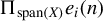 belongs to
$\mathfrak {M}_{0}^{lin}$
 . Again using Part 1, we arrive at
$i\in \mathcal {I}_{\#}$
 . That
$\mathcal {I}_{\#}$
 is a proper subset of
$\{1,\ldots ,n\}$
 follows since
$R\neq 0$
 .
Remark A.3. (i) Example A.1 below and the example discussed toward the end of Remark A.1(iv) show that the first two inclusions in Part 3 of the above lemma can be strict inclusions.
(ii) Inspection of the proof shows that Lemma A.4 actually also holds if, in the notation of Pötscher and Preinerstorfer (Reference Pötscher and Preinerstorfer2025), we have
$q\geq 1$
 , that is, if a collection of q restrictions is tested simultaneously.
The subsequent examples show that condition (7) can be stronger than condition (10), another such example being Example C.1 in Appendix C.1 of Pötscher and Preinerstorfer (Reference Pötscher and Preinerstorfer2025). We provide four different examples to illustrate that this can happen in a variety of different situations (e.g., independently of whether standard basis vectors belong to
$ \mathrm {span}(X)$
 or not, etc.). We also compute the set
$\mathsf {B}$
 in the examples below and illustrate the results in Lemma A.1.
Example A.1. Suppose
$k=2$
 ,
$n=4$
 , and X has
$(1,1,1,1)^{\prime }$
 as its first column and
$(1,-1,1,-1)^{\prime }$
 as its second column. Define the
$1\times k$
 vector
$R=(1,1)$
 . Then
$\mathrm {rank}(X)=k=2$
 holds, and
$ e_{j}(4)\notin \mathrm {span}(X)$
 for every
$j=1,\ldots ,4$
 , as is easily checked; in particular, Assumption 1 is thus satisfied, and
$ I_{1}(\mathfrak {M}_{0}^{lin})=\{1,\ldots ,4\}$
 . Furthermore,
$R(X^{\prime }X)^{-1}x_{i\cdot }^{\prime }\neq 0$
 for
$i=1,3,$
 whereas
$R(X^{\prime }X)^{-1}x_{i\cdot }^{\prime }=0$
 for
$i=2,4$
 . That is,
$\mathcal {I} _{\#}=\{2,4\} $
 . Now,
$y\in \mathsf {B}$
 (i.e.,
$B(y)=0$
 ) is easily seen to be equivalent to
$\hat {u}_{1}(y)=\hat {u}_{3}(y)=0$
 , which in turn is equivalent to
$y_{1}=y_{3}$
 . In particular,
$e_{2}(4)$
 and
$e_{4}(4)$
 belong to
$\mathsf {B}$
 , but do not belong to
$\mathrm {span}(X)$
 , while
$e_{1}(4)$
 and
$e_{3}(4)$
 do not belong to
$\mathsf {B}$
 . The space
$\{\hat {u}(y):y\in \mathsf {B}\}$
 in the orthogonal sum representation
$\mathsf {B}=\mathrm {span} (X)\oplus \{\hat {u}(y):y\in \mathsf {B}\}$
 is here given by
$\mathrm {span} ((0,1,0,-1)^{\prime })$
 as is not difficult to see. Note that, while
$ e_{2}(4)$
 and
$e_{4}(4)$
 belong to
$\mathsf {B}$
 (and trivially also to
$ \mathrm {span}(e_{i}(4):i\in \mathcal {I}_{\#})$
 ), they are not orthogonal to
$\mathrm {span}(X)$
 , and do not belong to
$\mathrm {span}((0,1,0,-1)^{\prime })$
 (which is a subset of
$\mathrm {span}(e_{i}(4):i\in \mathcal {I}_{\#})$
 ). Furthermore, since
$I_{1}(\mathfrak {M}_{0}^{lin})=\{1,\ldots ,4\}$
 , condition (10) is satisfied, while condition (7) is not. Theorem 2.1 does not allow one to draw a conclusion about size controllability of
$T_{Het}$
 in this example, while Theorem 2.2 shows that
$T_{Het}$
 is size controllable.
Example A.2. Suppose
$k=3$
 ,
$n=5$
 , and X has
$(1,1,1,1,0)^{\prime }$
 as its first column,
$(1,-1,1,-1,0)^{\prime }$
 as its second column, and
$ (0,0,0,0,2)^{\prime }$
 as its last column. Define the
$1\times k$
 vector
$ R=(1,1,r_{3})$
 . Then
$\mathrm {rank}(X)=k=3$
 holds, and
$e_{j}(5)\notin \mathrm {span}(X)$
 for every
$j=1,\ldots ,4$
 , but
$e_{5}(5)\in \mathrm {span} (X)$
 . Assumption 1 is satisfied as can be easily checked. Furthermore,
$R(X^{\prime }X)^{-1}x_{i\cdot }^{\prime }\neq 0$
 for
$i=1,3$
 , whereas
$R(X^{\prime }X)^{-1}x_{i\cdot }^{\prime }=0$
 for
$i=2,4$
 ; and
$ R(X^{\prime }X)^{-1}x_{5\cdot }^{\prime }=r_{3}/2$
 . Hence,
$\mathcal {I} _{\#}=\{2,4\}$
 in case
$r_{3}\neq 0$
 , and
$\mathcal {I}_{\#}=\{2,4,5\}$
 otherwise. Now,
$y\in \mathsf {B}$
 (i.e.,
$B(y)=0$
 ) is easily seen to be equivalent to
$\hat {u}_{1}(y)=\hat {u}_{3}(y)=0$
 , which in turn is equivalent to
$y_{1}=y_{3}$
 . In particular,
$e_{2}(5)$
 and
$e_{4}(5)$
 belong to
$ \mathsf {B}$
 , but do not belong to
$\mathrm {span}(X)$
 , while
$e_{5}(5)\in \mathrm {span}(X)\subseteq \mathsf {B}$
 ; and
$e_{1}(5)$
 and
$e_{3}(5)$
 do not belong to
$\mathsf {B}$
 . The space
$\{\hat {u}(y):y\in \mathsf {B}\}$
 in the orthogonal sum representation
$\mathsf {B}=\mathrm {span}(X)\oplus \{\hat {u} (y):y\in \mathsf {B}\}$
 is here given by
$\mathrm {span}((0,1,0,-1,0)^{\prime })$
 as is not difficult to see. Note that, while
$e_{2}(5)$
 and
$e_{4}(5)$
 belong to
$\mathsf {B}$
 (and trivially also to
$\mathrm {span}(e_{i}(5):i\in \mathcal {I}_{\#})$
 ), they are not orthogonal to
$\mathrm {span}(X)$
 , and do not belong to
$\mathrm {span}((0,1,0,-1,0)^{\prime })$
 (which is a subset of
$\mathrm {span}(e_{i}(5):i\in \mathcal {I}_{\#})$
 ). Note that
$I_{1}( \mathfrak {M}_{0}^{lin})=\{1,\ldots ,4\}$
 in case
$r_{3}=0$
 , while
$I_{1}( \mathfrak {M}_{0}^{lin})=\{1,\ldots ,5\}$
 otherwise. In particular, in case
$ r_{3}=0$
 , condition (10) is satisfied, while condition (7) is not; hence, in this case, Theorem 2.1 does not allow one to draw a conclusion about size controllability of
$T_{Het}$
 , while Theorem 2.2 shows that
$ T_{Het}$
 is size controllable. In case
$r_{3}\neq 0$
 , both conditions (7) and (10) are violated, and both theorems show that the test based on
$T_{Het}$
 has size
$1$
 regardless of the choice of critical value.
Example A.3. Suppose
$k=2$
 ,
$n=5$
 , and X has
$(1,1,1,1,0)^{\prime }$
 as its first column and
$(1,-1,1,-1,0)^{\prime }$
 as its second column. Define the
$1\times k$
 vector
$R=(1,0)$
 . Then
$\mathrm {rank}(X)=k=2$
 holds, and
$e_{j}(5)\notin \mathrm {span}(X)$
 for every
$j=1,\ldots ,5$
 , as is easily checked; in particular, Assumption 1 is thus satisfied, and
$I_{1}(\mathfrak {M}_{0}^{lin})=\{1,\ldots ,5\}$
 . Furthermore,
$ R(X^{\prime }X)^{-1}x_{i\cdot }^{\prime }\neq 0$
 for
$i=1,\ldots ,4,$
 whereas
$R(X^{\prime }X)^{-1}x_{5\cdot }^{\prime }=0$
 . That is,
$\mathcal {I}_{\#}=\{5\}$
 . Now,
$y\in \mathsf {B}$
 (i.e.,
$B(y)=0$
 ) is easily seen to be equivalent to
$\hat {u}_{1}(y)=\hat {u}_{2}(y)=\hat {u}_{3}(y)=\hat {u}_{4}(y)=0$
 , which in turn is equivalent to
$y_{1}=y_{3}$
 and
$y_{2}=y_{4}$
 . In particular,
$ e_{5}(5)$
 belongs to
$\mathsf {B}$
 , but does not belong to
$\mathrm {span}(X)$
 , in fact is orthogonal to
$\mathrm {span}(X)$
 , while
$e_{j}(5)\notin \mathsf {B}$
 for
$j=1,\ldots ,4$
 . The space
$\{\hat {u}(y):y\in \mathsf {B}\}$
 in the orthogonal sum representation
$\mathsf {B}=\mathrm {span}(X)\oplus \{ \hat {u}(y):y\in \mathsf {B}\}$
 is here given by
$\mathrm {span}(e_{5}(5))$
 as is not difficult to see. Furthermore, in this example, condition (10) is satisfied, while condition (7) is not. Theorem 2.1 does not allow one to draw a conclusion about size controllability of
$T_{Het}$
 in this example, while Theorem 2.2 shows that
$T_{Het}$
 is size controllable.
Example A.4. Suppose
$k=3$
 ,
$n=6$
 , and X has
$(1,1,1,1,0,0)^{ \prime }$
 as its first column,
$(1,-1,1,-1,0,0)^{\prime }$
 as its second column, and
$(0,0,0,0,0,2)^{\prime }$
 as its third column. Define the
$ 1\times k$
 vector
$R=(1,0,r_{3})$
 . Then
$\mathrm {rank}(X)=k=3$
 holds, and
$ e_{j}(6)\notin \mathrm {span}(X)$
 for every
$j=1,\ldots ,5$
 , but
$ e_{6}(6)\in \mathrm {span}(X)$
 . Assumption 1 is satisfied as can be easily checked. Furthermore,
$R(X^{\prime }X)^{-1}x_{i\cdot }^{\prime }\neq 0$
 for
$i=1,\ldots ,4,$
 whereas
$R(X^{\prime }X)^{-1}x_{5\cdot }^{\prime }=0$
 and
$R(X^{\prime }X)^{-1}x_{6\cdot }^{\prime }=r_{3}/2$
 . Hence,
$\mathcal {I}_{\#}=\{5\}$
 in case
$r_{3}\neq 0,$
 and
$\mathcal {I} _{\#}=\{5,6\}$
 otherwise. Now,
$y\in \mathsf {B}$
 (i.e.,
$B(y)=0$
 ) is easily seen to be equivalent to
$\hat {u}_{1}(y)=\hat {u}_{2}(y)=\hat {u}_{3}(y)=\hat {u }_{4}(y)=0$
 , which in turn is equivalent to
$y_{1}=y_{3}$
 and
$y_{2}=y_{4}$
 . In particular,
$e_{5}(6)$
 belongs to
$\mathsf {B}$
 , but does not belong to
$ \mathrm {span}(X)$
 , in fact is orthogonal to
$\mathrm {span}(X)$
 , while
$ e_{6}(6)\in \mathrm {span}(X)\subseteq \mathsf {B}$
 ; and
$e_{j}(6)\notin \mathsf {B}$
 for
$j=1,\ldots ,4$
 . The space
$\{\hat {u}(y):y\in \mathsf {B}\}$
 in the orthogonal sum representation
$\mathsf {B}=\mathrm {span}(X)\oplus \{ \hat {u}(y):y\in \mathsf {B}\}$
 is here given by
$\mathrm {span}(e_{5}(6))$
 as is not difficult to see. Note that
$I_{1}(\mathfrak {M}_{0}^{lin})=\{1,\ldots ,5\}$
 in case
$r_{3}=0$
 , while
$I_{1}(\mathfrak {M}_{0}^{lin})=\{1,\ldots ,6\} $
 otherwise. In particular, in case
$r_{3}=0$
 , condition (10) is satisfied, while condition (7) is not; hence, in this case, Theorem 2.1 does not allow one to draw a conclusion about size controllability of
$T_{Het}$
 , while Theorem 2.2 shows that
$T_{Het}$
 is size controllable. In case
$r_{3}\neq 0$
 , both conditions (7) and (10) are violated, and both theorems show that the test based on
$T_{Het}$
 has size
$ 1 $
 regardless of the choice of critical value.
Remark A.4. Many more examples can be generated from Examples A.1–A.4 via the transformation
$X^{\ast }=XA$
 and
$R^{\ast }=RA,$
 where A is a nonsingular
$k\times k$
 matrix. These new examples exhibit the same features as Examples A.1–A.4, respectively. In particular, one can generate examples that have
$R^{\ast }=(1,0\ldots ,0)$
 .
B PROOF OF THEOREM 2.2
To prove Theorem 2.2, we follow the strategy used to establish Theorem 5.1 in Pötscher and Preinerstorfer (Reference Pötscher and Preinerstorfer2025) and first provide a result for a class of heteroskedasticity models that includes
$\mathfrak {C}_{Het}$
 as a special case, and which is of some independent interest. The heteroskedasticity models we consider here are defined as follows (cf. Appendix A of Pötscher and Preinerstorfer, Reference Pötscher and Preinerstorfer2025, for more discussion): Let
$m\in \mathbb {N}$
 , and let
$n_{j}\in \mathbb {N}$
 for
$j=1,\ldots ,m$
 satisfy
$\sum _{j=1}^{m}n_{j}=n$
 . Set
$ n_{j}^{+}=\sum _{l=1}^{j}n_{l}$
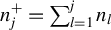 and define

with the convention that
$n_{0}^{+}=0$
 . In the special case where
$m=n$
 and
$ n_{1}=n_{2}=\cdots =n_{m}=1,$
 we have
$\mathfrak {C}_{(n_{1},\ldots ,n_{m})}= \mathfrak {C}_{Het}$
 . We use
$\lambda _{\mathbb {R}^{n}}$
 to denote Lebesgue measure on
$\mathbb {R}^{n}$
 , and
$\lambda _{\mathcal {A}}$
 to denote Lebesgue measure on a (nonempty) affine space
$\mathcal {A}$
 (but viewed as a measure on the Borel sets of
$\mathbb {R}^{n}$
 ), with zero-dimensional Lebesgue measure interpreted as point mass. We start with a lemma and note that it does not make use of Assumption 1. Recall that by definition
$\mathcal {L}_{\#}=\mathrm {span}(\mathfrak {M}_{0}^{lin}\cup \mathcal {V}_{\#})$
 , and that we only consider testing a single restriction in the present article.
Lemma B.1. Let
$m\in \mathbb {N}$
 , and let
$n_{j}\in \mathbb {N}$
 for
$j=1,\ldots ,m$
 satisfy
$\sum _{j=1}^{m}n_{j}=n$
 . Then:
(a) The condition

is equivalent to the condition

(It is understood here that condition (B.3) is satisfied if no j with
$\emptyset \neq (n_{j-1}^{+},n_{j}^{+}]\cap I_{1}( \mathcal {L}_{\#})\subseteq \mathcal {I}_{\#}^{c}$
 exists.)
(b) In the special case where
$m=n$
 and
$n_{1}=n_{2}=\cdots =n_{m}=1$
 , (B.3) (as well as (B.2)) is equivalent to (10).
Proof. (a) Recall from the proof of Part 1 of Lemma A.2 that
$\mathcal {L}_{\#}=\mathrm {span}(\mathfrak {M} _{0}^{lin}\cup \mathcal {V}_{\#})\subseteqq \mathsf {B}$
 . Therefore,
$ e_{i}(n)\notin \mathsf {B}$
 is possible only if
$i\in I_{1}(\mathcal {L}_{\#})$
 . Hence, in view of invariance of
$\mathsf {B}$
 w.r.t. addition of elements of
$\mathsf {B}$
 (Lemma A.2), the condition in (B.2) is equivalent to

For
$i\in \mathcal {I}_{\#}$
 , the condition
$e_{i}(n)\in \mathsf {B}$
 implies
$ e_{i}(n)\in \mathcal {V}_{\#}\subseteq \mathcal {L}_{\#}$
 , so that
$i\notin I_{1}(\mathcal {L}_{\#})$
 . In other words,
$i\in I_{1}(\mathcal {L}_{\#})\cap \mathcal {I}_{\#}$
 implies
$e_{i}(n)\notin \mathsf {B}$
 . This shows that for any j with the property that
$(n_{j-1}^{+},n_{j}^{+}]\cap I_{1}(\mathcal {L} _{\#})$
 contains an element
$i\in \mathcal {I}_{\#}$
 , the non-inclusion relation in (B.4) is automatically satisfied. Hence, (B.4) is equivalent to

with the understanding that this condition is satisfied if no j with
$ \emptyset \neq (n_{j-1}^{+},n_{j}^{+}]\cap I_{1}(\mathcal {L}_{\#})\subseteq \mathcal {I}_{\#}^{c}$
 exists. Since
$\mathsf {B}$
 as well as
$\mathrm {span} (X)$
 are a linear spaces, Part 4 of Lemma A.1 shows that (B.5) is equivalent to the statement in (B.3).
(b) In the special case considered here (B.3) simplifies to

with the understanding as in (B.3) that this condition is satisfied if
$I_{1}(\mathcal {L}_{\#})\cap \mathcal {I}_{\#}^{c}$
 is empty. Since
$I_{1}(\mathcal {L}_{\#})\cap \mathcal {I}_{\#}^{c}=\mathcal {I} _{\#}^{c}\neq \emptyset $
 by Part 3 of Lemma A.4, the index set in (B.6) is actually nonempty, and furthermore (B.6) is equivalent to

Because of
$\mathcal {I}_{\#}^{c}\subseteq I_{1}(\mathfrak {M}_{0}^{lin})$
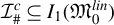 (Lemma A.4), the statement in (B.7) is implied by that in (10). To show that (B.7) implies (10), suppose (10) is violated, that is, there exists an
$i\in I_{1}(\mathfrak {M}_{0}^{lin})$
 such that
$ e_{i}(n)\in \mathrm {span}(X)$
 . It then follows that
$R\hat {\beta } (e_{i}(n))\neq 0$
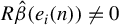 must hold. Since
$R\hat {\beta }(e_{i}(n))=R(X^{\prime }X)^{-1}x_{i\cdot }^{\prime }$
 , we conclude
$i\in \mathcal {I}_{\#}^{c}$
 . Hence, (B.7) must also be violated, a contradiction.
Parts 1 and 2 of the following statement provide—in the context of testing a single restriction—a version of Theorem A.1(b) and the corresponding part of Theorem A.1(c) in Pötscher and Preinerstorfer (Reference Pötscher and Preinerstorfer2025), while Part 3 corresponds to the generalization of Proposition 5.5(b) mentioned after Theorem A.1 in Pötscher and Preinerstorfer (Reference Pötscher and Preinerstorfer2025). Part 4 of the subsequent theorem is a version of Proposition A.2(b) in Pötscher and Preinerstorfer (Reference Pötscher and Preinerstorfer2025), and together with Part 1 shows that, under Assumption 1, the condition in (B.2), or equivalently (B.3), is necessary and sufficient for the existence of a (finite) critical value that controls the size of
$T_{Het}$
 over the heteroskedasticity model
$\mathfrak {C}_{(n_{1},\ldots ,n_{m})}$
 when testing

Theorem B.2. Let
$m\in \mathbb {N}$
 , let
$n_{j}\in \mathbb {N}$
 for
$ j=1,\ldots ,m$
 satisfy
$\sum _{j=1}^{m}n_{j}=n$
 , and suppose Assumption 1 is satisfied. Then the following statements hold:
-
1. For every $0<\alpha <1,$
there exists a real number
$C(\alpha )$
such that (B.8) $$ \begin{align} \sup_{\mu _{0}\in \mathfrak{M}_{0}}\sup_{0<\sigma ^{2}<\infty }\sup_{\Sigma \in \mathfrak{C}_{(n_{1},\ldots ,n_{m})}}P_{\mu _{0},\sigma ^{2}\Sigma }(T_{Het}\geq C(\alpha ))\leq \alpha \end{align} $$holds, provided that (B.2) (or equivalently (B.3)) holds. Furthermore, under condition (B.2) (or equivalently (B.3)), even equality can be achieved in (B.8) by a proper choice of $C(\alpha )$
, provided
$\alpha \in (0,\alpha ^{\ast }]\cap (0,1)$
holds, where $$ \begin{align*} \alpha ^{\ast }=\sup_{C\in (C^{\ast },\infty )}\sup_{\Sigma \in \mathfrak{C} _{(n_{1},\ldots ,n_{m})}}P_{\mu _{0},\Sigma }(T_{Het}\geq C) \end{align*} $$is positive and where $C^{\ast }$
is defined as in Lemma 5.11 of Pötscher and Preinerstorfer (Reference Pötscher and Preinerstorfer2018) with
$\mathfrak {C}=\mathfrak {C}_{(n_{1},\ldots ,n_{m})}$
,
$T=T_{Het}$
,
$ N^{\dagger }=\mathsf {B}$
,
$\mathcal {L}=\mathcal {L}_{\#}$
, and
$q=1$
(with neither
$\alpha ^{\ast }$
nor
$C^{\ast }$
depending on the choice of
$\mu _{0}\in \mathfrak {M}_{0}$
).
-
2. Suppose (B.2) (or equivalently (B.3)) is satisfied. Then a smallest critical value, denoted by $C_{\Diamond }(\alpha )$
, satisfying (B.8) exists for every
$0<\alpha <1$
. And
$C_{\Diamond }(\alpha )$
is also the smallest among the critical values leading to equality in (B.8) whenever such critical values exist.Footnote
22
-
3. Suppose (B.2) (or equivalently (B.3)) is satisfied. Then any $C(\alpha )$
satisfying (B.8) necessarily has to satisfy
$C(\alpha )\geq C^{\ast }$
. In fact, for any
$C<C^{\ast }$
, we have
$\sup _{\Sigma \in \mathfrak {C}_{(n_{1},\ldots ,n_{m})}}P_{\mu _{0},\sigma ^{2}\Sigma }(T_{Het}\geq C)=1$
for every
$\mu _{0}\in \mathfrak {M}_{0}$
and every
$ \sigma ^{2}\in (0,\infty )$
. -
4. If (B.2) (or equivalently (B.3)) is violated, then $\sup _{\Sigma \in \mathfrak {C} _{(n_{1},\ldots ,n_{m})}}P_{\mu _{0},\sigma ^{2}\Sigma }(T_{Het}\geq C)=1$
for every choice of critical value C, every
$\mu _{0}\in \mathfrak {M }_{0}$
, and every
$\sigma ^{2}\in (0,\infty )$
(implying that size equals
$1$
for every C).Footnote
23














The following proof adapts the proof of Theorem A.1 in Pötscher and Preinerstorfer (Reference Pötscher and Preinerstorfer2025).
Proof of Theorem B.2
We first prove Part 1. We apply Part A of Proposition 5.12 of Pötscher and Preinerstorfer (Reference Pötscher and Preinerstorfer2018) with
$\mathfrak {C}=\mathfrak {C} _{(n_{1},\ldots ,n_{m})}$
 ,
$T=T_{Het}$
 ,
$\mathcal {L}=\mathcal {L}_{\#}$
 , and
$ \mathcal {V}=\mathcal {V}_{\#}$
 (and
$q=1$
 ). First, note that
$\dim (\mathcal {L }_{\#})<n-1<n$
 because of Lemma A.3. Second, under Assumption 1,
$T_{Het}$
 is a non-sphericity corrected F-type test statistic with
$N^{\ast }=\mathsf {B}$
 , which is a closed
$\lambda _{\mathbb {R}^{n}}$
 -null set (see Remarks 3.2 and C.1 as well as Lemma 3.1 in Pötscher and Preinerstorfer, Reference Pötscher and Preinerstorfer2025); in particular,
$T_{Het}$
 as well as
$\mathsf {B}$
 are invariant w.r.t. the group
$G(\mathfrak {M}_{0})$
 . Furthermore,
$T_{Het}$
 as well as
$\mathsf {B}$
 are invariant w.r.t. addition of elements of
$\mathcal {V}_{\#}$
 by Lemma A.2. Hence, the general assumptions on
$T=T_{Het}$
 , on
$N^{\dagger }=N^{\ast }=\mathsf {B}$
 , on
$\mathcal {V}=\mathcal {V}_{\#}$
 , as well as on
$ \mathcal {L}=\mathcal {L}_{\#}$
 in Proposition 5.12 of Pötscher and Preinerstorfer (Reference Pötscher and Preinerstorfer2018) are satisfied in view of Part 1 of Lemma 5.16 in the same reference.
Next, observe that condition (B.2) is equivalent to

for every
$j=1,\ldots ,m$
 , such that
$(n_{j-1}^{+},n_{j}^{+}]\cap I_{1}( \mathcal {L}_{\#})\neq \emptyset $
 , since
$\Pi _{\mathcal {L}_{\#}^{\bot }}e_{i}(n)$
 and
$e_{i}(n)$
 differ only by an element of
$\mathcal {L}_{\#}$
 and since
$\mathsf {B}+\mathcal {L}_{\#}=\mathsf {B}$
 (which follows from Part 1 of Lemma A.2). In view of Proposition B.2 in Appendix B of Pötscher and Preinerstorfer (Reference Pötscher and Preinerstorfer2025), this implies that any
$\mathcal {S}\in \mathbb {J}(\mathcal {L} _{\#},\mathfrak {C}_{(n_{1},\ldots ,n_{m})})$
 is not contained in
$\mathsf {B}$
 , and thus not in
$N^{\dagger }$
 . Using
$\mathfrak {M}_{0}\subseteq \mathrm {span }(X)$
 and
$\mathsf {B}+\mathrm {span}(X)=\mathsf {B}$
 (by Lemma 3.1(e) in Pötscher and Preinerstorfer, Reference Pötscher and Preinerstorfer2025), it follows that
$\mu _{0}+\mathcal {S}\nsubseteqq \mathsf {B}=N^{\dagger }$
 for every
$\mu _{0}\in \mathfrak {M}_{0}$
 . Since
$\mu _{0}+\mathcal {S}$
 is a (nonempty) affine space and
$N^{\dagger }=\mathsf {B}$
 is a linear space (recall that R is
$1\times k$
 ), we may conclude (cf. Corollary 5.6 in Pötscher and Preinerstorfer, Reference Pötscher and Preinerstorfer2018 and its proof) that
$\lambda _{\mu _{0}+\mathcal {S}}(N^{\dagger })=0$
 for every
$\mathcal {S}\in \mathbb {J}(\mathcal {L}_{\#},\mathfrak {C} _{(n_{1},\ldots ,n_{m})})$
 and every
$\mu _{0}\in \mathfrak {M}_{0}$
 . This completes the verification of the assumptions of Proposition 5.12 in Pötscher and Preinerstorfer (Reference Pötscher and Preinerstorfer2018) that are not specific to Part A (or Part B) of this proposition.
We next verify the assumptions specific to Part A of this proposition: Assumption (a) is satisfied (even for every
$C\in \mathbb {R}$
 ) as a consequence of Part 2 of Lemma 5.16 in Pötscher and Preinerstorfer (Reference Pötscher and Preinerstorfer2018) and of Remark C.1(i) in Appendix C of Pötscher and Preinerstorfer (Reference Pötscher and Preinerstorfer2025). And Assumption (b) in Part A follows from Lemma 5.19 of Pötscher and Preinerstorfer (Reference Pötscher and Preinerstorfer2018), since
$T_{Het}$
 results as a special case of the test statistics
$T_{GQ}$
 defined in Section 3.4 of Pötscher and Preinerstorfer (Reference Pötscher and Preinerstorfer2018) upon choosing
$ \mathcal {W}_{n}^{\ast }=n^{-1}\mathrm {diag}(d_{1},\ldots ,d_{n})$
 . Part A of Proposition 5.12 of Pötscher and Preinerstorfer (Reference Pötscher and Preinerstorfer2018) now immediately delivers claim (B.8), since
$C^{\ast }<\infty $
 as noted in that proposition. That
$C^{\ast }$
 and
$\alpha ^{\ast }$
 do not depend on the choice of
$\mu _{0}\in \mathfrak {M}_{0}$
 is an immediate consequence of
$G( \mathfrak {M}_{0})$
 -invariance of
$T_{Het}$
 (cf. Remark 3.2 in Pötscher and Preinerstorfer, Reference Pötscher and Preinerstorfer2025). Also note that
$\alpha ^{\ast }$
 as defined in the theorem coincides with
$ \alpha ^{\ast }$
 as defined in Proposition 5.12 of Pötscher and Preinerstorfer (Reference Pötscher and Preinerstorfer2018) in view of
$G( \mathfrak {M}_{0})$
 -invariance of
$T_{Het}$
 . Positivity of
$\alpha ^{\ast }$
 then follows from Part 5 of Lemma 5.15 in Preinerstorfer and Pötscher (Reference Preinerstorfer and Pötscher2016) in view of Remark C.1(i) in Appendix C of Pötscher and Preinerstorfer (Reference Pötscher and Preinerstorfer2025), noting that
$\lambda _{\mathbb {R}^{n}}$
 and
$P_{\mu _{0},\Sigma }$
 are equivalent measures (since
$\Sigma \in \mathfrak {C}_{Het}$
 is positive definite); cf. Remark 5.13(vi) in Pötscher and Preinerstorfer (Reference Pötscher and Preinerstorfer2018). In case
$\alpha <\alpha ^{\ast }$
 , the remaining claim in Part 1 of the present theorem, namely, that equality can be achieved in (B.8), follows from the definition of
$C^{\ast }$
 in Lemma 5.11 of Pötscher and Preinerstorfer (Reference Pötscher and Preinerstorfer2018) and from Part A.2 of Proposition 5.12 of Pötscher and Preinerstorfer (Reference Pötscher and Preinerstorfer2018) (and the observation immediately following that proposition allowing one to drop the suprema w.r.t.
$\mu _{0}$
 and
$\sigma ^{2}$
 , and to set
$\sigma ^{2}=1$
 ); in case
$\alpha =\alpha ^{\ast }<1$
 , it follows from Remark 5.13(i) and (ii) in Pötscher and Preinerstorfer (Reference Pötscher and Preinerstorfer2018) using Lemma 5.16 in the same reference.
The claim in Part 2 follows from Remark 5.10 and Lemma 5.16 in Pötscher and Preinerstorfer (Reference Pötscher and Preinerstorfer2018) combined with Remark C.1(i) in Appendix C of Pötscher and Preinerstorfer (Reference Pötscher and Preinerstorfer2025); cf. also Appendix A.3 in Pötscher and Preinerstorfer (Reference Pötscher and Preinerstorfer2025).
Part 3 follows from Part A.1 of Proposition 5.12 of Pötscher and Preinerstorfer (Reference Pötscher and Preinerstorfer2018) and the sentence following this proposition. Note that the assumptions of this proposition have been verified in the proof of Part 1 above.
Part 4 follows from Part 3 of Corollary 5.17 in Preinerstorfer and Pötscher (Reference Preinerstorfer and Pötscher2016): As shown in Remark C.1 in Appendix C of Pötscher and Preinerstorfer (Reference Pötscher and Preinerstorfer2025),
$T_{Het}$
 satisfies the assumptions of this corollary (with
$\check {\beta }=\hat {\beta }$
 ,
$\check {\Omega }=\hat { \Omega }_{Het}$
 ,
$N=\emptyset $
 , and
$N^{\ast }=\mathsf {B}$
 ). Suppose that ( B.3) is violated and set
$\mathcal {Z}=\mathrm {span} (\{e_{i}(n):i\in (n_{j-1}^{+},n_{j}^{+}]\})$
 , where j is such that
$ \emptyset \neq (n_{j-1}^{+},n_{j}^{+}]\cap I_{1}(\mathcal {L}_{\#})\subseteq \mathcal {I}_{\#}^{c}$
 and

Since
$e_{i}(n)\in \mathcal {L}_{\#}$
 for every
$i\in I_{0}(\mathcal {L}_{\#})$
 , it hence follows from (B.9) that
$\mathcal {Z}\subseteq \mathrm {span }(\mathrm {span}(X)\cup \mathcal {L}_{\#})\subseteq \mathsf {B}$
 , recalling that
$\mathrm {span}(X)\subseteq \mathsf {B}$
 , that
$\mathcal {L} _{\#}\subseteq \mathsf {B}$
 (cf. the proof of Part 1 of Lemma A.2), and that
$\mathsf {B}$
 is a linear space (recall that R is
$1\times k$
 ). Note that
$\mathcal {Z}$
 is not contained in
$\mathfrak {M} _{0}^{lin}$
 because
$\emptyset \neq (n_{j-1}^{+},n_{j}^{+}]\cap I_{1}( \mathcal {L}_{\#})$
 but
$\mathfrak {M}_{0}^{lin}\subseteq \mathcal {L}_{\#}$
 . Observe that
$\mathcal {Z}$
 is a concentration space of
$\mathfrak {C} _{(n_{1},\ldots ,n_{m})}$
 in view of Remark B.4 in Appendix B of Pötscher and Preinerstorfer (Reference Pötscher and Preinerstorfer2025) (note that
$\mathrm {card}((n_{j-1}^{+},n_{j}^{+}])<n$
 must hold in view of
$ \mathcal {Z}\subseteq \mathsf {B}$
 and
$\mathsf {B}$
 being a proper subspace of
$\mathbb {R}^{n}$
 by Lemma 3.1 in Pötscher and Preinerstorfer (Reference Pötscher and Preinerstorfer2025) in conjunction with Assumption 1, while
$0<\mathrm {card}((n_{j-1}^{+},n_{j}^{+}])$
 is obvious). The nonnegative definiteness assumption on
$\check {\Omega }=\hat { \Omega }_{Het}$
 in Part 3 of Corollary 5.17 in Preinerstorfer and Pötscher (Reference Preinerstorfer and Pötscher2016) is satisfied (cf. Lemma 3.1 in Pötscher and Preinerstorfer, Reference Pötscher and Preinerstorfer2025). Obviously,
$\check {\Omega }(z)=0$
 holds for every
$z\in \mathcal {Z}$
 as a consequence of Part (b) of Lemma 3.1 in Pötscher and Preinerstorfer (Reference Pötscher and Preinerstorfer2025) since
$\mathcal {Z}\subseteq \mathsf {B}$
 (as just shown) and since
$ \check {\Omega }(z)$
 is
$1\times 1$
 . It remains to establish that
$R\hat {\beta } (z)\neq 0$
 holds
$\lambda _{\mathcal {Z}}$
 -everywhere: we recall that
$ \emptyset \neq (n_{j-1}^{+},n_{j}^{+}]\cap I_{1}(\mathcal {L}_{\#})\subseteq \mathcal {I}_{\#}^{c}$
 and pick an element i, say, of
$ (n_{j-1}^{+},n_{j}^{+}]\cap I_{1}(\mathcal {L}_{\#})$
 . Then
$e_{i}(n)\in \mathcal {Z}$
 and
$i\in \mathcal {I}_{\#}^{c}$
 , and from the definition of
$ \mathcal {I}_{\#}^{c}$
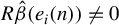
 , we conclude that
$R\hat {\beta }(e_{i}(n))\neq 0$
 . It follows that the linear space
$\mathcal {Z}$
 is not a subspace of the kernel of
$R\hat {\beta }$
 so that
$R\hat {\beta }(z)\neq 0$
 holds
$\lambda _{\mathcal {Z }}$
 -everywhere. Part 3 of Corollary 5.17 in Preinerstorfer and Pötscher (Reference Preinerstorfer and Pötscher2016) then proves the claim for
$C>0$
 . A fortiori it then also holds for all real C.
We are now ready to prove Theorem 2.2. The proof follows the structure of the proof of Theorem 5.1 in Pötscher and Preinerstorfer (Reference Pötscher and Preinerstorfer2025).
Proof of Theorem 2.2
We apply Theorem B.2 with
$m=n$
 and
$n_{j}=1$
 for
$j=1,\ldots ,m$
 , observing that then
$\mathfrak { C}_{(n_{1},\ldots ,n_{m})}=\mathfrak {C}_{Het}$
 and that condition (10) is equivalent to (B.2) by Part (b) of Lemma B.1. This then establishes that (6) follows from (10). The remaining claim in Part 1 of Theorem 2.2 follows from Part 1 of Theorem B.2, if we can show that
$\alpha ^{\ast }$
 and
$C^{\ast }$
 given in Theorem B.2 can be written as claimed in Theorem 2.2. To show this, we proceed as follows: Choose an element
$\mu _{0}$
 of
$\mathfrak {M}_{0}$
 . Observe that
$I_{1}(\mathcal {L}_{\#})\neq \emptyset $
 (since
$\dim (\mathcal {L}_{\#})<n-1<n$
 , cf. Lemma A.3), and that for every
$i\in I_{1}(\mathcal {L}_{\#}),$
 the linear space
$\mathcal {S} _{i}=\mathrm {span}(\Pi _{\mathcal {L}_{\#}^{\bot }}e_{i}(n))$
 is one-dimensional (since
$\mathcal {S}_{i}=\{0\}$
 is impossible in view of
$i\in I_{1}(\mathcal {L}_{\#})$
 ) and belongs to
$\mathbb {J}(\mathcal {L}_{\#}, \mathfrak {C}_{Het})$
 in view of Proposition B.1 in Appendix B of Pötscher and Preinerstorfer (Reference Pötscher and Preinerstorfer2025) together with
$\mathrm {dim}(\mathcal {L}_{\#})<n-1$
 . Since
$T_{Het}$
 is
$G( \mathfrak {M}_{0})$
 -invariant (Remark C.1(i) in Appendix C of Pötscher and Preinerstorfer, Reference Pötscher and Preinerstorfer2025), it follows that
$T_{Het}$
 is constant on
$(\mu _{0}+\mathcal {S} _{i})\backslash \left \{ \mu _{0}\right \} $
 (cf. the beginning of the proof of Lemma 5.11 in Pötscher and Preinerstorfer, Reference Pötscher and Preinerstorfer2018). Hence,
$\mathcal {S}_{i}$
 belongs to
$\mathbb {H}$
 (defined in Lemma 5.11 in Pötscher and Preinerstorfer, Reference Pötscher and Preinerstorfer2018) and consequently for
$C^{\ast }$
 as defined in that lemma

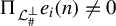
must hold (recall that
$\Pi _{\mathcal {L}_{\#}^{\bot }}e_{i}(n)\neq 0$
 ). To prove the opposite inequality, let
$\mathcal {S}$
 be an arbitrary element of
$ \mathbb {H}$
 , that is,
$\mathcal {S}\in \mathbb {J}(\mathcal {L}_{\#},\mathfrak {C} _{Het})$
 and
$T_{Het}$
 is
$\lambda _{\mu _{0}+\mathcal {S}}$
 -almost everywhere equal to a constant
$C(\mathcal {S})$
 , say. Then Proposition B.1 in Appendix B of Pötscher and Preinerstorfer (Reference Pötscher and Preinerstorfer2025) together with
$\mathrm {dim}(\mathcal {L} _{\#})<n-1$
 shows that
$\mathcal {S}_{i}\subseteq \mathcal {S}$
 holds for some
$i\in I_{1}(\mathcal {L}_{\#})$
 . By Remark B.1(iv) given below, the condition in (10) is equivalent to

Therefore, (10) implies that we have
$\mathcal {S} _{i}\nsubseteqq \mathsf {B}$
 since
$\Pi _{\mathcal {L}_{\#}^{\bot }}e_{i}(n)$
 and
$e_{i}(n)$
 differ only by an element of
$\mathcal {L}_{\#}$
 and since
$ \mathsf {B}+\mathcal {L}_{\#}=\mathsf {B}$
 (because of Part 1 of Lemma A.2). Thus,
$\mu _{0}+\mathcal {S}_{i}\nsubseteqq \mathsf {B}$
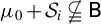 by the same argument as
$\mu _{0}\in \mathfrak {M}_{0}\subseteq \mathrm {span} (X) $
 and
$\mathsf {B}+\mathrm {span}(X)=\mathsf {B}$
 . We thus can find
$s\in \mathcal {S}_{i}$
 such that
$\mu _{0}+s\notin \mathsf {B}$
 . Note that
$s\neq 0$
 must hold, since
$\mu _{0}\in \mathfrak {M}_{0}\subseteq \mathrm {span} (X)\subseteq \mathsf {B}$
 . In particular,
$T_{Het}$
 is continuous at
$\mu _{0}+s$
 , since
$\mu _{0}+s\notin \mathsf {B}$
 . Now, for every open ball
$ A_{\varepsilon }$
 in
$\mathbb {R}^{n}$
 with center s and radius
$ \varepsilon>0,$
 we can find an element
$a_{\varepsilon }\in A_{\varepsilon }\cap \mathcal {S}$
 such that
$T_{Het}(\mu _{0}+a_{\varepsilon })=C(\mathcal {S })$
 . Since
$a_{\varepsilon }\rightarrow s$
 for
$\varepsilon \rightarrow 0$
 , it follows that
$C(\mathcal {S})=T_{Het}(\mu _{0}+s)$
 . Since
$s\neq 0$
 and since
$T_{Het}$
 is constant on
$(\mu _{0}+\mathcal {S}_{i})\backslash \left \{ \mu _{0}\right \} $
 as shown before, we can conclude that
$C(\mathcal {S} )=T_{Het}(\mu _{0}+s)=T_{Het}(\mu _{0}+\Pi _{\mathcal {L}_{\#}^{\bot }}e_{i}(n))$
 , where we recall that
$\Pi _{\mathcal {L}^{\bot }}e_{i}(n)\neq 0$
 . But this now, together with (B.10), implies

Using invariance of
$T_{Het}$
 w.r.t. addition of elements of
$\mathcal {L} _{\#}$
 (cf. Lemma A.2), we conclude that

Recall that
$I_{1}(\mathcal {L}_{\#})\subseteq I_{1}(\mathfrak {M}_{0}^{lin})$
 . For
$i\in I_{1}(\mathfrak {M}_{0}^{lin})\left \backslash I_{1}(\mathcal {L} _{\#}),\right. $
 we have
$i\in I_{0}(\mathcal {L}_{\#})$
 , and thus
$ e_{i}(n)\in \mathcal {L}_{\#}$
 . Since
$\mathcal {L}_{\#}\subseteq \mathsf {B}$
 ,
$e_{i}(n)\in \mathsf {B}$
 follows. Using Part 1 of Lemma A.2 and
$\mathfrak {M}_{0}\subseteq \mathsf {B}$
 , we conclude that
$\mu _{0}+e_{i}(n)\in \mathsf {B}$
 , and thus
$T_{Het}(\mu _{0}+e_{i}(n))=0$
 . Since
$T_{Het}$
 is always nonnegative and since
$I_{1}(\mathcal {L}_{\#})$
 is nonempty, we can write (B.11) equivalently as

The expression for
$\alpha ^{\ast }$
 given in the theorem now follows immediately from the expression for
$\alpha ^{\ast }$
 given in Part 1 of Theorem B.2.
Parts 2–4 now follow from the corresponding parts of Theorem B.2 in light of what has been shown above.
Remark B.1 (Equivalent forms of the size-control conditions)
(i) The proof of Lemma B.1 has shown that (B.2) is not only equivalent to (B.3), but also to (B.4) as well as to (B.5).
(ii) Non-inclusion statements of the form “
$\mathrm {span}\left ( \left \{ e_{i}(n):i\in J\right \} \right ) \nsubseteqq \mathsf {B}$
 ” (J an index set) appearing in (B.2), (B.4), and ( B.5) can equivalently be written as “
$e_{i}(n)\notin \mathsf {B}$
 for some
$i\in J$
 ” due to the fact that
$\mathsf {B}$
 is a linear space (as R is
$1\times k$
 ). Similarly, “
$\mathrm {span}\left ( \left \{ e_{i}(n):i\in J\right \} \right ) \nsubseteqq \mathrm {span}(X)$
 ” is equivalent to “
$e_{i}(n)\notin \mathrm {span}(X)$
 for some
$i\in J$
 .”
(iii) In the special case where
$m=n$
 and
$n_{1}=n_{2}=\cdots =n_{m}=1$
 , we learn from Lemma B.1 and its proof that (10) is equivalent to (B.6), as well as to (B.7). Since
$\mathcal {I}_{\#}^{c}\subseteq I_{1}( \mathcal {L}_{\#})\subseteq I_{1}(\mathfrak {M}_{0}^{lin})$
 by Part 3 of Lemma A.4, each one of (10), (B.6), and (B.7) is in turn equivalent to the condition

(As a point of interest, we note that conditions (10), (B.6), (B.7), and (B.12) are in fact equivalent also if, in the notation of Pötscher and Preinerstorfer, Reference Pötscher and Preinerstorfer2025, we have
$q\geq 1$
 , that is, if a collection of q restrictions is tested simultaneously. This can be seen by an inspection of the proofs of these equivalences. However, note that, in case
$q>1,$
 we have no result guaranteeing that these conditions are sufficient for size controllability of
$T_{Het}$
 .)
(iv) Specializing Part (a) of Lemma B.1 and its proof to the case
$n_{j}=1$
 for
$j=1,\ldots , n=m$
 , and noting that
$\mathcal {I} _{\#}^{c}\subseteq I_{1}(\mathcal {L}_{\#})$
 (Lemma A.4), one sees that further equivalent forms of (10) are given by the condition

as well as by the condition

respectively. However, recall that while condition (7) implies anyone of the two equivalent conditions above, it is, in general, stronger in view of the examples in Appendix A.
(v) Since in the special case where
$m=n$
 and
$n_{1}=n_{2}=\cdots =n_{m}=1,$
 condition (10) also appears as the size-control condition for the standard (uncorrected) F-test statistic (see Pötscher and Preinerstorfer, Reference Pötscher and Preinerstorfer2025), this condition can also be written in any of the equivalent forms given in (iii) or (iv) in the case of testing a single restriction as considered here. (The equivalence of (10) with the other conditions in (iii) above even holds in the more general case where more than one restriction is subject to test.) We note that the before given equivalences do not rely on Assumption 1, an assumption that also does not appear in the size control results in Pötscher and Preinerstorfer (Reference Pötscher and Preinerstorfer2025) for the classical (uncorrected) F-test statistic.
Remark B.2. The proof of Theorem 2.2 shows that
$C^{\ast }$
 defined in (9) can alternatively be written as in (B.11). The representation (B.11) has two advantages over (9): First, the index set
$I_{1}(\mathcal {L}_{\#})$
 is potentially smaller than
$ I_{1}(\mathfrak {M}_{0}^{lin})$
 (see Lemma A.4); second, since
$ e_{i}(n)\notin \mathsf {B}$
 for
$i\in I_{1}(\mathcal {L}_{\#})$
 under condition (10) (see Remark B.1(iv)), also
$\mu _{0}+e_{i}(n)\notin \mathsf {B}$
 for such i (
$\mu _{0}\in \mathfrak {M}_{0}$
 ). Thus, (B.11) does not rely on the way
$T_{Het}$
 has been defined on the set
$\mathsf {B}$
 .
FUNDING STATEMENT
No specific funding for the article exists.
COMPETING INTEREST STATEMENT
The authors declare none.

























 Open access

