Reliable data are central to empirical research. Some of the most frequently used data sets for economists are the national accounts from which national product estimates derive. Historical national accounts for the nineteenth century are employed to describe and analyze the industrialization period. They are also central for empirical tests of long-term macroeconomic phenomenon such as business cycles and economic growth.
The bulk of research on German macroeconomic history during the nineteenth century, long-term investigations of the German economy since the nineteenth century, and international-comparative studies about macroeconomic patterns, are based on data from two seminal contributions by Walther Hoffmann and Heinz Müller and Hoffmann.1
These monographs include extensive estimates of the German net national product (NNP) from the income, output, and expenditure sides for the years 1850 to 1913. During the last four decades, these data series, especially the expenditure series from Hoffmann, found their way into many international statistical handbooks and quasi-official publications.
Taken from the original publications, as well as from the statistical handbooks, these series form the backbone of many writings about German macroeconomic history. Studies of the German business cycle and investigations of the German growth performance employ Hoffmann's series.
Although extensively used, the reliability of the data is often questioned. In fact, the data quality has been debated for at least two decades, by such scholars as Carl-Ludwig Holtfrerich, Eckart Schremmer, Rainer Fremdling, Albrecht Ritschl and Mark Spoerer, Rainer Fremdling and Reiner Stäglin, and Carsten Burhop and Guntram Wolff.4
The output, income, and expenditure series by Hoffmann have been criticized: the calculation of industrial production, the computation of capital stock and investment, and the estimation of capital income are central points of concern. Nevertheless, German national accounting figures for the nineteenth century have not been re-estimated.
In this article, we contribute to the ongoing debate about the data quality by presenting improvements of all four available series. In particular, we improve the output series by calculating a new index of industrial production and by basing the index on a revised value of industrial output in 1913. In addition, we significantly enhance the capital stock and net investment series, and we present new data about capital income. Furthermore, we present a new series of net foreign capital income. Finally, we add new information about “indirect taxes” to the income and output series, and we thus calculate four series representing an NNP in market prices. Despite our significant improvements, differences between the series remain, and we solve this problem in a second step by computing a compromise estimate of Germany's NNP for the years 1851 to 1913 as a weighted average of the four corrected original series.
The remaining parts of the article analyze long-term growth and business cycles of the German economy employing the new compromise estimate. The revised data show a higher level of economic activity for 1851 as well as for 1913, but with a larger difference for 1851. Thus, the average growth rate of the German economy was lower during the industrialization period. Moreover, the driving force of this growth was a growing total factor productivity, which in turn was driven by structural change from agriculture to industry. The business cycles of the German economy had an average length of about five years during the second half of the nineteenth century; the magnitude of cycles was weaker in the last quarter of the nineteenth and the early twentieth century than before. Of special interest is our business cycle dating for the 1870s: with the new data the well-known pattern of “Gründerzeit”-boom and “Gründerzeit”-depression can not be confirmed.
DATA
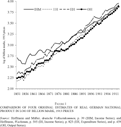
The net national product at factor costs or market prices can be calculated in three ways: from the expenditure, income, and output sides. In the national accounting scheme, the three approaches are based on the expenditure, output, and income accounts and should lead to identical aggregates. In Germany, national accounting started in 1891, and up to World War I only the income series were calculated by the Kaiserliche Statistische Amt (Imperial statistical office). The German economist, Hoffmann, estimated in two seminal contributions national accounting figures for Germany (see Figure 1).5
Hoffmann, Wachstum; and Hoffmann and Müller, Volkseinkommen.
As can be seen, the four series differ significantly, because of estimation errors and because they represent different national product concepts.
FIGURE 1 COMPARISON OF FOUR ORIGINAL ESTIMATES OF REAL GERMAN NATIONAL PRODUCT IN LOG OF BILLION MARK, 1913 PRICES
Some time ago Fremdling pointed out that there are large differences in the levels of these series, and recalculations for the early 1850s indicate that Hoffmann understated the true level of economic activity in Germany.6
Fremdling, National Accounts (1988). and National accounts (1995); and Hoffmann, Wachstum. Differences between the income, output, and expenditure series are well known for other countries, e.g., for the United Kingdom, see Nicholas Crafts, Recent Research; and Greasley and Oxley, Balanced versus Compromised Estimates.
So far, however, German national accounting figures for the nineteenth century have not been re-estimated.
7 Ritschl and Spoerer, Bruttosozialprodukt, present a re-estimation for the years 1900 to 1995.
The recent literature presents two approaches to the re-estimation of historical national accounts. First, the “structure-approach” of Christina Romer applies statistical relationships between national accounting sub-series from modern times to historical data.8
Romer, Prewar Business Cycle. Another approach in this line of research is Solomou and Weale, Balanced Estimates.
Second, the “new-data-approach” of Nathan Balke and Robert Gordon uses additional historical data to improve former estimates.
9 Balke and Gordon, Estimation.
The second approach uses more information, and it is therefore more efficient than the first. We decided to follow mainly the “new-data-approach.” In the following we discuss the expenditure, the output, and the two income approach series. Furthermore, we assess the quality of the four estimates and present our improved estimates.
The central piece of Hoffmann's book is the output-series, which we label OH. It is based on a voluminous investigation of production figures for many sectors.10
Hoffmann, Wachstum, p. 344, discusses the quality of his data. The data quality seems to be good after about 1870.
In general, output series are calculated from the production side by adding up the net value added of the different sectors. However, value added data were not collected by the statistical offices. Hoffmann bases his estimates on output quantities, not values, and employment figures. The calculated production index is linked to a base measure of output in 1913.
One major problem is the calculation of the industrial production index by Hoffmann, which was criticized by Fremdling, and especially Holtfrerich.11
Hoffmann, Wachstum, p. 390; Holtfrerich, Growth; and Fremdling, National Accounts (1988) and National Accounts (1995). For the interwar years, Ritschl, Spourious Growth, critizised the calculation of output in the metal processing industry, which is based on labor income and the assumption of a constant labor income share, not on production figures. This means that a large part of the output series is constructed from income data.
Hoffmann transforms the production indices of 12 industries into a Germany-wide industrial production index by multiplying the 1936 net production value per employed with the number of employed in the 12 industries using employment figures from census data.
12 Hoffmann, Wachstum, p. 389.
He therefore assumes a constant relative industrial productivity for the subsectors during the years 1850 to 1959, the years covered by Hoffmann's study. The 1861 employment census is used for the years 1850 to 1872, the 1882 census for the years 1872 to 1895, and the 1907 census for the years 1895 to 1913. Finally, Hoffmann estimated the value of industrial production for 1913 by multiplying the total industrial employment with the average industrial wage, and by adding the product of the estimated industrial capital stock and return-on-capital.
13 Hoffmann, Wachstum, p. 459.
He then applies his industrial production index to the 1913-industrial production value to calculate the value of industrial production for the years 1850 to 1913 in 1913-prices.
14 Wagenführ, Entwicklungstendenzen, p. 47, calculated an industrial production index for Germany starting in 1860 by combining physical output series of 57 industries. His weighting scheme is based on 1907 employment and the amount of horsepower installed. He conceeds on p. 13 that his constant 1907 weights lead to an underestimation of industrial production in the early decades, which is one of our major concerns regarding Hoffmann's index.
We improve this method by using additional industrial employment data given by Hoffmann.15
Hoffmann, Wachstum, p. 196.
Thus, data from the Zollverein-censuses of 1846 and 1861, and Prussian census data (for 1846, 1849, 1852, 1855, 1858, 1861, and 1867) are used.
16 Germany-wide data on employment are only available from Zollverein's censuses in 1846 and 1861. This information is included. Furthermore, Prussia covered around 60 percent of total employment, and comparison of the Prussian data with Zollverein data shows that the employment shares of different sectors were quite similar.
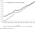
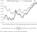
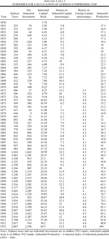
In addition, we linearly interpolated the data instead of using stepwise constant employment multipliers. Our re-estimated index of industrial production is compared with the original Hoffmann-index in
Figure 2, the data are in the
Appendix Table 3.
FIGURE 2 INDEX OF INDUSTRIAL PRODUCTION, 1851–1913. 1913 = 100, IN LOGS
The main difference between Hoffmann's index of industrial production and our newly calculated one is the higher level of industrial production in 1851. The annual growth rates are around 2.9 percent for the new index, and 3.9 percent for Hoffmann's index. The difference in levels can be explained by the different employment multiplier scheme. For 1851 we take linearly interpolated employment weights between 1849 and 1852. Hoffmann, on the other hand, used 1861 employment shares, thereby giving a higher weight to those subsectors with higher employment growth in the period 1851–1861. Thus the level of physical production is weighted too strongly for the fast-growing sectors. Thus Hoffmann's production index should be smaller than our index, which is calculated with more accurate weights.17
A similar argument holds for the jump in Hoffmann's industrial output index in 1872. Assuming that some industries grew faster than others over the entire period 1861–1882, then these sectors will be underweighted in 1871, and overweighted in 1872 after the change to the weights of 1882.
This higher level of economic activity for the early years conforms well to the views expressed by Holtfrerich and Fremdling.
18 Holtfrerich, Growth; and Fremdlig, National Accounts (1988) and National Accounts (1995).
Especially Holtfrerich finds higher values of industrial production.
19 The income per industrial worker in the Hoffmann data appears to be implausibly low. It is well below the NNP per employed, namely 555 M vs. 707 M in 1851. Our data, on the other hand, give a labor productivity of 1,165 M for the industrial sector, whereas the entire economy has a productivity of 862 M. Only as late as 1908 Hoffmann's industrial workers produced more than the average employed in the economy.
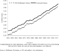
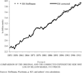
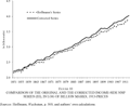
Because this article presents not only a new index of industrial production, but also new figures for the capital stock and the return-on-capital, the value of 1913-industrial-production also changes, because it is calculated by multiplying the number of employed with the average wage and adding the capital stock multiplied by return on invested capital. Furthermore, output series in general give Net Domestic Product at factor costs. We adjusted the series by adding indirect taxes to get NDP at market prices and then foreign income to get NNP. The change from NDP to NNP is less than 1 percent. The change from factor cost to market prices is about 5 percent, which explains the main component of the level difference. Figure 3 presents Hoffmann's estimate and our new estimate of German NNP calculated from the output side. The corrected series exhibits higher values than the old estimate and the difference between the two series increases over the course of the period. The level increase is mainly due to adding a new estimate of indirect taxes, because the output series represents NNP at factor costs. We present all series at market prices for reasons of comparability.
FIGURE 3 COMPARISON OF THE ORIGINAL AND THE CORRECTED NNP CALCULATED FROM THE OUTPUT SIDE, IN LOG OF BILLION MARKS, 1913 PRICES.
For the calculation of an NNP estimate from the expenditure side, Hoffmann estimates private and public consumption, net investment, and exports and imports; we label this series EH.20
Hoffmann, Wachstum, p. 825. In fact, Hoffmann (Wachstum, p. 667) estimated private consumption by subtracting exports minus imports, net investment and public consumption from production because there is little direct information about private consumption. Public consumption was estimated by using government budgets. Therefore, estimation errors in the output series are transmitted to the expenditure series.
One of the main problems is the calculation of investment expenditure for the secondary sector. In fact, Hoffmann estimates a capital stock index for Germany based on capital tax (Gewerbekapitalsteuer) data in the Grand Duchy of Baden, a small state in southwestern Germany. From these tax records Hoffmann estimates the capital stock in Baden. He then extrapolates it to Germany by multiplying it by around 31, a number supposed to reflect Baden's share of total industrial employment and its overall economic size. He derived the annual capital stock by multiplying the thus calculated index value by a capital stock estimation for 1913. This base year estimation is independent from the Baden figures, because it is based on additional data for the years 1925–1929.
21 Hoffmann, Wachstum, p. 240.
The yearly change of the thus-calculated capital stock is the net investment Hoffmann used in his expenditure series. Therefore, the expenditure approach excluded depreciation and leads to an NNP at market prices, not to a GNP. Schremmer, based on the same and additional archival records, recalculates Hoffmann's base figures for Baden.
22 Schremmer, Die badische Gewerbesteuer.
Schremmer accounts for changing tax legislation in this state, a fact left out by Hoffmann.
23 Schremmer, Die badische Gewerbesteuer, focuses on data quality and says little about the extrapolation of Baden data to Germany.
He ends up with investment figures, which are significantly higher than Hoffmann's figures for the years up to 1877. In other words, Hoffmann's NNP at market prices is too low.
In addition, Hoffmann assumes that Baden's industrial structure is representative for Germany as a whole. This is unlikely, as the “first industrialization” from the 1840s to the 1860s was concentrated in the Ruhr-basin and in Silesia, two areas with a significant share of heavy industry. Thus, Hoffmann's assumption of an equal capital intensity of the industrial sector in Baden and in Germany is problematic. This assumption would make sense if the industrial employment structure in Baden mirrored the German structure and if employment development in Baden and in Germany were equal. The use of employment census data does not confirm these assumptions.24
Employment data for Germany are given in Hoffmann, Wachstum, p. 182. Comparable data for Baden are available in Köllmann, ed., Quellen, pp. 23–26, and pp. 58–87 for 1846, 1861, and 1875. For 1882 and 1895 see Kaiserliches Statistisches Amt, ed., Statistik (1899), p. 252; for 1907 see: Kaiserliches Statistisches Amt, ed., Statistik (1910), p. 254.
Baden's share of industrial employment in Germany declined from 3.7 percent (1846) to 3.3 percent (1895); it then rose to 4.0 percent (1907). Even more problematic is the structural change within the industrial sector. For example, in 1846 the employment share of metal production and the metal working industry (Metallerzeugung- und -verarbeitung) was 19 percent in Baden, but only 10 percent in Germany. In Baden, this share remained constant until 1882, whereas in Germany it rose to 15 percent. Thereafter, the employment share in Baden rose to 24 percent (1907), and in Germany to 21 percent. Thus, the employment share of the capital-intensive metal industries doubled in Germany during these decades, but rose only about 20 percent in Baden. On the other hand, textiles had an employment share of 29 percent in 1846-Baden, but 48 percent in Germany. This changed by 1907: then, 20 percent were employed in textiles in Baden, but 27 percent were in textiles in Germany. Thus, the growth of capital-intensive industrial employment was much stronger in Germany than in Baden, and Hoffmann does not take account of this fact. To quantify capital intensity, information about subsectoral capital intensities is necessary.
Unfortunately, we do not have data on the capital intensities of industrial subsectors in nineteenth-century Germany. Thus, we decided to use information from modern Germany. We assumed that the average relative capital intensity during 1970 to 1994 equals the relative capital intensity during the nineteenth century, using the capital intensity in construction as numéraire. For example, we assume for the chemical industry a capital intensity of 5.9 times the capital intensity of construction.25
The multipliers for the others subsectors are: 5.1 (building materials), 5.5 (metal production), 2.2 (metal works), 3.6 (textiles), 3.5 (leather and paper), 1.1 (clothing), 2.1 (wood), and 3.8 (food). The relevant data on employment and capital stock were made available from the Statistische Bundesamt and are available on request.
Taking capital intensities from the late twentieth century might not accurately reflect the economic structure of the period under consideration. We checked the multipliers by deriving proxies of capital intensities from a study by Ernst Engel, who reported the horse power of steam engines in different industries for the year 1878.
26 Engel, Das Zeitalter des Dampfes.
Furthermore, he estimated the capital cost of steam engines per horsepower and the capital cost of connected machines. Thereby we were able to calculate capital intensities. The Pearson rank correlation with the modern data is 0.89.
27 We compared our estimates with estimates taking British capital intensities for 1920 (data are from tables 101 and 130 of Feinstein, Statistical Tables). The Pearson rank correlation between German capital intensities of 1970–1994 and British intensities of 1920 is 0.65. As another robustness check, we used data from the 1936 industrial census (Reichsamt für Wehrwirtschaftliche Planung, Deutsche Industrie- und Gesamtergebnisse, pp. 25–29, 44–55). We took the published ratio of capital income to total income per subsector as a proxy for capital intensity of the subsectors. These intensities give a Pearson rank correlation with the modern German data of 0.55. Fremdling and Stäglin (Industrieerhebung, p. 422) point out that these census data are distorted because of military-strategic consideration, which explains why we did not employ these data.
We are thus confident that the use of modern capital intensities will not seriously bias our results.
We compute an index value of capital intensity of subsector i as the ratio of capital per worker in the subsector i relative to the construction subsector's capital per worker
. This relative capital intensity Ki is multiplied by the employment share of the subsector i in Baden respective to Germany. This yields the index value of capital intensity of the entire industrial sector in Germany and in Baden.
28 The exact figures are for Baden / Germany: 3.03 / 2.55 (1846), 3.08 / 2.60 (1861), 2.87 / 2.68 (1875), 3.17 / 2.68 (1882), 3.20 / 2.68 (1895), and 3.05 / 2.70 (1907). For the years between the census years we linearly interpolated the coefficients. In Baden, the average relative capital intensity was constant or declining during 1846 to 1875, whereas in Germany it rose during these decades. Thereafter, the average capital intensity remained constant in Germany, but rose in Baden.
The ratio of the two is the employment structure factor
S. S is multiplied by the employment share factor and the absolute capital stock of Baden to derive the total capital stock for the Reich. More formally, the employment share factor is calculated as
E = LReich /
LBaden, the employment structure factor as
where K is the capital stock, L is the number of employed, the index i represents the industrial subsectors. The capital stock is thus KReich = KBaden * E * S. The thus-calculated capital stock is transformed into an index with the base year value 100 for 1913.
29 The base year capital stock estimation was originally calculated by Ferdinand Grüning, Versuch, pp. 14–18, and subsequently used by Gerhard Gehrig, Zeitreihe, pp. 13–15. Because Schremmer presented data only up to 1912, we assumed Hoffmann's 1913/12 annual capital stock growth rate to be correct. In addition, by multiplying the Baden capital stock with the employment share and employment structure factor, we end up with a capital stock estimation (in 1913 prices) about 35 percent lower than Hoffmann's estimation for 1913. Such a difference is possible because Schremmer, Die Badische Gewerbesteuer extensively describes the systematic undervaluation of the Baden capital stock. This undervaluation was part of industrial policy, because it lowered the tax base for companies in Baden and thus fostered industrial development in the Grand Duchy of Baden.
Because we add information about total industrial employment and industrial employment structure, we do not use a constant multiplier (
E *
S) as Hoffmann did.
So far, Hoffmann's and our capital stock estimate depend on the Baden capital tax. However, we can complement the index by a second capital stock index calculated from company balance sheet data for 44 large joint-stock companies for 1885–1913 based on a sample by Rudi Rettig.30
Rettig, Investitions- und Finanzierungsverhalten.
This sample covers the main industries and the main industrial regions. Rettig's data do not include any firms from Baden. The two samples are thus independent and we calculate a second index based on Rettig. We thus employ for 1850–1884 the improved Baden series, thereafter an average of the improved Baden series and the independently calculated Rettig index. The weights given to the samples are one-third for Baden and two-thirds for Rettig respectively and are based on average capital stock during 1885–1912.
31 Rettig's and Baden's data jointly cover nearly 10 percent of the German industrial capital stock, thus our sample is significantly larger than Hoffmann's for the 1885–1913 period.
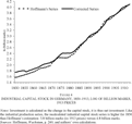
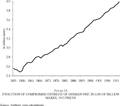
Finally, we multiplied our index value with Hoffmann's 1913 capital stock estimation. Figures 4 and 5 show our corrected capital stock and net investment series; the data are in Appendix Table 3.
FIGURE 4 INDUSTRIAL CAPITAL STOCK IN GERMANY, 1850–1913, LOG OF BILLION MARKS, 1913 PRICES
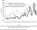
FIGURE 5 MANUFACTURING AND NONMANUFACTURING INVESTMENT: HOFFMANN'S AND NEW ESTIMATE, MILLION MARKS, 1913 PRICES
The investment data are presented in Figure 5.32
Gehrig, Zeitreihe, connected Grüning's (Versuch) estimate for the capital stock in 1913 with Wagenführ's (Zur Entwicklung) volume index of investment. The result is a gross investment series for the total economy, a series not comparable to net investment series. Grabas, Konjunktur, p. 452, presents an investment series only from 1906–1913, based on IPOs and capital increases of joint stock companies. We do not further consider this series for two reasons: The series is short and the link between capital issues and investment in the entire economy is not self-evident.
A comparison of the original Hoffmann and our industrial investment reveals some difference in cyclical behavior. A shift in investment behavior can be noticed during the 1870s and late 1880s. Although Hoffmann had an investment peak in 1871, the improved data only exhibit a peak in 1873, but with a high level of investment until 1876. Similarly, in the 1880s Hoffmann's data show a sustained high investment from 1886–1890, whereas our data have two small downturns in this period. Finally, after about 1900 Hoffmann's peaks lead ours by one to two years.
As a robustness check we compare the two industrial investment estimates with nonindustrial investment. Hoffmann also presents independently estimated figures for non-industrial-sector investment.33
Hoffmann, Wachstum, p. 827.
According to his estimation, nonindustrial net investment starts to grow in 1872, a process lasting until 1876, and followed by a decline until 1880. This record of the non-industrial sector investment roughly mirrors the development of our new series. Turning to the early twentieth century,
Figure 5 shows a shift of peaks and troughs. However, the revised Baden data and Rettig's data, which were employed to construct our industrial investment index, closely co-move and both show the same cyclical pattern.
34 After 1885 our cyclical pattern is based on two independent data series, the Baden-tax-series and Rettig's data.
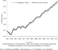
We include the new industrial net investment series into our revised EH expenditure series (
Figure 6).
FIGURE 6 COMPARISON OF THE ORIGINAL AND THE CORRECTED EXPENDITURE SIDE NNP, LOG OF BILLION MARKS, 1913 PRICES
A further important topic related to the EH series is the calculation of the implicit deflator. Hoffmann presents the expenditure series in nominal terms as an NNP and in real terms as an NDP (Net Domestic Product).35
Hoffmann, Wachstum, p. 825.
From the nominal series we subtracted the nominal current account balance to get the nominal NDP. The ratio of nominal to the real NDP then gives the implicit NDP deflator. We compared this deflator with the consumer price index (CPI) of the Imperial Statistical Office, which is available for the period 1881–1913 and with two wholesale price indices presented by Alfred Jacobs and Hans Richter.
36 Hohls, Sectoral Structure; and Jacobs and Richter, Groβhandelspreise.
The official CPI exhibits little difference to the implicit NDP deflator for the available period, whereas Jacobs and Richter depicts a differing cyclical behavior.
37 Jacobs and Richter, Groβhandelspreise.
Thus in this period the implicit NDP deflator appears to be superior to Jacobs and Richter's estimate. In addition, Jacobs-Richter is a wholesale price index for industrial and agricultural goods only, whereas the implicit deflator derived from Hoffmann's data is an NDP deflator. In earlier years (before 1878), the Jacobs-Richter index has a significantly higher level than Hoffmann's data and converges to Hoffmann's level during 1874–1878. This difference can be explained: As pointed out, the Jacobs-Richter index is a wholesale price index of agricultural and industrial goods. In the 1870s, however, the relative prices of industrial goods compared to nonindustrial goods decreased. Therefore the Jacobs-Richter index overestimates the general price level in the period preceding the 1880s because industrial goods were relatively more expensive. We decided to deflate our series and most of our sub-series with the implicit NDP deflator used by Hoffmann.
38 Only the capital stock subseries is deflated by a different price index.
The third national accounting approach uses factor income. National income is calculated by adding up labor and capital income in the economy.39
Rent income and profits are included in capital income.
There are two independent estimates available, one by Hoffmann, and a second by Hoffmann and Müller. Both series lead to an NNP at factor costs in current prices.
40 Hoffmann, Wachstum, p. 505; and Hoffmann and Müller, Volkseinkommen, p. 39.
Hoffmann estimated the national income by using employment census data, multiplied with the average annual income of employees in the respective subsectors of the economy.41
Hoffmann, Wachstum, p. 505.
This product gives the labor income of the economy. Capital income is calculated by applying a constant rate of return on the economy-wide capital stock. As already discussed, Hoffmann's capital stock estimation for the industrial sector is too low. In addition, he assumes a constant profit rate on this capital stock of 6.68 percent, a rather low value as Fremdling points out.
42 Fremdling, National Accounts (1995), p. 88. The rate of return for the other nonagricultural sector is constant at 4.788 percent.
We use here our corrected capital stock series and apply a newly estimated rate-of-return to this capital stock.
Because comprehensive data on company profitability are not available, we decided to use dividend yields of joint-stock companies as a proxy. Dividends should be high in times of high company profitability and low in times of bad performance and are probably a good proxy. However, for the early years it might be problematic, because the German joint-stock companies law was liberalized in 1870, and before that date, the number of joint-stock companies was rather low. Further, joint-stock companies are mainly large corporations. Small and medium size companies are thus not covered by the sample. Two types of information are needed for our calculation: first, a time series on the average dividend yield at the German stock market; second, data on the relation-ship of company profits to dividends. Time series evidence for the dividend yields is available for the years 1870 to 1913.43
Donner, Kursbildung, p. 98.
For the period 1851 to 1869 we estimated the dividend yield from a sample of 11 joint-stock companies in 1851; 31 in 1856, 99 in 1862; by 1869 our sample covers 166 companies.
44 Van der Borght, Statistische Studien, p. 222.
Our data are thus quite reliable for the 1860s. The profit-dividend relation is calculated using a cross-section of 375 joint-stock companies for the year 1880.
45 Van der Borght, Statistische Studien, p. 290.
We assume the profit-dividend ratio to be constant at 1.189 for the years 1851 to 1913.
46 We checked the assumption of a constant profit-dividend relation with data from 50 industrial firms and nine banks covering the years 1880–1913 taken from Rettig, Investitions- und Finanzierungsverhalten; and Burhop, Executive Remuneration. In this period the ratio was nearly constant.
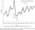
We estimate the average return on capital to be 9.63 percent during the years 1851–1913, but the new series, which can be seen in
Figure 7, fluctuated around this mean.
47 There could be a bias in this estimate if the “surviving” companies receive a larger return on capital than a sample of all companies. Tilly, Public Policy, calculated an approximate survivor bias of joint stock companies. He showed that during 1871–1883 the stock market return of 489 companies was 2.6 percent, whereas the stock market return of the 294 surviving companies was 4.4 percent. Adjusting our return by this percentage difference, however, has very little influence on national income. Tilly's data are furthermore not really comparable to our return data, because we have return on capital, whereas Tilly calculates stock market return. In addition, the period 1871–1883 was marked by significant stock market fluctuations. Furthermore it can be assumed that the survivor bias is procyclical, thereby our data should underestimate the cycle.
FIGURE 7 RETURN ON INDUSTRIAL CAPITAL IN PERCENTAGES, 1851–1913
We checked the quality of our profit-rate estimation with the independent data set by Eduard Wagon.48
Wagon, Finanzielle Entwicklung, pp. 175–212. This data set informs us about capital and profits of a large sample of joint-stock companies for the years 1870 to 1900. The sample covers 93 companies in 1870, 430 in 1880, and finally 830 in 1900. The two estimations are quite similar, with a correlation of 0.8. The only major difference occurs during the stock-market boom of 1872/73, but even this difference of around 11 percent leads to an NNP estimation error of less than 1.5 percent. We therefore think that our profitability estimation is quite reliable.
also presents this alternative, estimated rate of return. Wagon's and our estimate based on the data by Richard van der Borght and Otto Donner have similar properties, we therefore believe that our estimate accurately depicts the return on capital in the investigated period.
Because we calculate NNP and not NDP, the income series IH includes foreign income.49
Hoffmann, Wachstum, pp. 261 and 510.
Foreign income consists of capital and labor income. Hoffmann assumes that there was no net foreign labor income. He thus looked only at capital income. In addition, he assumed a net total investment of 20 billion marks for 1913, and he assumed zero investment for 1871 and the years before. We do not change Hoffmann's foreign asset series, but do change his rate of return. He assumed a 3 percent rate of return for 1913, and he calculated this rate backward by using a seven-year moving average of German long-term bonds. Instead, we are using the rate described above (
Figure 7) of return for the German inland capital stock and data on the return at the German bond market.
50 Donner, Kursbildung, p. 98.
The portfolio-mix (bonds vs. shares) is given by Hoffmann.
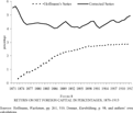
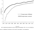
Figures 8 and
9 present the applied rate of return and the net foreign income.
FIGURE 8 RETURN ON NET FOREIGN CAPITAL IN PERCENTAGES, 1870–1913
FIGURE 9 NET FOREIGN INCOME, IN LOG OF MILLION MARKS, 1870–1913 (1913 PRICES)
Figures 8 and 9 show an upward correction of the international rate of return and therefore also of Hoffmann's total foreign income data. His rate of return in the earlier decades appears to be implausibly low. In addition, because our interest rate is not smoothed, the cyclical behavior of international income is better captured by our series. Our interest rate estimation represents a lower bound, because we assume the same interest rate for national and foreign investments. Thus, no risk premium is contained in our series. Karl Christian Schaefer shows a higher return for international investments than for national investment for some countries.51
Schaefer, Deutsche Portfolioinvestitionen.
However, representative figures on investment abroad are not available. See
Figure 10 for our correction to the IH series.
FIGURE 10 COMPARISON OF THE ORIGINAL AND THE CORRECTED INCOME-SIDE NNP SERIES (IH), IN LOG OF BILLION MARKS, 1913-PRICES
Hoffmann and Müller present a second income estimate, NNP at factor costs, based on the official income calculation of the Kaiserliche Statistische Amt, which published such a series from 1891 onward, See Figure 11.52
Hoffmann and Müller, Volkseinkommen, p. 39.
Hoffmann and Müller extend the official series back to 1851 by using archival material from several tax offices, starting with Prussia in 1851.
53 We linearly interpolated this income series for the missing values in 1867, 1868, and 1870.
Data for other states become available from 1871, and for 1913 over 90 percent of population is covered by these data.
54 From 1851 to the mid 1860s, Prussian data cover around 48 percent of the German population. After the “unification wars” (1864–1866), this figure rose to 60 percent. Prussia was a very heterogeneous state (agriculture in the east, industry in the west) and later studies showed that the Prussian income development was representative for Germany. For 1874, data from Prussia, Saxony, Hesse, Hamburg, and Bremen are available and 70 percent of the German population is covered.
We label this series “IHM.”
FIGURE 11 COMPARISON OF THE ORIGINAL AND THE CORRECTED INCOME-SIDE NNP ESTIMATE (IHM), IN LOG OF BILLION MARKS, 1913 PRICES
Four shortcomings of tax office data are raised by Ritschl and Spoerer.55
Ritschl and Spoerer, Bruttosozialprodukt, p. 30.
The taxation base is only large enough to compute precise estimates after the Prussian tax reform of the early 1890s and similar reforms in other states. A second problem is the fact that tax payers declared only a part of their income.
56 Hoffmann and Müller, Volkseinkommen. After the introduction of the new Prussian income taxation code in 1891 this problem became apparent. Hettlage, Finanzverwaltung, briefly describes the German taxation system. The highest tax rate on income in Prussia was 3 percent, incentives to evade taxes were thus rather low. Yet, one should note that the state income tax was supplemented by local income taxes and thus the tax rate could be as high as about 9–10 percent in some Prussian cities.
Hoffmann and Müller corrected for this bias using results of a 1913 Reichstag commission.
57 This bias appears to create a level rather than a cyclical difference.
Third, there was a tax-free minimum income, which is not covered in the data. Hoffmann and Müller address this issue by taking an estimate of the average income below the tax-threshold in 1913. They extrapolated this number backwards using a wage index. The total tax free income was then calculated by multiplying the number of employed people less the number of tax payers with the average below threshold income.
58 The income distribution is stable over time. In Saxony—other data are not available—the lowest quartile of the population earned 8.2 per cent of the total income in 1874, and 7.2 percent in 1913 as calculated from Jeck, Wachstum. The bias from this source seems quite small.
Fourth, before the reform of 1891, two types of income were distinguished in Prussia: fixed (“fundiert”) and variable (“unfundiert”) income. Fixed incomes were taxable in the year of payment, whereas in the case of variable incomes, taxes had to be paid one year after the income flow. Sometimes these incomes were averaged over the last three years. This means for business cycle analysis that the cycle could be shifted and dampened. Because large parts of the population are covered by the taxation base approach, the data are relatively reliable even before the 1890s.
Both income series, IH and IHM; and the output series OH yield an NNP at factor costs, not an NNP at market prices like EH. We thus add taxes on production and imports (indirect taxes) to get NNP at market prices.59
We left out any corrections for subsidies because in 1913 they amounted to only 30 million marks, whereas the indirect taxes were around 2,867 million marks.
Spoerer calculated the indirect taxes for 1901 to 1913, and he roughly guessed that the growth rates of indirect taxes for Germany was around 7 percent from 1850 to 1880, and circa 1 percent from 1880 to 1900.
60 We used a mean value of 4 percent. Starting with Spoerer's figure for 1901, we calculated the amount of indirect taxes backward to 1851 by using this growth rate guess.
61 We deflated the indirect taxes with the Hoffmann implicit NDP deflator discussed above. There is no generally accepted way of deflating tax revenues, however, these taxes are levied on a wide range of products and thus using an NDP deflator seems appropriate.
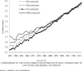
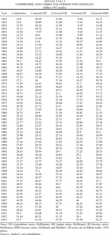
The resulting four estimates of German NNP at market prices are presented in Figure 12. The data are in Appendix Table 2. To summarize our main corrections: We add new net investment data to the expenditure series (EH), new industrial production figures and foreign income to the output series (OH), capital income and foreign income corrections to the income series (IH). In addition, indirect taxes were added to OH, IH, and IHM. Therefore, we have four NNP series at market prices. National accounting requires them to be equal, differences in the series are thus a result of imprecise estimations. There are important level differences in the new series. Especially in the 1850s and 1860s the IHM series is considerably higher, also it has more pronounced cyclical movements. In 1892 the four series almost converge and the differences between the series stay relatively small.
FIGURE 12 COMPARISON OF THE FOUR CORRECTED ESTIMATES OF REAL GERMAN NNP, IN LOG OF BILLION MARKS, 1913 PRICES
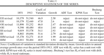
Table 1 presents summary statistics of the four revised and of the four original series. The coefficient of variation of the four series varies. The IHM series has the lowest coefficient of variation and also the lowest standard deviation, it is thus the smoothest series with the fewest fluctuations. The IH series on the other hand has the largest coefficient of variation. The EH and OH series are in between, they also differ somewhat.
Since the work of Charles R. Nelson and Charles I. Plosser it has become standard to test macroeconomic time series for the existence of stochastic trends (unit roots).62
Nelson and Plosser, Random Walks.
This has fundamental implications for the analysis of business cycles, because in the case of a unit root all innovations to the series have permanent effects, while in the case of a deterministic trend, innovations will only have temporary effects. We employed the augmented ADF test, which has the null hypothesis (
H0) of unit root. We were able to reject
H0 for the series EH and for the revised IH. However, the ADF test has low power to reject compared to near unit root alternatives.
63 See, for example, Rudebusch, Uncertain Unit Root.
We therefore also employed the KPSS test, which tests the
H0 for trend stationarity.
64 The optimal truncation lag length was calculated according to an automatic bandwidth selection routine as presented in Hobijn et al., Generalizations. The routine is implemented in STATA. The optimal truncation lag was five for all series.
In all cases we were able to reject trend stationarity except for the EH series. As a further unit root test, we employed the test developed by Jörg Breitung.
65 Breitung, Nonparametric Tests
Breitung's variance ratio statistics is similar to the test statistics suggested by KPSS, but it assumes nonstationarity under the null hypothesis. The results of the Breitung test are in line with the results of the KPSS test. We therefore conclude that the IHM, IH, and OH series, both the original, as well as the revised, exhibit a unit root. The EH series, on the other hand, is trend stationary.
66 The unit root tests were conducted on the log-transformed series. We performed the unit root tests in addition on the original series. In this case, all four series have a unit root.
FLUCTUATIONS AND LONG-TERM TRENDS IN GERMAN NNP
Long-Term Trends, 1851–1913
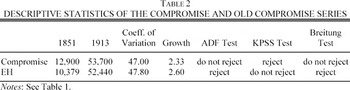
The average yearly growth rate of the compromise is 2.3 percent. As mentioned previously, this growth rate is lower than that of the often employed EH series. The growth rate difference of 0.3 percent annually reduces the 20-percent initial level difference to nearly zero.
A graphical analysis of the log-transformed compromise does not reveal a break in the trend growth rate. A growth accounting exercise can be performed on this long-term growth rate and might yield additional insights because the new series not only exhibits lower growth rates, but also includes a higher capital stock series.74
Note that our economy-wide capital stock series includes the value of land. Hoffmann did not include it in his economy-wide capital stock. On page 234, Hoffmann presents the value of land in current prices and on page 569 the land price index. Dividing the two indices gives a constant value of land in 1913 prices of 73 billion. This implies that TFP growth is high, because a large part of the capital stock is fixed.
Starting from a linear homogenous production function (for example, a Cobb-Douglas type) and factor remuneration at marginal product, growth of output can be decomposed into the contribution of growth of capital, labor, and a remaining term, the Solow residual, which is interpreted as a measure of the contribution of technological progress. Employment and capital growth must be weighted by the respective income shares of the factor. We took the average income share of capital for the entire period, which is 0.244 for the Hoffmann's data and 0.241 for the revised data.
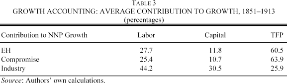
Table 3 shows that the relative importance of the three factors labor, capital, and technology is altered by our data modifications: Labor and capital accumulation contribute less to growth than before; total factor productivity (TFP) gains importance. Because TFP is calculated as a residual, a smaller part of growth can be explained with the new data.75
Schremmer (Wie gross war der ‘technische Fortschritt’) did a similar exercise with Hoffmann's original IH series. He calculated a TFP share of 43 percent, a value close to our calculation with the EH series if we do not include land. Schremmer neglected the role of land as capital in production.
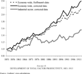
Figure 15 shows the evolution of TFP over time, normalized to 1851 equals one. Both decompositions for the NNP give a tremendous increase in TFP of 158 percent with the old data and 182 percent with the revised data. The TFP level of the revised data is similar or larger than for the unrevised data for the entire period.
FIGURE 15 DEVELOPMENT OF TOTAL FACTOR PRODUCTIVITY, 1851–1913
This residual TFP growth is unexplained by growth accounting. According to Broadberry, structural change within the German economy could be a reason for increased TFP growth.76
Broadberry, Productivity Race.
Factors were reallocated from low-productivity agriculture to high-productivity manufacturing, which increased the aggregate productivity level of the economy. In fact,
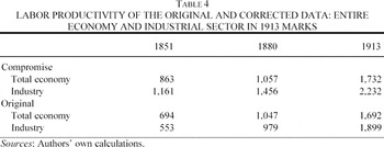
Figure 15 shows that TFP growth in the industry sector was much lower than for the entire economy, growing only by 57 percent. Performing standard growth decomposition for the industry sector it can be seen that growth of this sector was mainly driven by additional labor input. One reason for this additional labor input is the labor productivity difference between industry and the other sectors as can be seen in
Table 4. Over the entire period the labor productivity was always higher in the industrial sector for the corrected series. Workers therefore had an incentive to move to the industrial sector.
77 In the original series, until 1907 labor productivity was lower in the industrial sector, an unlikely finding.
Because we have production indices for each industry and employment data for each industry, we can decompose the growth of output into two components: A productivity component and the increase in employment. We calculated the average increase in the production index for each industry as the geometric mean of the yearly growth rates for the available years. Similarly, we computed the average growth rates of employment in each industry. Subtracting employment growth from production growth yields average increases in labor productivity for each industry for the investigated period. These labor productivity increases reflect two components that we cannot further decompose: increases in the capital stock per worker and increases in efficiency of the work process.
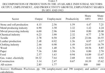
The average industrial output growth rate in the investigated period is 2.85 percent per annum (see Table 5).
Output, employment, and productivity grew in all industries. Employment growth in the investigated period was 1.77 percent per year. Output and also employment growth was highest in the gas, water, electricity, paper production, metal production, and the chemical industry. Productivity increases were similarly very high in these sectors. For 1851 the employment shares were highest in clothing, textile, food and wood production. The shares of textile and clothing, however, dropped significantly over the period by 10 percentage points. On the other hand, the metal processing industry and construction industry had significantly higher employment shares in 1913 than in 1851.
In a second step we can derive aggregate labor productivity increases by weighting the sectors with their 1851 employment share respective to their 1913 employment share. Aggregate annual productivity growth was 1.725 percent given the employment shares of 1851, and 1.848 percent given the structure of 1913. Thus, the structure of the economy changed such that sectors with a higher productivity growth increased their employment share.
The German Business Cycle, 1854–1910
In this section, we present and discuss the business cycle ramifications of the compromise estimate of German NNP for the years 1854 to 1910.78
Due to the filtering technique, we are losing the first and final three years
To obtain a business cycle, we need to decompose the univariate time series of German NNP into the components of a cycle and a trend. Numerous statistical techniques have been proposed for that purpose. Fabio Canova examines the business cycle properties of time series using a variety of detrending methods.
79 He shows that different filters extract different information from the time series. Thus, business cycles vary considerably with the choice of different filters.
80 Burhop and Wolff, Datenwahl and National Accounting, compare the cyclical properties of four German NNP estimates during 1851–1913 with four different econometric techniques. The four estimates by Hoffman, Wachstum; and Hoffmann and Müller, Volkseinkommen, are shown to have differing cyclical properties, irrespective of the methodology chosen. Furthermore, Burhop and Wolff find that business cycles in some periods vary with different methodologies.
Marianne Baxter and Robert King develop a band-pass filter, which allows the isolation of business cycle fluctuations in macroeconomic time series.
81 Baxter and King, Measuring Business Cycles. Another standard method, the Hodrick-Prescott (HP) filter, has been shown to generate artificial cycles if the series contains a unit root (Cogley and Nason, Effects). We therefore do not employ the HP filter. The HP cycle, however, looks very similar to our presented results, if λ = 100 as a smoothing parameter is chosen. The precise dates are in some cases shifted by a year for booms and recessions. Thus employing another nonstructural filter gives very similar results. We opted against employing a structural filter, such as a Kalman filter (for an application to historical data see Crafts et al., Climacteric).
The approximate filter extracts a specified range of periodicities, and otherwise leaves the properties of this extracted component unaffected. The filter does not introduce phase-shifts, so the extracted time series will also be stationary if the original series is integrated of the order two or less.
82 It is therefore irrelevant, whether we employ the log-transformed series or the original series. The filtered business cycle was in both cases virtually equivalent.
Furthermore, the extracted business cycle is unrelated to the length of the sample period. The filter is basically a moving average with weights chosen in such a way as to approximate the ideal filter, which only allows specified periodicities to pass. In their choice of periodicities Baxter and King follow the classical definition of Arthur Burns and Wesley Mitchell, who specified that business cycles were cyclical components of no less than six quarters and less than 32 quarters (eight years).
83 Burns and Mitchell, Measuring Business Cycles.
This filter thus has well determined properties, is very suitable for a business cycle analysis, and is employed here to extract the cycle.
Our main points of interest are booms and recessions.84
We do not investigate in detail questions such as the length of the cycle. For evidence on this in a historical context, see A'Hearn and Woitek, More International Evidence.
We define a boom as a period of actual NNP higher than trend NNP until it reaches the local maximum, a recession is defined as a period of actual NNP lower than trend NNP until the local minimum. In this context, “local” refers to the interval between two crossings of the trend line.
85 Other definitions of booms and recessions can be used. However, we believe that a boom should not start before the cycle crosses the trend line, because the economy would still be under the trend level of NNP. In addition, declines in NNP do not constitute a recession if NNP is still above the trend level.
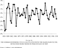
Figure 16 depicts the percentage deviation of actual NNP from trend NNP for the years 1854 to 1910 measured by the band-pass filter.
FIGURE 16 THE GERMAN BUSINESS CYCLE CALCULATED WITH THE BAND-PASS FILTER. DEVIATION FROM TREND IN PERCENTAGE OF NNP
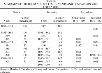
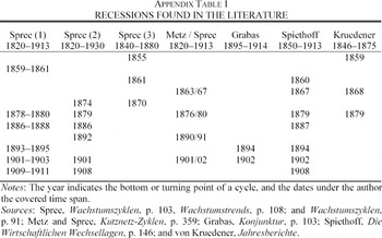
The business cycle reveals strong fluctuations during the late 1850s and early 1860s, thereafter the normalized cycle appears to be of constant magnitude. Table 6 shows the exact dates of booms and recessions, using our definitions and compares the dating with Knut Borchardt and Craig and Fisher who both employ the original EH series.86
Borchard, Wachstum und Wechsellagen; and Craig and Fisher, European Business Cycle, p 154. Appendix Table 1 summarizes the dating of recessions.
In total, 11 booms and 12 recessions are reported, with an average length of a cycle (from peak-to-peak) of around five years. Besides the dating we also report a measure of the intensity of a boom or a recession. For the intensity measure, we calculated the total trend deviation during a boom or recession period and divide this figure by the average total trend deviations of all boom respective recession periods.
The first decade under consideration can be characterized by very strong fluctuations: Two of the three strongest recessions and the strongest boom fall in the period 1855–1862. During the 1860s, many “noneconomic” factors influenced the German economic development, namely the “German unification wars” of 1864 and 1866, and in addition the American civil war. We find recessions in 1861–1862 and 1867, both deeper than average recessions. On the other hand, we report a very strong boom 1863–1864 and an upturn in 1869, which might have been put to an end by the German-French war. Indeed a small recession in 1870–1871 can be found. The typical “Gründerboom” from 1870–1873 can not be detected.87
The Gründerboom was the strong economic upturn after the foundation of the German Empire in 1871–1873. It was followed by a decline of economic activity in 1873–1879, the so-called Gründerkrise.
On the contrary, output was below trend in this period. Cyclical output resumed growth again in 1875, and in 1877 a small recession can be noted. Thereafter the economy boomed strongly in 1878 and 1879.
During the 1880s the German economy experienced a recession in 1880 and a minor downturn in 1886–1887. The prosperity phases of 1884 and 1888 were average expansions. The 1880 recession can be related to the new tariffs on imports, introduced in 1879, reducing imports significantly.88
Morgenstern, International Financial Transactions, p. 579.
For the 1890s we report a marked downturn in 1890–1892, and a minor recession 1895–1896, a prospering year 1893, and a true boom in 1898. This 1898 upswing was the strongest of the entire second half of the nineteenth century. The boom of the late 1890s, which Oskar Morgenstern relates to a strong and sustained rise in foreign trade, can also be related to a strong expansion of industrial production, a sustained increase in net foreign income, rising profitability of industrial investments, and an investment boom.
89 Morgenstern, International Financial Transactions, p. 579.
The twentieth century started with a deep recession 1900–1902 accompanied by a banking crisis. This recession was followed by two minor recessions in 1906–1907 and 1909–1910 and two prosperity phases in 1904–1905 and 1908.
The business cycle dating for the 1870s deserves a detailed discussion because it diverges from the commonly assumed pattern of “Gründerzeit”-boom (1870–1873) and “Gründerzeit”-crisis (1874–1879). This dating of boom and crisis rests on three data types: financial market data (stock-market, interest rate, foundation of new joint-stock companies, issues of stocks and bonds), monetary data (M2, inflation) and Hoffmann's data for consumption, investment, income, and production.
We first turn to the real side of the economy, namely industrial production (from the OH series), investment (from the EH series), and capital income (from the IH series). Hoffmann's and our indices of industrial production exhibit no substantial differences. The only exception is the year 1872, when German industrial production grew 17 percent according to Hoffmann, but only 7 percent according to our re-estimation. Our estimate is supported by Rolf Wagenführ's estimate as they are close.90
Wagenführ, Entwicklungstendenzen.
According to Hoffmann, the net investment in the industrial sector from 1870–1873 reached 2.74 billion marks (in 1913 prices); from 1874 to 1879 net-industrial-investment was 1.8 billion marks.
91 Our re-estimation leads to much lower investment figures for 1870–1873 (1.275 billion marks), for 1874–1879 it amounts to 1.448 billion marks. Thus, in the “boom” period our investment figures are less than half of Hoffmann's. Investment was very strong in 1872–1876, which could be related to the transformation of French reparation payments, which were finalized in May 1873, into real investment. One example for long-term real investment is railway construction (which is not included in industrial investment, but is closely connected with it via heavy industry). During the years 1871 to 1873, around 806 kilometers of new railway lines were constructed in Germany per year, but during 1874 to 1876, this figure rose to 1,805 kilometers. Furthermore, in line with our series, Hoffmann's data on nonindustrial investment show declining figures for 1871, and a strong investment record for the years 1874 to 1876.
92 Our claim of a good economic situation during the mid-1870s can also be supported by single-firm evidence. For example, the turnover of Krupp increased from 35 million marks in 1872 to 47 million marks in 1878, an increase of 34 percent, see Gall, Krupp, p. 202.
Our corrected capital income data show a peak in 1872, whereas Hoffmann has a peak in 1874–1875.
93 Thus the original IH peak is later than the EH and OH peak and not in line with the typical business cycle dating, see Burhop and Wolff, Datenwahl.
Because Hoffmann assumed a constant rate of return on capital, his capital income figures barely increase. Our rate-of-return series, on the other hand, shows a strong upturn which can be related to financial market developments.
Between August 1870 and November 1872, the stock market index doubled, mainly driven by positive expectations regarding the French reparation payments. This development is also reflected in our financial return series, which captures nonrealized profits on shares held by companies. This financial side of the economic development was the main source of information for the economic development used by contemporaneous authors, such as Max Wirth, Otto Glagau, and Herbert Blume, mainly because financial data were readily available, whereas national accounting data were not.94
Wirth, Geschichte; Glagau, Börsen- und Gründungsschwindel; and Blume, Gründerzeit.
In fact, the stock-market index peaked in November 1872 and collapsed during 1873. It reached the lower turning point during May 1877.95
Donner, Kursbildung, p. 98.
In the stock market boom, more than 900 new joint-stock companies with a total capital of nearly 2.8 billion marks (in current prices) were founded during 1871 to 1873. In terms of nominal share value, one-third of these companies were banks, that is companies without an immediate impact on the real economy. In addition, many of these banks were subject to stock-market speculation.
96 See Burhop, Kreditbanken, for an extensive discussion of joint-stock banking during the 1870s.
Looking at industrial companies, the foundation boom turns out to be much smaller: only 12 of the 100 largest German industrial companies (census year 1887) were founded during the early 1870s, but 31 of them were transformed into a joint-stock company. Thus, the industrial foundation boom was more a renaming boom, at least for the largest firms.
97 Data are from Kocka and Siegrist, eds., Recht und Entwicklung, pp. 55–122.
The boom recession pattern observed by the contemporaries was visible mainly in financial and monetary data, which do not necessarily reflect the real economic development.
An additional factor determining financial and monetary variables and the perception of real developments was the large gold inflow resulting from French reparation payments. It increased the money supply significantly, and no central monetary authority existed to sterilize the inflow of gold.98
The Reichsbank was founded in 1876 and its major policy goal was a stable exchange rate, not a low inflation rate.
M2 rose by 45.1 percent between 1870 and 1873, which in turn led to increasing prices.
99 Tilly, Zeitreihen, p. 347.
The average inflation rate from 1860 to 1869 was 0.55 percent, whereas the average inflation rate from 1869 to 1873 was 5.26 percent. If people inferred price expectations from past experience, they expected inflation to be far below the actual values. A further indicator of constant price expectations is the nearly unchanged nominal interest rate.
100 The nominal interest rate for Prussian government bonds was around 4.1 to 4.7 percent during the 1870s, Donner, Kursbildung, p. 98.
Companies, in view of rising prices for their own products and constant inflation expectations, increased production. Thus, they assumed a rising relative price of their products, whereas, in fact, the general price level rose. For the 1870s we can therefore conclude that financial and monetary data confirm the traditional account of the “Gründerzeit.” However, taking the currently available data on NNP as a basis for the business cycle dating, a divergent pattern emerges such that there was a small recession in 1870–71 and a small boom in 1875.