Nomenclature
-
 ${a_c}$
-
centripetal acceleration [ft/s2]
-
$b$
-
wing span [ft]
-
${C_D}$
-
drag coefficient [−]
-
${C_{{D_0}}}$
-
zero-lift drag coefficient [−]
-
${C_{{D_{da}}}}$
-
drag coefficient due to aileron deflection [deg−1]
-
${C_{{D_{de}}}}$
-
drag coefficient due to elevator deflection [deg−1]
-
${C_{{D_{df}}}}$
-
drag coefficient due to flap deflection [deg−1]
-
${C_{{D_{dr}}}}$
-
drag coefficient due to rudder deflection [deg−1]
-
${C_L}$
-
lift coefficient [−]
-
${C_{{L_0}}}$
-
zero-lift lift coefficient [−]
-
${C_{{L_{da}}}}$
-
lift coefficient due to aileron deflection [deg−1]
-
${C_{{L_{de}}}}$
-
lift coefficient due to elevator deflection [deg−1]
-
${C_{{L_{df}}}}$
-
lift coefficient due to flap deflection [deg−1]
-
${C_{{L_{dr}}}}$
-
lift coefficient due to rudder deflection [deg−1]
-
${C_{{L_q}}}$
-
lift coefficient due to pitch rate [rad−1]
-
${C_{{L_\alpha }}}$
-
lift coefficient curve slope [deg−1]
-
${C_{{L_{\dot \alpha }}}}$
-
lift coefficient due to alpha rate [rad−1]
-
${C_l}$
-
rolling moment coefficient [−]
-
${C_{{l_{da}}}}$
-
rolling moment coefficient due to aileron deflection [deg−1]
-
${C_{{l_{de}}}}$
-
rolling moment coefficient due to elevator deflection [deg−1]
-
${C_{{l_{df}}}}$
-
rolling moment coefficient due to flap deflection [deg−1]
-
${C_{{l_{dr}}}}$
-
rolling moment coefficient due to rudder deflection [deg−1]
-
${C_{{l_p}}}$
-
rolling moment coefficient due to roll rate [rad−1]
-
${C_{{l_r}}}$
-
rolling moment coefficient due to yaw rate [rad−1]
-
${C_{{l_\beta }}}$
-
rolling moment coefficient due to sideslip angle [rad−1]
-
${C_m}$
-
pitching moment coefficient [−]
-
${C_{{m_0}}}$
-
zero-lift pitching moment coefficient [−]
-
${C_{{m_{da}}}}$
-
pitching moment coefficient due to aileron deflection [deg−1]
-
${C_{{m_{de}}}}$
-
pitching moment coefficient due to elevator deflection [deg−1]
-
${C_{{m_{df}}}}$
-
pitching moment coefficient due to flap deflection [deg−1]
-
${C_{{m_{dr}}}}$
-
pitching moment coefficient due to rudder deflection [deg−1]
-
${C_{{m_q}}}$
-
pitching moment coefficient due to pitch rate [rad−1]
-
${C_{{m_{\dot \alpha }}}}$
-
pitching moment coefficient due to alpha rate [rad−1]
-
${C_n}$
-
yawing moment coefficient [−]
-
${C_{{n_{da}}}}$
-
yawing moment coefficient due to aileron deflection [deg−1]
-
${C_{{n_{de}}}}$
-
yawing moment coefficient due to elevator deflection [deg−1]
-
${C_{{n_{df}}}}$
-
yawing moment coefficient due to flap deflection [deg−1]
-
${C_{{n_{dr}}}}$
-
yawing moment coefficient due to rudder deflection [deg−1]
-
${C_{{n_p}}}$
-
yawing moment coefficient due to roll rate [rad−1]
-
${C_{{n_r}}}$
-
yawing moment coefficient due to yaw rate [rad−1]
-
${C_{{n_\beta }}}$
-
yawing moment coefficient due to sideslip angle [rad−1]
-
${C_{{n_{\dot \beta }}}}$
-
yawing moment coefficient due to beta rate [rad−1]
-
${C_Y}$
-
side force coefficient [−]
-
${C_{{Y_{da}}}}$
-
side force coefficient due to aileron deflection [deg−1]
-
${C_{{Y_{de}}}}$
-
side force coefficient due to elevator deflection [deg−1]
-
${C_{{Y_{df}}}}$
-
side force coefficient due to flap deflection [deg−1]
-
${C_{{Y_{dr}}}}$
-
side force coefficient due to rudder deflection [deg−1]
-
${C_{{Y_p}}}$
-
side force coefficient due to roll rate [rad−1]
-
${C_{{Y_r}}}$
-
side force coefficient due to yaw rate [rad−1]
-
${C_{{Y_\beta }}}$
-
side force coefficient due to sideslip angle [rad−1]
-
${C_{{Y_{\dot \beta }}}}$
-
side force coefficient due to beta rate [rad−1]
-
$\bar c$
-
mean aerodynamic chord [ft]
-
$da$
-
aileron deflection [deg]
-
$de$
-
elevator deflection [deg]
-
$di$
-
total surface deflection [deg]
-
$dr$
-
rudder deflection [deg]
-
$e$
-
propeller efficiency [−]
-
${F_{dg}}$
-
drag force [lbf]
-
${F_{li}}$
-
lift force [lbf]
-
${F_{sf}}$
-
side force [lbf]
-
${F_x}$
-
force along the x-axis [lbf]
-
${F_{{x_A}}}$
-
aerodynamic force along the x-axis [lbf]
-
${F_{{x_T}}}$
-
thrust force along the x-axis [lbf]
-
${F_{{x_W}}}$
-
component of weight along the x-axis [lbf]
-
${F_y}$
-
force along the y-axis [lbf]
-
${F_{{y_A}}}$
-
aerodynamic force along the y-axis [lbf]
-
${F_{{y_W}}}$
-
component of weight along the y-axis [lbf]
-
${F_z}$
-
force along the z-axis [lbf]
-
${F_{{z_A}}}$
-
aerodynamic force along the z-axis [lbf]
-
${F_{{z_W}}}$
-
component of weight along the z-axis [lbf]
-
$f(Q)$
-
state-space function [−]
-
${G_{D,H}}$
-
derivative gain for altitude [s/ft]
-
${G_{D,V}}$
-
derivative gain for velocity [deg/(knot/s)]
-
${G_{D,\phi }}$
-
derivative gain for roll [s]
-
${G_{D,\psi }}$
-
derivative gain for yaw in bank-to-turn control [s]
-
${G_{P,H}}$
-
proportional gain for altitude [ft−1]
-
${G_{P,V}}$
-
proportional gain for velocity [deg/knot]
-
${G_{P,\phi }}$
-
proportional gain for roll [−]
-
${G_{P,\psi }}$
-
proportional gain for yaw in bank-to-turn control [−]
-
${G_{SAS}}$
-
stability augmentation system gain [s]
-
$\overline {{G_{D,\psi }}} $
-
derivative gain for yaw in skid-to-turn control [s]
-
$\overline {{G_{P,\psi }}} $
-
proportional gain for yaw in skid-to-turn control [−]
-
$g$
-
gravitational acceleration [ft/s2]
-
$H$
-
altitude [ft]
-
$\dot H$
-
vertical velocity [ft/s]
-
${H_{CMD}}$
-
Commanded altitude [ft]
-
$HP$
-
horsepower [hp]
-
$H{P_{max}}$
-
maximum horsepower [hp]
-
${I_{xx}}$
-
roll moment of inertia [slug·ft2]
-
${I_{xy}}$
-
product of inertia (x–y) [slug·ft2]
-
${I_{xz}}$
-
product of inertia (x–z) [slug·ft2]
-
${I_{yy}}$
-
pitch moment of inertia [slug·ft2]
-
${I_{yz}}$
-
product of inertia (y–z) [slug·ft2]
-
${I_{zx}}$
-
product of inertia (z–x) [slug·ft2]
-
${I_{zz}}$
-
yaw moment of inertia [slug·ft2]
-
$K$
-
induced drag factor [−]
-
${k}_1$
-
first slope [−]
-
${k}_2$
-
second slope [−]
-
${k_3}$
-
third slope [−]
-
${k}_4$
-
fourth slope [−]
-
$M$
-
Mach number [−]
-
${M_{{C_l}}}$
-
rolling moment [lbf-ft]
-
${M_{{C_m}}}$
-
pitching moment [lbf-ft]
-
${M_{{C_n}}}$
-
yawing moment [lbf-ft]
-
${M_{EB}}$
-
Earth to body transformation matrix [−]
-
${M_x}$
-
moment about x-axis [lbf-ft]
-
${M_{{x_A}}}$
-
aerodynamic rolling moment [lbf-ft]
-
${M_y}$
-
moment about y-axis [lbf-ft]
-
${M_{{y_A}}}$
-
aerodynamic pitching moment [lbf-ft]
-
${M_z}$
-
moment about z-axis [lbf-ft]
-
${M_{{z_A}}}$
-
aerodynamic yawing moment [lbf-ft]
-
$m$
-
mass [slug]
-
$p$
-
roll rate [rad/s]
-
$\dot p$
-
roll acceleration [rad/s2]
-
$Q$
-
state vector [−]
-
${Q_1}$
-
first-stage prediction [−]
-
${Q_2}$
-
second-stage prediction [−]
-
${Q_3}$
-
third-stage prediction [−]
-
${Q_j}$
-
current state [−]
-
${Q_{j + 1}}$
-
next state [−]
-
$q$
-
pitch rate [rad/s]
-
${q_{dp}}$
-
dynamic pressure [lbf/ft2]
-
$\dot q$
-
pitch acceleration [rad/s2]
-
$R$
-
turning radius [ft]
-
$r$
-
yaw rate [rad/s]
-
$\dot r$
-
yaw acceleration [rad/s2]
-
${S_{ref}}$
-
reference area [ft2]
-
$t$
-
time [sec]
-
${t_j}$
-
current time step [sec]
-
${U_E}$
-
X-axis velocity component [ft/s]
-
$u$
-
velocity along x-axis [ft/s]
-
$\dot u$
-
acceleration along x-axis [ft/s2]
-
$V$
-
airspeed [kts]
-
${V_{CMD}}$
-
commanded airspeed [kts]
-
${V_E}$
-
Y-axis velocity component [ft/s]
-
${V_{IAS}}$
-
indicated airspeed [kts]
-
${V_{IA{S_{CMD}}}}$
-
commanded indicated airspeed [kts]
-
${V_{TAS}}$
-
true airspeed [kts]
-
$v$
-
velocity along y-axis [ft/s]
-
$\dot v$
-
acceleration along y-axis [ft/s2]
-
$W$
-
weight [Ibf]
-
${W_E}$
-
z-axis velocity component [ft/s]
-
$w$
-
velocity along z-axis [ft/s]
-
$\dot w$
-
acceleration along z-axis [ft/s2]
-
${X_E}$
-
X-position in earth-fixed frame [ft]
-
${X_{{E_{CMD}}}}$
-
commanded x-position in earth-fixed frame [ft]
-
${X_{ac}}$
-
location of aerodynamic centre [−]
-
${X_{cg}}$
-
location of centre of gravity [−]
-
${Y_E}$
-
Y-position in earth-fixed frame [ft]
-
${Y_{{E_{CMD}}}}$
-
commanded y-position in earth-fixed frame [ft]
-
${Z_E}$
-
Z-position in earth-fixed frame [ft]


Greek letters
-
$\alpha $
-
angle-of-attack [deg]
-
$\beta $
-
sideslip angle [deg]
-
${\beta _{CMD}}$
-
commanded sideslip angle [deg]
-
${\delta _{th}}$
-
throttle percentage [-]
-
$\phi $
-
roll angle [deg]
-
${\phi _{CMD}}$
-
commanded roll angle [deg]
-
$\dot \phi $
-
roll rate [rad/s]
-
$\theta $
-
pitch angle [deg]
-
${\theta _{f,An}}$
-
wing anhedral angle [deg]
-
${\theta _{f,Di}}$
-
wing dihedral angle [deg]
-
${\theta _{t,An}}$
-
tail anhedral angle [deg]
-
${\theta _{t,Di}}$
-
tail dihedral angle [deg]
-
$\dot \theta $
-
pitch rate [rad/s]
-
$\sigma $
-
decay factor [−]
-
${\rm{\Psi }}$
-
bank angle [deg]
-
$\psi $
-
yaw angle [deg]
-
${\psi _{CMD}}$
-
commanded yaw angle [deg]
-
$\dot \psi $
-
yaw rate [rad/s]
-
$\rho $
-
air density [slug/ft3]


Subscripts
-
$0$
-
zero-lift condition
-
$1$
-
first
-
$2$
-
second
-
$3$
-
third
-
$4$
-
fourth
-
$A$
-
aerodynamic
- ac
-
aerodynamic centre
-
$CMD$
-
command
- cg
-
centre of gravity
- D
-
drag force
-
$D,H$
-
derivative, altitude
-
$D,V$
-
derivative, velocity
-
$D,\phi $
-
derivative, roll
-
$D,\psi $
-
derivative, yaw
-
$df$
-
flap deflection
- dp
-
dynamic pressure
-
$EB$
-
Earth to body
-
$f,An$
-
wing anhedral
-
$f,Di$
-
wing dihedral
-
$IAS$
-
indicated airspeed
-
$j$
-
current
-
$j + 1$
-
next
-
$L$
-
lift force
-
$l$
-
rolling moment
-
$m$
-
pitching moment
-
$max$
-
maximum value
-
$n$
-
yawing moment
-
$P,H$
-
proportional, altitude
-
$P,V$
-
proportional, velocity
-
$P,\phi $
-
proportional, roll
-
$P,\psi $
-
proportional, yaw
- ref
-
reference
-
$SAS$
-
stability augmentation system
-
$T$
-
thrust
-
$TAS$
-
true airspeed
- th
-
throttle
-
$t,An$
-
tail anhedral
-
$t,Di$
-
tail dihedral
-
$xx$
-
x-axis
-
$x$
-
x-axis
-
$xy$
-
x-y axis
-
$xz$
-
x-z axis
-
$Y$
-
side force
-
$y$
-
y-axis
-
$yy$
-
y-axis
-
$yz$
-
y-z axis
-
$z$
-
z-axis
-
$zx$
-
z-x axis
-
$zz$
-
z-axis


Abbreviations
-
${\rm{BTT}}$
-
bank-to-turn
-
${\rm{CFD}}$
-
computational fluid dynamics
-
${\rm{CTL}}$
-
controller
-
${\rm{DOF}}$
-
degrees of freedom
-
${\rm{PD}}$
-
proportional-derivative
-
${\rm{STT}}$
-
skid-to-turn
-
${\rm{UAV}}$
-
unmanned aerial vehicle
-
$6 - {\rm{DOF}}$
-
six degrees of freedom


1.0 Introduction
The rapid evolution of unmanned aerial vehicle (UAV) technologies has led to the exploration of innovative airframe configurations that aim to provide significantly increased aerodynamic efficiency, manoeuvrability [Reference Bennaceur and Azouz1, Reference Osman, Xia, Mahdi and Ahmed2] and operational versatility [Reference Panagiotou and Yakinthos3–Reference Darvishpoor, Roshanian, Raissi and Hassanalian5]. With the increasing use of UAVs in dynamic and mission-critical scenarios – ranging from urban surveillance [Reference Semsch, Jakob, Pavlicek and Pechoucek6, Reference Zhou, Liu and Yang7] and precision agriculture [Reference Istiak, Syeed, Hossain, Uddin, Hasan, Khan and Azad8, Reference BinRashid, Kausik, Khandoker and Siddque9] to disaster responses [Reference Yucesoy, Balcik and Coban10, Reference Shukla and Shukla11] and defense applications [Reference Xiaoning12, Reference Li, Shi, Jiang, Zhang and Lyu13] – there is a growing demand for platforms that can seamlessly adapt to a wide range of flight conditions. This includes maintaining precise trajectory control in cluttered environments [Reference Umer, Venter, Muhammad, Shafique, Awwad and Ismail14, Reference Basil, Mohammed, Sabbar, Marhoon, Dessalegn, Alsharef, Ali and Ghoneim15], achieving energy-efficient performance during low-speed cruising or loitering operations [Reference Arat and Sürer16, Reference Abdulrahman, Qasem, Abdelrahman and Abdallah17], executing agile manoeuvres in response to sudden mission changes [Reference Basescu, Polevoy, Yeh, Scheuer, Sutton and Moore18, Reference Zou, Li and Niu19], performing path planning for unmanned combat aerial vehicles using advanced immune plasma algorithms based on extended-treatment approaches [Reference Aslan and Oktay20] and improving aerodynamic performance through advanced flow-control techniques such as plasma actuators [Reference Ünal, Öz, Ünal and Oktay21]. The conventional fixed-wing or rotary-wing designs often face limitations when attempting to simultaneously fulfil these diverse requirements. In contrast, novel configurations that integrate the advantages of both design philosophies offer compelling alternatives. Their ability to enable sustained hovering operations and maintain stable control across a broad flight envelope positions them as promising candidates for the next generation of high-performance, multifunctional UAV systems.
In the field of UAV flight dynamics, bank-to-turn (BTT) [Reference Carter and Shamma22–Reference Li, Xia and Qi24] and skid-to-turn (STT) schemes [Reference Carter and Shamma22, Reference Coates and Fossen25, Reference Dennis and Rao26] represent two fundamentally distinct control strategies for altering the flight direction and adjusting the trajectory of a UAV (Stansbery and Cloutier [Reference Stansbery and Cloutier27]), as shown in Fig. 1. BTT is the conventional technique that is employed by most fixed-wing aircraft. In this method, the UAV rolls into a banked position using ailerons, thereby tilting the lift vector away from the vertical axis. This tilt generates a horizontal lift component, which supplies the centripetal force that is necessary for initiating and sustaining a coordinated turn. The manoeuvre inherently couples roll and yaw dynamics, relying on the integrated action of ailerons, elevators and rudders. While BTT is efficient for executing smooth and sustained turns – especially at high speeds – it typically requires more space and time to perform directional changes, limiting its effectiveness in highly dynamic or spatially constrained environments. In contrast, STT enables directional control without requiring the aircraft to bank (Blakelock [Reference Blakelock28]). Instead, it introduces a sideslip angle (
 $\beta$
) by generating lateral aerodynamic forces, often through rudder deflection or fuselage non-streamlining. These forces alter the flight path of the UAV while maintaining its longitudinal orientation, effectively decoupling the heading from the trajectory. During STT, the yaw authority becomes the dominant control mechanism, allowing the UAV to rapidly redirect its velocity vector while still pointing in the same direction. This manoeuvring mode supports swift, low-latency course adjustments and is particularly advantageous for agile platforms operating in complex or threat-intensive scenarios. Overall, compared with BTT, STT offers superior agility and directional responsiveness. It is especially effective when implemented on UAVs with specialised aerodynamic designs – such as enhanced lateral control surfaces or nonstreamlined fuselage contours – making it a preferred strategy for tactical missions that demand rapid evasive manoeuvres, tight path tracking and precise flight control.
Schematic illustration of the STT (left column) scheme for a representative X-wing configuration and the BTT (right column) scheme for a conventional fixed-wing configuration. The second row presents a clarified version of the first row, with the corresponding body-fixed coordinate axes (x, y and z) explicitly indicated.

Figure 1. Long description
Panel A: Skid to turn. The diagram shows an X-wing configuration performing a skid-to-turn maneuver. The aircraft is depicted with a sideslip angle (beta) and true airspeed (V_TAS). The side force coefficient (C_Y) and side force due to the sideslip angle (C_Y_beta) are indicated. The turning radius (R) and centripetal acceleration (a_c) are also shown. The lift force coefficient (C_L) and weight (W) are labeled. The bank angle (psi) is depicted as zero in this maneuver. Panel B: Bank to turn. The diagram shows a conventional fixed-wing configuration performing a bank-to-turn maneuver. The aircraft is banked at an angle (psi) with the lift force (C_L) generating a centripetal force. The turning radius (R) and true airspeed (V_TAS) are indicated. The weight (W) acts vertically downward. The second row of both panels clarifies the first row by explicitly indicating the body-fixed coordinate axes (x, y, and z). In the skid-to-turn maneuver, the side force (C_Y) and side force due to the sideslip angle (C_Y_beta) are shown acting along the y-axis. In the bank-to-turn maneuver, the lift force (C_L) and bank angle (psi) are shown acting to produce the turn.
The X-wing UAV, which is categorised as a loitering munition (Voskuijl [Reference Voskuijl29]) rather than a conventional aircraft, is specifically designed for high-precision engagement of ground targets (Bunescu et al. [Reference Bunescu, Hothazie, Pricop and Negoiţă30]). To achieve this objective, its designers adopted an X-wing configuration that exploits distinctive aerodynamic advantages, particularly the capability to perform STT manoeuvres without relying on banking motions (Blakelock [Reference Blakelock28]). This capability enables the X-wing drone to redirect its flight path more rapidly than traditional monoplane UAVs do, offering a decisive advantage in time-sensitive or evasive engagement scenarios. Among the various available fixed-wing UAV configurations, the X-wing layout stands out because of its structural symmetry and superior flow control characteristics. A central aerodynamic innovation of this configuration is the deliberate application of dihedral and anhedral angles between the upper and lower wing sets (shown in Fig. 2), which allows for the precise modulation of lateral static and dynamic stability. This in turn enhances the roll–yaw coupling effect – an essential requirement for agile flight coordination. Complementing this advantage, the fuselage features a nonstreamlined contoured cross-section that promotes lateral flow deflection, thereby augmenting the yaw authority without relying solely on rudder deflection or conventional BTT methods. Collectively, these aerodynamic features enable X-wing UAVs to execute highly responsive STT manoeuvres, achieving swift directional changes by leveraging lateral aerodynamic forces. Consequently, the X-wing configuration is particularly advantageous for mission profiles involving target interception, evasive manoeuvring and autonomous trajectory tracking, where directional agility and control precision are paramount.
A representative X-wing configuration featuring front fixed wings and rear rotary X-tails, each incorporating dihedral and anhedral angles (front fixed wings:
 ${\theta _{f,Di}}\;$
and
 ${\theta _{f,An}}$
; rear rotary X-tails:
 ${\theta _{t,Di}}\;$
and
 ${\theta _{t,An}}$
). The rotary X-tails are designed to blend control inputs derived from the rudder (
 $dr$
), aileron (
 $da$
) and elevator (
 $de$
), enabling enhanced manoeuvrability through integrated control-surface deflections. The arrow indicates the positive direction of rotation.

A review of the existing literature indicates that only a limited number of studies have examined UAVs employing an X-wing configuration, spanning experimental demonstrations, flapping-wing mechanisms and numerical aerodynamic analyses. Traub et al. [Reference Traub, Snyder and Pellino31] conducted a preliminary experimental investigation of a morphable X-wing biplane and reported that, under the assumption of equal vehicle weight between a monoplane and an X-wing design, the X-wing exhibited a 19.3% and 18.2% reduction in maximum flight speed when the UAV weight was set to 5 N and 10 N, respectively. Deng et al. [Reference Deng, Percin, vanOudheusden, Bijl, Remes and Xiao32] investigated the coupled dynamics of flexible wings and their aerodynamic implications for a micro air vehicle, where wing-deformation patterns during flapping were measured experimentally using a stereovision system. Cheaw et al. [Reference Cheaw, Ho, Abu Bakar and Design33] focused on the wing design and fabrication of an X-wing fixed-wing micro air vehicle (FW-MAV) and evaluated its thrust-generation performance. Zhang et al. [Reference Zhang, Zhu and Zhu34] proposed an X-wing single-bar biplane flapping mechanism with two wing pairs and demonstrated that a cross-shaped tail fin provides improved controllability compared with a T-shaped tail fin. Incorporating flexible wing deformation effects, Li et al. [Reference Li, Li, Shen, Bie and Kan35] employed computational fluid dynamics (CFD) to quantify aerodynamic characteristics while accounting for wing–tail interactions, showing that the wake generated by flapping wings can significantly degrade the forward-flight performance of the tail surfaces. Lau et al. [Reference Lau, Peng, Chang and Lin36] developed a machine-learning-based control strategy for a non-axisymmetric X-wing flapping drone, indicating that satisfactory performance can be achieved with a neural-network architecture using 30–50 neurons and two hidden layers. Using XFLR5, Chen et al. [Reference Chen, Lin and Cheng37] performed aerodynamic analysis and optimisation to assess how dihedral and anhedral angles of the four main wings influence flight performance. More recently, Bunescu et al. [Reference Bunescu, Hothazie, Pricop and Negoiţă30] systematically examined the influence of dihedral angle on the aerodynamic behaviour and overall performance of X-wing UAVs by analysing configurations with dihedral angles of 0°, 15°, 30° and 45°, and using CFD simulations to evaluate the resulting aerodynamic forces and moments under controlled conditions.
A variety of approaches have been proposed to refine the STT manoeuvring strategy and enhance the resulting aerodynamic performance by generating lateral aerodynamic forces through mechanisms such as rudder deflection or fuselage non-streamlining. For example, in an aerodynamic performance analysis of flight vehicle bodies with various cross-sectional geometries, Mahjoob, Mani and Taeibi-Rahni [Reference Mahjoob, Mani and Taeibi-Rahni38] demonstrated that non-circular cross-sections, such as square or elliptical shapes, can significantly enhance lateral force generation and alter stability derivatives compared to conventional circular bodies. Their findings indicate that strategic fuselage shaping can be leveraged to provide additional yaw authority, which is a critical factor for optimising STT manoeuvrability. In the context of STT missile autopilot designs accounting for coupling effects in tracking desired manoeuvre commands, Han and Hu [Reference Han and Hu39] demonstrated that a second-order sliding-mode control scheme with finite-time stability can ensure both high tracking accuracy and strong robustness against system uncertainties and multiple disturbances. By examining the aerodynamic response and disturbance suppression effects of a joined-wing UAV operating in a wind field, Wang et al. [Reference Wang, Zhou, Zhu and Wang40] utilised a high-fidelity distributed model in combination with active disturbance rejection control, revealing a distinctive traveling-wave excitation phenomenon when the UAV encountered a three-dimensional wind field. In a review of avian-inspired morphing for UAV flight control, Harvey et al. [Reference Harvey, Gamble, Bolander, Hunsaker, Joo and Inman41] highlighted that wing morphing – through sweep, twist and camber variations – can be employed to optimise the lift distribution, whereas asymmetric morphing mechanisms can generate effective lateral control. To address the challenges of underactuation, a fixed-trim angle-of-attack and fully coupled three-dimensional motion in moving-mass flight vehicles, Yao et al. [Reference Yao, Liu, Zhou, Gao, Li and Zhang42] proposed an integrated guidance and control (IGC) framework that is capable of simultaneously achieving command angle tracking and sideslip stabilisation using a single control input. Furthermore, Zhao et al. [Reference Zhao, Luo, Deng, Zhang, Liu and Li43] introduced a flight control concept based on dual synthetic jets (DSJ), demonstrating that leading-edge DSJ technology not only enhances the lift but also serves as an effective method for achieving precision flight control.
Although the X-wing configuration has demonstrated considerable aerodynamic and operational potential, a comprehensive understanding of its flight-mechanics-based behaviour remains limited, primarily due to the scarcity of systematic studies capable of providing reliable and practical design guidelines for X-wing UAV development. This knowledge gap is especially evident in the context of dynamic manoeuvring, where the physical mechanisms enabling rapid directional changes through lateral aerodynamic force generation have not yet been thoroughly investigated. To address this limitation, the primary objective of the present study is to conduct a detailed numerical investigation of the aerodynamic characteristics of X-wing UAVs within an integrated flight-mechanics framework, with particular emphasis on elucidating the principles governing effective STT manoeuvring through systematic variations of the dihedral and anhedral angles in the proposed X-wing configuration. The organisational structure of this paper is as follows. Section 2 describes the underlying mathematical and physical models, including the governing equations and the employed numerical methodology. Section 3 presents the simulation results along with a detailed analysis and discussion of the findings. Section 4 concludes the study by summarising the key outcomes and suggesting avenues for future research.
2.0 Physical and mathematical model descriptions
2.1 6-DOF governing equations and physical descriptions
The six degree-of-freedom (6-DOF) dynamics of a UAV are formulated from the fundamental principles of Newtonian mechanics. This framework accounts for translational motion along the three orthogonal axes as well as their rotational behaviours, thereby encompassing the complete rigid-body dynamics of the system (Schmidt [Reference Schmidt44]; Brandt et al. [Reference Brandt, Stiles, Bertin and Whitford45]). The governing equations are expressed as follows:
 \begin{align}\left[ {\begin{array}{c}{{F_x}}\\[5pt] {{F_y}}\\[5pt] {{F_z}}\end{array}} \right] = \left[ {\begin{array}{c}{{F_{{x_A}}} + {F_{{x_W}}} + {F_{{x_T}}}}\\[5pt] {{F_{{y_A}}} + {F_{{y_W}}}{\rm{\,\,\,\,\;}}}\\[5pt] {{F_{{z_A}}} + {F_{{z_W}}}{\rm{\,\,\,\,\;}}}\end{array}} \right] = m\left[ {\begin{array}{c}{\dot u}\\[5pt] {\dot v}\\[5pt] {\dot w}\end{array}} \right] + \left[ {\begin{array}{c}{m({qw - rv})}\\[5pt] {m({ru - pw})}\\[5pt] {m({pv - qu})}\end{array}} \right]\!,\end{align}
 \begin{align}\left[ {\begin{array}{c}{{M_x}}\\[5pt] {{M_{}}}\\[5pt] {{M_z}}\end{array}} \right] = \left[ {\begin{array}{c}{{M_{{x_A}}}}\\[5pt] {{M_{{y_A}}}}\\[5pt] {{M_{{z_A}}}}\end{array}} \right] = \left[ {\begin{array}{c@{\quad}c@{\quad}c}{{I_{xx}}} & {}{ - {I_{xy}}} {}& { - {I_{xz}}}\\[5pt] { - {I_{xy}}}& {}{{I_{yy}}}& {}{ - {I_{yz}}}\\[5pt] { - {I_{xz}}}& {}{ - {I_{yz}}}& {}{{I_{zz}}}\end{array}} \right]\left[ {\begin{array}{c}{\dot p}\\[5pt] {\dot q}\\[5pt] {\dot r}\end{array}} \right] + \left[ {\begin{array}{c}{r( {{I_{xy}}p - {I_y}q + {I_{yz}}r} ) - q( {{I_{xz}}p + {I_{yz}}q - {I_z}r} )}\\[5pt] {p( {{I_{xz}}p + {I_{yz}}q - {I_z}r} ) - r( {{I_{xy}}q - {I_x}q + {I_{xz}}r} )}\\[5pt] {q( {{I_{xy}}q - {I_x}p{ + _{xz}}r} ) - p( {{I_{xy}}p - {I_y}q + {I_{yz}}r} )}\end{array}} \right]\!.\end{align}
In this formulation,
 ${F_x}$
,
 ${F_y}$
and
 ${F_z}$
correspond to the external forces imposed on the UAV along the body-fixed
 $x$
,
 $y$
and
 $z$
directions, respectively. The velocity components aligned with these axes are denoted by
 $u$
,
 $v$
and
 $w$
, while the overdot notation designates their associated linear accelerations. In parallel, the angular velocity components about the three axes are represented by
 $p$
,
 $q$
and
 $r$
, with their time derivatives describing the corresponding angular accelerations. The aerodynamic and control-induced moments acting about the
 $x$
,
 $y$
and
 $z$
axes are denoted by
 ${M_x}$
,
 ${M_y}$
and
 ${M_z}$
, respectively. The rotational inertia distribution is encapsulated in the inertia tensor, which is a symmetric second-order matrix comprising nine terms that quantify the coupling of angular momentum with respect to the three principal axes. The force components
 ${F_x}$
,
 ${F_y}$
and
 ${F_z}$
can each be decomposed into aerodynamic (
 ${F_{{ - _A}}}$
) and gravitational (
 ${F_{{ - _W}}}$
) contributions, while
 ${F_x}$
additionally includes a thrust component (
 ${F_{{x_T}}}$
) generated by the propulsion system. In contrast, the moments
 ${M_x}$
,
 ${M_y}$
and
 ${M_z}$
arise solely from aerodynamic effects.
These governing relations provide a unified mathematical structure that captures the full spectrum of the motion of an aircraft, encompassing translational displacements and rotational dynamics in concert. Solving these relations yields three linear velocity components – longitudinal, lateral and vertical components – together with the three angular rates – roll, pitch and yaw rates. Taken together, these quantities specify the instantaneous state of the trajectory and attitude of the aircraft in space.
In this study, a mathematical formulation of 6-DOF aircraft dynamics is established within the body-axis coordinate framework, where the coordinate system is rigidly attached to the aircraft and moves synchronously with it. Unlike the inertial-axis system, which remains stationary relative to the Earth, the body-axis system provides several distinct advantages for modeling flight mechanics. First, the inertia tensor remains constant in this framework, thereby simplifying the calculation of rotational dynamics by avoiding time-dependent mass distribution variations. Second, aerodynamic variables such as the angle-of-attack and sideslip angle can be extracted directly, without the need for additional geometric transformations. Third, thrust forces are naturally aligned with the longitudinal axis of the aircraft, ensuring that propulsion is represented in a physically consistent manner. These benefits collectively increase the computational efficiency and fidelity of the system, making the body-axis framework particularly suitable for flight simulations and control system designs (Schmidt [Reference Schmidt44]).
However, the use of a noninertial coordinate system introduces several additional complexities that must be accounted for. The governing equations must incorporate the inertial and Coriolis terms that arise from the rotating frame of reference. Furthermore, body-axis velocity components, while convenient for aerodynamic analyses, must be transformed into ground-relative speeds expressed in the inertial frame to accurately describe flight trajectories with respect to the Earth. Similarly, gravitational forces, which act in a fixed direction in the inertial frame, must be reoriented according to the instantaneous aircraft attitude in the body frame. The angular velocities describing roll, pitch and yaw motions must also be appropriately converted in the inertial system to preserve the correct coupling with external torques. Moreover, while aerodynamic forces are often computed in the body frame, they require transformations in the stability-axis system to provide precise decompositions into lift, drag and side forces, which are crucial for aerodynamic performance evaluations.
To address these requirements, a set of transformation matrices is employed to link the stability, body and inertial coordinate systems (Schmidt [Reference Schmidt44]). The first transformation matrix projects body-axis quantities, such as forces and velocities, into the Earth-fixed inertial frame by accounting for the instantaneous roll, pitch and yaw angles. The second matrix connects the stability axis and body axis, thereby enabling the aerodynamic forces to be conveniently represented in the body frame through the incorporation of the angle-of-attack. The third matrix converts angular velocities expressed in the body frame to the inertial frame by accounting for roll and pitch orientations. The coordinated use of these transformations ensures that all relevant physical quantities – linear velocities, angular rates, aerodynamic forces and applied moments – are consistently and accurately mapped across the required reference frames. This comprehensive approach provides a robust and elegant mathematical foundation for simulating the full dynamic behaviour of aircraft, thereby supporting both theoretical analyses and practical control system implementations.
In the present study, the baseline UAV engine power is first determined from the maximum rated power,
 $H{P_{{\rm{max}}}}$
, scaled by the throttle setting,
 ${\delta _{th}}$
, to represent the commanded power output of the propulsion system. This preliminary power level is subsequently corrected to account for power degradation associated with reduced air density at the operating flight altitude through the density ratio,
 $\sigma $
, yielding the effective available shaft power
 $H{P_{{\rm{max}}}}\,{\delta _{th}}\,\sigma $
. The altitude-corrected engine output is then converted into usable propulsive force by incorporating the propeller efficiency,
 $e$
, which accounts for aerodynamic losses in the power-to-thrust conversion process. Finally, the net thrust available for aircraft acceleration and forward motion is evaluated as
 ${F_{{x_T}}} = e\,550\,HP/{V_{TAS}}$
, where the factor 550 represents the unit conversion between horsepower and foot-pounds per second, and
 ${V_{TAS}}$
denotes the true airspeed. This formulation provides a physically consistent representation of the coupling between engine performance, propeller aerodynamics and flight speed in the propulsion model.
2.2 Geometric modeling of the X-wing configuration
The investigated X-wing configuration is presented in Fig. 3, highlighting both its fixed and variable geometric parameters. The yellow square outlines the boundary as viewed from the X-tail, while the green square delineates the boundary from the X-wing perspective. Within this framework,
 ${X_{ac}}$
denotes the aerodynamic centre, which is defined as the point along the mean chord where the aerodynamic pitching moment remains essentially invariant with changes in the angle-of-attack. In contrast,
 ${X_{cg}}$
identifies the position of the centre of gravity of the aircraft. The longitudinal separation between these two reference points is critically important, as both its magnitude and sign govern the inherent tendency of the aircraft toward static longitudinal stability or instability. To facilitate comparisons across different configurations, this distance is normalised by the mean aerodynamic chord (
 $\bar c$
), producing a nondimensional parameter that is expressed in a percentage form as follows:
 $[{({{X_{ac}} - {X_{cg}}})/\bar c}] \times 100\% $
. A positive ratio value, as employed in the present study, indicates that the centre of gravity lies ahead of the aerodynamic centre, thereby ensuring that the aircraft maintains longitudinal static stability. The geometric and physical parameters, together with the reference geometry and inertial properties adopted in this study for the front-wing and rear-tail configurations with combined anhedral–dihedral angles of 50°, 60°, 70°, 80° and 90°, are presented in Tables 1 and 2, respectively. It is important to note that the reference area
 ${S_{ref}}$
, defined as the projected surface area of the X-wing configuration onto the
 $x$
–
 $y$
plane, is maintained at a constant value for all combined anhedral–dihedral angles of 50°, 60°, 70°, 80° and 90° listed in Table 1. This consistent definition ensures a fair and meaningful comparison of aerodynamic performance across different geometric configurations. Additionally, in Table 1, as the combined dihedral and anhedral angles increase, the centre-of-gravity location
 $({{X_{cg}}})$
is adjusted to maintain a consistent static stability margin. Specifically, both the centre of gravity and the aerodynamic centre
 $({{X_{ac}}})$
shift rearward, ensuring that the aircraft preserves a similar level of static stability across different wing configurations. This coordinated adjustment allows comparable longitudinal stability characteristics to be maintained despite variations in geometric arrangement.
Illustration of the studied X-wing configuration with both fixed and variable geometric parameters. The yellow square indicates the boundary from the X-tail perspective, while the green square denotes the boundary from the X-wing perspective.

Geometric and physical parameters adopted in this study for front wing and rear tail configurations with combined anhedral–dihedral angles of 50°, 60°, 70°, 80° and 90°

Table 1 Long description
A table with five rows and seven columns comparing geometric and physical parameters for front wing and rear tail configurations at angles of 50, 60, 70, 80, and 90 degrees. The columns are labeled as follows: 50, 60, 70, 80, 90, and Unit. The rows are labeled as follows: c̄, Sref, b, Xac, and Xcg. Row 1: c̄, 0.87, 0.87, 0.87, 0.87, 0.87, ft. Row 2: Sref, 4.707, 4.707, 4.707, 4.707, 4.707, ft squared. Row 3: b, 5.41, 5.41, 5.41, 5.41, 5.41, ft. Row 4: Xac, 76.85, 81, 85.1, 88.37, 88.9, percent. Row 5: Xcg, 60, 65, 70, 73, 73, percent.
Reference geometry and inertial properties adopted in this study for front wing and rear tail configurations with combined anhedral–dihedral angles of 50°, 60°, 70°, 80° and 90°

Table 2 Long description
The table presents geometric and inertial properties for front wing and rear tail configurations with combined anhedral/dihedral angles of 50, 60, 70, 80, and 90 degrees. It has 8 rows and 6 columns. The columns are labeled with the angles and the units. The rows are labeled with different properties: m, g, E, HP_max, I_xx, I_xy, I_xz, I_yy, I_yx, I_yz, and I_z. Each row provides values for each angle. For example, the first row under the column 50 degrees shows m as 0.8216 slug, g as 32.2 ft/s^2, E as 0.73, HP_max as 4 hp, I_xx as 1.46 slug*ft^2, I_xy as 0 slug*ft^2, I_xz as 0.18 slug*ft^2, I_yy as 5.46 slug*ft^2, I_yx as 0 slug*ft^2, I_yz as 0 slug*ft^2, and I_z as 6.38 slug*ft^2.
The mechanisms governing STT and BTT can be understood through their distinct aerodynamic pathways for generating centripetal acceleration, as shown in Fig. 1. In the STT mode, increasing the projected lateral area of the vehicle enhances the derivative of the lateral force with respect to the sideslip angle (
 ${C_{{Y_\beta }}}$
), thereby amplifying the lateral force coefficient (
 ${C_Y}$
). This stronger lateral force produces greater centripetal acceleration (
 ${a_c}$
), which in turn reduces the turning radius (
 $R$
). In contrast, in the BTT mode, the vehicle achieves turning through an increased roll angle (ψ), which effectively redirects the lift vector to generate greater centripetal acceleration. As with the STT mode, the increase in
 ${a_c}$
leads to a corresponding decrease in the turning radius. Although both mechanisms ultimately achieve tighter manoeuvring by enhancing the centripetal force, STT relies on an augmented side force generation procedure, whereas BTT exploits lift vector tilting through controlled banking.
Interestingly, the present X-wing configuration introduces a remarkable degree of agility by enabling flexible manoeuvring through the coordinated mixing of the control surface deflections observed across its three tail surfaces – elevator, aileron and rudder. Unlike conventional UAVs, which are constrained to relatively simple control strategies – such as BTT, which is achieved by rotating one aileron upward while deflecting the opposite aileron downward, or STT, which is executed by synchronously deflecting the rudder and/or elevator – the X-wing design substantially expands the manoeuvring envelope. The deflection of an individual control surface
 $({di})$
is obtained by algebraically combining the three commanded inputs – elevator, aileron and rudder – with appropriate sign conventions:
 $di = \pm da \pm de \pm dr$
, where the
 $ \pm $
signs indicate that each command may be added or subtracted depending on the specific surface location and the adopted control-mixing scheme, as shown in Fig. 2. In addition, each control input is limited to a maximum magnitude of
 ${20^ \circ }$
to ensure that the resulting surface deflection does not exceed the mechanical constraints of the actuator. By blending the control inputs across multiple surfaces, the vehicle can distribute aerodynamic loads more effectively, reduce the degree of control saturation and achieve smoother trajectory shaping. This capability not only enhances the controllability of the path toward a target destination when precision manoeuvres are executed but also introduces redundancy and robustness during control allocation, ensuring stable operations even under adverse aerodynamic conditions. Surprisingly, this mixing strategy allows the X-wing to exploit cross-axis coupling in beneficial ways, offering manoeuvre combinations that are simply unattainable in the conventional fixed-wing UAV architectures. Such versatility underscores the potential of the X-wing configuration as a next-generation platform that is capable of highly adaptive flight behaviour.
2.3 Aerodynamic coefficients
Flight mechanics modeling is built on nondimensional aerodynamic coefficients (Schmidt [Reference Schmidt44]; Brandt et al. [Reference Brandt, Stiles, Bertin and Whitford45]) that are referenced to the dynamic pressure
 ${q_{dp}} = 1/2\rho V_{TAS}^2$
and geometry
 $({{S_{ref}},\bar c,b})$
. The forces include
 ${C_L} = {F_{li}}/{q_{dp}}{S_{ref}}$
,
 ${C_D} = {F_{dg}}/{q_{dp}}{S_{ref}}$
, and
 ${C_Y} = {F_{sf}}/{q_{dp}}{S_{ref}}$
, whereas the moments are
 ${C_m} = {M_{{C_m}}}/{q_{dp}}{S_{ref}}\bar c$
(pitch),
 ${C_l} = {M_{{C_l}}}/{q_{dp}}{S_{ref}}b$
(roll), and
 ${C_n} = {M_{{C_n}}}/{q_{dp}}{S_{ref}}b$
(yaw). In the linearised small-disturbance form, each coefficient is expanded about a trim state in terms of state and control derivatives – for example,
 \begin{align}{C_L} \cong {C_{L0}} + {C_{{L_\alpha }}}\alpha + {C_{{L_q}}}\frac{{{q_{dp}}\bar c}}{{2{V_{TAS}}}} + {C_{{L_{de}}}}de,\end{align}
 \begin{align}{C_Y} \cong {C_{{Y_\beta }}}\beta + {C_{{Y_p}}}\frac{{pb}}{{2{V_{TAS}}}} + {C_{{Y_r}}}\frac{{rb}}{{2{V_{TAS}}}} + {C_{{Y_{dr}}}}dr,\end{align}
with analogous expressions for
 ${C_D}$
,
 ${C_m}$
,
 ${C_l}$
and
 ${C_n}$
. These derivatives quantify how the angle-of-attack
 $\alpha = ta{n^{ - 1}}({w/u})$
; sideslip
 $\beta = ta{n^{ - 1}}({v/\sqrt {{u^2} + {w^2}}})$
; and body rates
 $p$
,
 $q$
and
 $r$
reshape the aerodynamic forces and moments, whereas the control effectiveness terms (the elevator
 $de$
, aileron
 $da$
, rudder
 $dr$
) map the pilot/autopilot inputs to dynamic responses, as shown in Fig. 4. Coefficients may be defined in the stability axis (convenient for
 $\alpha ,\;\beta $
) and transformed to the body axis for use in the 6-DOF equations, ensuring consistent coupling with the mass and inertia. Together, this coefficient set underpins performance metrics (e.g.
 ${F_{li}}/{F_{dg}}$
), stability characteristics (e.g. the static margin via
 ${C_{{m_\alpha }}}$
), and manoeuvring modes (e.g. STT via
 ${C_{{Y_\beta }}}$
,
 ${C_{{n_\beta }}}$
and BTT via lift-tilt and
 ${C_{{l_{da}}}}$
), providing a compact yet comprehensive interface between aerodynamics, controls and flight dynamics. The aerodynamic parameters employed in this study are derived using the USAF Digital DATCOM (https://www.pdas.com/datcom.html) and are listed in the nomenclature section.
Aerodynamic coefficients (Schmidt [Reference Schmidt44]; Brandt et al. [Reference Brandt, Stiles, Bertin and Whitford45]) employed in this work. The terms highlighted in purple are state-/rate-dependent (dynamic) quantities. The entries in green depend on control surface deflections – elevator (Δe or de), aileron (Δa or da) and rudder (Δr or dr). The coefficients shown in red are predominantly set by the airframe geometry, including the wing, fuselage and vertical/horizontal tail shapes. A comprehensive description of the aerodynamic coefficients is included in the nomenclature section. Any variable indicated by an overdot denotes the first-order derivative of that quantity with respect to time.

Although the applicability of the USAF Digital DATCOM semi-empirical tool under the present operating conditions may be subject to certain limitations, its use in this study provides an efficient and practical approach for obtaining preliminary aerodynamic predictions and design guidance. In particular, DATCOM facilitates rapid assessment of the effects of dihedral and anhedral angles on the lateral stability derivative
 ${C_{{Y_\beta }}}$
, which plays a key role in generating lateral aerodynamic forces and reducing turning radius. This capability supports timely and well-informed decision-making during the early stages of X-wing UAV development. Moreover, the application of the USAF Digital DATCOM tool substantially reduces the time and financial resources required to establish reliable design guidelines when compared with the development and operation of dedicated experimental facilities. As a result, the proposed methodology represents a cost-effective and technically robust framework for preliminary aerodynamic evaluation and configuration optimisation of X-wing UAVs.
The classification of the aerodynamic force and moment coefficients for a UAV in 6-DOF motion is illustrated in Fig. 5. The blue components represent the forces acting on the airframe, including the lift coefficient
 ${C_L}$
, drag coefficient
 ${C_D}$
and side-force coefficient
 ${C_Y}$
, together with their derivatives with respect to the angle-of-attack, sideslip angle, angular velocities and control surface deflections. The green components represent the moments acting on the airframe, including the rolling moment coefficient
 ${C_l}$
, pitching moment coefficient
 ${C_m}$
and yawing moment coefficient
 ${C_n}$
, along with the corresponding stability and control derivatives. The orange symbols
 $p$
,
 $q$
and
 $r$
denote the angular velocity components of the airframe, corresponding to roll, pitch and yaw motions, respectively.
Aerodynamic coefficients referenced to their respective body/stability axes.

To generate the aerodynamic coefficients of the X-wing aircraft, this study employs the USAF Digital DATCOM, using a detailed set of flight condition inputs, geometric definitions and control surface configurations. The $FLTCON block specifies the operating environment for the aerodynamic sweep, including a single Mach number (M = 0.1), an altitude (10,000 ft) and a 20-point angle-of-attack schedule ranging from −7° to 11°, enabling the DATCOM to compute the lift, drag and pitching moment characteristics over the relevant low-speed flight regime. The $SYNTHS section defines the aircraft-level reference geometry and mass properties, including the longitudinal and vertical positions of the centre of gravity and the leading-edge reference locations of the wing, horizontal tail and vertical tail. The fuselage shape is described through the $BODY block, where six longitudinal stations with corresponding radii and upper/lower offsets reconstruct a streamlined, symmetric body that is suitable for stability derivative estimation. Similarly, the wing and tail surfaces are defined using $WGPLNF and $HTPLNF, respectively, which prescribe platform parameters such as span, chord, dihedral and aerofoil characteristics. The effectiveness of the control surface is modeled using the $SYMFLP and $ASYFLP blocks, which specify symmetric (elevator-like) and differential (aileron-like) flap schedules from −20° to +20°, allowing the DATCOM to compute the associated aerodynamic increments and stability/control derivatives. Collectively, these parameter blocks enable the DATCOM to output a complete set of aerodynamic coefficients – including static stability derivatives, control surface effectiveness coefficients and force/moment characteristics – that form the foundation for the subsequent flight dynamic modeling process and performance analysis of the X-wing UAV. The resulting aerodynamic coefficients, along with the stability, control and dynamic derivatives for the present X-wing configuration, are summarised in Tables 3 and 4.
Parameters of aerodynamic coefficients and stability derivatives obtained from DATCOM for the present X-wing configuration, evaluated for combined anhedral–dihedral angle settings of
 $50$
°,
 $60$
°,
 $70$
°,
 $80$
° and
 $90$
°, and applied to both the front wings and rear tails

Table 3 Long description
A table comparing aerodynamic coefficients and stability derivatives for an X-wing aircraft at different anhedral-dihedral angle settings. The table is divided into two sections: Aerodynamic coefficients and Stability derivatives. The Aerodynamic coefficients section has 7 rows and 6 columns, including headers. The columns are labeled with angle settings: 50, 60, 70, 80, and 90 degrees, and Unit. The rows are labeled with different coefficients: C_L alpha, C_D zero, K, alpha_max, and C_m zero. The Stability derivatives section has 4 rows and 6 columns, including headers. The columns are labeled with angle settings: 50, 60, 70, 80, and 90 degrees, and Unit. The rows are labeled with different stability derivatives: C_Y beta, C_l p, C_l r, and C_n r. Each cell contains specific values corresponding to the angle settings and units.
Parameters of control and dynamic derivatives obtained from DATCOM for the present X-wing configuration, evaluated for combined anhedral–dihedral angle settings of
 $50$
°,
 $60$
°,
 $70$
°,
 $80$
° and
 $90$
°, and applied to both the front wings and rear tails

Table 4 Long description
The table presents control and dynamic derivatives for an X-wing configuration evaluated at angles of 50, 60, 70, 80, and 90 degrees. The table is divided into two sections: Control derivatives and Dynamic derivatives. Each section contains multiple rows and columns with specific values for each angle. Control derivatives include parameters like C_T_delta, C_D_delta, C_Y_delta, and others, measured in degrees inverse. Dynamic derivatives include parameters like C_L_q, C_m_q, C_Y_q, and others, measured in radians inverse. Each row represents a different derivative, and each column represents a different angle. The values in the table indicate the specific derivative values at each angle.
In Table 3, as the combined dihedral and anhedral angles increase, the zero–angle-of-attack lift coefficient
 ${C_{{L_0}}}$
exhibits a steady rise. This trend is primarily attributed to the larger inter-wing inclination, which modifies the aerodynamic interaction between the fore and aft wings. Specifically, the effective aspect ratio increases, leading to a reduction in mutual downwash interference and an improvement in overall lift efficiency. Simultaneously, the lift-curve slope
 ${C_{{L_\alpha }}}$
also increases, indicating that wing configurations with larger inclination angles enhance the sensitivity of lift generation to variations in angle-of-attack. Moreover, increasing the combined dihedral and anhedral angles enlarges the lateral projected area of the wings. Under sideslip conditions, the airflow acting on these more ‘verticalized’ wing surfaces generates stronger lateral aerodynamic forces. Consequently, the absolute value of the sideslip derivative
 ${C_{{Y_\beta }}}$
increases, reflecting an enhanced lateral-force response to sideslip disturbances.
In Table 4, as the combined dihedral and anhedral angles increase, the effectiveness of longitudinal control (elevator) and roll control remains relatively stable. In contrast, the effectiveness of directional control (rudder) and the associated aerodynamic drag increase significantly. This trend indicates that larger inter-wing inclination angles enhance the sensitivity of yaw control, making the rudder response more pronounced. However, this improvement in control authority is accompanied by increased yaw-related drag, which may adversely affect aerodynamic efficiency.
In this study, USAF Digital DATCOM is adopted as the primary tool for aerodynamic modeling, motivated by several key technical advantages. The aerodynamic characteristics of the X-wing configuration are approximated by superimposing the results obtained from separate analyses of upward- and downward-dihedral wing sets, thereby constructing a representative full-vehicle aerodynamic model. The built-in body–wing interference correction modules and cruciform-wing superposition logic within DATCOM enable efficient and reasonably accurate capture of induced downwash effects and aerodynamic trends associated with varying dihedral and anhedral angles of both the wings and tail surfaces. In addition, DATCOM provides rapid access to both linear and nonlinear aerodynamic coefficients during the preliminary design stage, offering significant engineering value for the early assessment of the distinctive roll–yaw coupling behaviour inherent to X-wing configurations. The resulting semi-empirical aerodynamic database facilitates the initial screening and reduction of candidate configurations, thereby substantially reducing the computational cost and development time required for subsequent high-fidelity CFD analyses and control law design, including the implementation of BTT and STT manoeuvring strategies. While alternative tools could be employed for such a complex configuration, DATCOM has demonstrated its ability to provide a consistent and reasonably representative aerodynamic dataset for the present investigation. Moreover, the existing literature on X-wing configurations remains extremely limited, with only a single study adopting CFD for aerodynamic characterisation (Bunescu et al. [Reference Bunescu, Hothazie, Pricop and Negoiţă30]). In light of these considerations, the use of DATCOM in this work is deemed appropriate for capturing the essential qualitative aerodynamic features of the X-wing configuration, thereby effectively supporting the primary objective of this study – namely, to establish a physics-based understanding of its flight-mechanics behaviour in a scientifically rigorous and meaningful manner.
Notably, unlike several previous studies that explicitly solve the transient Navier–Stokes equations coupled with rigid-body dynamics to resolve full 6-DOF motion – thereby directly determining the position and orientation of flying bodies from flow-induced forces (e.g. Cheng, Wang and Hashino [Reference Cheng, Wang and Hashino46]; Hashino et al. [Reference Hashino, Cheng, Chueh and Wang47]; Chueh, Wang and Hashino [Reference Chueh, Wang and Hashino48]) – the present study adopts a flight-mechanics-based approach. Specifically, the 6-DOF motion of the X-wing aircraft is computed using aerodynamic force and moment coefficients, which enables an efficient and physically consistent evaluation of manoeuvring dynamics while avoiding the substantial computational cost associated with fully coupled flow–structure simulations.
Comparison of lateral–directional aerodynamic derivatives (
 ${C_{{Y_\beta }}}$
,
 ${C_{{n_\beta }}}$
,
 ${C_{{l_\beta }}}$
) predicted by USAF Digital DATCOM and the present CFD simulations

Table 5 Long description
A table comparing aerodynamic derivatives predicted by DATCOM and CFD simulations. The table has three rows and four columns. The columns are labeled DATCOM, CFD, and Unit. The rows are labeled with the aerodynamic derivatives ${C_{{Y_beta }}}$, ${C_{{n_beta }}}$, and ${C_{{l_beta }}}$. Row 1: ${C_{{Y_beta }}}$, DATCOM: 0.03248, CFD: 0.16014, Unit: deg1. Row 2: ${C_{{n_beta }}}$, DATCOM: 0.0019, CFD: 0.001476, Unit: deg1. Row 3: ${C_{{l_beta }}}$, DATCOM: 0.00130.00096( ${rm{alpha }}$ = 1 $^circ$ ), CFD: 0.000792, Unit: deg1.
Interestingly, after establishing the geometric configurations proposed by Bunescu et al. [Reference Bunescu, Hothazie, Pricop and Negoiţă30] and deriving the corresponding aerodynamic coefficients using DATCOM, it is observed that the predicted values of
 ${C_{{Y_\beta }}}$
,
 ${C_{{l_\beta }}}$
and
 ${C_{{n_\beta }}}$
are in close agreement with those obtained from the CFD simulations reported by Bunescu et al. [Reference Bunescu, Hothazie, Pricop and Negoiţă30]. This consistency indicates that the present aerodynamic coefficients are comparable to high-fidelity numerical results, thereby demonstrating that the DATCOM-based approach provides a reliable and physically credible representation of the lateral–directional aerodynamic characteristics. Consequently, these findings support the validity and suitability of using DATCOM for the aerodynamic modeling adopted in this study.
To further substantiate the reliability of the aerodynamic database employed in this study, a cross-validation is performed by comparing the coefficients predicted by USAF Digital DATCOM with those obtained from high-fidelity CFD simulations. These coefficients serve as critical inputs for accurately capturing the manoeuvring characteristics of the X-wing configuration within the flight-dynamics framework. The CFD simulations are conducted using a rigorously defined numerical setup, with detailed descriptions of modeling parameters, boundary conditions and solver configurations provided in the Supplementary Material to ensure reproducibility and transparency. Overall, the comparative analysis demonstrates that the aerodynamic coefficients derived from CFD are generally consistent in both magnitude and trend with those predicted by DATCOM, particularly for key parameters governing lift, drag and moment characteristics across the range of operating conditions considered.
As shown in Table 5, a more detailed examination of the lateral–directional stability derivatives reveals several important distinctions between the two prediction approaches. A particularly substantial discrepancy is observed in the side-force derivative
 ${C_{{Y_\beta }}}$
, for which DATCOM predicts a value of (−0.03248), whereas the CFD analysis yields a significantly larger magnitude of (−0.16014). This difference indicates that DATCOM provides a considerably more conservative estimate of the lateral force response. The discrepancy is likely attributable to the inherent simplifications employed in DATCOM, where the aerodynamic effects of dihedral and anhedral surfaces are largely treated through superposition methods, potentially overlooking the complex flow interactions, vortex structures and interference effects associated with unconventional cruciform configurations. Consequently, the CFD results are considered to provide a more faithful representation of the lateral force generation mechanisms governing STT manoeuvring. More importantly, this finding highlights that semi-empirical design tools may substantially underpredict the lateral force authority of cruciform aircraft geometries during high-sideslip manoeuvres, thereby offering an important cautionary insight for future aircraft designers relying on preliminary aerodynamic estimation methods for unconventional configurations.
In contrast, the yawing-moment derivative
 ${C_{{n_\beta }}}$
predicted by DATCOM (0.0019) exhibits close agreement with the CFD result (0.001476), indicating a consistent assessment of directional static stability. Regarding the rolling-moment derivative
 ${C_{{l_\beta }}}$
, both approaches demonstrate good agreement at low angles of attack (e.g. α = −1°), yielding values of (−0.00096) (DATCOM) and (−0.000792) (CFD). However, under varying operating conditions, DATCOM tends to overpredict the magnitude of the derivative (e.g. (−0.0013) versus (−0.000792)), which may increase the aileron control effort required to counteract lateral moments and could introduce a slight right-rolling tendency during STT simulations. Nevertheless, such effects can be readily compensated through adequate aileron authority and do not materially influence the overall manoeuvring characteristics or turning performance in either STT or BTT flight modes.
While minor discrepancies arise due to the fundamental differences between semi-empirical methods and high-fidelity numerical simulations, the overall level of agreement confirms that DATCOM provides a sufficiently accurate and physically representative approximation of the aerodynamic behaviour for the purposes of this study. This validation lends confidence to the use of DATCOM-generated data in subsequent flight-mechanics analyses and supports the robustness of the conclusions drawn regarding the manoeuvring performance of the X-wing UAV.
In summary, the mathematical formulations introduced above are systematically correlated and synthesised in the following analysis.
 \begin{align}\left[ {\begin{array}{c}{{F_{dg}}}\\[5pt] {{F_{sf}}}\\[5pt] {{F_{li}}}\end{array}} \right] = \frac{1}{2}\rho {V_{TAS}}^2 \times {S_{ref}} \times \left[ {\begin{array}{c}{{C_D}}\\[5pt] {{C_Y}}\\[5pt] {{C_L}}\end{array}} \right]\!,\end{align}
where
 ${F_{dg}}$
represents the aerodynamic drag force,
 ${F_{sf}}$
denotes the side force and
 ${F_{li}}$
corresponds to the lift force acting on the aircraft. The relationships among
 ${F_{{x_A}}}$
,
 ${F_{{y_A}}}$
,
 ${F_{{z_A}}}$
,
 ${F_{dg}}$
,
 ${F_{sf}},$
and
 ${F_{li}}$
are presented as follows:
 \begin{align}\left[ {\begin{array}{c}{{F_{{x_A}}}}\\[5pt] {_{{y_A}}}\\[5pt] {{F_{{z_A}}}}\end{array}} \right] = \left[ {\begin{array}{c@{\quad}c@{\quad}c}{cos\alpha } {}& 0 & {}{ - sin\alpha }\\[5pt] 0& {}1& {}0\\[5pt] {sin\alpha } & {}0 & {}{cos\alpha }\end{array}} \right]\left[ {\begin{array}{c}{ - {F_{dg}}}\\[5pt] {{F_{sf}}}\\[5pt] { - {F_{li}}}\end{array}} \right]\!.\end{align}
The definitions of
 ${\boldsymbol M_{{C_l}}}$
,
 ${\boldsymbol M_{{C_m}}}$
and
 ${\boldsymbol M_{{C_n}}}$
are given as follows:
 \begin{align}\left[ {\begin{array}{c}{{\boldsymbol M_{{C_l}}}}\\[5pt] {{\boldsymbol M_{{C_m}}}}\\[5pt] {{\boldsymbol M_{{C_n}}}}\end{array}} \right] = \frac{1}{2}\rho {V_{TAS}}^2 \times {S_{ref}} \times \left[ {\begin{array}{c}{b \times {C_l}}\\[5pt] {\bar c \times {C_m}}\\[5pt] {b \times {C_n}}\end{array}} \right]\!.\end{align}
The relationships among
 ${\boldsymbol M_{{x_A}}}$
,
 ${\boldsymbol M_{{y_A}}}$
,
 ${\boldsymbol M_{{z_A}}}$
,
 ${\boldsymbol M_{{C_{}}}}$
,
 ${\boldsymbol M_{{C_m}}}$
and
 ${\boldsymbol M_{{C_n}}}$
are presented as follows:
 \begin{align}\left[ {\begin{array}{c}{{\boldsymbol M_{{x_A}}}}\\[5pt] {{\boldsymbol M_{{y_A}}}}\\[5pt] {{\boldsymbol M_{{z_A}}}}\end{array}} \right] = \left[ {\begin{array}{c@{\quad}c@{\quad}c}{cos\alpha } {}& 0 & {}{ - sin\alpha }\\[5pt] 0& {}1 {}&0\\[5pt] {sin\alpha } {}&0& {}{cos\alpha }\end{array}} \right]\left[ {\begin{array}{c}{{M_{{C_l}}}}\\[5pt] {{M_{{C_m}}}}\\[5pt] {{M_{{C_n}}}}\end{array}} \right]\!.\end{align}
The rotation matrix
 ${\boldsymbol M_{EB}}$
, which transforms vectors from the Earth-fixed reference frame to the body-fixed coordinate system, is defined as follows:
 \[\begin{array}{*{20}{c}}{{\boldsymbol M_{EB}} = \left[ {\begin{array}{*{20}{c}}{cos\psi cos\theta } & {sin\psi cos\theta } & { - sin\theta } \\{cos\psi sin\theta sin\phi - sin\psi cos\phi } & {sin\psi sin\theta sin\phi + cos\psi cos\phi } & {cos\theta sin\phi } \\{cos\psi sin\theta cos\phi + sin\psi sin\phi } & {sin\psi sin\theta cos\phi - cos\psi sin\phi } & {cos\theta cos\phi } \\\end{array}} \right].} \hfill \\\end{array}\]
The three-dimensional translational velocity components expressed in the Earth-fixed and body-fixed reference frames are related as follows:
 \begin{align}\left[ {\begin{array}{c}{{U_E}}\\[5pt] {{V_E}}\\[5pt] {{W_E}}\end{array}} \right] ={\boldsymbol M}_{EB}^T\left[ {\begin{array}{c}u\\[5pt] v\\[5pt] w\end{array}} \right]\!,\end{align}
where the superscript
 $T$
indicates the transpose of the transformation matrix.
The Euler-rate transformation matrix is defined as follows:
 \begin{align}\left[ {\begin{array}{c}{\dot \phi }\\[5pt] {\dot \theta }\\[5pt] {\dot \psi }\end{array}} \right] = \left[ {\begin{array}{c@{\quad}c@{\quad}c}1 & {}{sin\phi tan\theta } & {}{cos\phi tan\theta }\\[5pt] 0 & {}{cos\phi } & {}{ - sin\phi }\\[5pt] 0 & {}{sin\phi sec\theta } & {}{cos\phi sec\theta }\end{array}} \right]\left[ {\begin{array}{c}p\\[5pt] q\\[5pt] r\end{array}} \right]\!.\end{align}
2.4 Numerical methods
In the present study, the classic fourth-order Runge–Kutta (RK-4) method is adopted to numerically integrate the system of ordinary differential equations that govern the translational velocities, angular rates and position states of the aircraft. RK-4 is selected because of its well-established reliability and effectiveness in flight dynamics simulations (Schmidt [Reference Schmidt44] and Butcher [Reference Butcher49]). The method provides fourth-order accuracy, enabling high numerical precision to be achieved while allowing relatively large time-step sizes, which is advantageous for simulations that require both accuracy and computational efficiency. Within each time step, RK-4 evaluates the system derivatives at four intermediate points, yielding a weighted average that more accurately captures the local curvature of the state trajectories. This multislope evaluation significantly improves the solution accuracy over that of lower-order schemes that rely on a single derivative estimate. Moreover, RK-4 is a single-step method in which the state at the next time stamp depends only on the current state, simplifying the implementation and reducing the imposed memory requirements while maintaining robust numerical stability.
To implement the classical fourth-order RK4 time-integration scheme adopted in this study, the state vector is first defined as
 \begin{align}{\boldsymbol Q} = {[{u\,\, {}v\,\, {}w\,\,p\,\, {}q\,\, {}r}]^T},\end{align}
which contains the translational and rotational velocity components in the body-fixed reference frame. Based on Equations (1) and (2), all time-derivative terms are collected on the left side, while the remaining terms are arranged on the right side, yielding the following first-order ordinary differential equation:
 \begin{align}{{d{\boldsymbol Q}} \over {dt}} = f({\boldsymbol Q}),\end{align}
where
 $f({\boldsymbol Q})$
represents the nonlinear force and moment contributions.
The state vector at the next time step,
 ${{\boldsymbol Q}_{j + 1}}$
, is then evaluated using the RK4 formulation as
 \begin{align}{{\boldsymbol Q}_{j + 1}} = {\boldsymbol Q}({{t_j} + \Delta t}) = {{\boldsymbol Q}_j} + \Delta t\left( {{{{{\boldsymbol k}_1}} \over 6} + {{{{\boldsymbol k}_2}} \over 3} + {{{{\boldsymbol k}_3}} \over 3} + {{{{\boldsymbol k}_4}} \over 6}} \right)\end{align}
where
 $\Delta t$
denotes the time-step size, and the intermediate slope vectors
 ${{\boldsymbol k}_1}$
,
 ${{\boldsymbol k}_2},$
 ${{\boldsymbol k}_3}$
and
 ${{\boldsymbol k}_4}$
are computed as follows:
 \begin{align}{{\boldsymbol k}_1} = f\left( {{{\boldsymbol Q}_j}} \right) \to {{\boldsymbol Q}_1} = {{\boldsymbol Q}_j} + {{\Delta t} \over 2}{{\boldsymbol k}_1},\end{align}
 \begin{align}{{\boldsymbol k}_2} = f({{{\boldsymbol Q}_1}}) \to {{\boldsymbol Q}_2} = {{\boldsymbol Q}_j} + {{\Delta t} \over 2}{{\boldsymbol k}_2},\end{align}
 \begin{align}{{\boldsymbol k}_3} = f({{{\boldsymbol Q}_2}}) \to {{\boldsymbol Q}_3} = {{\boldsymbol Q}_j} + {{\Delta t} \over 2}{{\boldsymbol k}_3},\end{align}
 \begin{align}{{\boldsymbol k}_4} = f({{{\boldsymbol Q}_3}}).\end{align}
This procedure enables accurate and stable numerical integration of the 6-DOF equations of motion over each time step.
To validate the 6-DOF flight dynamics model developed in this study, a reference flight mechanics model of the de Havilland Canada DHC-2 Beaver was first constructed using MATLAB [50], and its simulation results were systematically compared with benchmark solutions. The model is formulated based on the 6-DOF governing equations for fixed-wing aircraft, incorporating control inputs such as aileron, elevator, rudder and flap deflections, as well as propeller rotational speed and propulsion-related parameters. In addition, atmospheric variables – including temperature, speed of sound, altitude, pressure and air density – are integrated into the dynamics solver to compute the state derivatives. These are subsequently integrated to obtain the full state vector
 $[{p,q,r,\phi ,\theta ,\psi ,u,v,w,x,y,z}]$
, from which derived flight quantities such as attitude angles, three-dimensional position, angle-of-attack, sideslip angle and true airspeed are evaluated. This modeling framework comprehensively captures translational and rotational motion, attitude kinematics and flight parameter estimation, thereby providing a robust foundation for subsequent dynamic analysis. Under steady straight-flight conditions, trim solutions satisfying force and moment equilibrium are first obtained, followed by the computation of associated flight parameters for comparison. The results of Figs. 6 and 7 demonstrate excellent agreement between the MATLAB model and the reference 6-DOF solutions in both trend and magnitude, confirming the accuracy of trim prediction and post-trim parameter evaluation. Furthermore, trajectory comparisons reveal that the simulated flight paths from both models nearly overlap, forming smooth and stable closed-loop elliptical patterns under constant control inputs. This high level of consistency indicates that the present model accurately reproduces the coupled dynamics of attitude evolution, velocity interactions, coordinate transformations and position integration, thereby validating its capability for reliable flight simulation and trajectory analysis.
Numerical validation through comparison of straight-flight trajectories obtained from the present implementation and the MATLAB Aerospace Toolbox [50].

Numerical validation through comparison of circular flight trajectories obtained from the present implementation and the MATLAB Aerospace Toolbox [50].

A comprehensive 6-DOF aircraft simulation framework is developed in the present study to investigate flight dynamics and control behaviours under a wide range of manoeuvring conditions. The model integrates a proportional–derivative (PD) control architecture (Etkin and Reid [Reference Etkin and Reid51] and Stevens et al. [Reference Stevens, Lewis and Johnson52]), shown in Fig. 8, with a classic RK-4 time integration scheme to update the translational velocities, angular rates and position states of the aircraft at each simulation step. The PD control system adopted in this study is organised in a hierarchical three-loop architecture, as illustrated in Fig. 8, which integrates guidance, attitude regulation and actuator control within a unified framework. In the outer guidance loop, navigation commands are generated based on the positional errors between the UAV and the target waypoint, allowing the desired heading angle to be continuously updated. This heading command is subsequently processed in the intermediate loop, where it is converted into either a commanded roll angle for BTT operation or a commanded sideslip angle for STT manoeuvring. Through this cascaded structure, the controller effectively decouples trajectory planning from low-level attitude regulation, thereby enhancing the stability and robustness of autonomous navigation under varying flight conditions.
Proportional–derivative (PD) control architecture (Etkin and Reid [Reference Etkin and Reid51] and Stevens et al. [Reference Stevens, Lewis and Johnson52]) used in the present study.

In the inner control loop, the PD controller (Etkin and Reid [Reference Etkin and Reid51] and Stevens et al. [Reference Stevens, Lewis and Johnson52]) regulates the UAV’s attitude, altitude and velocity by minimisng the tracking errors between commanded and measured states. Thrust compensation is applied using altitude error feedback to ensure smooth convergence to the target height without inducing excessive oscillations. Simultaneously, elevator deflection is adjusted based on airspeed and acceleration errors, while pitch-rate feedback provides additional damping to improve longitudinal stability. For lateral–directional control, aileron inputs are generated from roll-angle and roll-rate errors in BTT mode, whereas in STT mode, rudder deflections are determined from sideslip-angle tracking errors. These control signals are directly coupled with the 6-DOF flight-dynamics model, forming a closed-loop feedback system that continuously updates the UAV states. This multi-loop PD-based architecture ensures accurate trajectory tracking, reliable attitude stabilisation and effective coordination between BTT and STT manoeuvring modes, thereby providing a practical and robust control solution for high-agility X-wing UAV operations.
Thrust compensation (inner loop), shown in Fig. 8, is implemented by evaluating the error between the commanded altitude and the measured altitude. This altitude tracking error is processed through the proportional gain
 ${G_{P,H}}$
and the derivative gain
 ${G_{D,H}}$
to generate appropriate corrective signals. These compensation terms are designed to regulate the thrust output and ensure smooth convergence toward the target altitude while suppressing excessive oscillations and transient instabilities. As a result, the UAV is able to maintain stable vertical motion and reliable altitude tracking during manoeuvring:
 \begin{align}\Delta {\delta _{th}} &= ({ - H + {H_{CMD}}}) \times {G_{P,H}} + \dot H \times {G_{D,H}}\nonumber \\ &= ({-{Z_E} + {H_{CMD}}}) \times {G_{P,H}} - {\dot Z_E} \times {G_{D,H}}\nonumber \\ &= ({-{Z_E} + {H_{CMD}}}) \times {G_{P,H}} - {W_E} \times {G_{D,H}}.\end{align}
Elevator deflection compensation (inner loop), shown in Fig. 8, is implemented by adjusting the elevator angle based on the indicated airspeed error and longitudinal acceleration to maintain the desired flight speed. In addition, a damping control term based on the pitch-rate feedback
 $q$
is incorporated through the stability augmentation gain
 ${G_{SAS}}$
to enhance longitudinal stability and suppress undesirable oscillations. This combined control strategy enables effective velocity regulation and improved dynamic response of the UAV:
 \begin{align}de = ({{V_{IA}} - {V_{IA{S_{CMD}}}}}){ \times G_{P,V}} + \dot u \times {G_{D,V}} + q \times {G_{SAS}}.\end{align}
In the BTT mode, the inner loop is responsible for the automatic regulation of altitude, airspeed and roll angle. Based on the commanded altitude, airspeed and roll angle, the proportional–derivative controller (PD_CTL) generates the corresponding actuator commands, including throttle and elevator deflections. The intermediate loop performs heading-angle regulation by converting the heading error into a commanded roll angle, which enables the aircraft to turn through banking motion. The outer loop provides waypoint-based navigation by computing the desired heading angle from the positional error between the UAV and the target waypoint. This outer loop activates the intermediate loop, which in turn calls the inner loop, forming a cascaded control structure.
Aileron control command (inner loop), shown in Fig. 8, is implemented for roll-angle regulation by evaluating the tracking error between the measured roll angle
 $\phi $
and the commanded roll angle
 ${\phi _{{\rm{CMD}}}}$
. This roll-angle error is combined with roll-rate feedback
 $p$
to generate the appropriate aileron deflection. The inclusion of roll-rate feedback provides additional damping and improves dynamic stability, thereby ensuring accurate and responsive roll control. This control strategy enables precise attitude regulation during manoeuvring:
 \begin{align}da = ( {\phi - {\phi _{CMD}}}) \times {G_{P,\phi }} + p \times {G_{D,\phi }}.\end{align}
Roll-angle command generation (intermediate loop), shown in Fig. 8 in the BTT mode, is implemented by converting the heading error
 $({\psi-{\psi _{{\rm{CMD}}}}})$
into the required roll-angle command. This command enables the aircraft to execute turning manoeuvres through coordinated banking motion, thereby redirecting the lift vector to produce the necessary centripetal force. Through this mechanism, the UAV achieves smooth and efficient directional changes:
 \begin{align}{\phi _{CMD}} = ({\psi - {\psi _{CMD}}})\; \times {G_{P,\psi }} + r \times {G_{D,\psi }}.\end{align}
The STT mode adopts a similar three-loop architecture; however, key differences exist in the intermediate and inner loops. In this mode, the inner loop tracks the commanded altitude, airspeed and a zero-roll-angle command, and determines the throttle input through the PD controller. The intermediate loop converts the heading error into a commanded sideslip angle rather than a roll-angle command. This sideslip command is then processed by the PD controller to generate appropriate rudder deflections. Through this structure, turning manoeuvres are achieved primarily via lateral aerodynamic forces rather than banking, allowing the UAV to perform rapid heading changes while maintaining a nearly level attitude.
Sideslip-angle command generation (intermediate loop), shown in Fig. 8, in the STT mode differs from that in the BTT mode in that the roll-angle command is replaced by a sideslip-angle command
 ${\beta _{{\rm{CMD}}}}$
. This command is generated from the heading error and serves as the primary reference for lateral manoeuvring through lateral aerodynamic force production rather than banking motion. By regulating the sideslip angle, the UAV is able to achieve rapid directional changes while maintaining a nearly level attitude:
 \begin{align}{\beta _{CMD}} = ({\psi - {\psi _{CMD}}})\; \times \overline {{G_{P,\psi }}} + r \times \overline {{G_{D,}}} \end{align}
Rudder control command (inner loop), shown in Fig. 8, is implemented by converting the commanded sideslip angle into the corresponding rudder deflection required to achieve the desired lateral motion. This transformation is formulated based on the aerodynamic characteristics of the UAV. Specifically, the commanded sideslip angle
 $({{\beta _{CMD}}})$
is directly mapped to the required rudder deflection
 $({{\delta _r}})$
by utilising the ratio between the yawing-moment derivative with respect to sideslip
 $({{C_{{n_\beta }}}})$
and the rudder control effectiveness coefficient
 $({{C_{{n_{{\delta _r}}}}}})$
. Through this relationship, the aerodynamic sensitivity of the vehicle to sideslip and rudder inputs is explicitly incorporated into the control formulation. As a result, the commanded sideslip angle can be systematically converted into the corresponding rudder deflection required to generate the desired yawing moment, thereby enabling the UAV to achieve the intended lateral aerodynamic response while maintaining consistency with its inherent stability and control characteristics. Through this mechanism, precise regulation of lateral aerodynamic forces is achieved, enabling effective STT manoeuvring:
 \begin{align}dr = {\beta _{CMD}} \times \frac{{{C_{{n_\beta }}}}}{{{C_{{n_{dr}}}}}}.\end{align}
The incorporation of the ratio
 ${C_{{n_\beta }}}/{C_{{n_{{\delta _r}}}}}$
in the control law of Equation (24) is designed to ensure that different configurations produce consistent physical responses under an identical yaw command (
 ${\psi _{{\rm{CMD}}}}$
). Due to inherent differences in stability derivatives among configurations, applying a uniform rudder deflection would result in uneven responses, with some configurations exhibiting overly strong yaw motion while others respond too weakly. Such disparities would hinder the ability to maintain steady flight at constant altitude and airspeed, and could potentially lead to instability. By introducing this ratio, the control input is effectively scaled according to the aerodynamic characteristics of each configuration, enabling a more uniform, balanced and physically meaningful comparison across different geometries.
Guidance command generation (outer loop), shown in Fig. 8, is implemented through a navigation logic that computes the desired heading angle based on the positional difference between the target waypoint and the current UAV location. By evaluating the relative coordinates in the horizontal plane, the guidance module determines the optimal direction of travel toward the target point. This commanded heading angle serves as the primary reference for the intermediate and inner control loops, enabling coordinated and accurate trajectory tracking:
 \begin{align}{\psi _{CMD}} = {\tan ^{ - 1}}\left( {\frac{{{X_{{E_{CMD}}}} - {X_E}}}{{{Y_{{E_{CMD}}}} - {Y_E}}}} \right)\!.\end{align}
The proposed numerical framework is rigorously verified and validated through its integration with a PD-based closed-loop control system that regulates throttle settings as well as elevator, aileron and rudder deflections, enabling accurate reproduction of realistic flight responses and dynamic behaviours over a wide range of operating conditions. Representative pitching, rolling and yawing motions are used to assess model fidelity, and close agreement between the predicted responses and expected control performance confirms the consistency, robustness and high reliability of the numerical implementation. To accommodate diverse mission objectives, the simulation incorporates six command modes: Mode-0 enables direct control of throttle, aileron and elevator deflections; Mode-1 regulates altitude and airspeed using roll-based control; Mode-2 achieves altitude and airspeed regulation through yaw-based control; Mode-3 provides autonomous waypoint navigation via an inertial navigation system while maintaining prescribed altitude and speed; Mode-4 executes STT manoeuvres using yaw-based control; and Mode-5 enables autonomous STT waypoint navigation based on inertial guidance. The unified integration of these control modes allows precise and coordinated manipulation of propulsion and control surfaces at specified intervals, ensuring stable attitude regulation, reliable trajectory tracking and smooth manoeuvre execution. Through extensive simulated flight tests, the framework provides comprehensive insight into aircraft response characteristics during attitude transitions, offering a robust and high-fidelity platform for evaluating advanced flight-control strategies and mission-level performance. The optimised gain parameters of the adopted PD controller are summarised in Table 6.
Parameters of gain parameters of the PD control system for the present X-wing configuration, evaluated for combined anhedral–dihedral angle settings of
 $50$
°,
 $60$
°,
 $70$
°,
 $80$
° and
 $90$
°, and applied to both the front wings and rear tails

Table 6 Long description
The table presents the gain parameters of a PD control system for an X-wing configuration, evaluated for combined anhedral-dihedral angle settings of 50, 60, 70, 80, and 90 degrees, applied to both the front wings and rear tails. The table has 11 rows and 6 columns. The columns are labeled as 50, 60, 70, 80, 90, Unit, and Loop. The rows are labeled as G_DH, G_P_H, G_D_V, G_P_V, G_SAS, G_D_phi, G_P_phi, G_D_psi, G_P_psi, G_D_phi, and G_P_phi. Each cell contains a numerical value corresponding to the gain parameter for the specified angle setting. The Loop column categorizes the parameters into Inner, Mid, or blank. Row 1: G_DH, 0.004, 0.004, 0.004, 0.004, 0.004, s/ft, Inner. Row 2: G_P_H, 0.0002, 0.0002, 0.0002, 0.0002, 0.0002, 1/ft, Inner. Row 3: G_D_V, 0.005, 0.005, 0.005, 0.005, 0.005, deg/(knot/s), Inner. Row 4: G_P_V, 0.001, 0.001, 0.001, 0.001, 0.001, deg/knot, Inner. Row 5: G_SAS, 0.6, 0.6, 0.6, 0.6, 0.6, s, Inner. Row 6: G_D_phi, 0, 0, 0, 0, 0, s, Inner. Row 7: G_P_phi, 10, 10, 10, 10, 10, -, Inner. Row 8: G_D_psi, 0, 0, 0, 0, 0, s, Mid. Row 9: G_P_psi, 0.15, 0.15, 0.15, 0.15, 0.15, -, Mid. Row 10: G_D_phi, 0, 0, 0, 0, 0, s, Mid. Row 11: G_P_phi, 0.13, 0.13, 0.13, 0.13, 0.13, -, Mid.
It is important to note that the primary aim of this study is not to optimise control performance for each individual configuration – such as reducing response time or minimising tracking error – but to establish a consistent control baseline for identifying steady-state equilibrium solutions under specified flight conditions, including altitude, airspeed and roll angle. Accordingly, the use of fixed PD gains is a deliberate choice, ensuring a uniform control framework that allows the inherent influence of geometric variations (50°–90°) on the flight-mechanics behaviour to be examined in a direct and unbiased manner. In contrast, tuning the controller separately for each configuration could introduce additional artificial variability, potentially compensating for or obscuring the underlying aerodynamic differences and thereby limiting the clarity of the physical interpretation.
3.0 Results and discussion
We investigate the aerodynamic effects of combined dihedral and anhedral angles applied to both the front wings and the rear rotary X-tail surfaces, focusing on three representative configurations in which the total combined angles,
 ${\theta _{f,An}} + {\theta _{f,Di}} = {\theta _{t,An}} + {\theta _{t,Di}},\;$
vary from
 $50^\circ $
to
 $90^\circ $
, as illustrated in Fig. 9. These variations are examined under side-wind conditions to assess their role in enhancing the lateral stability and manoeuvrability of the target aircraft. By systematically altering the balance between the dihedral and anhedral angles, the X-wing configuration is shown to achieve flexible aerodynamic responses that enable agile trajectory adjustments in the presence of crosswind disturbances. This capability is particularly advantageous for sudden mission changes, where the aircraft must rapidly adapt its flight path while maintaining stability and control authority, highlighting the potential of dihedral–anhedral design tailoring for attaining next-generation UAV agility.
The representative X-wing configuration featuring dihedral and anhedral angles on both the front wings and rear tails, with combined angles of
 ${\theta _{f,An}} + {\theta _{f,Di}} = {\theta _{t,An}} + {\theta _{t,Di}}$
ranging from
 $50^\circ $
to
 $90^\circ $
.

For improved visual clarity in Figs. 10, 13, 14, 17, 19 and 21, readers are encouraged to supplement the interpretation of the static images with the accompanying uploaded GIF animations separately. These animations more effectively capture the temporal evolution of the X-wing UAV’s flight attitude and orientation throughout the manoeuvring process for the configuration where
 ${\theta _{f,{\rm{An}}}} + {\theta _{f,{\rm{Di}}}} = {\theta _{t,{\rm{An}}}} + {\theta _{t,{\rm{Di}}}} = {90^ \circ }$
. For reference, each item listed below includes the corresponding GIF file name, the associated subsection index and the relevant operating conditions.
-
• Figure10_BTT(Section 3.1): no wind, BTT
-
• Figure10_STT(Section 3.1): no wind, STT
-
• Figure13_STT(Section 3.1): no wind, STT
-
• Figure14_BTT(Section 3.2): tailwind 33 Knots, BTT
-
• Figure14_STT (Section 3.2): tailwind 33 Knots, STT
-
• Figure17_RollCMD(Section 3.3): crosswind 33 Knots, Roll_CMD:
${0^ \circ }$
-
• Figure17_BTT_YawCMD(Section 3.3): crosswind 33 Knots, BTT, Yaw_CMD:
${0^ \circ }$
-
• Figure17_STT_YawCMD(Section 3.3): crosswind 33 Knots, STT, Yaw_CMD:
${0^ \circ }$
-
• Figure19_BTT(Section 3.4): no wind, BTT
-
• Figure19_STT(Section 3.4): no wind, STT
-
• Figure21_Mission profile(Section 3.4): a uniform 10-knot wind, mission profile


3.1 Comparative analysis of STT and BTT manoeuvres under no-wind conditions
The differences between the flight trajectories of sideslip turns and banked turns under identical flight conditions are shown in Fig. 10. The simulation begins at an initial coordinate of (0, 0), with a total duration of 300 s, a flight speed of 50 knots and an altitude of 5,000 ft. Three UAV configurations with dihedral–anhedral combinations of 50°, 60° and 90° are compared.
STT and BTT manoeuvres under no-wind conditions, evaluated for combined anhedral–dihedral angle settings of
 $50$
°,
 $60$
° and
 $90$
° on both the front wings and rear tails, as illustrated in Fig. 9.

Notably, under no-wind conditions, the turning radius in the BTT mode remains nearly invariant as the combined anhedral–dihedral angle increases, indicating that roll-based turning is largely insensitive to moderate geometric variations in the wing–tail configuration. In contrast, the STT mode exhibits a pronounced reduction in the turning radius with increasing anhedral–dihedral angle, as clearly illustrated in Figs. 10 and 11. This divergence between the two turning strategies highlights a fundamental manoeuvrability–stability tradeoff that is inherent to sideslip-based control. During STT manoeuvres, increasingly large anhedral–dihedral angles increase the generation of sideslip-induced lateral aerodynamic forces and the associated yawing moments, thereby substantially strengthening the effective centripetal force that is available for turning and driving the turning radius to much smaller values. While this mechanism provides a dramatic turning agility improvement and allows for rapid heading changes, it also introduces greater dynamic sensitivity and potential directional oscillations. In contrast, BTT relies primarily on lift-vector reorientation through controlled banking, which produces the required centripetal force in a more regulated and progressive manner, resulting in a turning radius that is comparatively insensitive to geometric amplifications and a trajectory that remains smooth and stable over a wide range of configurations. Quantitatively, at a combined anhedral–dihedral angle of 90°, the turning radius is reduced significantly relative to that observed in the 50° BTT case, demonstrating the extreme sensitivity of the STT manoeuvrability mode to geometric enhancement.
Comparison between the turning radii of STT and BTT manoeuvres under no-wind conditions, evaluated for combined anhedral–dihedral angle settings of
 $50$
°,
 $60$
°,
 $70$
°,
 $80$
° and
 $90$
° and applied to both the front wings and rear tails.

Notably, in the development of the BTT controller, the turning performance was explicitly optimised with respect to the minimum achievable turning radius, rather than being based on a fixed or conservatively prescribed roll angle. The simulation results indicate that the resulting turning radii across different configurations are remarkably similar. This behaviour can be attributed to the fact that, for the class of configurations considered in this study, incremental variations in roll angle yield diminishing returns in terms of aerodynamic force redistribution and centripetal force generation, indicating a saturation of performance benefits. Although slight numerical differences in roll angle are observed among the configurations, these variations are confined to minor magnitudes and primarily reflect the inherent physical limits of the BTT manoeuvring strategy for the present X-wing geometry.
During the execution of STT loitering manoeuvres, as shown in the left panel of Fig. 12, the time-domain flight-dynamics response of the X-wing UAV is characterised by the intentional establishment and maintenance of a pronounced, nearly constant sideslip angle of approximately
 $ - {12^ \circ }$
. In this control mode, the lateral aerodynamic force generated by the fuselage under sideslip conditions serves as the primary source of centripetal force for turning, rather than lift-vector tilting, which is directly reflected in the yaw-angle response exhibiting a periodic sawtooth-like waveform associated with continuous heading adjustment. Notably, the vehicle sustains a relatively large roll angle of about
 ${58^ \circ }$
, which arises from the limited aileron control derivative
 $({{C_{{l_{{d_a}}}}}})$
inherent to the adopted geometric configuration. As a result, the mixed-control rear X-tail surfaces provide insufficient control authority to counteract the dominant aerodynamic rolling moments induced by the large main wings under high sideslip, preventing the restoration of a wings-level attitude and forcing the aircraft into a high-roll equilibrium state. To maintain adequate vertical lift under this condition, an angle-of-attack of approximately
 ${5^ \circ }$
is sustained. Quantitatively, the lateral force coefficient can be estimated as
 ${C_Y} = \beta {C_{{Y_\beta }}} = 12 \times 0.03248 \approx 0.3898$
, while the effective vertical lift component is given by
 ${C_{{L_0}}}{\rm{sin}}({{{58}^ \circ }}) \approx 0.829 \times 0.848 \approx 0.70$
, indicating that the lateral aerodynamic force is comparable in magnitude to the vertical lift during the manoeuvre. This force balance confirms that strong aerodynamic coupling in the
 ${90^ \circ }$
configuration leads to the observed large roll angle, fundamentally altering the flight attitude and causing the manoeuvre to more closely resemble an uncoordinated turn rather than an idealised pure STT motion. Furthermore, this highly non-coordinated turning strategy results in substantial aerodynamic drag, requiring the propulsion system to operate at a persistently high throttle level of approximately 80%, with frequent adjustments to compensate for energy losses and maintain steady-state kinetic energy, thereby enabling sustained and stable circular flight.
Time histories of the roll angle, yaw angle, angle-of-attack, throttle setting and sideslip angle (
 $\beta$
) under no-wind conditions at a combined anhedral–dihedral angle of 90°, with STT manoeuvres shown in the left panel and BTT manoeuvres presented in the right panel.

In contrast, during BTT manoeuvres, as shown in the right panel of Fig. 12, the X-wing relies primarily on a stable roll angle of approximately 28° to generate the required centripetal force through lift vector tilting while actively suppressing the sideslip angle to a minimal value of approximately 0°. This near-coordinated flight condition significantly reduces the aerodynamic drag, allowing the aircraft to maintain a stable loitering flight path with a substantially lower throttle setting of approximately 25%. The angle-of-attack remains close to 0°, further indicating an energetically efficient flight regime. The resulting motion corresponds to a smooth, low-power and low-drag circular trajectory, as confirmed by the periodic variation in the yaw angle. Compared with the STT mode, this BTT configuration produces a larger and more gradual turning radius, clearly illustrating the fundamental tradeoff between manoeuvre aggressiveness and propulsion efficiency in X-wing loitering flight scenarios.
To address the identified limitation and restore the STT manoeuvring capability of the 90° configuration, a design modification is proposed in which the ailerons are relocated from the tail surfaces to the main wings, as illustrated in Fig. 13. Owing to the increased lateral moment arm of the main wings, this configuration significantly enhances roll control authority, resulting in an estimated 1.58-fold increase in the rolling-moment derivative
 ${C_{{l_{{\delta _a}}}}}$
. The effectiveness of this modification is verified through 6-DOF flight simulations, which demonstrate a substantial suppression of the undesired roll response observed in the baseline configuration. As a result, the aircraft is able to sustain stable STT manoeuvres with a markedly reduced roll angle – approximately 1/58 of the original magnitude – while maintaining a turning radius of about 400 ft. In practical terms, relocating the ailerons to the main wings allows the roll angle to converge toward near-zero values, thereby enabling a nearly pure STT manoeuvring mode, as depicted in Fig. 13.
Time histories of key flight variables for the modified configuration in which the ailerons are relocated from the tail surfaces to the main wings. The responses of roll angle, yaw angle, angle-of-attack, throttle setting and sideslip angle (
 $\beta$
) are presented under no-wind conditions at a combined anhedral–dihedral angle of 90°. Results for STT manoeuvres are shown in the upper panel, while the corresponding flight-state responses are presented in the lower panel.

Figure 13. Long description
Panel A: A scatter plot shows the flight path of an aircraft performing a skid-to-turn maneuver. The X-axis represents the horizontal position in feet, ranging from -1000 to 3000 feet. The Y-axis represents the vertical position in feet, ranging from -1000 to 3000 feet. The flight path forms a circular pattern with a turning radius of approximately 400 feet. Panel B: A line graph displays time histories of key flight variables. The X-axis represents time in seconds, ranging from 0 to 300 seconds. The Y-axis on the left represents throttle percentage, ranging from 0 to 100 percent. The Y-axis on the right represents the degree of yaw in degrees, ranging from 0 to 360 degrees. The graph includes multiple lines representing different flight variables: roll, angle-of-attack, sideslip angle, yaw, and throttle. The throttle setting stabilizes around 60 percent, while the yaw angle oscillates periodically.
The proposed relocation of the ailerons from the tail surfaces to the main wings is achieved by introducing control-surface cutouts within the existing wing structure rather than by adding substantial new aerodynamic components. Consequently, this design modification has a negligible impact on the overall structural mass of the aircraft. Furthermore, the additional weight associated with the aileron actuation mechanism is relatively small compared with the total aircraft mass, resulting in only a minor change in the mass moments of inertia. Therefore, the improvements in roll-control authority observed in the present study primarily originate from the increased aerodynamic moment arm of the wing-mounted ailerons rather than from any significant alteration of the vehicle’s inertial characteristics. It should also be noted that the present investigation focuses on low-subsonic flight conditions, where the aerodynamic loading and dynamic pressure remain within a moderate range. Under these operating conditions, the torque capacity and response bandwidth of modern aileron actuators are sufficient to maintain the commanded control-surface deflections without experiencing significant aeroelastic tracking errors or control-surface reversal effects. As a result, the enhanced roll-control effectiveness predicted by the simulations can be reasonably attributed to the aerodynamic benefits of the wing-mounted aileron configuration, while the influence of structural mass redistribution, inertia variation and aeroelastic limitations is expected to remain minimal within the flight envelope considered in this study.
With regard to the throttle requirements of the STT 90° configuration across different mission phases, further clarification is provided to address the associated energy-consumption concerns. As correctly indicated, STT manoeuvres involving large-angle turns necessitate relatively high throttle settings – approximately 80% – to compensate for the increased lateral aerodynamic drag generated by sustained sideslip. However, from a mission-profile perspective, such high-demand conditions are inherently transient and are typically confined to brief manoeuvring or interception phases, occupying only a small fraction of the overall flight duration. During other operational segments, such as loitering or steady cruising, where substantial heading changes are not required, the UAV can maintain stable flight with minimal or negligible sideslip. Under these conditions, the aerodynamic drag is significantly reduced, and the corresponding throttle demand decreases to levels comparable to conventional cruise operation, rather than remaining at elevated values. Consequently, the impact of the STT strategy on the total energy budget is predominantly localised to short-duration, high-agility manoeuvres, and does not impose a sustained penalty on overall endurance throughout the mission.
3.2 Comparative analysis of STT and BTT manoeuvres under tailwind conditions
The simulation results obtained under tailwind conditions are shown in Fig. 14. The simulation begins at an initial coordinate of (0, 0), with a total duration of 300 s, a flight speed of 50 knots, an altitude of 5,000 ft and a tailwind velocity of 33 knots. This relatively high wind speed is intentionally selected to represent a challenging operational environment corresponding to Beaufort scale level-7 winds, which are frequently encountered in regions such as Taiwan. Considering that the intended applications of this study include maritime search operations and high-altitude reconnaissance – where strong wind conditions are common – such stringent test conditions are adopted to ensure the robustness and practical reliability of the proposed UAV configuration and control strategies.
STT and BTT manoeuvres performed in the presence of a tailwind, assessed for front-wing and rear-tail configurations featuring total anhedral–dihedral angle combinations of
 $50$
°,
 $60$
° and
 $90$
°, as depicted in Fig. 9.

The results of Fig. 14 demonstrate that under sideslip-based turning control, the UAV exhibits a rapid directional response when subjected to lateral wind disturbances, reflecting the strong coupling between yaw dynamics and tailwind-induced aerodynamic forces. As the combined dihedral–anhedral angle increases, the sensitivity of the vehicle to tailwind effects becomes progressively more pronounced, leading to intensified lateral motion and directional instability. This heightened responsiveness manifests as a greater number of corrective turning manoeuvres, which are accompanied by larger-amplitude oscillations and increasingly irregular trajectory deviations throughout the flight. While such a rapid yaw response can provide enhanced short-term manoeuvrability, it simultaneously amplifies the susceptibility of the vehicle to environmental disturbances, thereby degrading the overall trajectory smoothness and directional predictability levels. In contrast, under the BTT control strategy, turning motion is achieved primarily through a controlled roll-induced reorientation of the lift vector, resulting in a slower but smoother turning response. Despite variations in the dihedral–anhedral configuration, the resulting flight paths remain highly consistent in their shapes and curvatures, indicating weak dependencies on both the geometric configuration and tailwind intensity. The limited dispersion among the trajectories further confirms that lateral disturbances are effectively attenuated through aerodynamic lift modulation rather than direct yaw excitation. Collectively, these observations highlight the inherent robustness and superior stability of banked-turn control under tailwind conditions, making it a more reliable strategy for maintaining predictable and well-regulated flight trajectories in windy operational environments.
Under strong tailwind disturbances, for an X-wing UAV executing the STT mode, as shown in the left panel of Fig. 15, loitering manoeuvres exhibit pronounced trajectory drift, as the control system maintains a stable aerodynamic circular motion that is characterised by a fixed sideslip angle of approximately −12° and a large roll angle of approximately 58°. Although this control strategy successfully preserves the desired aerodynamic turning condition, the inability to realign the fuselage with the wind results in a significant ground-path deviation under the strong tailwind influence. In contrast, during BTT loitering manoeuvres implemented in the same tailwind environment, as shown in the right panel of Fig. 15, the control system establishes and sustains a moderate roll angle of approximately 39°, generating the required centripetal force through lift vector tilting while actively suppressing the sideslip angle to near 0°. As a result, the aircraft maintains a highly stable, aerodynamically efficient and low-power turning motion, demonstrating superior robustness against tailwind-induced trajectory distortions.
Time histories of the roll angle, yaw angle, angle-of-attack, throttle setting and sideslip angle (
 $\beta$
) under tailwind wind conditions at a combined anhedral–dihedral angle of 90°, with STT manoeuvres shown in the left panel and BTT maneuvers presented in the right panel.

Figure 15. Long description
Two line graphs compare roll angle, yaw angle, angle-of-attack, throttle setting, and sideslip angle under tailwind conditions for different maneuvers. Panel A: The left line graph shows data for Skid-to-Turn maneuvers. The x-axis represents time in seconds, ranging from 0 to 300 seconds. The y-axes represent different parameters: Throttle percentage on the left y-axis, ranging from 0 to 100 percent, and degrees and yaw in degrees on the right y-axis, ranging from -20 to 360 degrees. The graph includes lines for Roll (green), Angle-of-Attack (blue), Beta (purple), Yaw (orange), and Throttle (red). Notable trends include fluctuations in throttle and yaw angles over time. Panel B: The right line graph shows data for Bank-to-Turn maneuvers. The x-axis represents time in seconds, ranging from 0 to 300 seconds. The y-axes represent different parameters: Throttle percentage on the left y-axis, ranging from 0 to 100 percent, and degrees and yaw in degrees on the right y-axis, ranging from -20 to 360 degrees. The graph includes lines for Roll (green), Angle-of-Attack (blue), Beta (purple), Yaw (orange), and Throttle (red). Notable trends include fluctuations in throttle and yaw angles over time.
3.3 Comparative analysis of yaw and roll control strategies under crosswind conditions
Two distinct control modes are evaluated to examine yaw- and roll-based crosswind-compensation strategies. In the roll control mode, the UAV is prohibited from banking, which keeps the lift vector strictly vertical and prevents the generation of a horizontal turning force. When a crosswind is introduced, the aircraft initially experiences an oblique relative wind because of the vector sum of its forward groundspeed and the lateral wind component, producing a nonzero sideslip angle
 $\beta$
. This sideslip induces lateral aerodynamic forces and a yawing moment that tends to rotate the aircraft into the wind, which is consistent with the mechanisms discussed by Wu et al. [Reference Wu, Voskuijl and Veldhuis53] and Löchert et al. [Reference Löchert, Huber, Ghoreyshi and Allen54]. As illustrated in the top row of Fig. 16, the UAV gradually suppresses
 $\beta$
by actuating its blended X-tail surfaces – integrated combinations of rudder, aileron and elevator inputs – to realign the fuselage with the incoming airflow. The sideslip angle consequently decreases and ultimately converges to zero, establishing a crabbed-flight equilibrium in which the nose is yawed into the wind while the groundspeed vector remains aligned with the intended forward direction, resulting in minimal trajectory drift. In contrast, in the yaw control mode, the UAV is constrained to maintain a fixed heading and cannot rotate its nose into the wind. Although
 $\beta$
initially becomes nonzero under crosswinds, the controller cannot eliminate this sideslip through yawing; instead, as shown in the middle and bottom rows of Fig. 16, it generates a compensatory lateral (Y-axis) velocity that matches the crosswind magnitude. This adjustment realigns the total airspeed vector with the longitudinal axis of the aircraft, driving
 $\beta$
back to zero but at the cost of substantial downwind drift since the groundspeed vector is no longer aligned with the desired forward direction, which is consistent with the dynamics described by Yang et al. [Reference Yang, Chen, Zhang, Shi and Zhong55] and Lu et al. [Reference Lu, Gao, Yan, Hou and Wang56].
The roll control mechanism with the roll angle constrained to zero (top row, panel a) and the yaw control mechanism with the yaw angle constrained to zero (middle and bottom rows, panel b) are illustrated under crosswind conditions, highlighting their distinct disturbance rejection behaviours.

These contrasting behaviours highlight two fundamentally different philosophies for compensating for crosswind disturbances. In roll control (Fig. 16; top row), the UAV suppresses sideslip by reorienting its fuselage toward the incoming airflow, effectively adjusting its heading until the relative wind aligns with the longitudinal axis. This manoeuvre produces a characteristic crabbed-flight attitude and results in only minor deviations from the intended ground path. In yaw control (Fig. 16; middle and bottom rows), however, the UAV is prohibited from rotating its nose into the wind. Instead, it eliminates the sideslip angle by modifying its lateral velocity component to match the crosswind, thereby aligning the relative airflow without altering the aircraft attitude. This approach leads to substantial downwind drift, as the groundspeed vector deviates significantly from the desired forward direction. Consequently, although both strategies ultimately drive the sideslip angle
 $\beta$
to zero in the steady state, they yield markedly different ground trajectories, aerodynamic force balances and stability characteristics.
A comparative analysis of how two control strategies – yaw control and roll control – and their associated turning mechanisms influence the present X-wing UAV flight trajectories under crosswind conditions is presented in Fig. 17. The simulation is initialised at the coordinates (0, 0) and conducted over a duration of 100 s, with a flight speed of 50 knots, an altitude of 5,000 ft and a crosswind velocity of 33 knots.
X–Y plane flight trajectories of the X-wing UAV in crosswind environments, evaluated for front-wing and rear-tail configurations with combined anhedral–dihedral angles of
 $50$
°,
 $60$
° and
 $90$
°, as shown in Fig. 9. The results are presented for the roll control condition (where the roll angle is constrained to zero; first column) and the yaw control condition (where the yaw angle is constrained to zero; middle and right columns). Enlarged views of the boxed regions are provided to illustrate the corresponding X-wing orientations in the bottom row.

Figure 17. Long description
Panel A: The first column shows the flight trajectories for the roll control condition where the roll angle is constrained to zero. Each row represents different anhedral-dihedral angles with the top row showing 50 degrees, the second row 60 degrees, and the third row 90 degrees. The graphs are scatter plots with X-axis labeled as X(ft) and Y-axis labeled as Y(ft). The trajectories show the UAV's movement in the XY plane. Panel B: The middle column shows the flight trajectories for the yaw control condition where the yaw angle is constrained to zero using bank-to-turn. Each row represents different anhedral-dihedral angles with the top row showing 50 degrees, the second row 60 degrees, and the third row 90 degrees. The graphs are scatter plots with X-axis labeled as X(ft) and Y-axis labeled as Y(ft). The trajectories show the UAV's movement in the XY plane. Panel C: The right column shows the flight trajectories for the yaw control condition where the yaw angle is constrained to zero using skid-to-turn. Each row represents different anhedral-dihedral angles with the top row showing 50 degrees, the second row 60 degrees, and the third row 90 degrees. The graphs are scatter plots with X-axis labeled as X(ft) and Y-axis labeled as Y(ft). The trajectories show the UAV's movement in the XY plane. The bottom row provides enlarged views of the boxed regions from the third row to illustrate the corresponding X-wing orientations.
In the three subplots corresponding to roll control (Fig. 17; left column with the roll angle constrained to zero), the UAV initially develops a sideslip angle
 $\beta$
because of the imposed crosswind, resulting in a noticeable lateral deviation in the flight path. As the X-wing UAV subsequently adjusts its blended control surface inputs – enabled by the rotary X-tails that integrate rudder (dr), aileron (da) and elevator (de) deflections – the yaw misalignment is gradually corrected. This process drives the sideslip angle
 $\beta$
toward zero, ultimately producing a stable crabbed-flight configuration with the nose of the aircraft biased slightly northward, as expected. In contrast, the six subplots in the middle and right columns of Fig. 17 representing yaw control maintain a constant yaw angle throughout the simulation, preventing the aircraft from weather-vaning into the wind. To reduce the sideslip angle
 $\beta$
, the controller instead manipulates the lateral velocity vector to match the wind speed. Consequently, even with an unchanging heading, the UAV experiences significant downwind drift, leading to the larger trajectory offsets observed in the results.
Notably, the trajectories and attitude responses of the different dihedral–anhedral configurations shown in Fig. 17 are highly similar. This behaviour is primarily attributed to the high stability of the key lateral–directional stability derivative
 ${C_{{l_\beta }}}$
under the adopted control mode. The results indicate that, despite an increase in the combined dihedral–anhedral angle from
 ${50^ \circ }$
to
 ${90^ \circ }$
, the value of
 ${C_{{l_\beta }}}$
remains nearly constant at approximately
 $ - 0.00190$
. This consistency demonstrates that the symmetric layout of the X-wing configuration effectively compensates for the rolling-moment variations induced by changes in wing inclination. Furthermore, because the mean aerodynamic chord
 $\bar c$
and the reference area
 ${S_{ref}}$
are identical for all configurations, the fundamental aerodynamic scaling parameters remain unchanged. In addition, the centre-of-gravity location
 $({{X_{cg}}})$
is systematically adjusted to maintain a consistent static stability margin. These combined factors ensure that different configurations exhibit comparable dynamic responses, resulting in similar flight trajectories and attitude behaviours.
Under strong crosswind conditions, the X-wing configuration actively adopts a crabbed flight attitude to maintain the yaw angle at
 ${0^ \circ }$
, as illustrated in Fig. 18. By intentionally introducing a heading offset relative to the ground track, the vehicle generates a compensating lateral velocity component that counteracts the crosswind-induced disturbance. This active compensation mechanism effectively balances the environmental wind loads, thereby suppressing the sideslip angle
 $(\beta)$
to approximately
 ${0^ \circ }$
and maintaining coordinated flight.
Time histories of the roll angle, yaw angle, angle-of-attack, throttle setting and sideslip angle (
 $\beta$
), corresponding to yaw- and roll-control strategies under crosswind conditions.

This control strategy enables the aircraft to preserve directional stability and minimise undesirable lateral drift during crosswind operations. The yaw response data further indicate that the STT control mode achieves more rapid and stable convergence to the commanded yaw angle than the BTT strategy. Specifically, STT demonstrates a shorter response time, reduced overshoot, and improved disturbance rejection capability, allowing the vehicle to adapt more efficiently to sudden variations in wind conditions. As a result, STT provides enhanced robustness and control authority in strong crosswind environments, contributing to improved flight safety and trajectory tracking performance for the X-wing configuration.
3.4 Target interception performance of the X-wing UAV
This section investigates the target-interception performance of the X-wing UAV under two representative mission scenarios. In the first scenario, the flight altitude is maintained at 5,000 ft, effectively constraining the vehicle motion to the horizontal X–Y plane. This two-dimensional configuration isolates the lateral–directional dynamics and allows a direct comparison of BTT and STT interception characteristics, including turning radius, heading alignment rate and crosswind-induced trajectory deviations. In the second scenario, a fully three-dimensional mission sequence is considered, incorporating altitude changes, loitering, heading correction and terminal interception. This case more closely reflects realistic operational conditions and enables a comprehensive evaluation of the coupled longitudinal and lateral–directional dynamics during complex manoeuvres. By examining both simplified planar motion and full 3D trajectories, the analysis provides a systematic and physically consistent assessment of X-wing UAV interception capability, manoeuvring agility and robustness under varying mission constraints and environmental disturbances.
The flight-trajectory differences between BTT and STT manoeuvres for UAVs configured with three anhedral–dihedral angle combinations (50°, 60° and 90°) under identical flight conditions are compared in Fig. 19. The simulation is initialised at coordinates of (0, 0), with the designated target located at (–2000, 5000, 5000). The total simulation time is 115 s, the airspeed is fixed at 50 knots, and the flight altitude is maintained at 5,000 ft. The results, shown in Fig. 19, clearly demonstrate that increasing the combined anhedral–dihedral angle leads to a systematic and pronounced improvement in the target interception accuracy, highlighting the critical role of the wing–tail geometric configuration in shaping the guidance and manoeuvring performance of the system. As the anhedral–dihedral angle increases, the lateral–directional aerodynamic control authority is strengthened, enabling the UAV to more effectively correct its heading toward the target with a reduced cumulative tracking error. This geometric influence directly enhances the responsiveness of the vehicle during turning manoeuvres and improves its ability to converge toward the target under identical guidance conditions. In the BTT mode, directional changes are achieved primarily through controlled roll motion, which tilts the lift vector to generate the lateral force that is required for turning. This mechanism produces smooth and continuous flight trajectories that are characterised by relatively small lateral deviations and gentle curvatures. The turning motion is well damped, and the aircraft attitude variations evolve gradually, resulting in a stable and highly predictable flight path. Consequently, although the interception process performed in the BTT mode is steady and robust, the overall maneuver exhibits only moderate curvature and a relatively slow convergence process toward the target. In contrast, the STT mode relies predominantly on yaw-based control while maintaining the wings at a nearly level attitude, with the lateral force generated through sideslip-induced aerodynamic loads rather than lift reorientation. Owing to the faster dynamic response of yaw motion and its strong coupling with lateral forces, the UAV can reorient its heading toward the target in a more rapid and aggressive manner, enabling a more direct velocity alignment procedure and shorter interception times. Quantitatively, at a combined anhedral–dihedral angle of 50°, the STT model achieves an approximately 31% interception accuracy improvement relative to the BTT mode, although the mission time increases slightly (by approximately 2%). At 60°, the STT mode reduces the interception time by approximately 9% and decreases the minimum distance to the target by nearly 62%. Under the extreme configuration of 90°, the advantage becomes most pronounced, with the interception time shortened by approximately 16% and the closest-approach distance reduced by approximately 94%, indicating that the STT mode produces the smallest turning radius and the most aggressive target approach under identical turning demands. These findings confirm the superior interception agility of the STT mode at large anhedral–dihedral angles while also underscoring the inherent tradeoff between the trajectory smoothness and rapid manoeuvring capabilities of the two turning strategies.
Target interception performance of the X-wing UAV for BTT and STT manoeuvres, showing the flight trajectories (first and third columns) and distance-to-target histories (second and fourth columns) evaluated for front-wing and rear-tail configurations with combined anhedral–dihedral angles of
 $50$
°,
 $60$
° and
 $90$
°.

In the yaw-dominated control strategy, as shown in the left panel of Fig. 20, the system progressively increases the yaw angle to intentionally generate a nonzero sideslip angle (
 $\beta$
), thereby producing lateral aerodynamic forces that serve as the primary mechanism for rapid turning, while the roll angle is maintained within a relatively small range for attitude trimming. Simultaneously, throttle modulation is employed to sustain approximately constant airspeed and altitude values, enabling aggressive and fast turning manoeuvres. In contrast, the roll-dominated control strategy, shown in the right panel of Fig. 20, uses roll commands as the principal control inputs to establish an appropriate bank angle, allowing the lift vector to tilt toward the turn centre and provide the required centripetal force. This approach is complemented by a gradual increase in the yaw angle and active suppression of the sideslip angle
 $\beta$
, ensuring a coordinated banked turn. The throttle output is adjusted to regulate the airspeed and load factor, thereby preventing excessive disturbances in the altitude and angle-of-attack while maintaining a stable turning flight scheme.
Time histories of the roll angle, yaw angle, angle-of-attack, throttle setting and sideslip angle (
 $\beta$
), corresponding to the target interception performance achieved in the case shown in Figure. 19 at a combined anhedral–dihedral angle of 90°; STT manoeuvres are shown in the left panel, and BTT manoeuvres are shown in the right panel.

Figure 20. Long description
Two line graphs compare roll angle, yaw angle, angle-of-attack, throttle setting, and sideslip angle over time for skid-to-turn and bank-to-turn maneuvers. Panel A: The left graph shows data for skid-to-turn maneuvers. The x-axis represents time in seconds, ranging from 0 to 100 seconds. The y-axes represent different parameters: throttle percentage on the left y-axis, ranging from 0 to 100 percent, and degrees and yaw in degrees on the right y-axis, ranging from -20 to 360 degrees. The lines represent roll in green, angle-of-attack in blue, beta in purple, yaw in orange, and throttle in red. Notable trends include fluctuations in throttle and yaw angles over time. Panel B: The right graph shows data for bank-to-turn maneuvers. The x-axis represents time in seconds, ranging from 0 to 100 seconds. The y-axes represent different parameters: throttle percentage on the left y-axis, ranging from 0 to 100 percent, and degrees and yaw in degrees on the right y-axis, ranging from -20 to 360 degrees. The lines represent roll in green, angle-of-attack in blue, beta in purple, yaw in orange, and throttle in red. Notable trends include fluctuations in throttle and yaw angles over time.
The mission sequence under a uniform 10-knot wind in the positive x-direction is illustrated in Fig. 21. The UAV first maintains steady, straight-and-level flight from 0 to 50 s to establish a stable baseline operating condition (A). From 50 to 250 s, it proceeds to the predefined loiter point at (6000, 0, −5000) and executes a BTT loitering manoeuvre, enabling energy-efficient station-keeping in the presence of crosswind disturbances (B). Between 250 and 290 s, the aircraft performs a controlled descent from an altitude of −5000 to −3000 while preserving flight stability (C). To compensate for accumulated trajectory deviations, the vehicle then adjusts its heading to a yaw angle of 90° during 290–330 s (D), followed by straight flight along the corrected heading from 330 to 400 s to realign its ground track (E). Upon detecting and localising the target, the UAV transitions to an STT manoeuvre between 400 and 450 s to achieve a rapid heading change and initiate an aggressive interception (F). From 450 to 600 s, the aircraft accelerates and advances toward the target located at (30000, 1000, 0) (G), ultimately reaching the target position between 600 and 610 s to complete the mission (H). It is noted that negative altitude values along the z-axis follow standard aeronautical convention, with sea level defined as z = 0.
Three-dimensional trajectory and flight orientation of an X-wing UAV at a combined anhedral–dihedral angle of 90°, shown across eight local domains with zoomed views of the mission sequence under a uniform 10-knot wind in the positive x-direction: (A) straight-and-level flight; (B) BTT loiter at (6000, 0, −5000); (C) controlled descent from −5000 to −3000; (D) heading correction to a yaw angle of 90°; (E) straight flight along the corrected heading; (F) STT manoeuvre for target interception; (G) approach toward the target at (30000, 1000, 0); and (H) arrival at the target location. Negative altitude values along the z-axis follow standard aeronautical convention, with sea level defined as z = 0.

Based on the described mission sequence, the proposed flight strategy demonstrates strong potential for practical deployment in long-endurance surveillance, reconnaissance and target-interception missions under realistic wind conditions. As illustrated in Fig. 21, the UAV first establishes a stable straight-and-level flight to ensure reliable sensor operation and system initialisation. The subsequent BTT loitering manoeuvre at a predefined waypoint enables efficient station-keeping while minimising energy consumption in the presence of crosswind disturbances, which is essential for persistent monitoring tasks such as maritime patrol or border surveillance. The controlled descent phase further illustrates the system’s capability to adapt its altitude for improved sensing resolution or threat avoidance without compromising flight stability. By implementing an active heading correction strategy, the UAV effectively compensates for wind-induced trajectory deviations, thereby maintaining accurate navigation and ground-track alignment. Upon target detection, the rapid transition to an STT manoeuvre allows the aircraft to execute aggressive reorientation and promptly initiate interception, which is particularly valuable in time-critical scenarios such as search-and-rescue operations or moving-target tracking. The final acceleration and direct approach toward the target demonstrate the platform’s ability to integrate endurance-oriented loitering with high-agility terminal manoeuvres within a unified control framework. Overall, this mission profile highlights the practical applicability of the proposed flight-control strategy for autonomous UAV operations in complex atmospheric environments, where both energy efficiency and rapid response capability are simultaneously required.
It is worth noting that Fig. 22 illustrates the time evolution of the three-dimensional separation distance between the X-wing UAV and the target point at (30,000, 1,000, 0) for the case shown in Fig. 21. The results show that, under the present PD control scheme, the UAV attains a minimum distance of 125.92 ft at t = 609.88 s. This result demonstrates that the current controller is sufficiently effective in steering the X-wing UAV toward the prescribed destination. Nevertheless, further improvements in guidance and control design, particularly through the adoption of more advanced control strategies, are expected to yield even higher tracking precision and further reduce the remaining offset from the target point.
Time history of the three-dimensional distance between the X-wing UAV and the target point located at (30,000, 1,000, 0) for the case presented in Fig. 21.

4.0 Conclusions and outlook
This study presents a comprehensive numerical investigation of the flight dynamics and manoeuvring characteristics of an X-wing UAV, with a particular emphasis on the comparative performance of STT and BTT strategies under both no-wind and crosswind conditions. The primary objective of the 6-DOF simulations conducted in this work is to enable rapid and systematic evaluation of UAV design concepts, thereby facilitating the quantitative assessment and performance characterisation of X-wing UAV configurations. To this end, a full 6-DOF flight-mechanics framework, coupled with aerodynamic coefficients generated using the USAF Digital DATCOM, is employed to systematically evaluate the influence of combined anhedral–dihedral angles applied to both the front wings and the rear rotary X-tails. The results demonstrate that the X-wing configuration provides a highly flexible aerodynamic control architecture capable of exploiting both lift-vector reorientation and sideslip-induced lateral force generation to achieve agile and adaptable manoeuvring performance.
The key points of this study are as follows.
-
• No-wind manoeuvring characteristics: An increase in the combined anhedral–dihedral angle leads to a pronounced reduction in the turning radius for the STT mode, thereby substantially enhancing the manoeuvring ability of the employed UAV. In contrast, the BTT mode preserves smooth and stable flight trajectories over the entire range of geometric configurations, indicating strong robustness to wing–tail geometry variations. From a quantitative perspective, when the combined anhedral–dihedral angle reaches 90°, the turning radius in the STT mode is reduced by approximately 500% compared with that observed in the 50° BTT configuration, highlighting the exceptional sensitivity of sideslip-based manoeuvrability to geometric amplification.
-
• Crosswind responses and trajectory stability: Under crosswind conditions, the STT mode provides a rapid yaw-dominated directional response but exhibits high sensitivity to lateral wind disturbances, resulting in pronounced path deviations and frequent corrective actions. Conversely, the BTT mode preserves highly repeatable and well-regulated trajectories over a wide range of anhedral–dihedral angles and wind intensities, confirming the intrinsic stability of roll-based turning control.
-
• Crosswind compensation mechanisms: Roll control achieves disturbance rejection by realigning the fuselage with the incoming airflow, establishing a stable crabbed-flight equilibrium with minimal ground-track deviations. Yaw control eliminates sideslip by inducing a compensatory lateral velocity while maintaining a fixed heading, which inevitably causes substantial downwind drift. Although both strategies drive the sideslip angle to zero at the steady state, their resulting force balances, trajectories and operational implications are fundamentally different.
-
• Target interception performance and design tradeoff: Increasing the combined anhedral–dihedral angle consistently improves the interception accuracies achieved for both BTT and STT manoeuvres. BTT produced smooth, well-damped trajectories with predictable target convergence trends, whereas STT enables a faster heading alignment process and shorter interception times through strong yaw responses and lateral aerodynamic coupling, revealing a clear tradeoff between trajectory smoothness and interception agility that must be balanced according to the given mission requirements.
-
• At a combined anhedral–dihedral angle of 90°, the performance advantage becomes most evident, with the interception time reduced by approximately 16% and the minimum separation distance from the target decreasing by nearly 94%. This finding indicates that under identical turning requirements, the STT manoeuvre yields the tightest turning radius and the most rapid and aggressive approach toward the target.
-
• To address identified limitations in roll control authority under extreme geometric configurations, a design refinement is also proposed in which the ailerons are relocated from the tail surfaces to the main wings; owing to the larger lateral moment arm of the wings, this modification is expected to substantially enhance roll effectiveness, resulting in an estimated 1.58-fold increase in the rolling moment derivative.
Overall, this work provides a systematic flight mechanics-based interpretation of how the geometric tailoring of an X-wing UAV and the selection of a turning strategy jointly govern the manoeuvrability, stability, tailwind/crosswind robustness and target interception performance of the system. The findings not only clarify the aerodynamic mechanisms underlying the STT and BTT modes in X-wing platforms but also offer practical design guidelines for future high-agility, wind-resilient UAVs that will be intended for interception, evasive manoeuvring and autonomous guidance missions.
Supplementary material
The supplementary material for this article can be found at https://doi.org/10.1017/aer.2026.10197.
Acknowledgements
This research was financially supported by the Ocean Affairs Council (OAC), Taiwan, under grant numbers OAC 114-10 and OAC 115-12. The views, findings, interpretations and conclusions expressed in this article are solely those of the authors and do not necessarily represent the official positions, policies or opinions of the OAC.
Data availability
Data will be made available on request.
Competing interest
The authors state that they do not have any identifiable financial interests or personal relationships that could have influenced the reported work.
Author contribution
Chao-Yun Lee: Conceptualisation, software, data curation, visualisation, investigation. Jeu-Jiun Hu: Numerical validation, Software, Data curation, Visualization. Chih-Che Chueh: Conceptualisation, validation, formal analysis, methodology, investigation, writing - original draft, writing - review & editing, funding acquisition, supervision.
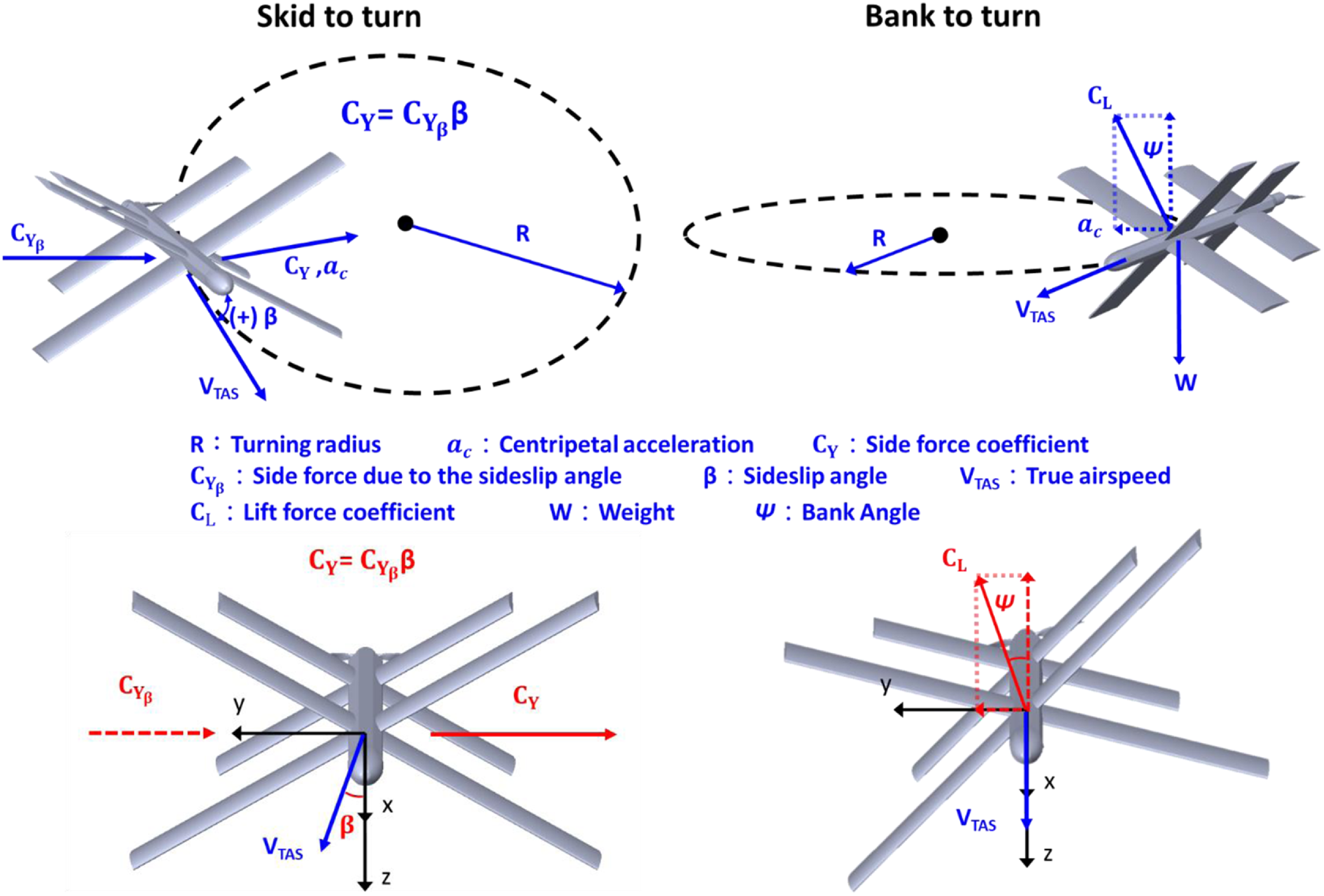
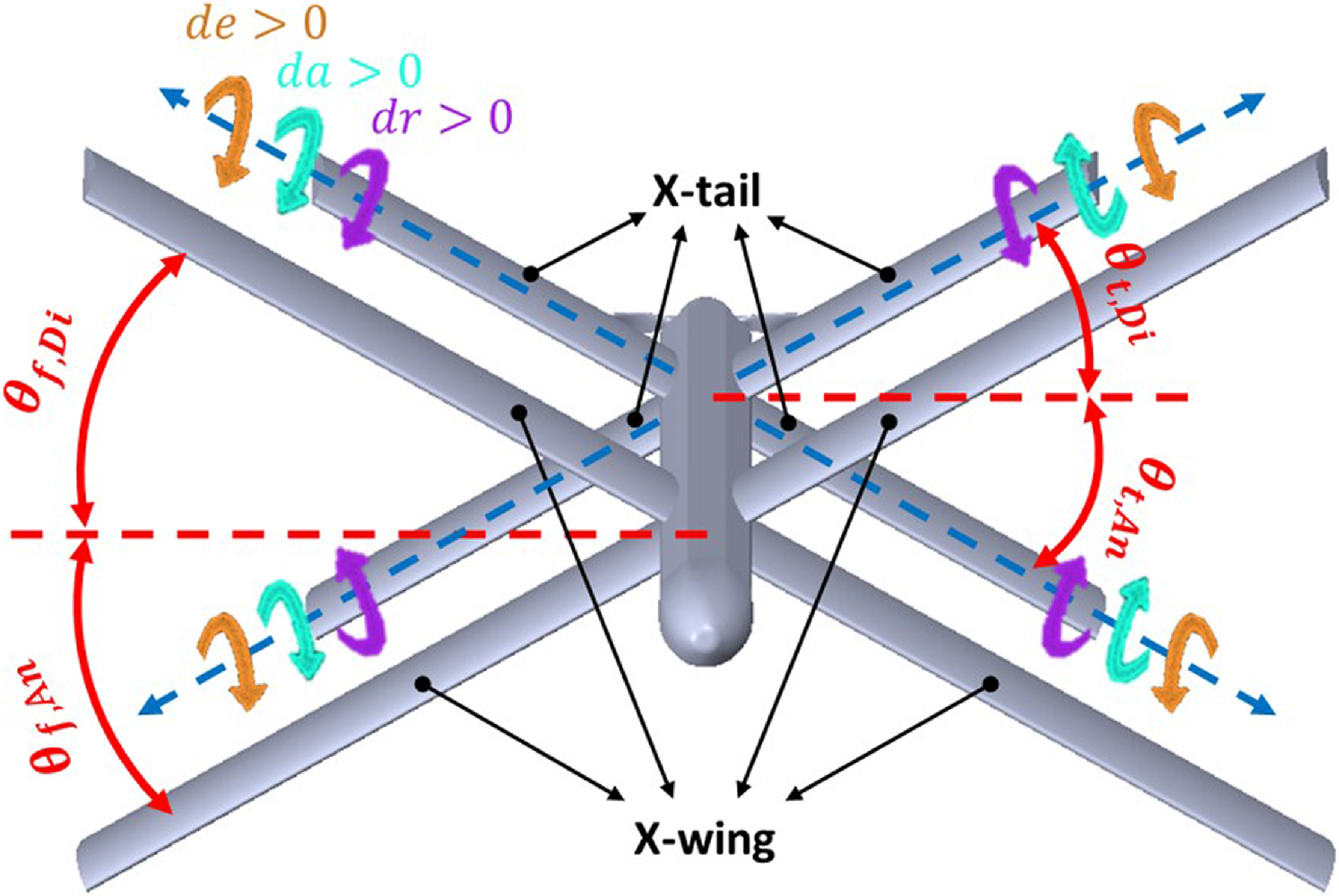
 θf,Di
 θf,An
 θt,Di
 θt,An
 dr
 da
 de
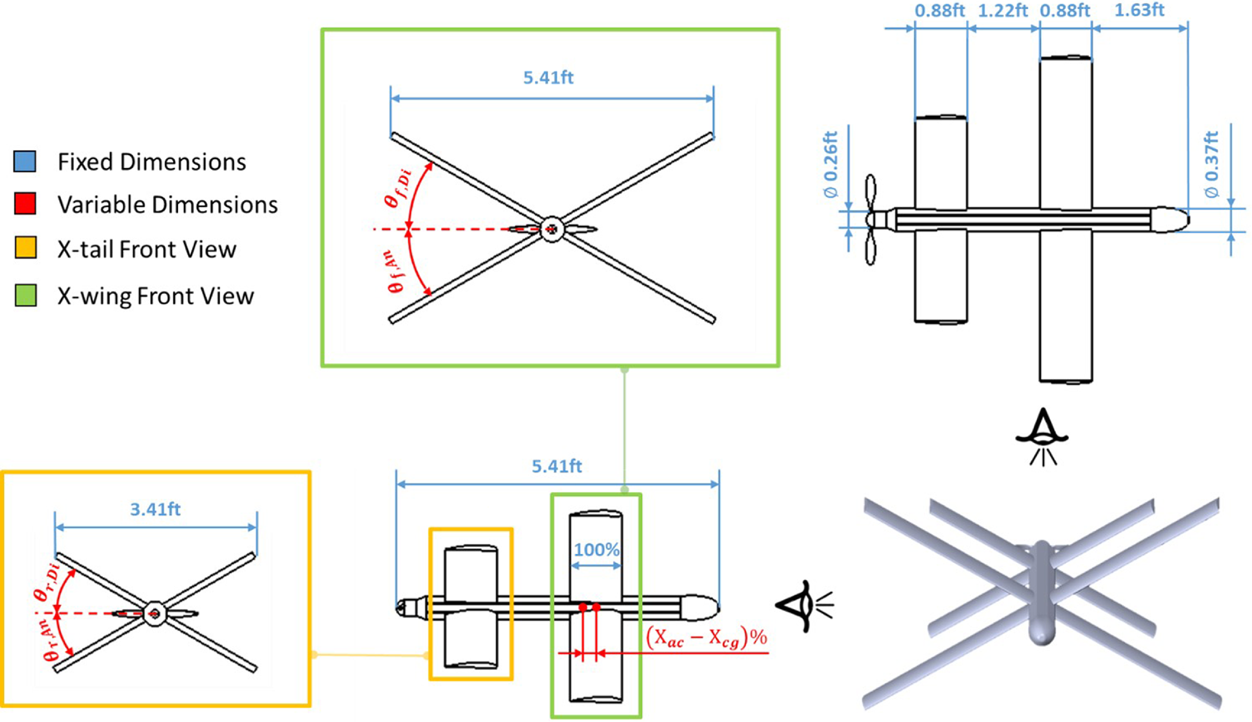
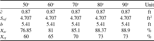
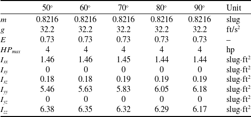
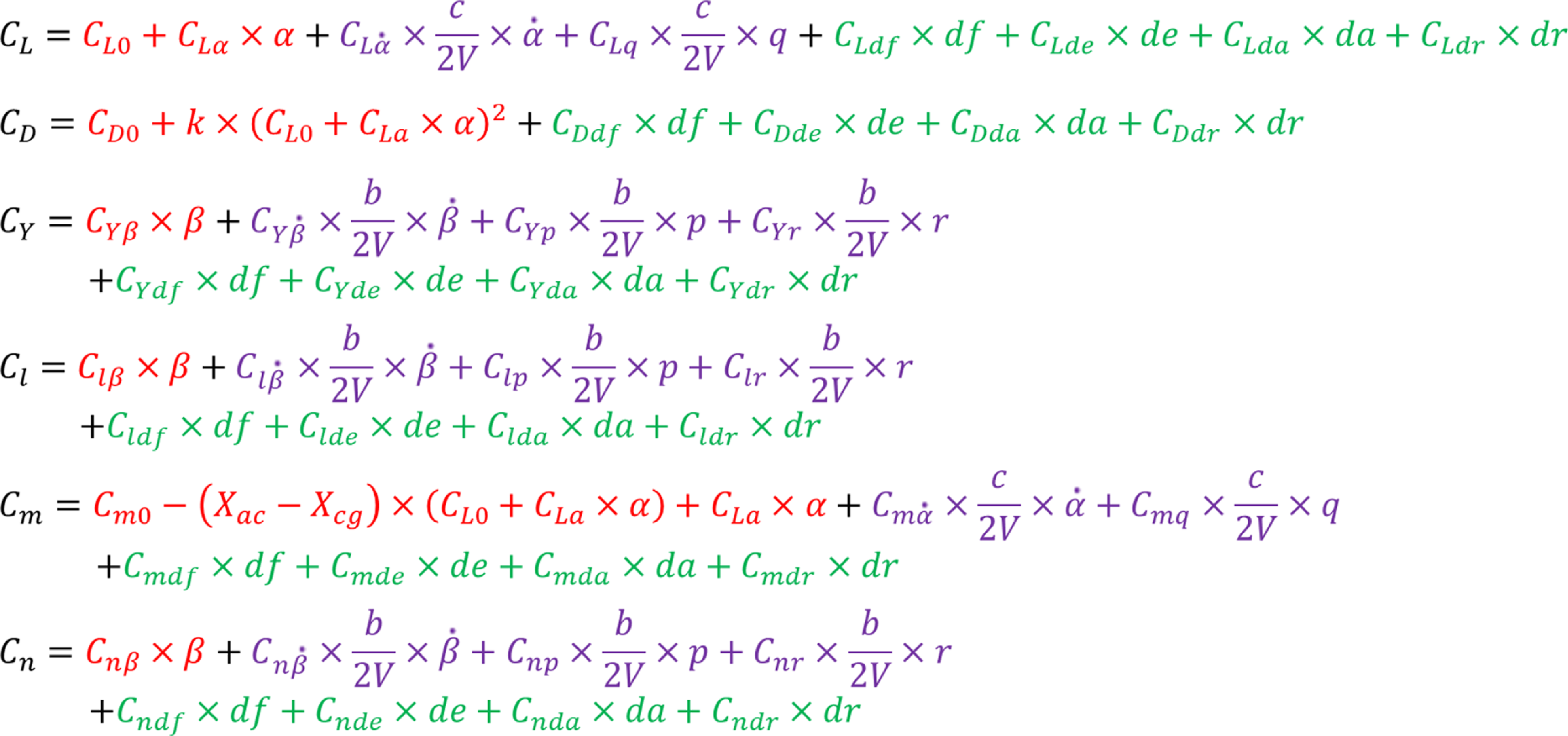
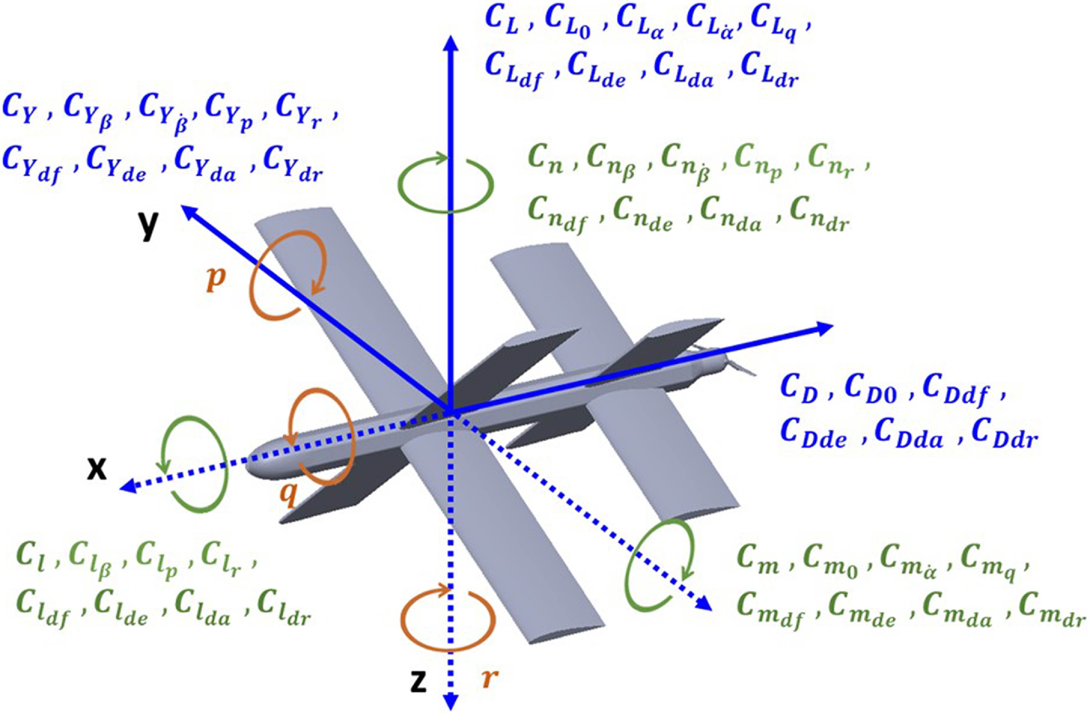
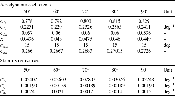
 50
 60
 70
 80
 90
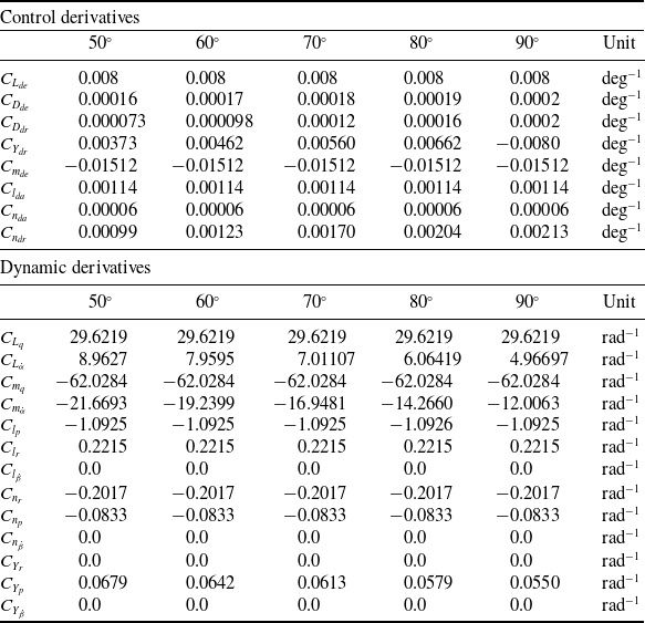
 50
 60
 70
 80
 90
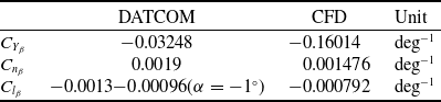
 CYβ
 Cnβ
 Clβ
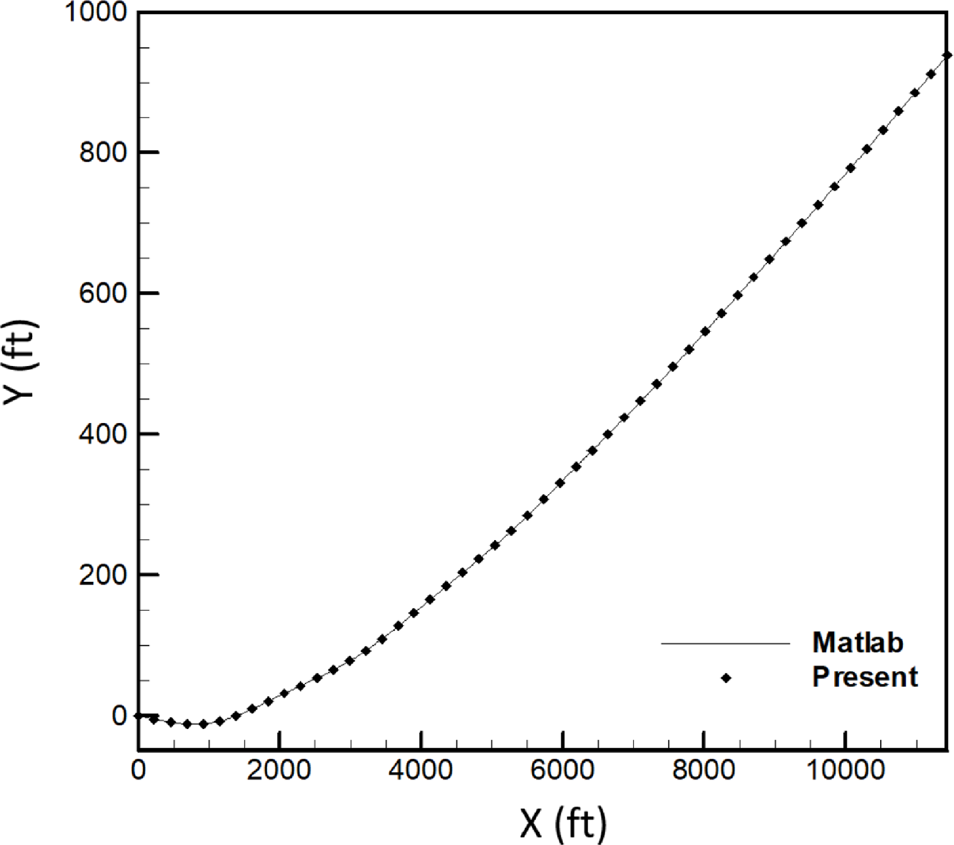
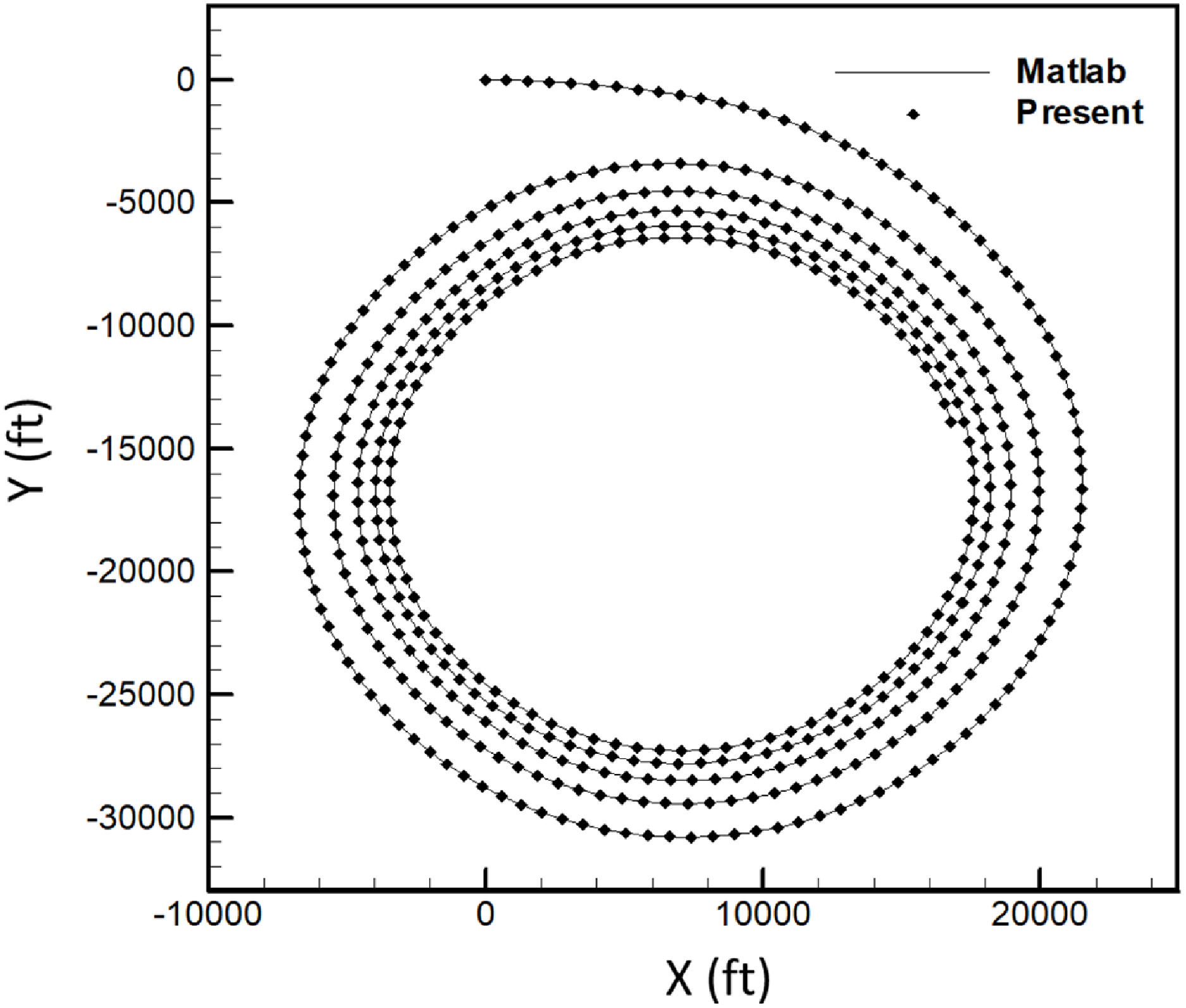
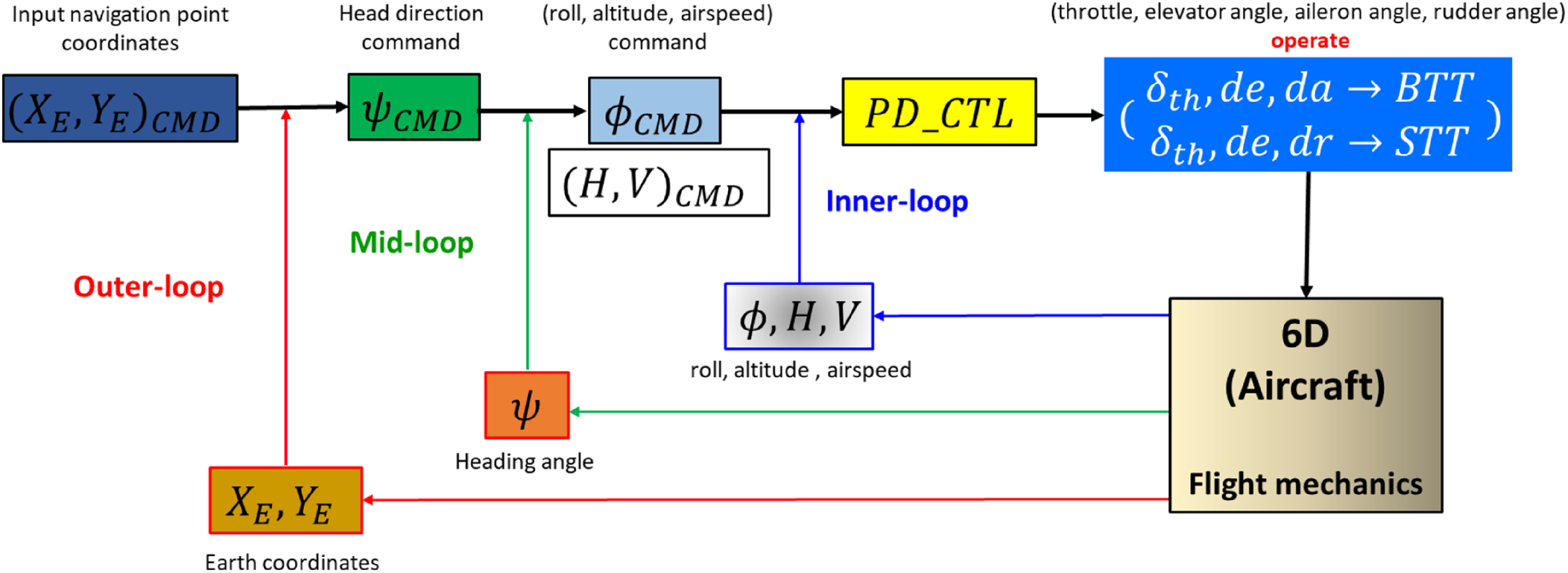
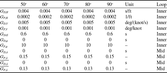
 50
 60
 70
 80
 90
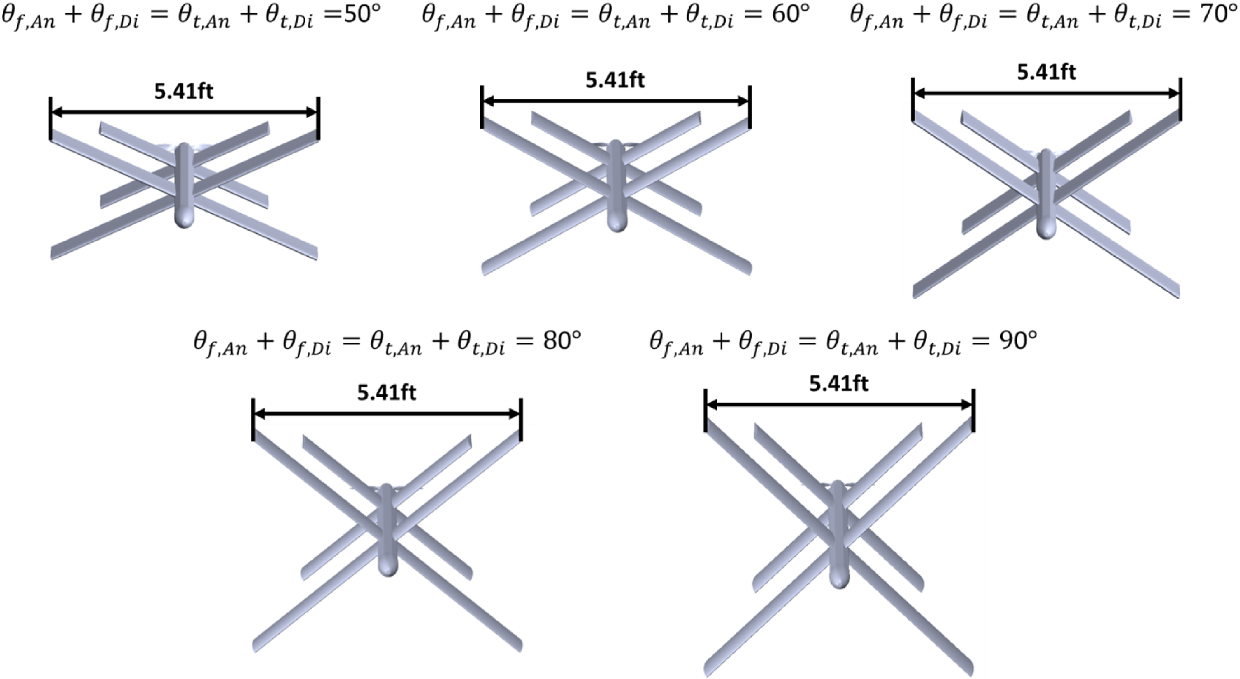
 θf,An+θf,Di=θt,An+θt,Di
 50∘
 90∘
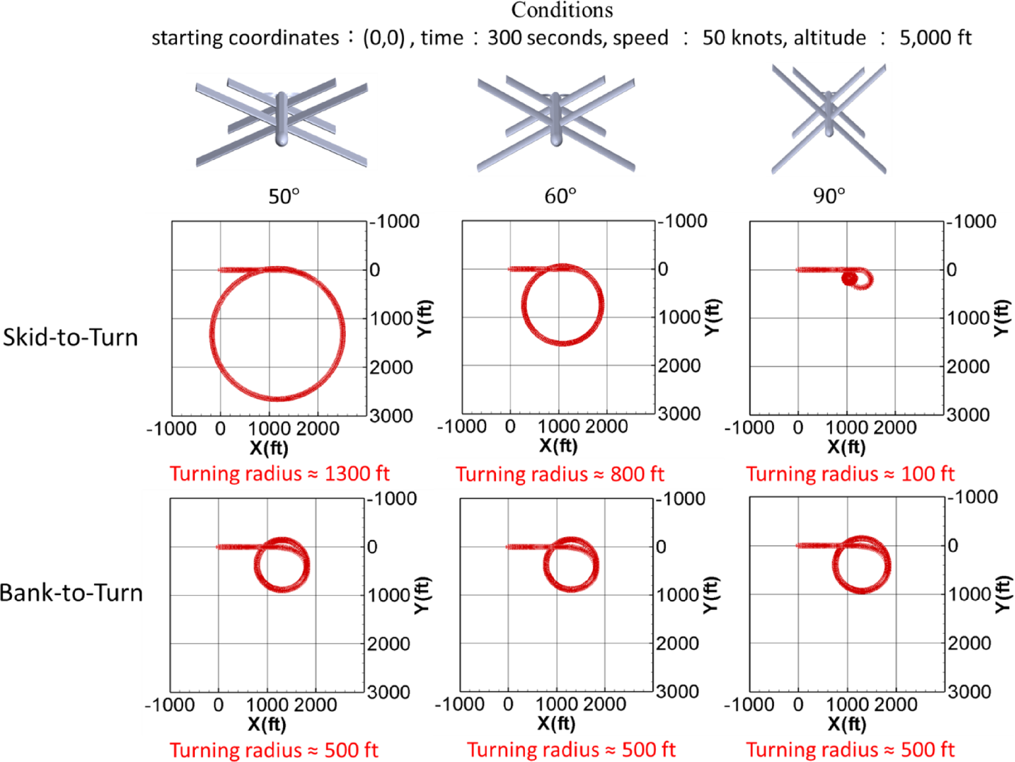
 50
 60
 90
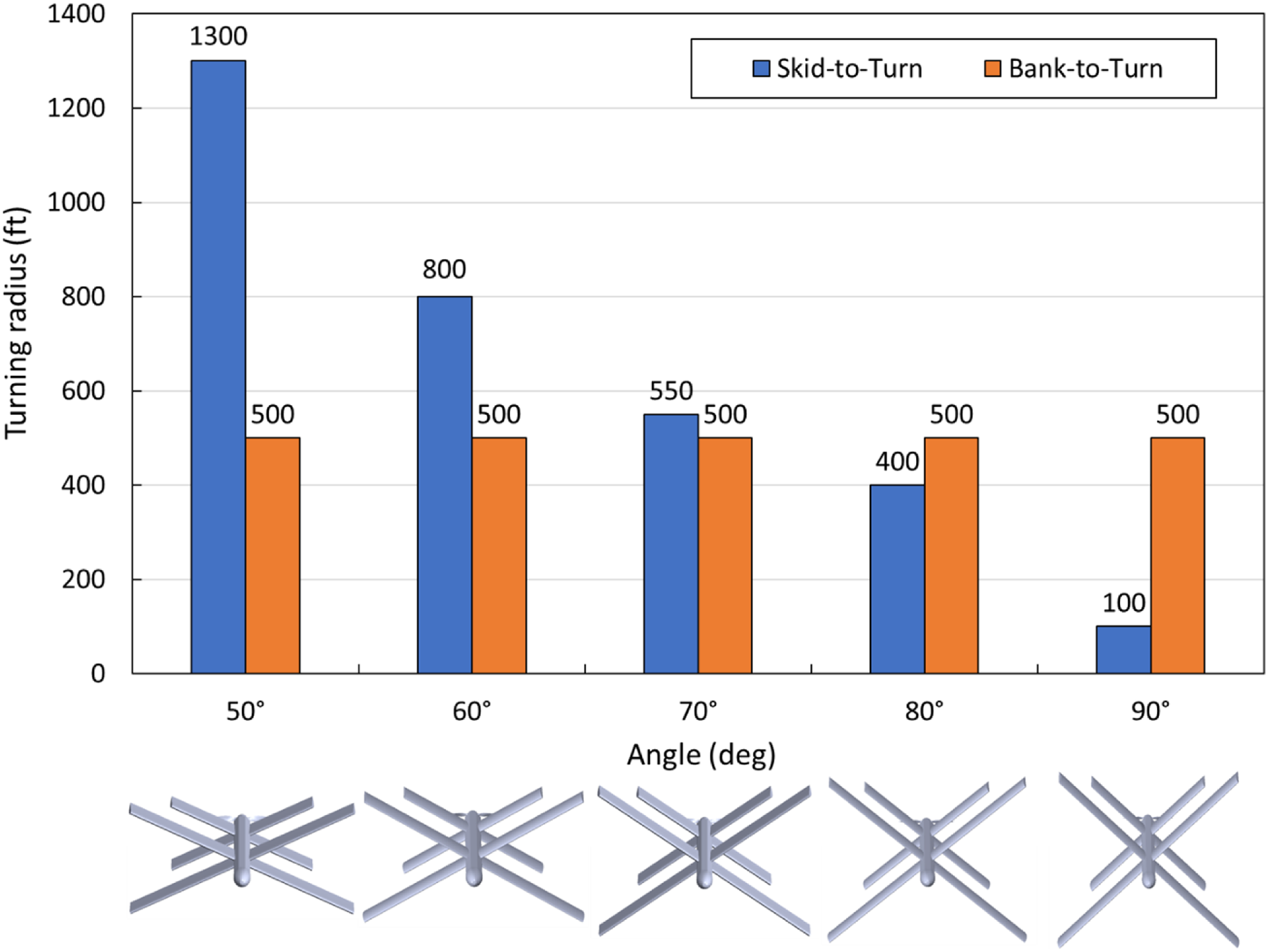
 50
 60
 70
 80
 90
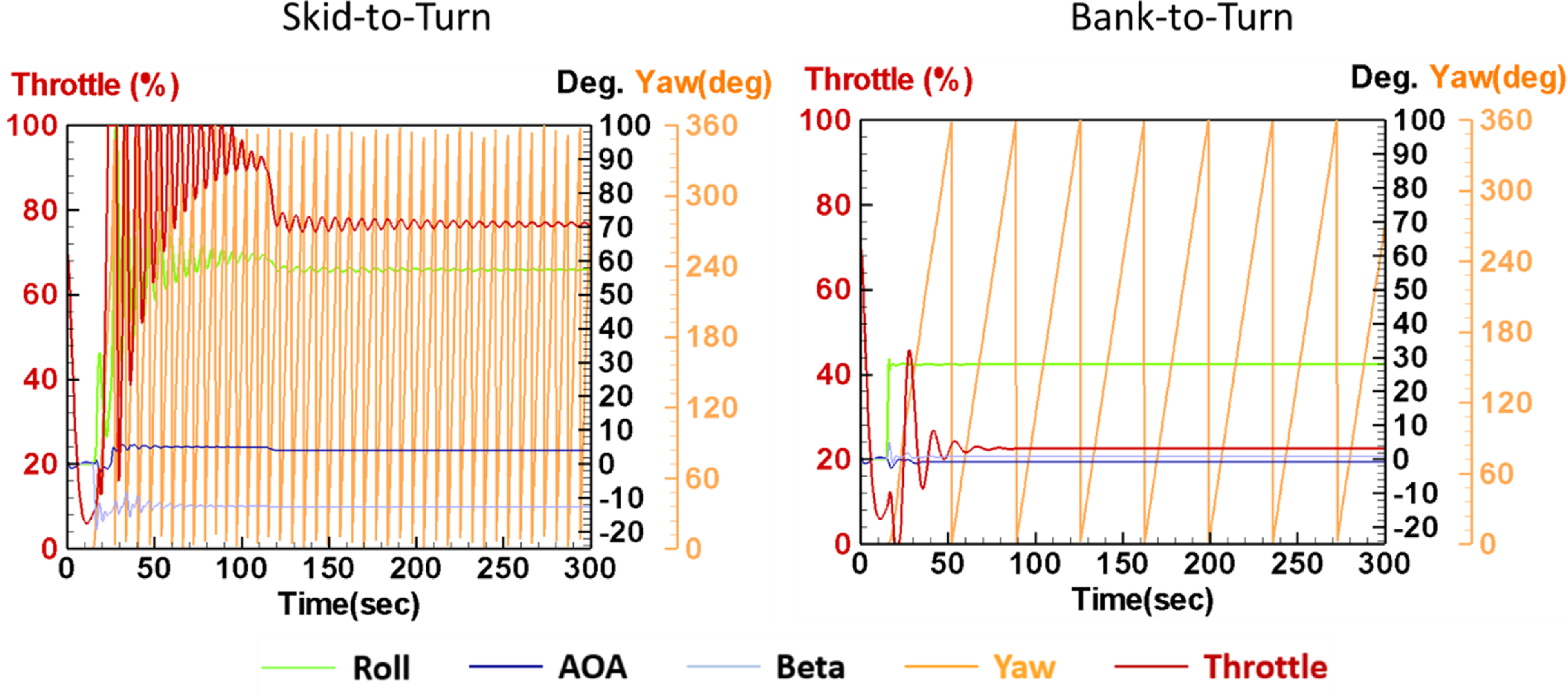
 β
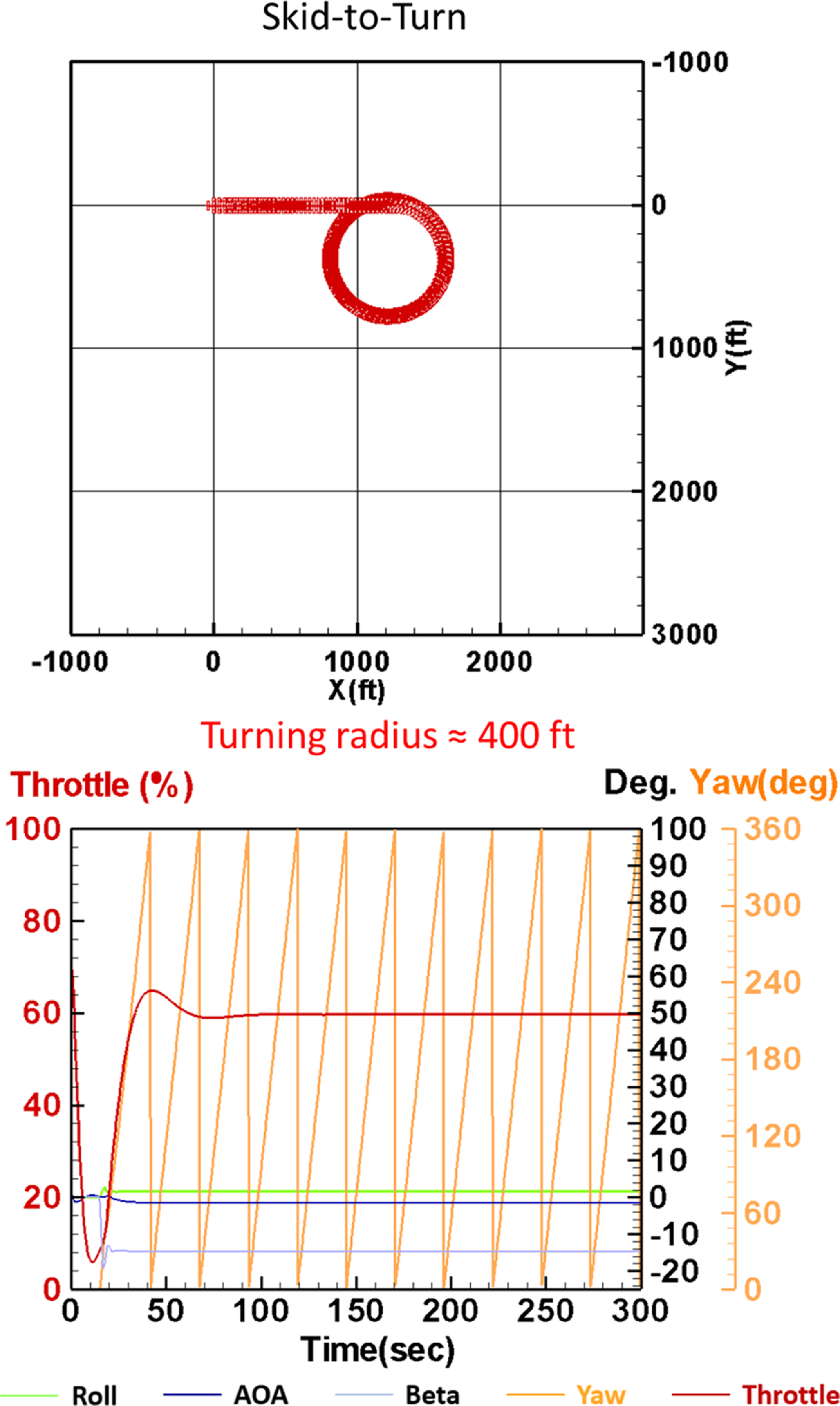
 β
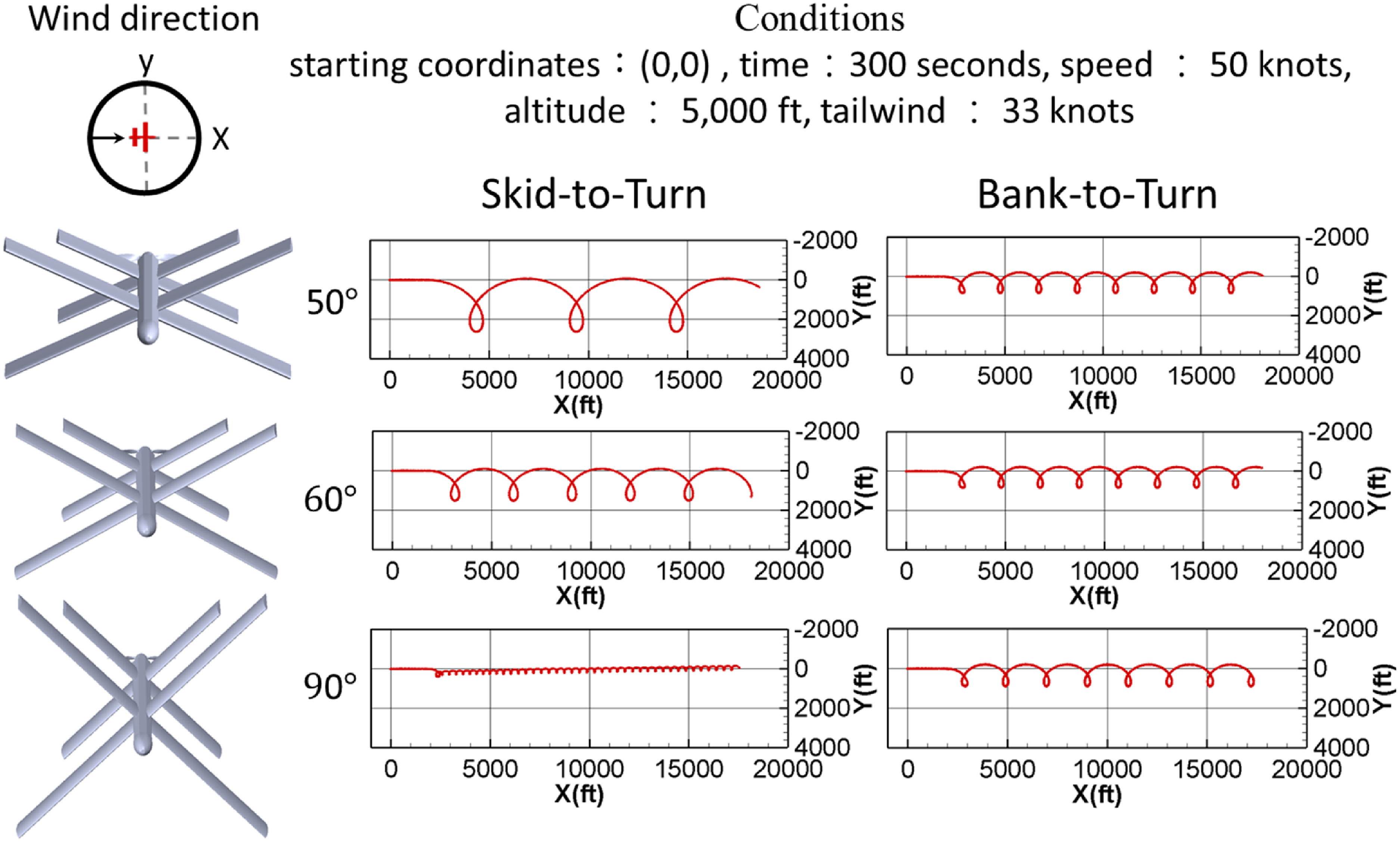
 50
 60
 90
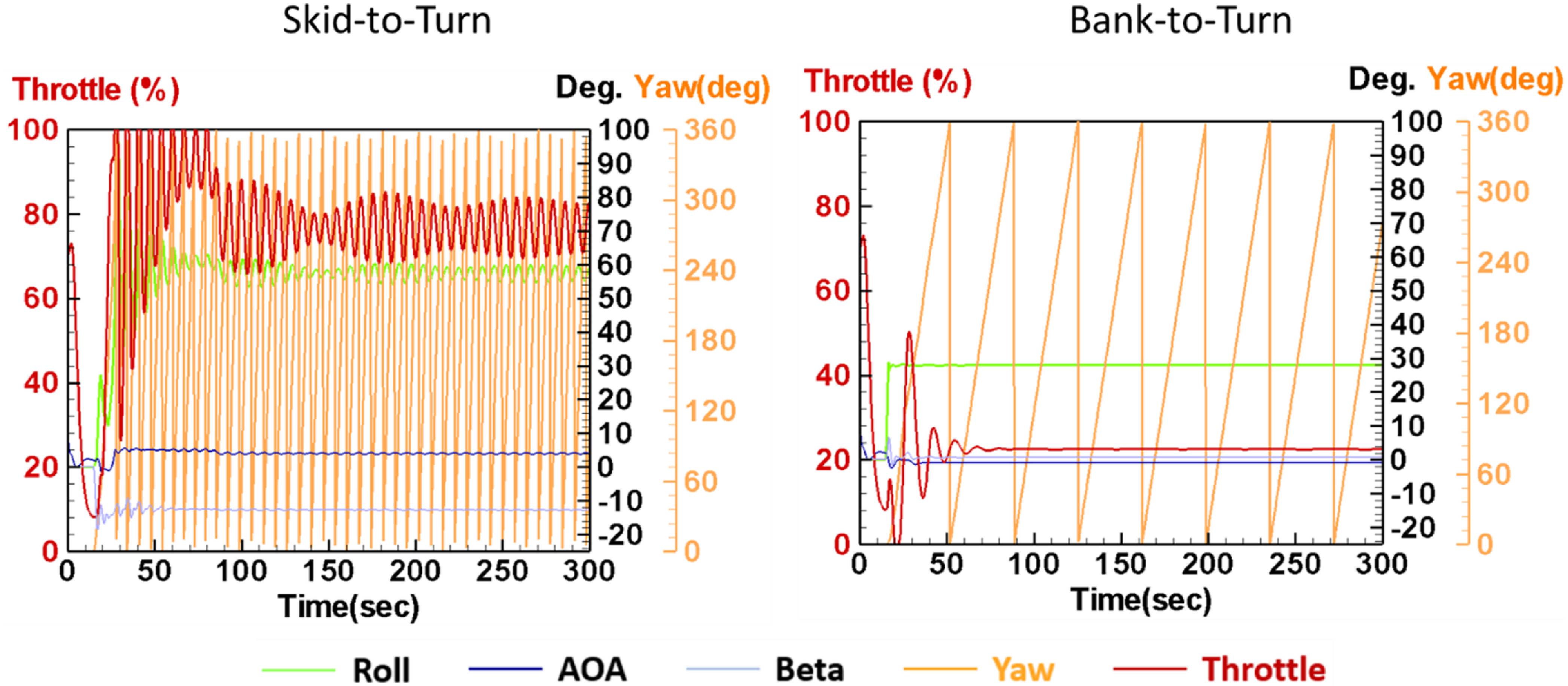
 β
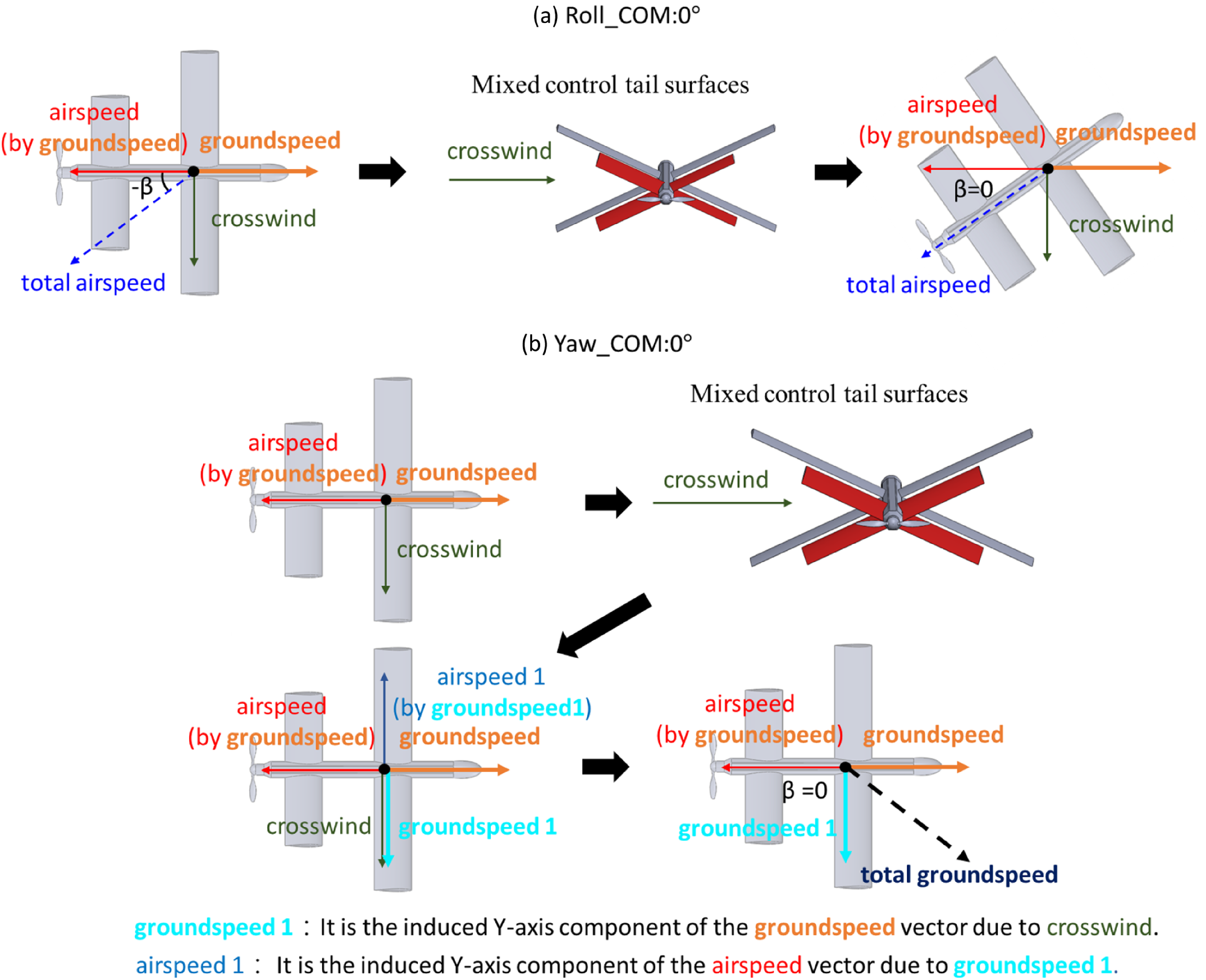
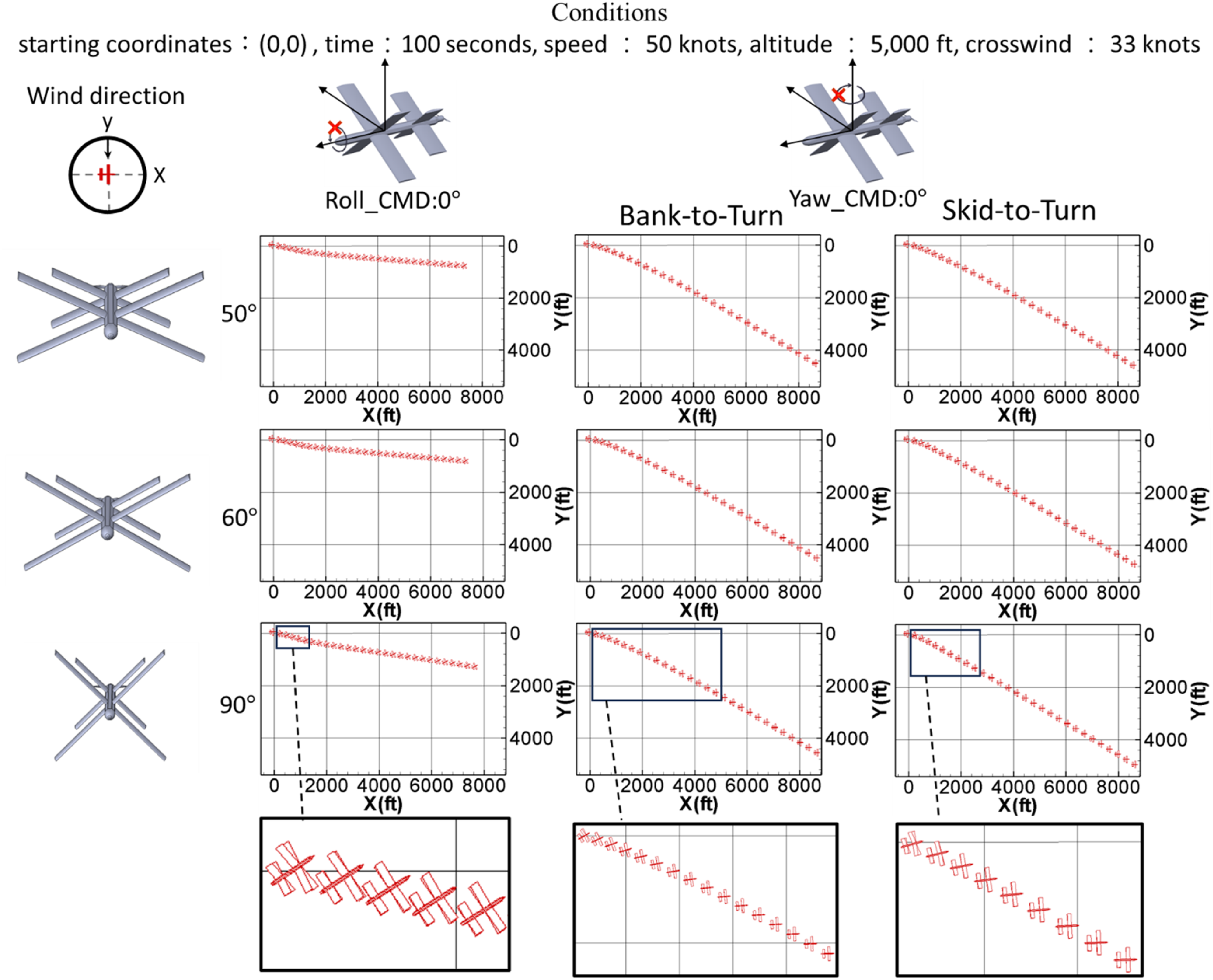
 50
 60
 90
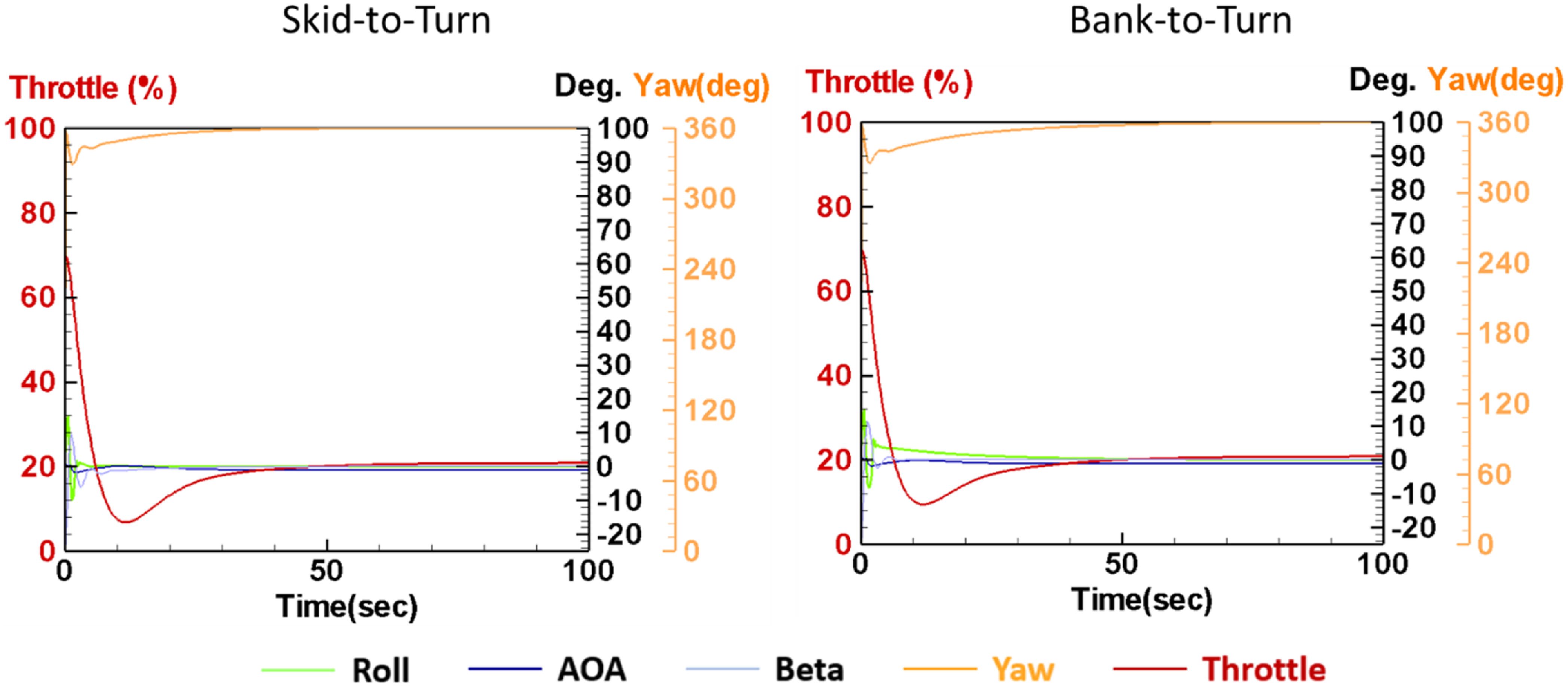
 β
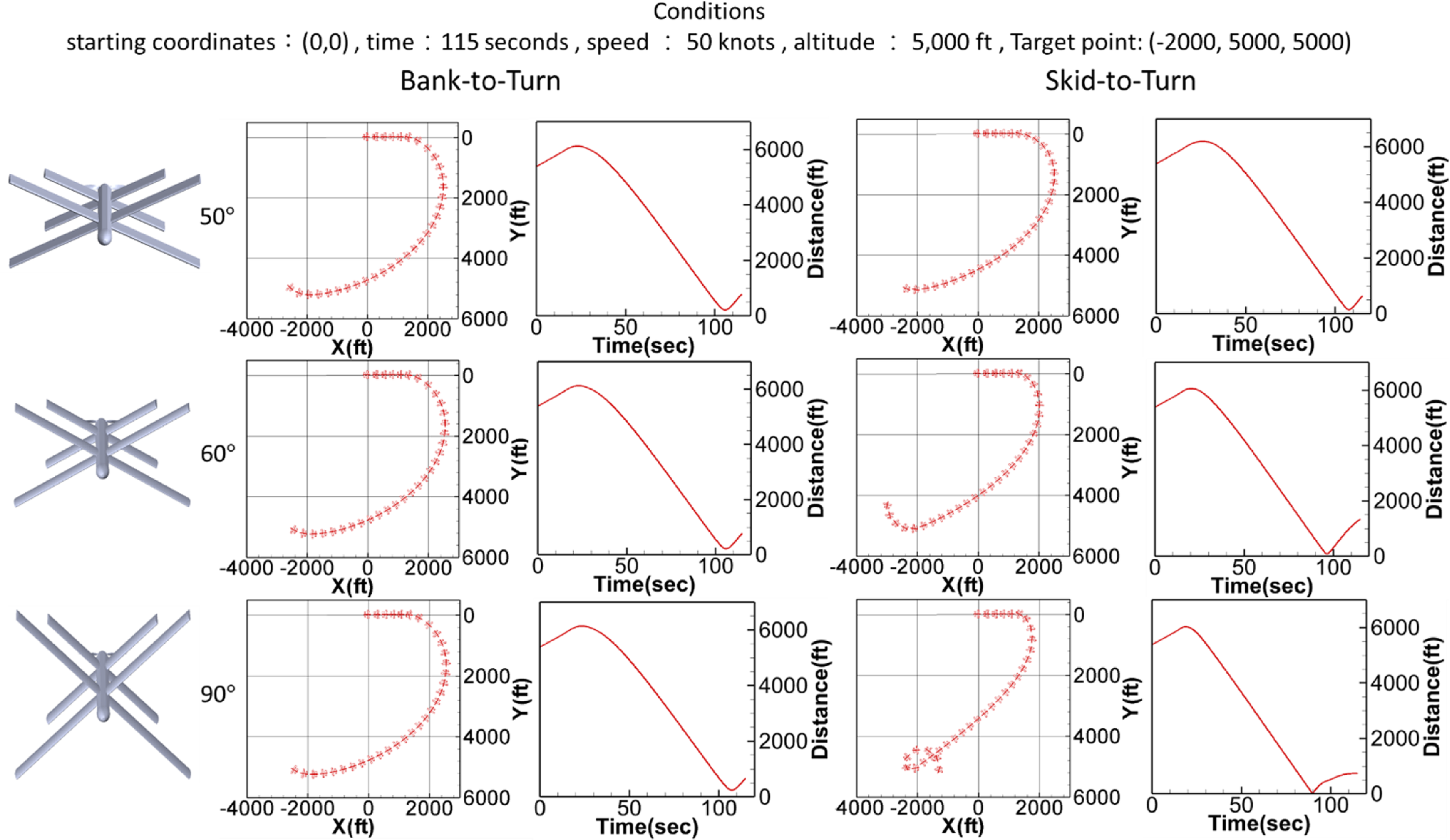
 50
 60
 90
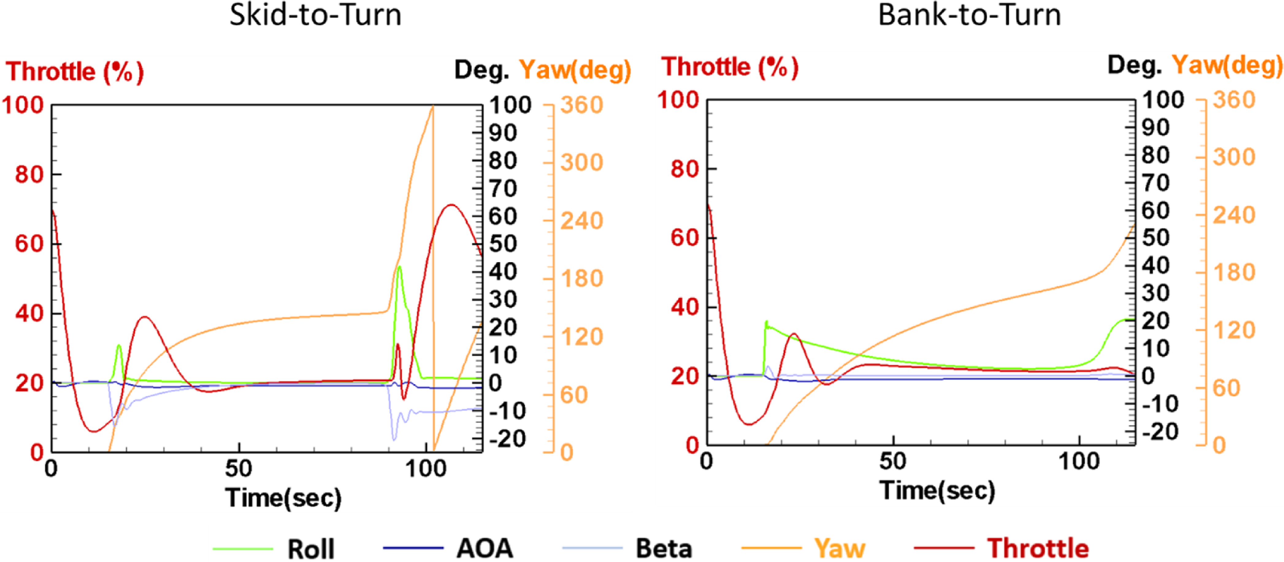
 β