2.1 Computational domain and numerical methods

Four compression ramp flows with the same angle of 30 degrees for the same Ma of 5 but different cold-wall temperatures are used to investigate the STBLI as listed in Table 1. The computational domain covered by the grid is shown in Fig. 1. Corresponding 2D auxiliary simulations are conducted to provide the inlet laminar profiles for 3D turbulent simulation. The origin of the coordinate system is set at the corner vertex. L _x1 is the streamwise length for turbulent boundary layer and L _x2 is the ramp length, L _y is the wall-normal length, L _z is the spanwise length. The specific values of these lengths are listed in Table 1. The lengths of boundary layer development, L _x1 , have been selected to try to match the Re _θ of the turbulent boundary layer for different wall temperature conditions, which will be discussed later. L _x2 have been set as 60 mm for all cases. The spanwise two-point correlations of the fluctuating velocity vectors prove that the domain spanwise scales are sufficient to solve the largest scale vortices as shown in Fig. 2.

Table 1.

Main condition parameters and computational domain sizes

Figure 1.

Computational domain and grid of STBLI. Auxiliary 2D simulations are conducted to provide laminar profiles in the inlet of the 3D simulations, and the 3D computational domain is the area covered by grids.

Figure 2.

Spanwise two-point correlations of the fluctuating velocity at (a) x = –60 mm and (b) x = 0 mm.

The governing equations are Navier-Stokes equations in curvilinear coordinate system [Reference Fu, Ma and Li13] and the boundary conditions are chosen to be comparable with the hypersonic boundary layer DNS by Duan et al. with freestream Ma of 5 [Reference Duan, Beekman and Martin14]. The compressible laminar boundary layer profiles for corresponding wall temperatures are used at the inlets to reduce computational cost, which is obtained from 2D simulations. Forced transition of boundary layers is realised by introducing blowing and suction disturbance [Reference Pirozzoli, Grasso and Gatski15, Reference Tang, Xu and Li16] to get turbulent boundary layers, which is set 20 mm behind the inlets on the wall. There is a sponge area at the outlet to prevent reflected waves. The bottom walls are no-slip and isothermal walls with different temperatures as listed in Table 1. The top is non-reflective boundary condition. The spanwise boundary condition is periodic.

The governing equations are discretised on the structural grid by the finite difference method. The first layer grid heights y ⁺ all are around 0.35 and the maximum y ⁺ downstream of the corner are controlled to around 0.6 as listed in Table 2. The maximum grid number reaches 4.16 × 108 of case T02. As the wall temperature increases, the wall viscous scale increases and hence the total grid number can be reduced to achieve the same accuracy. The grids are proved sufficient to solve turbulence, which will be discussed carefully in next subsection. Convection terms are solved by a hybrid scheme which is composed of a seven-order low dissipation upwind scheme in smooth region, a seven-order WENO scheme in non-smooth region and a five-order WENO scheme in extremely non-smooth region. Time stepping is conducted by the third-order Runge-Kutta method. Generally, the time step required for the numerical stability is much shorter than that required for the turbulence time scale, especially for high-order numerical schemes. Therefore, the time steps have been carefully selected based on Courant number and pilot calculation. The computations were performed on the open source code OpenCFD-SC, which has been widely validated by the development team for supersonic turbulence simulations [Reference Tong, Yuan and Lai17–Reference Li, Fu and Ma19] and aerodynamic heat simulations [Reference Tang, Xu and Li16].

Table 2.

Computational grid and time step setups for the DNS of STBLI for different wall temperature conditions (Note: reference location is at x = –60 mm. ${{\rm{L}}_{{\rm{ref}}}} = 1{\rm{\;mm}}$ )

The flows are steady on average and hence sampling statistics are conducted. The sampling time duration is listed in Table 2, which has been checked to be enough to ensure time convergence for first order, second order and wall gradient statistics. Particularly, this study statistically calculated all items in the heat transport equation, Equation (1), during the calculation process to explore the mechanisms of wall temperature effects on aerodynamic heat generation and transport in STBLI. Note that $\bar x$ means Reynolds average, while $\tilde x$ means Favre average, x’ and x” mean the corresponding fluctuation.

(1) \begin{align} \frac{{\partial \bar \rho {{\tilde u}_j}\tilde h}}{{\partial {x_j}}} + \frac{{\partial \bar \rho \widetilde {u_j^{{\rm{''}}}h{\rm{''}}}}}{{\partial {x_j}}} + \frac{\partial }{{\partial {x_j}}}\left( { - \lambda \frac{{\partial \bar T}}{{\partial {x_j}}}} \right) = {\bar u_J}\frac{{\partial \bar p}}{{\partial {x_j}}} + \overline {{u_j}{\rm{'}}\frac{{\partial p'}}{{\partial {x_j}}}} + 2\mu \overline {S_{ij}^d} \overline {S_{ij}^d} + 2\mu \overline {S_{ij}^d{\rm{'}}S_{ij}^d{\rm{'}}} \end{align}

2.2 Grid with independence test

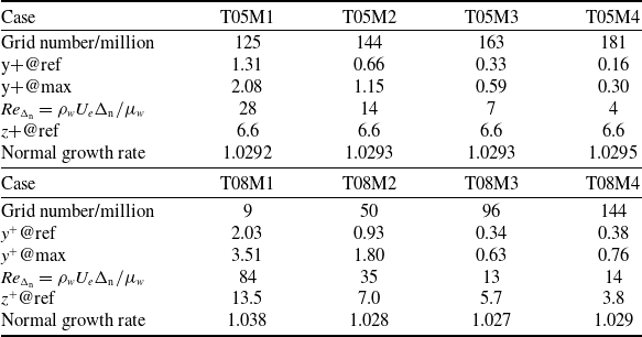
Grid quality largely influences DNS quality and the near-wall grid largely influences the wall gradients like wall frictions and wall heat fluxes. Taking cases T05 and T08 as examples, two grid independence tests were conducted with eight sets of grids as shown in Table 3. For case T05, the total grid number varies from 1.25 × 10⁸ to 1.81 × 10⁸ and for case T08 varies in a larger range from 9 × 10⁶ to 1.44 × 10⁸. The tests mainly focus on the independence of normal grids, which is important for the present research purpose, i.e. calculation of wall shear stresses and wall heat fluxes. The wall normal grid Reynolds number $R{e_\Delta }_n$ is also given to estimate the grid quality in the table, which is suggested around 10 generally and can be relaxed to even 40 for low-dissipation numerical schemes [Reference Ma and Liu20]. The normal growth rates of all cases are kept close while the wall-normal grid number varies.

Table 3.

Grid setup for the independence test of case T05 and case T08 (The cases are named by the basic case of different wall temperature conditions)

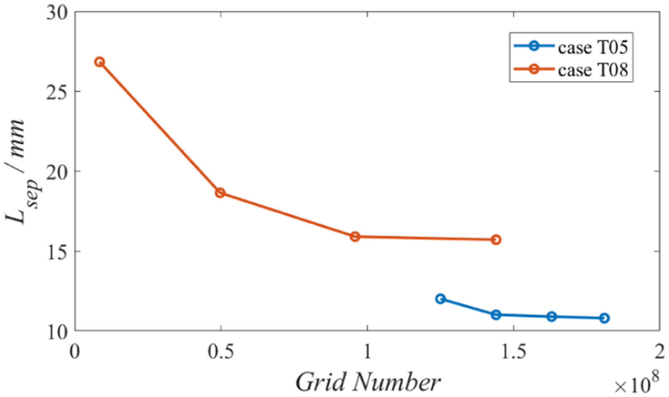
The separation lengths around the corner are used to determine the grid independency as shown in Fig. 3. The results show that the separation length decreases as the total grid number increases. Cases T05M3 and T08M3 both reach grid independency.

Figure 3.

Grid convergence of the separation length in STBLI for case T05 and case T08.

Figure 4.

Wall pressure coefficient (a and c) and friction coefficient distribution (b and d) computed by different grids for case T05 and case T08.

The wall pressure and skin friction distribution are further investigated to confirm the grid independency, and the results are given in Fig. 4. It can be seen that the wall pressure distribution is insensitive to the grid, which further indicates that the interaction length is also insensitive to the grid. For the skin friction coefficient, the upstream area reaches grid convergence while the grid has great influence on the wall friction downstream of the corner. Case T05M3 shows good grid convergence downstream of STBLI as shown in Fig. 4(b). Case T08M3 basically reaches grid independence with acceptable error. Above all, the grid-independent case T05M3 and T08M3 will be used to analyse wall temperature effects on aerodynamic heating mechanisms.

2.3 Characteristics of incoming boundary layer and validation

The states of incoming boundary layer have great effects on STBLI and hence they are investigated first. The boundary layer characteristics at the reference station (x = −60 mm) are provided in Table 4, including boundary layer thickness, profile factors, some common-use Reynolds numbers, skin friction coefficients and Stanton numbers. The nominal thickness δ will be used to nondimensionalise length quantity, and the displacement thickness δ ^* will be used to predict the interaction length. The profile factor H decreases as the walls are cooled, which indicates that the velocity profiles become fuller for colder wall temperatures. $R{e_\theta }$ for all cases are kept close around 4,000 to weaken the effect of incoming turbulent boundary layer states on the STBLI so that the wall temperature effects can be investigated more dependently. $R{e_\tau }$ , which is defined as ${\rho _w}{u_\tau }\delta /{\mu _w}$ , varies between different temperature cases because the fluid properties on the wall strongly depend on the wall temperature. Recently a more appropriate friction Reynolds number $Re_\tau ^*$ was proposed by Trettel et al. [Reference Trettel and Larsson21], which is based on mainstream fluid properties and defined as ${\rho _\infty }{\left( {{\tau _w}/{\rho _\infty }\;} \right)^{\frac{1}{2}\;}}\delta /{\mu _\infty }$ . The result shows that $Re_\tau ^*$ of different cases are also close as listed in Table 4. ${C_f}$ and $\;St$ results indicate that cold walls increase the skin friction and heat transfer of the incoming turbulent boundary layers. The Reynolds analogy factors are around 1.1 and slightly increase with wall temperature decreasing, which is consistent with the study of Duan et al. [Reference Duan, Beekman and Martin14].

Table 4.

Characteristic parameters of the undisturbed turbulent boundary layers at the reference position

Figure 5.

Turbulent boundary velocity profiles at the reference station after (a) van Driest transformation [Reference van Driest22] and (b) Trettel-Larsson transformation [Reference Trettel and Larsson21].

Velocity profiles and temperature profiles of the undisturbed turbulent boundary layer at the reference station are further validated by comparing with some previous theories. The van Driest transformation [Reference van Driest22] of velocity profiles are provided in Fig. 5(a) with the wall law of incompressible boundary layers. The results show that the profile of adiabatic wall collapses well with the wall law of incompressible turbulent boundary layers. All velocity profiles show notable linear and logarithmic region but with some difference in detail. The linear region in the viscous sublayer is small for cold walls, especially for case T02, which can be explained by the decreased molecular viscosity and small viscosity-dominated region. In addition, the wake layer is higher for colder wall conditions. After considering the influence of wall temperatures, the Trettel-Larsson transformation velocity profiles [Reference Trettel and Larsson21] are calculated and show better agreement with the wall law for all wall temperature cases, as shown in Fig. 5(b), except for the slight deviation of case T02 wake layer. The deviation is caused by the limitation of the present computational domain of case T02, leading to the influence of the inlet Mach wave, which goes through the profiles at the reference station (x = −60 mm) as clearly shown in Fig. 7. Fortunately, the inlet Mach wave does not influence STBLI around the corner.

The velocity-temperature relationship is also important in a compressible boundary layer. The DNS results are compared with Walz relationship [Reference Walz23] as shown in Fig. 6(a), showing that the adiabatic case collapse with Walz theory, but cold-wall cases deviate from Walz theory. The deviation can be attributed to the failure of the strong Reynolds analogy in non-adiabatic cases. Recently, Zhang et al. [Reference Zhang, Bi, Hussain and She24] proposed a generalised relation, which considers wall heat transfer effects. The results given in Fig. 6(b) shown that the corrected prediction of Zhang’s relation are in great agreement with the present DNSs. Compared with previous DNS results of Duan et al. [Reference Duan, Beekman and Martin14] and Chu et al. [Reference Chu, Zhuang and Lu25], they have similar boundary conditions with the present DNS. The Mach number in Duan et al.’s case is 4.97 while Chu et al.’s case is 4.9, and the Tw/Tr in Duan et al.’s case is 0.54 while Chu et al.’s case is 0.50. The results show that there are some minor deviations mainly near the wall compared with Duan et al.’s results and the present DNS profile is closer to that of Chu et al., which is because the wall temperature of the present DNS is closer to that of Chu et al. On the whole, the temperature results of the present DNS is accurate and reliable.

Figure 6.

Velocity and temperature relations of incoming turbulent boundary velocity profile at the reference station (solid lines) compared with (a) Walz relation theory (dash lines) [Reference Walz23], (b) Zhang relation theory (dash lines) [Reference Zhang, Bi, Hussain and She24] and previous DNS data of Duan et al. [Reference Duan, Beekman and Martin14] and Chu et al. [Reference Chu, Zhuang and Lu25].

In conclusion, the results of turbulent boundary layer proved the reliability of the wall temperature effects on the calculation results.

3.1 Instantaneous and averaged flow structures

The instantaneous flow fields of the whole computational domains are shown in Fig. 7. The results indicate that the boundary layer transition is advanced with the decrease of wall temperature and for this reason the streamwise length of case T02 domain has been reduced to control the development degree of turbulent boundary layer and hence control the $R{e_\theta }$ . In the upstream undisturbed turbulent boundary layer, the coherent structures at the edge of the boundary layer induce small shocklets in the mainstream, indicating that the fluctuating Mach number exceeds 1 at the edge of the boundary layer. In the interaction region, the separation zones shrink as the wall temperature decreases. The turbulent coherent structures cause the fluctuating of shock waves when passing through the shock waves, and the fluctuation decreases with the decrease of the wall temperature.

Figure 7.

Transition process of turbulent boundary layer and instantaneous flow fields of STBLI for different wall temperatures.

From the x-z plane, the instantaneous flow fields show some interesting structures and the wall temperature effects are significant as shown in the slices of ${y^ + } = 10$ in Fig. 8. In the upstream undisturbed turbulent boundary layer, there exist typical velocity streaks, and the spacing between the adjacent streaks all are about 200 ${\delta _\nu }$ for all wall temperature cases. As the wall temperatures decrease, the streaks become more straight and well-organised. In the interaction region, there exist irregular and turbulent separation zones. Interestingly, the separation zones are not continuous in the spanwise direction but show some large-scale spanwise periodicity; for example, there exist two separation bubbles in spanwise direction for case T10. It can be seen more clearly that the separation zones decrease as the wall temperatures decrease. Downstream of the reattachment lines, some large-scale streaks appear, which were explained by the Gortler instability in previous literature [Reference Simeonides and Haase26–Reference Navarro-Martinez and Tutty28]. As the wall temperature decreases, the large-scale streaks also become straighter.

Figure 8.

Wall temperature effects on high-speed velocity streaks in near-wall viscous sublayer. The slice heights ${{\rm{y}}^ + } = 10$ for all cases.

The turbulent results have been averaged over time and spanwise direction, and the average flow fields are provided in Fig. 9. The results show that wall temperatures have little effect on the mainstream shock wave but great effect on the separation bubbles around the corner. As the wall temperature decreases, the shock feet around the corner become straighter and closer to inviscid ideal shock waves. The average separation bubbles of the four cases are extracted from the mean flow field for comparison in Fig. 9(e). The bubbles are both flat and close to triangle shapes. As the wall temperature decreases, the bubble shrinks and the recirculation centre moves toward the wall.

Figure 9.

Wall temperature effects on the average flow fields (a–d) and recirculation bubbles (e). The white dash lines represent inviscid shock waves and the streamlines represent boundary layer edges in (a)–(d). The corresponding points represent the recirculation centres in (e).

3.2 Separation lengths and upstream interaction lengths

According to the skin friction distribution, the separation lengths are further obtained for different wall temperatures and power fitting results are provided as shown in Fig. 10. In upstream undisturbed turbulent boundary layers, the skin friction coefficients decrease slowly for all cases, and case T02 gives the maximum skin friction coefficient. Around the corner, the skin friction coefficients decrease dramatically and go below zero, which indicates the occurrence of the separations. Downstream of the corner, the skin friction coefficients increase with the recovery of the boundary layers and go above zero, which indicates the reattachment. Coincidentally, all cases recover to the same peak downstream. The separation lengths are further obtained and fitted by linear law proposed by Spaid et al. [Reference Spaid and Frishett29] and power law of 0.85 proposed by Zhu et al. [Reference Zhu, Yu and Tong3] as shown in Fig. 10(b). The results show that the linear fitting is a simple but acceptable approximation, which can be expressed as the following formula [Reference Spaid and Frishett29]:

(2) \begin{align}\frac{{{L_{sep}}}}{\delta } = 2.9\left( {\frac{{{T_w}}}{{{T_r}}} - 0.08} \right) . \end{align}

Figure 10.

Friction coefficient distribution (a) and quantitative fitting of the separation lengths (b) for different wall temperatures.

However, the theory of Zhu et al. [Reference Zhu, Yu and Tong3] deviates from the present results, which imply that the exponent is 0.85. The present power fitting gives that:

(3) \begin{align} \frac{{{L_{sep}}}}{\delta } = 2.8{\left( {\frac{{{T_w}}}{{{T_r}}}} \right)^{1.45}} . \end{align}

There is an essential difference between the exponent above 1 and below 1. The deviation of Zhu’s power theory [Reference Delery2] may be attributed to their neglect to consider the extreme cold wall condition for which the separation length will shrink more slowly, resulting in an exponent greater than 1.

According to the wall pressure distribution, the upstream interaction lengths are investigated for different wall temperatures. As shown in Fig. 11, the wall pressure ratios increase more sharply for lower wall temperature, but all basically reach the inviscid theoretical value downstream of the corner. An interesting point is that all the pressure rise curves for different wall temperatures pass through the same point near the corner vertex as shown in Fig. 11. According to Chapman’s free interaction theory [Reference Chapman, Kuhen and Larson30], the upstream pressure rise is not affected by the downstream, based on which the platform pressures are predicted to be about 3.55∼3.76 for present wall temperatures, which is close to the pressure ratio at the intersection point. Furthermore, the interaction scales, which are defined as the distance between the initial rise points of the wall pressure and the vertices of the compression corner, are calculated and nondimensionalised by the method of references [Reference Souverein, Bakker and Dupont8, Reference Jaunet, Debieve and Dupont9]. As shown in Fig. 12, the maximum relative deviation between the results and the Souverein’s correlation ( ${L^*} = 1.3S_{e}^{*3}$ ) is 25%. Reference data have also been collected and presented in Fig. 12, including the adiabatic results compiled by Souverein et al. [Reference Souverein, Bakker and Dupont8] and some recent non-adiabatic results from Jaunet et al. [Reference Jaunet, Debieve and Dupont9], Spaid & Frishett [Reference Spaid and Frishett29], Schreyer et al. [Reference Schreyer, Sahoo, Williams and Smits31], Bhagwandin et al. [Reference Bhagwandin, Helm and Martin32], Volpiani et al. [Reference Volpiani, Bernardini and Larsson7] and Zuo et al. [Reference Zuo, Wei and Hu10]. The results, especially non-adiabatic results, are around the fitting lines and hence basically verifies the wall-temperature-corrected theory proposed by Jaunet et al. [Reference Jaunet, Debieve and Dupont9].

Figure 11.

Wall temperature effects on wall pressure distribution. The subscript u means the value at the undisturbed reference position (x = −60 mm).

Figure 12.

Normalised interaction length compared with the scaling theory proposed by Souverein et al. [Reference Souverein, Bakker and Dupont8] and corrected by Jaunet et al. [Reference Jaunet, Debieve and Dupont9]. The grey symbols are from Souverein et al. 2013, for adiabatic cases; the red symbols represent hot wall conditions; the blue symbols represent cold wall conditions.

Above all, cold walls lead to more coherent turbulent structures and weaken the shock surface fluctuation. Cold walls also reduce separation lengths and the present study quantitatively suggests that there are limitations in Zhu et al.’s theory of 0.85 power relation [Reference Zhu, Yu and Tong3] between separation length and wall temperature, which is limited for extremely cold walls. For extremely cold walls, it seems that the separation length is proportional to the wall temperature to the power of 1.45, and hence further quantitative research is needed. Finally, the present study quantitatively validates the wall-temperature-corrected interaction scaling theory in recent literature [Reference Jaunet, Debieve and Dupont9].

4.1 Wall cooling effects on temperature field characteristics

The instantaneous hot structures in STBLI for cold walls are investigated first and case T02 is presented in Fig. 13 as a representative example. The results show that there are irregular hot fluid masses ejecting into the mainstream at the edge of the boundary layer. The enlarged image provides more details, which show that in the extreme near-wall area, the high-temperature fluid gathers at a height away from the wall and the edge of the high-temperature fluid near the wall is a relatively regular wave shape. In the interaction region, the shock angle is larger where the high-temperature fluid passes through. The extremely high-temperature fluid appears on the ramp, which is distributed at the bottom of the boundary layer and near the shock wave. These high-temperature fluid brings intense aerodynamic heat to the walls.

Figure 13.

Instantaneous hot structures in the temperature field of STBLI for cold wall conditions, taking case T02 as an example.

Figure 14.

The averaged temperature profiles at six representative streamwise locations. (x_r, y_r) is the ramp coordinate and T₂/T₁ is the theoretical temperature ratio behind the oblique shocks. Upstream undisturbed turbulent boundary layer (a); the separation point in case T10 (b); the separation point in case T02 (c); the reattachment point in case T10 (d); downstream boundary layer in the recovery process (e and f).

The temperature fields are averaged over time and spanwise direction and the averaged temperature profiles at six representative streamwise locations for all the wall temperatures are provided in Fig. 14. For undisturbed hypersonic turbulent boundary layer (x/δ = −6), the temperature overshoot near the wall becomes significant as the wall temperature decreases, which intuitively reflects the aerodynamic heating. Besides, it can be found that the temperature boundary layer is slightly thicker than the velocity boundary layer. When the flow separation occurs in case T10 (x/δ = −2.2), the high-temperature layer near the wall in case T10 becomes thicker while the profiles of the other three cases still are not disturbed. When the flow separation occurs in case T02 (x/δ = −0.43), the flows are all in recirculation states for the other three cases. At this station, the temperature profiles are all fuller, which indicates that the low-speed fluid is heated by aerodynamic compression. On the ramp at x _r /δ = 0.8, the near wall fluid of the case T02 is first heated to the theoretical post-shock temperature, the boundary layer is initially formed and an obvious shock wave appears. For other three cases, the boundary layers are still interacted with the shock layers intensively. At x _r /δ = 2.0, the boundary layer of the case T05 is also gradually formed, and the shock layers become thicker. At the further downstream station x _r /δ = 4.0, obvious boundary layers and shock waves are formed except for the case T10. For the case T10, the boundary layer is still in the recovery process where the near wall fluid accelerates and cools suddenly leading to the temperature profile deficit, and hence the fluid can obtain energy from the wall to recover the boundary layer. This characteristics of the case T10 will be mentioned later in this section.

The dimensionless wall heat fluxes for different wall temperatures are shown in Fig. 15, which exhibit very significant wall temperature effects and complex aerodynamic heating variation during the interaction. As expected, the lower the wall temperature, the greater the wall heat flux, as shown in Fig. 15(a), which can be explained by the greater driven temperature difference. Although the cold wall increases absolute wall heat flux, it weakens the heat flux enhancement as shown in Fig. 15(b). When T _w /T _r decreases from 0.8 to 0.2, the heat flux enhancement ratio decreases by 24.3%.

Figure 15.

Wall temperature effects on (a) dimensionless wall heat fluxes and (b) heat flux intensification ratios in STBLI. Dash lines represent the separation regions.

Figure 16.

Coupling analysis of temperature field and flow filed for an adiabatic wall (case T10). The domain is rotated 30 degree to make the ramp horizontal and (x_r, y_r) is the ramp coordinate. The wall heat flux reaches minimum around x_r/δ = 4 which is also denoted by black dash lines. The streamline S1 is taken as an example of the flow inside the boundary layer (BL).

More specifically, the detailed heat flux distribution shows big differences for different wall temperatures. At x < 0, case T02 shows a notable minimum heat flux, and case T08 shows a distinct two-stage heat flux increase, which can be explained by the separation bubble decrease with the wall temperature decrease. An interesting point is the minimum heat fluxes, which all locate at the separation point and become notable for cold walls as shown more clearly in Fig. 15(b). After the reattachment points, case T02 reaches a small but sharp peak and then a plateau appears, case T05 shows a peak plateau, case T08 reaches a peak and slowly decreases, and case T10 directly and slowly decreases to negative wall heat flux and reaches a minimum at x/δ = 4 after the peak. Therefore, the wall temperature effects on aerodynamic heat distribution can be mainly explained by the separation bubble variation. As a brief summary, there are two interesting phenomena to be further discussed: one is the negative minimum heat flux at x/δ = 4 for the adiabatic wall, which means that the local recovery temperature decreases downstream of the corner; the other is the sharp heat flux peak for the extremely cold wall. The mechanisms behind the two phenomena are discussed respectively as follows.

4.2 Wall cooling effects on aerodynamic heating mechanisms

The mechanisms of local recovery temperature decrease are first investigated for the adiabatic case because it does not meet the intuitive expectation that shock waves increase the recovery temperature. The average temperature field covered by streamlines for case T10 is shown in Fig. 16(a), which shows that the temperature of near-wall fluid slightly decrease around x _r /δ = 4 causing heat to flow into the fluid instead of the wall. The temperature rise is different inside and outside the boundary layer (BL). Outside the BL, the fluid temperature is heated by the shock at the corner. Inside the BL, taking the representative streamline S1 for example, the near-wall supersonic fluid completes the turn and then accelerates exactly around x _r /δ = 4 as shown in Fig. 16(b), which makes the fluid temperature suddenly drops. At the same time, the fluid temperature decreases to obtain energy from the near-wall and recover the total temperature so that the inner turbulent boundary layer can recover to equilibrium as shown in Fig. 16(c) and Fig. 14(f). The coupling change of the flow and temperature causes heat flux to flow to the fluid from the wall, which is the mechanism for the formation of the minimum heat flux downstream of the reattachment point. For near adiabatic case T08, there is a similar process of supersonic fluid acceleration and boundary layer recovery, and the results are omitted to avoid redundancy. Above all, the acceleration of the near-wall supersonic fluid in the turning process cause the heat to flow into the fluid for the ‘adiabatic’ wall, or in other words cause the local recovery temperature decrease.

Figure 17.

Wall temperature effects on wall pressure fluctuations in STBLI.

Figure 18.

Ratios of turbulent dissipation to mean flow dissipation (a) and enhancement ratios of turbulent dissipation for different wall temperatures (b).

Most importantly, the mechanisms of the weakened heat flux enhancement for cold walls are further investigated to explain the wall temperature effect on the aerodynamic heating peak in STBLI. Previous study of Bernardini et al. [Reference Bernardini, Asproulias, Larsson, Pirozzoli and Grasso6] found that the temperature effects on the wall heat flux enhancement in STBLI is dominated by wall pressure fluctuation enhancement, which is also proved by the present study as shown in Fig.17. The pressure fluctuation results show that the fluctuation enhancement decrease for the cold wall leading to lower enhancement of the wall heat flux ratio. Furthermore, the present analysis suggests that the more fundamental mechanisms for the wall temperature effects lie in the variation of turbulent aerodynamic heat dissipation near the wall because it reflects aerodynamic heat generation. The definition of aerodynamic heat dissipation is from Equation (1) where ${\Phi _m} = 2\mu \;\overline {S_{ij}^d} \overline {S_{ij}^d} $ , ${\Phi _t} = 2\mu \overline {S_{ij}^{d'}S_{ij}^{d'}} $ , where $S_{ij}^d$ is the deviating shear rate tensor. Ratios of near-wall turbulent dissipation to mean flow dissipation are provided in Fig, 18(a), indicating that the turbulent aerodynamic heat dissipation dominates the aerodynamic heat generation in STBLI comparing with the ratio of 0.25 in the upstream undisturbed boundary layer. The ratios all show a peak around the attachment points, which is because the average shear around the reattachment is close to zero while the turbulent shear is enhanced due to separation bubble instability. Moreover, the higher the wall temperature, the wider the region dominated by the turbulent aerodynamic heat dissipation. Hence, the turbulent dissipation enhancement is further investigated as shown in Fig. 18(b). As the wall temperature decreases, the turbulent heat dissipation enhances more weakly, resulting in the decrease of peak heat flux ratio peak. In addition, the turbulent dissipation peak is sharper in the cold wall case T02, resulting in a sharper wall heat flux peak. Therefore, the wall temperature effects on aerodynamic heat peak can be fundamentally explained by the near-wall turbulent aerodynamic heat dissipation enhancement.

Therefore, the wall cooling effects on aerodynamic heat distribution can be mainly explained by the separation bubble variation and fluid acceleration in the turning process while the wall cooling effects on the heat flux peak ratios can be mainly explained by the turbulent aerodynamic heat dissipation enhancement.