1 Introduction
Falling liquid films are widely used in engineering applications involving heat/mass transfer between a gas and a liquid (Alekseenko, Nakoryakov & Pokusaev Reference Alekseenko, Nakoryakov and Pokusaev1994; Azzopardi et al.
Reference Azzopardi, Mudde, Lo, Morvan, Yan and Zhao2011). One example is rectification columns used e.g. for the cryogenic separation of air. In such devices, the liquid film is in contact with a counter-current gas flow inside so-called structured packings, which subdivide the cross-section of the column into millimetric channels (Fair & Bravo Reference Fair and Bravo1990). The sheets constituting these packings are corrugated at different levels (Valluri et al.
Reference Valluri, Matar, Hewitt and Mendes2005) in order to increase interfacial transfer (by this we mean through the mobile surface of the film). Large-scale corrugations force the liquid to meander through the packing, increasing its residence time. Small-scale corrugations, with amplitudes of the order of
 $100~\unicode[STIX]{x03BC}\text{m}$
(Trifonov Reference Trifonov2011), additionally texture the packing sheets and are said to promote turbulence. However, the film is not turbulent under typical operating conditions in air separation units. This raises the question whether small-scale corrugations are beneficial for heat/mass transfer also under laminar flow conditions, and, if so, to what extent and through what mechanisms.
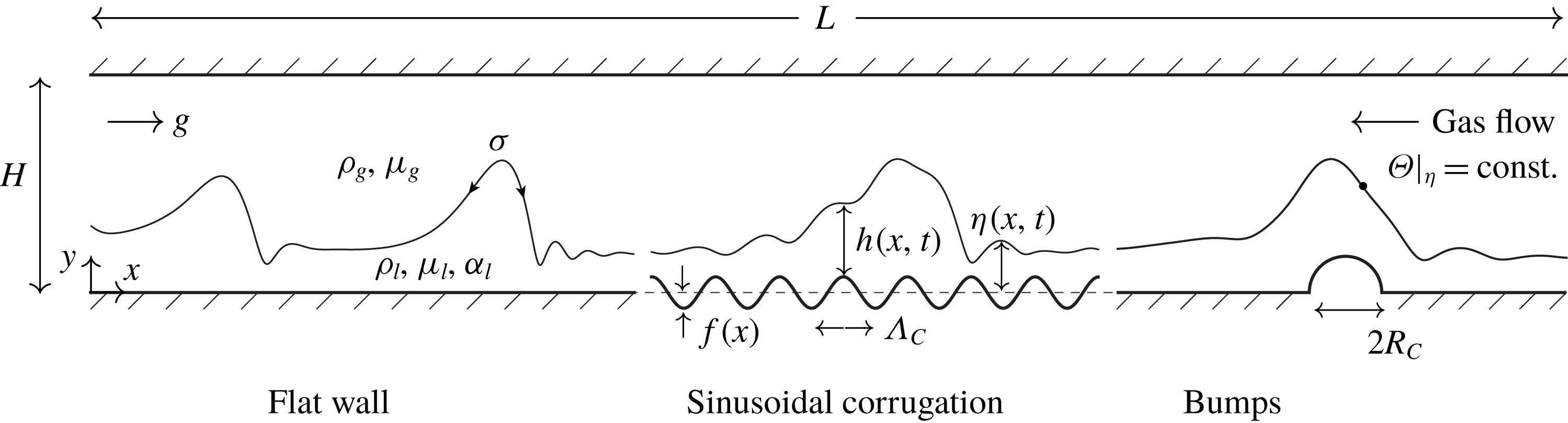
Set-up of our numerical simulations: liquid film falling down a vertical corrugated wall in contact with a strongly confined counter-current gas flow in the presence of interfacial scalar transfer. All lengths have been non-dimensionalised with the thickness
 $h_{Nu}$
of a fully developed waveless film falling on a flat surface (Nusselt Reference Nusselt1923). Three types of wall geometries are considered: (i) flat wall; (ii) sinusoidal corrugation of wavelength
 $\unicode[STIX]{x1D6EC}_{C}$
and amplitude
 ${\hat{h}}_{C}$
; (iii) semicircular bumps of radius
 $R_{C}$
and separation
 $\unicode[STIX]{x1D6EC}_{C}$
. The corrugated surface
 $y=f(x)$
follows the profile function
 $f(x)$
defined in (4.1). Parameter values are specified in § 4. The symbol
 $\unicode[STIX]{x1D6E9}$
represents the transported scalar (temperature or mass fraction) and
 $\unicode[STIX]{x1D6FC}_{l}$
the associated diffusivity.

Our study aims to answer these questions based on direct numerical simulations of the model problem represented in figure 1. It consists of a wavy liquid film falling along a vertical corrugated wall in interaction with a counter-current gas flow confined by a second flat wall. In particular, we investigate to what extent different types of wall corrugations intensify interfacial scalar transfer by acting on the surface waves, and we confront periodic and noise-driven wave regimes. As we focus on strongly confined geometries, we also assess the effect of corrugations on the gas pressure drop and whether they can trigger the flooding of the channel when the gas velocity is increased.
We consider three types of wall geometries: (i) a flat wall for reference; (ii) a sinusoidal corrugation with parameters close to those found in real structured packings (Trifonov Reference Trifonov2007a ); and (iii) a heuristic design consisting of isolated semicircular bumps (Veremieiev, Thompson & Gaskell Reference Veremieiev, Thompson and Gaskell2015) distanced roughly by the characteristic wavelength of large-amplitude surface waves. Our simulations are two-dimensional and thus represent corrugations that impose height variations only in the streamwise direction.
We restrict our study to liquid-controlled transfer by effectively imposing a fixed value for the transported scalar
 $\unicode[STIX]{x1D6E9}$
(temperature or mass fraction) at the film surface, in accordance with Albert, Marschall & Bothe (Reference Albert, Marschall and Bothe2013). In this case, heat and mass transfer are fully analogous and we treat them as one, referring simply to scalar transfer throughout the manuscript. Further, by considering moderate versus large values of the Péclet number
 $Pe={\mathcal{U}}{\mathcal{L}}/\unicode[STIX]{x1D6FC}_{l}$
, we distinguish transport regimes that are representative of heat versus mass transport (
 $\unicode[STIX]{x1D6FC}_{l}$
designates the diffusivity of the transported scalar in the liquid, and
 ${\mathcal{U}}$
and
 ${\mathcal{L}}$
are the velocity and length scales, which will be introduced in § 3).
Our simulations were performed with the finite-volume solver Gerris (Popinet Reference Popinet2009), which has been validated for the simulation of falling films on flat substrates (Dietze Reference Dietze2016). In several aspects, they are similar to those of Albert et al. (Reference Albert, Marschall and Bothe2013), who studied interfacial transfer in liquid films falling down flat walls. We extend their work by focussing on corrugated substrates and by taking into account a strongly confined counter-current gas flow.
Three previous works in particular have studied scalar transfer in liquid films falling down corrugated substrates. Haroun, Legendre & Raynal (Reference Haroun, Legendre and Raynal2010) numerically simulated a liquid film falling on a large-scale corrugation and showed that interfacial mass transfer is accurately predicted by penetration theory (Higbie Reference Higbie1935) based on the fluid velocity at the film surface. In contrast to our study, their falling film did not exhibit surface waves, which are known to significantly modify transport within the liquid (the authors did study surface waves on a flat substrate in the accompanying thesis of Haroun (Reference Haroun2008)). Kohrt et al. (Reference Kohrt, Ausner, Wozny and Repke2011) experimentally investigated the absorption of carbon dioxide by a film of silicone oil falling on a textured substrate and found the textures to increase mass transfer by up to 80 per cent. Also, the presence of a counter-current gas flow was shown to further intensify transfer even though the absorption was liquid-side controlled. In contrast to our study, the authors focused on an integral characterisation of the system and did not provide information about the existence and role of surface waves.
Gaskell et al. (Reference Gaskell, Jimack, Sellier and Thompson2006) simulated a falling film flowing over isolated hemispherical or semi-cylindrical bumps and studied the evaporation of a volatile component dissolved in the liquid. They came to the conclusion that only the three-dimensional corrugations significantly modify the concentration within the film. However, their evaporation model assumed a fully mixed liquid phase, which corresponds to the limit of small Péclet number
 $Pe$
. By contrast, our study focuses on moderate to large values of
 $Pe$
, where we have found two-dimensional isolated bumps to significantly modify scalar transport in the film as a result of hydrodynamical mixing.
For a liquid film flowing down a flat surface, the dynamics of the surface waves, which result from the well-known Kapitza instability (Kapitza Reference Kapitza1948), as well as the waves’ positive effect on scalar transfer have been widely studied (Alekseenko et al. Reference Alekseenko, Nakoryakov and Pokusaev1994; Miyara Reference Miyara1999; Adomeit, Leefken & Renz Reference Adomeit, Leefken, Renz, Hahne, Heidemann and Spindler2000; Chang & Demekhin Reference Chang and Demekhin2002; Malamataris, Vlachogiannis & Bontozoglou Reference Malamataris, Vlachogiannis and Bontozoglou2002; Serifi & Bontozoglou Reference Serifi and Bontozoglou2004; Kunugi & Kino Reference Kunugi and Kino2005; Schagen & Modigell Reference Schagen and Modigell2005; Kalliadasis et al. Reference Kalliadasis, Ruyer-Quil, Scheid and Velarde2012; Albert et al. Reference Albert, Marschall and Bothe2013; Markides, Mathie & Charogiannis Reference Markides, Mathie and Charogiannis2016). We discuss only those findings most relevant for our current work.
Yoshimura, Nosoko & Nagata (Reference Yoshimura, Nosoko and Nagata1996) experimentally investigated oxygen absorption by a vertically falling wavy water film and reported an up to twofold increase of the global interfacial transfer coefficient when surface waves were excited through a periodic inlet perturbation. Maximal intensification was observed for low-frequency large-amplitude solitary waves (see also Rastaturin, Demekhin & Kalaidin (Reference Rastaturin, Demekhin and Kalaidin2006)), which are known to contain a moving-frame vortex viewed in the wave-fixed reference frame (Brauner Reference Brauner1987; Miyara Reference Miyara1999; Alekseenko et al. Reference Alekseenko, Antipin, Bobylev and Markovich2007). This vortex is bounded by two interfacial stagnation points, one in the wave front, where enriched liquid is sucked from the film surface, and one at the back of the wave, where fresh liquid from the bulk is pushed onto the film surface (Bontozoglou Reference Bontozoglou1998). Direct numerical simulations clearly show this mechanism at work (Nagasaki & Hijikata Reference Nagasaki and Hijikata1990; Islam, Miyara & Setoguchi Reference Islam, Miyara and Setoguchi2009). The upper stagnation point represents a renewal point for the scalar free-surface layer developing into the upstream residual film. By this, we mean the thin diffusion layer of the transported scalar forming at the film surface, analogous to a boundary layer forming on a rigid wall. As a result, the free-surface layer in between successive solitary wave humps is thin and this increases overall scalar transfer.
However, the mechanism is most effective only in the early stages and subsides once the liquid pushed toward the upstream stagnation point of the moving-frame vortex is no longer fresh (Roberts & Chang Reference Roberts and Chang2000). In our current study, we have found that this decay can be effectively counteracted by intermittently disrupting the vortex through the bump-shaped wall corrugations in figure 1.
The hydrodynamics of falling liquids films flowing down corrugated substrates has also received a lot of attention (Trifonov Reference Trifonov1998; Vlachogiannis & Bontozoglou Reference Vlachogiannis and Bontozoglou2002; Wierschem, Scholle & Aksel Reference Wierschem, Scholle and Aksel2003; Dávalos-Orozco Reference Dávalos-Orozco2007; Trifonov Reference Trifonov2007b ; Oron & Heining Reference Oron and Heining2008; Pollak & Aksel Reference Pollak and Aksel2013; Tseluiko, Blyth & Papageorgiou Reference Tseluiko, Blyth and Papageorgiou2013; Trifonov Reference Trifonov2014; Schörner, Reck & Aksel Reference Schörner, Reck and Aksel2016; Trifonov Reference Trifonov2017; Schörner & Aksel Reference Schörner and Aksel2018; Schörner et al. Reference Schörner, Reck, Aksel and Trifonov2018). Aksel & Schörner (Reference Aksel and Schörner2018) have recently published an extensive review of these works. Again, we discuss only those findings most relevant for our current study. Bontozoglou & Papapolymerou (Reference Bontozoglou and Papapolymerou1997, Reference Bontozoglou and Papapolymerou1998) and Heining et al. (Reference Heining, Bontozoglou, Aksel and Wierschem2009) found states of resonance of the steady base flow, where the deflection of the film surface strongly exhibits the imprint of the corrugations. Trifonov (Reference Trifonov2007a ) and Cao, Vlachogiannis & Bontozoglou (Reference Cao, Vlachogiannis and Bontozoglou2013) demonstrated that large-amplitude solitary waves travelling over short corrugations become significantly modulated by short-wave oscillations above a threshold Reynolds number. Trifonov (Reference Trifonov2011) demonstrated that these modulations produce intricate flow structures within the wavy liquid film. This has prompted us to investigate whether such flow structures noticeably affect interfacial scalar transfer.
Cao et al. (Reference Cao, Vlachogiannis and Bontozoglou2013) found that wall corrugations may select certain surface waves from a noise-sustained wave regime. At the same time, Rastaturin et al. (Reference Rastaturin, Demekhin and Kalaidin2006) have shown, for films flowing over flat substrates, that optimally excited periodic waves intensify scalar transfer to a greater extent than naturally evolving waves. This has prompted us to investigate whether wall corrugations can indirectly benefit/deteriorate scalar transfer through wave selection.
The falling film in figure 1 is in interaction with a counter-current gas flow, which can cause an amplification of surface waves up to the point of flooding the channel (Vlachos et al. Reference Vlachos, Paras, Mouza and Karabelas2001). For weakly confined liquid films falling on flat (Trifonov Reference Trifonov2010a ,Reference Trifonov b ; Tseluiko & Kalliadasis Reference Tseluiko and Kalliadasis2011) or corrugated (Trifonov Reference Trifonov2011) substrates, it has been concluded that surface waves are significantly affected only under turbulent gas flow conditions. For strongly confined films, Dietze & Ruyer-Quil (Reference Dietze and Ruyer-Quil2013) observed flooding also under laminar gas flow conditions as a result of wave coalescence in a noise-sustained wave regime. This has prompted us to investigate whether the bump-shaped corrugations in figure 1 can trigger flooding events when the gas velocity is increased.
Our manuscript is structured as follows. Section 2 introduces the governing equations and boundary conditions and § 3 details the employed numerical method. Corrugation geometries and flow conditions are quantified in § 4. Section 5 presents the results of our simulations for forced (§ 5.1) and noise-driven (§ 5.2) surface waves, by comparing moderate and large Péclet number regimes and different wall corrugations. In § 5.3, we assess the effect of wall corrugations on the gas pressure drop and, for the bump-shaped corrugations, whether they can trigger flooding events. Conclusions are drawn in § 6. Appendices A and B, concern the validation of the numerical method employed.
2 Governing equations
We consider the configuration in figure 1, assuming constant-property Newtonian fluids for the liquid film (index ‘
 $l$
’) and counter-current gas (index ‘
 $g$
’) as well as laminar flow conditions. The flow is governed by the two-dimensional continuity and Navier–Stokes equations in the liquid (
 $k=l$
) and gas (
 $k=g$
), which are written here in dimensionless form, introducing the Kronecker symbol
 $\unicode[STIX]{x1D6FF}_{ij}$
and using Einstein’s notation (
 $i,j=1,2$
corresponding to coordinates
 $x$
,
 $y$
and velocity components
 $u_{1}=u$
,
 $u_{2}=v$
):
 $$\begin{eqnarray}\displaystyle \left.\begin{array}{@{}c@{}}\displaystyle \unicode[STIX]{x2202}_{t}u_{i}+u_{j}\unicode[STIX]{x2202}_{x_{j}}u_{i}=-\unicode[STIX]{x2202}_{x_{i}}p+\frac{X_{k}}{Re}\unicode[STIX]{x2202}_{x_{j}x_{j}}u_{i}+\frac{\unicode[STIX]{x1D6FF}_{i1}}{Fr^{2}},\quad \unicode[STIX]{x2202}_{x_{j}}u_{j}=0,\\ \displaystyle X_{l}=1,\quad X_{g}=\frac{\unicode[STIX]{x1D6F1}_{\unicode[STIX]{x1D707}}}{\unicode[STIX]{x1D6F1}_{\unicode[STIX]{x1D70C}}},\quad Re=\frac{\unicode[STIX]{x1D70C}_{l}{\mathcal{U}}{\mathcal{L}}}{\unicode[STIX]{x1D707}_{l}}=\frac{q_{Nu}}{\unicode[STIX]{x1D708}_{l}},\quad Fr=\frac{{\mathcal{U}}}{g^{1/2}{\mathcal{L}}^{1/2}}=\left[\frac{Re}{3}\right]^{1/2}.\end{array}\right\} & & \displaystyle\end{eqnarray}$$
For non-dimensionalisation, we have used the scales of the so-called Nusselt film (Nusselt Reference Nusselt1923), a fully developed waveless film falling along a flat wall in a passive atmosphere. The length scale
 ${\mathcal{L}}=h_{Nu}$
corresponds to the thickness of the Nusselt film and is related to the dimensional flow rate per unit width
 $q_{Nu}$
through
 $h_{Nu}=(3q_{Nu}\unicode[STIX]{x1D708}_{l}/g)^{1/3}$
, where
 $\unicode[STIX]{x1D708}_{l}$
is the kinematic viscosity of the liquid and
 $g$
designates the gravitational acceleration. The velocity scale corresponds to the mean velocity of the Nusselt film
 ${\mathcal{U}}=q_{Nu}/h_{Nu}$
and the time scale
 ${\mathcal{T}}={\mathcal{L}}/{\mathcal{U}}$
. The pressure
 $p$
is non-dimensionalised with
 $\unicode[STIX]{x1D70C}_{k}{\mathcal{U}}^{2}$
. The resulting dimensionless groups are the Reynolds and Froude numbers
 $Re$
and
 $Fr$
, and the density and viscosity ratios
 $\unicode[STIX]{x1D6F1}_{\unicode[STIX]{x1D70C}}=\unicode[STIX]{x1D70C}_{g}/\unicode[STIX]{x1D70C}_{l}$
and
 $\unicode[STIX]{x1D6F1}_{\unicode[STIX]{x1D707}}=\unicode[STIX]{x1D707}_{g}/\unicode[STIX]{x1D707}_{l}$
. Due to our scaling,
 $Fr$
is a function of
 $Re$
and is retained only to highlight explicitly where gravity intervenes in (2.1).
At the free surface
 $y=\unicode[STIX]{x1D702}(x,t)$
, continuity of velocity and normal/tangential stress balances yield four interfacial coupling conditions in addition to the so-called kinematic condition (relating free-surface velocity and surface position
 $\unicode[STIX]{x1D702}$
)
 $$\begin{eqnarray}\displaystyle \left.\begin{array}{@{}c@{}}\displaystyle u_{l}=u_{g},\quad v_{l}=v_{g}=\unicode[STIX]{x2202}_{t}\unicode[STIX]{x1D702}+u_{l}\unicode[STIX]{x2202}_{x}\unicode[STIX]{x1D702},\\ \displaystyle p_{l}+\frac{1}{Re}[\unicode[STIX]{x1D61A}_{ij}^{l}\boldsymbol{\cdot }n_{j}]\boldsymbol{\cdot }n_{i}=\unicode[STIX]{x1D6F1}_{\unicode[STIX]{x1D70C}}p_{g}+\frac{\unicode[STIX]{x1D6F1}_{\unicode[STIX]{x1D707}}}{Re}[\unicode[STIX]{x1D61A}_{ij}^{g}\boldsymbol{\cdot }n_{j}]\boldsymbol{\cdot }n_{i}+We\unicode[STIX]{x1D705},\\ \displaystyle [\unicode[STIX]{x1D61A}_{ij}^{l}\boldsymbol{\cdot }n_{j}]\boldsymbol{\cdot }\unicode[STIX]{x1D70F}_{i}=\unicode[STIX]{x1D6F1}_{\unicode[STIX]{x1D707}}[\unicode[STIX]{x1D61A}_{ij}^{g}\boldsymbol{\cdot }n_{j}]\boldsymbol{\cdot }\unicode[STIX]{x1D70F}_{i},\end{array}\right\} & & \displaystyle\end{eqnarray}$$
where the orthonormal surface coordinate system (
 $\boldsymbol{n}$
,
 $\unicode[STIX]{x1D749}$
) was introduced:
 $$\begin{eqnarray}\displaystyle \boldsymbol{n}=[-\unicode[STIX]{x2202}_{x}\unicode[STIX]{x1D702},1](1+\unicode[STIX]{x2202}_{x}^{2}\unicode[STIX]{x1D702})^{-1/2},\quad \unicode[STIX]{x1D749}=[1,\unicode[STIX]{x2202}_{x}\unicode[STIX]{x1D702}](1+\unicode[STIX]{x2202}_{x}^{2}\unicode[STIX]{x1D702})^{-1/2}, & & \displaystyle\end{eqnarray}$$
and where
 $\unicode[STIX]{x1D61A}_{ij}^{k}$
designates the dimensionless strain rate tensor in the liquid and gas
 $$\begin{eqnarray}\displaystyle S_{ij}^{k}={\textstyle \frac{1}{2}}(\unicode[STIX]{x2202}_{x_{j}}u_{i}+\unicode[STIX]{x2202}_{x_{i}}u_{j}). & & \displaystyle\end{eqnarray}$$
The Weber number
 $We$
(containing the surface tension
 $\unicode[STIX]{x1D70E}$
) and the dimensionless curvature of the free surface
 $\unicode[STIX]{x1D705}$
are defined as:
 $$\begin{eqnarray}\displaystyle We=\frac{\unicode[STIX]{x1D70E}}{\unicode[STIX]{x1D70C}_{l}{\mathcal{L}}{\mathcal{U}}^{2}},\quad \unicode[STIX]{x1D705}=-\unicode[STIX]{x1D735}\boldsymbol{\cdot }\boldsymbol{n}. & & \displaystyle\end{eqnarray}$$
Following Albert et al. (Reference Albert, Marschall and Bothe2013), we consider liquid-controlled interfacial scalar transfer and assume an ideally mixed gas phase. The transfer problem then reduces to solving the liquid-side convection–diffusion equation
 $$\begin{eqnarray}\displaystyle \unicode[STIX]{x2202}_{t}\unicode[STIX]{x1D6E9}+u_{j}\unicode[STIX]{x2202}_{x_{j}}\unicode[STIX]{x1D6E9}=\frac{1}{Pe}\unicode[STIX]{x2202}_{x_{j}x_{j}}\unicode[STIX]{x1D6E9}, & & \displaystyle\end{eqnarray}$$
subject to a Dirichlet condition at the film surface
 $$\begin{eqnarray}\displaystyle \unicode[STIX]{x1D6E9}|_{\unicode[STIX]{x1D702}}=1. & & \displaystyle\end{eqnarray}$$
We have written (2.6) and (2.7) in terms of the normalised liquid-side scalar
 $\unicode[STIX]{x1D6E9}=(\unicode[STIX]{x1D717}_{l}-\unicode[STIX]{x1D717}_{l}^{0})/(\unicode[STIX]{x1D717}_{l}|_{\unicode[STIX]{x1D702}}-\unicode[STIX]{x1D717}_{l}^{0})$
, where
 $\unicode[STIX]{x1D717}_{l}^{0}$
and
 $\unicode[STIX]{x1D717}_{l}|_{\unicode[STIX]{x1D702}}$
denote the values of the liquid-side scalar
 $\unicode[STIX]{x1D717}_{l}$
at the liquid inlet and film surface, which are both fixed. Furthermore,
 $Pe={\mathcal{U}}{\mathcal{L}}/\unicode[STIX]{x1D6FC}_{l}$
designates the Péclet number and
 $\unicode[STIX]{x1D6FC}_{l}$
the diffusivity of the scalar in the liquid.
We assume no slip and no penetration at the bounding walls and an adiabatic condition for the scalar at the corrugated wall
 $$\begin{eqnarray}\displaystyle u|_{y=f(x)}=v|_{y=f(x)}=u|_{y=H}=v|_{y=H}=0,\quad (\unicode[STIX]{x2202}_{y}-\unicode[STIX]{x2202}_{x}f\unicode[STIX]{x2202}_{x})\unicode[STIX]{x1D6E9}|_{y=f(x)}=0, & & \displaystyle\end{eqnarray}$$
where
 $f(x)$
represents the profile of the corrugation (see (4.1) in § 4). At
 $x=0$
, we impose a constant film thickness
 $h|_{x=0}=1$
and parabolic streamwise velocity profiles in the liquid and gas
 $$\begin{eqnarray}\displaystyle \left.\begin{array}{@{}c@{}}\displaystyle u_{l}|_{x=0}=[1+F(t)]6(\unicode[STIX]{x1D709}-\unicode[STIX]{x1D709}^{2}),\quad \unicode[STIX]{x1D709}=y-f|_{x=0},\\ \displaystyle u_{g}|_{x=0}=\frac{q_{g}}{H-\unicode[STIX]{x1D702}_{0}}6(\unicode[STIX]{x1D709}-\unicode[STIX]{x1D709}^{2}),\quad \unicode[STIX]{x1D709}=\frac{y-\unicode[STIX]{x1D702}_{0}}{H-\unicode[STIX]{x1D702}_{0}},\end{array}\right\} & & \displaystyle\end{eqnarray}$$
where
 $0\leqslant \unicode[STIX]{x1D709}\leqslant 1$
denotes the relative position within the liquid and gas layers,
 $\unicode[STIX]{x1D702}_{0}=h|_{x=0}+f|_{x=0}$
is the film surface position at the liquid inlet and
 $q_{g}$
designates the (dimensionless) gas flow rate. The liquid flow is perturbed in time through the function
 $F(t)$
, which is used to excite waves on the film surface (see (4.2) in § 4). By contrast, the gas flow remains at a constant counter-current flow rate
 $q_{g}<0$
. Further,
 $v|_{x=0}=0$
and
 $\unicode[STIX]{x2202}_{x}p|_{x=0}=0$
in both phases and also
 $\unicode[STIX]{x1D6E9}|_{x=0}=0$
.
At the end of the computational domain,
 $x=L$
, homogeneous Neumann conditions are imposed for the velocities and the scalar
 $$\begin{eqnarray}\displaystyle \unicode[STIX]{x2202}_{x}u_{k}|_{x=L}=\unicode[STIX]{x2202}_{x}v_{k}|_{x=L}=\unicode[STIX]{x2202}_{x}\unicode[STIX]{x1D6E9}|_{x=L}=0, & & \displaystyle\end{eqnarray}$$
whereas the pressure there is fixed by the Dirichlet condition
 $p|_{x=L}=0$
. However, whenever flow reversal occurs within the liquid film at the domain outlet
 $x=L$
, i.e. whenever one of the separation eddies forming underneath the troughs of the precursory capillary ripples (Dietze, Leefken & Kneer Reference Dietze, Leefken and Kneer2008; Malamataris & Balakotaiah Reference Malamataris and Balakotaiah2008) is leaving the domain, the pressure in the liquid is set to
 $p|_{x=L}=-(1/2)(u|_{x=L}^{2}+v|_{x=L}^{2})$
(Dietze & Ruyer-Quil Reference Dietze and Ruyer-Quil2013). In other words, during these short time intervals, the value of
 $p|_{x=L}$
in the liquid is reduced below its usual value
 $p|_{x=L}=0$
by an increment corresponding to the local instantaneous dynamic pressure (whereas the gas pressure remains unchanged). This ensures that the flow reversal zones are advected out of the domain. Otherwise, they would be blocked at the domain outlet and continuingly suck liquid into the domain.
As initial conditions, we impose a flat-film surface
 $\unicode[STIX]{x1D702}|_{t=0}=1$
, a semi-parabolic streamwise velocity profile in the liquid
 $u_{l}|_{t=0}=3(\unicode[STIX]{x1D709}-\unicode[STIX]{x1D709}^{2}/2)$
, with
 $\unicode[STIX]{x1D709}=y/h|_{t=0}$
, a parabolic streamwise velocity profile in the gas
 $u_{g}|_{t=0}=q_{g}/(H-\unicode[STIX]{x1D702}_{0})6(\unicode[STIX]{x1D709}-\unicode[STIX]{x1D709}^{2})$
, with
 $\unicode[STIX]{x1D709}=(y-\unicode[STIX]{x1D702}_{0})/(H-\unicode[STIX]{x1D702}_{0})$
, and, for the normalised liquid-side scalar, we impose
 $\unicode[STIX]{x1D6E9}|_{t=0}=0$
. Surface waves resulting from the initial conditions exhibit an unnaturally large amplitude and thus one needs to wait until they have been flushed out of the domain. To avoid flooding during this start-up process, the gas flow rate
 $q_{g}$
was reduced to 10 per cent of its nominal final value until the first surface wave caused by the inlet perturbation had reached the domain outlet.
3 Numerical method
Our direct numerical simulations were performed with the finite volume solver Gerris (Popinet Reference Popinet2009), which is based on the volume of fluid (VOF) (Hirt & Nichols Reference Hirt and Nichols1981) and continuum surface force (CSF) (Brackbill, Kothe & Zemach Reference Brackbill, Kothe and Zemach1992) methods. The code solves the Navier–Stokes equations for a single fluid on the entire computational domain (figure 1), along with a purely convective equation for the liquid volume fraction
 $\unicode[STIX]{x1D719}$
, while enforcing a divergence-free velocity field
 $\unicode[STIX]{x2202}_{\tilde{x}_{j}}\tilde{u} _{j}=0$
:
 $$\begin{eqnarray}\displaystyle & \displaystyle \bar{\unicode[STIX]{x1D70C}}\unicode[STIX]{x2202}_{\tilde{t}}\tilde{u} _{i}+\bar{\unicode[STIX]{x1D70C}}\tilde{u} _{j}\unicode[STIX]{x2202}_{\tilde{x}_{j}}\tilde{u} _{i}=-\unicode[STIX]{x2202}_{\tilde{x}_{i}}\tilde{p}+\bar{\unicode[STIX]{x1D70C}}g_{i}+\bar{\unicode[STIX]{x1D707}}\unicode[STIX]{x2202}_{\tilde{x}_{j}\tilde{x}_{j}}\tilde{u} _{i}+F_{\unicode[STIX]{x1D70E}i}^{\prime \prime \prime }, & \displaystyle\end{eqnarray}$$
 $$\begin{eqnarray}\displaystyle & \displaystyle \unicode[STIX]{x2202}_{\tilde{t}}\unicode[STIX]{x1D719}+\tilde{u} _{i}\unicode[STIX]{x2202}_{\tilde{x}_{i}}\unicode[STIX]{x1D719}=0. & \displaystyle\end{eqnarray}$$
 $\unicode[STIX]{x1D719}$
:
 $$\begin{eqnarray}\displaystyle \bar{\unicode[STIX]{x1D70C}}=\unicode[STIX]{x1D719}\unicode[STIX]{x1D70C}_{l}+(1-\unicode[STIX]{x1D719})\unicode[STIX]{x1D70C}_{g},\quad \bar{\unicode[STIX]{x1D707}}=\unicode[STIX]{x1D719}\unicode[STIX]{x1D707}_{l}+(1-\unicode[STIX]{x1D719})\unicode[STIX]{x1D707}_{g}. & & \displaystyle\end{eqnarray}$$
Equation (3.1b
) is discretised based on a piecewise linear reconstruction of the interface (Youngs Reference Youngs1982). The source term
 $F_{\unicode[STIX]{x1D70E}i}^{\prime \prime \prime }$
in (3.1a
) accounts for the contribution of capillary forces in the normal coupling condition (2.2)
 $$\begin{eqnarray}\displaystyle F_{\unicode[STIX]{x1D70E}i}^{\prime \prime \prime }=\unicode[STIX]{x1D6FF}_{s}\unicode[STIX]{x1D70E}\hat{\tilde{\unicode[STIX]{x1D705}}}\hat{n}_{i}, & & \displaystyle\end{eqnarray}$$
where
 $\hat{\tilde{\unicode[STIX]{x1D705}}}$
and
 $\hat{n}_{i}$
denote numerical estimates of the interfacial curvature and normal vector, while the Dirac function
 $\unicode[STIX]{x1D6FF}_{s}$
restricts treatment to the fluid interface. Both
 $\hat{\tilde{\unicode[STIX]{x1D705}}}$
and
 $\hat{n}_{i}$
are computed based on a height function representing the interface (Rudman Reference Rudman1997), which is obtained from the volume fraction field. The corrugated wall is represented by an embedded solid boundary at which the boundary conditions are directly applied through interpolation (Calhoun Reference Calhoun1999). See appendix A, for a validation of this approach.
Scalar transfer is simulated by solving the single-fluid convection–diffusion equation
 $$\begin{eqnarray}\displaystyle \bar{\unicode[STIX]{x1D70C}}\unicode[STIX]{x2202}_{\tilde{t}}\tilde{\unicode[STIX]{x1D717}}+\bar{\unicode[STIX]{x1D70C}}\tilde{u} _{j}\unicode[STIX]{x2202}_{\tilde{x}_{j}}\tilde{\unicode[STIX]{x1D717}}=\unicode[STIX]{x2202}_{\tilde{x}_{j}}(\bar{\unicode[STIX]{x1D6FC}}\unicode[STIX]{x2202}_{\tilde{x}_{j}}\tilde{\unicode[STIX]{x1D717}}), & & \displaystyle\end{eqnarray}$$
where the transported scalar
 $\tilde{\unicode[STIX]{x1D717}}$
is defined on the entire domain. In cells containing the film surface, i.e. interfacial cells, the single-fluid diffusivity
 $\bar{\unicode[STIX]{x1D6FC}}$
is constructed by harmonic averaging
 $$\begin{eqnarray}\displaystyle \bar{\unicode[STIX]{x1D6FC}}^{-1}=\unicode[STIX]{x1D719}\unicode[STIX]{x1D6FC}_{l}^{-1}+(1-\unicode[STIX]{x1D719})\unicode[STIX]{x1D6FC}_{g}^{-1}. & & \displaystyle\end{eqnarray}$$
Such cells are identified based on the height function mentioned above, which assigns a definite position to the film surface. In all other cells,
 $\bar{\unicode[STIX]{x1D6FC}}$
is set to the respective pure-phase diffusivities
 $\unicode[STIX]{x1D6FC}_{l}$
,
 $\unicode[STIX]{x1D6FC}_{g}$
. This leads to a sharp representation of scalar transport even though the volume fraction field
 $\unicode[STIX]{x1D719}$
itself is not sharp. The choice of harmonic averaging (3.5) ensures that the diffusional resistance of interfacial cells containing both phases is physically consistent (Patankar Reference Patankar1980). For example, in the limit
 $\unicode[STIX]{x1D6FC}_{g}\rightarrow \infty$
, equation (3.5) correctly reduces to the sole liquid contribution, whereas geometric averaging would yield a diffusional resistance of zero. This limit is relevant for our simulations, where we have set
 $\unicode[STIX]{x1D6FC}_{g}>10^{3}\unicode[STIX]{x1D6FC}_{l}$
in order to implement conditions of liquid-controlled transfer (the choice of
 $\unicode[STIX]{x1D6FC}_{g}$
has no implication for the sharpness of the scalar transport representation nor for the sharpness of the film surface). Our approach allows accurate prediction of the scalar transfer through the film surface while remaining within a VOF framework. Albert et al. (Reference Albert, Marschall and Bothe2013) used a different approach by reconstructing the scalar profile near the interface with an analytical solution.
The computational domain is decomposed into a Cartesian quadtree grid, which is adaptively refined. We impose a finer grid in the liquid phase, where gradients of the transported scalar are large. In the liquid film and in the vicinity of the film surface, the (dimensionless) cell size is fixed to
 $\unicode[STIX]{x1D6E5}=H/2^{7}$
, whereas, in the gas, it is adapted based on the vorticity (
 $H/2^{2}\leqslant \unicode[STIX]{x1D6E5}\leqslant H/2^{5}$
). The grid in the vicinity of the corrugated wall is additionally refined (
 $\unicode[STIX]{x1D6E5}=H/2^{8}$
). The code employs a fractional-step projection method (Chorin Reference Chorin1968) that leads to a formally second-order accurate time discretisation (Popinet Reference Popinet2009). The time step is dynamically adapted so that
 $Co=u^{\ast }\unicode[STIX]{x1D6E5}_{t}/\unicode[STIX]{x1D6E5}_{x}\leqslant 0.8$
in each cell (
 $u^{\ast }$
denotes the magnitude of the dimensional velocity in a given cell, and
 $Co$
designates the Courant number). We have performed a grid dependence analysis, results of which are presented in appendix B.
To limit computational cost, simulations were commenced with a coarser grid until they had reached a hydrodynamically developed state. After that, the grid resolution was increased to its final level and the simulation was continued until reaching a fully developed state. This is why data in time trace plots (e.g. figures 9–11) start at a finite time
 $t>0$
.
4 Simulated cases: flow conditions and corrugations
Parameters of the numerical simulations. Lengths have been non-dimensionalised with the Nusselt film thickness, which is
 $h_{Nu}=334~\unicode[STIX]{x03BC}\text{m}$
throughout, and frequencies using the corresponding time scale
 ${\mathcal{T}}=h_{Nu}^{2}/q_{Nu}=2.61~\text{ms}$
. The liquid Reynolds number is
 $Re=15$
and the dimensionless gas flow rate
 $q_{g}=-20$
(except for case 1, where the gas is quiescent, and in § 5.3, where
 $|q_{g}|$
was increased in an additional simulation of case 5). The domain height is
 $H=4.5$
and the domain length
 $L=63H$
. For all nine cases, liquid-controlled scalar transfer was simulated for strongly dominant (
 $Pe=4590$
) and moderately dominant (
 $Pe=459$
) convection.

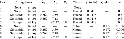
Table 1 lists the main parameters for the nine cases simulated in this study. For all simulations, the dimensionless domain height is
 $H=4.5$
and the domain length
 $L=63H$
. This corresponds to the strongly confined configuration considered in Dietze & Ruyer-Quil (Reference Dietze and Ruyer-Quil2013). Liquid properties and flow conditions are based on the experimental conditions of Dietze, Al-Sibai & Kneer (Reference Dietze, Al-Sibai and Kneer2009), for which the Gerris solver has been comprehensively validated (Dietze Reference Dietze2016). The hydrodynamical properties are the same for all cases (film of aqueous solution of dimethyl sulfoxide, DMSO, in contact with air):
 $\unicode[STIX]{x1D707}_{l}=3.13\times 10^{-3}~\text{Pa}~\text{s}$
;
 $\unicode[STIX]{x1D70C}_{l}=1098.3~\text{kg}~\text{m}^{-3}$
;
 $\unicode[STIX]{x1D70E}=0.0484~\text{N}~\text{m}^{-1}$
;
 $\unicode[STIX]{x1D707}_{g}=1.8\times 10^{-5}~\text{Pa}~\text{s}$
;
 $\unicode[STIX]{x1D70C}_{g}=1.2~\text{kg}~\text{m}^{-3}$
. The liquid Reynolds number is
 $Re=q_{Nu}\unicode[STIX]{x1D70C}_{l}/\unicode[STIX]{x1D707}_{l}=15$
and the dimensionless counter-current gas flow rate
 $q_{g}=-20$
(except for the flat-film reference simulation, case 1, where the gas is quiescent, and an additional simulation of case 5 in § 5.3, where
 $|q_{g}|$
was increased). All simulations have been performed for two different values of the Péclet number in (2.6):
 $Pe=4590$
(strongly dominant convection) and
 $Pe=459$
(moderately dominant convection).
We distinguish three types of wall corrugations, as represented in figure 1. The corrugation surface
 $y=f(x)$
is defined by the profile function
 $f(x)$
, which is given below for the flat wall (4.1a
), sinusoidal corrugation (4.1b
) and semicircular bumps (4.1c
):
 $$\begin{eqnarray}\displaystyle & \displaystyle f(x)=0, & \displaystyle\end{eqnarray}$$
 $$\begin{eqnarray}\displaystyle & \displaystyle f(x)=-{\hat{h}}_{C}\cos (2\unicode[STIX]{x03C0}x/\unicode[STIX]{x1D6EC}_{C}), & \displaystyle\end{eqnarray}$$
 $$\begin{eqnarray}\displaystyle \left.\begin{array}{@{}c@{}}f(x)=[R_{C}^{2}-(x-x_{m})^{2}]^{1/2}\quad \forall x\in [x_{m}-R_{C},x_{m}+R_{C}],\\ f(x)=0\quad \forall x\notin [x_{m}-R_{C},x_{m}+R_{C}],\quad x_{m}=k\unicode[STIX]{x1D6EC}_{C},\quad k=1,\ldots ,5.\end{array}\right\} & & \displaystyle\end{eqnarray}$$
 $\unicode[STIX]{x1D6EC}_{C}$
. In both variants,
 $\unicode[STIX]{x1D6EC}_{C}$
is smaller than the cutoff wavelength
 $\unicode[STIX]{x1D6EC}_{c}=13.2$
of the Kapitza instability for a flat-wall reference simulation (case 2). Further, the corrugation amplitude
 ${\hat{h}}$
is small so that flow separation does not occur in the corrugation troughs, in contrast to other studies (Pollak & Aksel Reference Pollak and Aksel2013; Trifonov Reference Trifonov2014; Schörner et al.
Reference Schörner, Reck and Aksel2016).
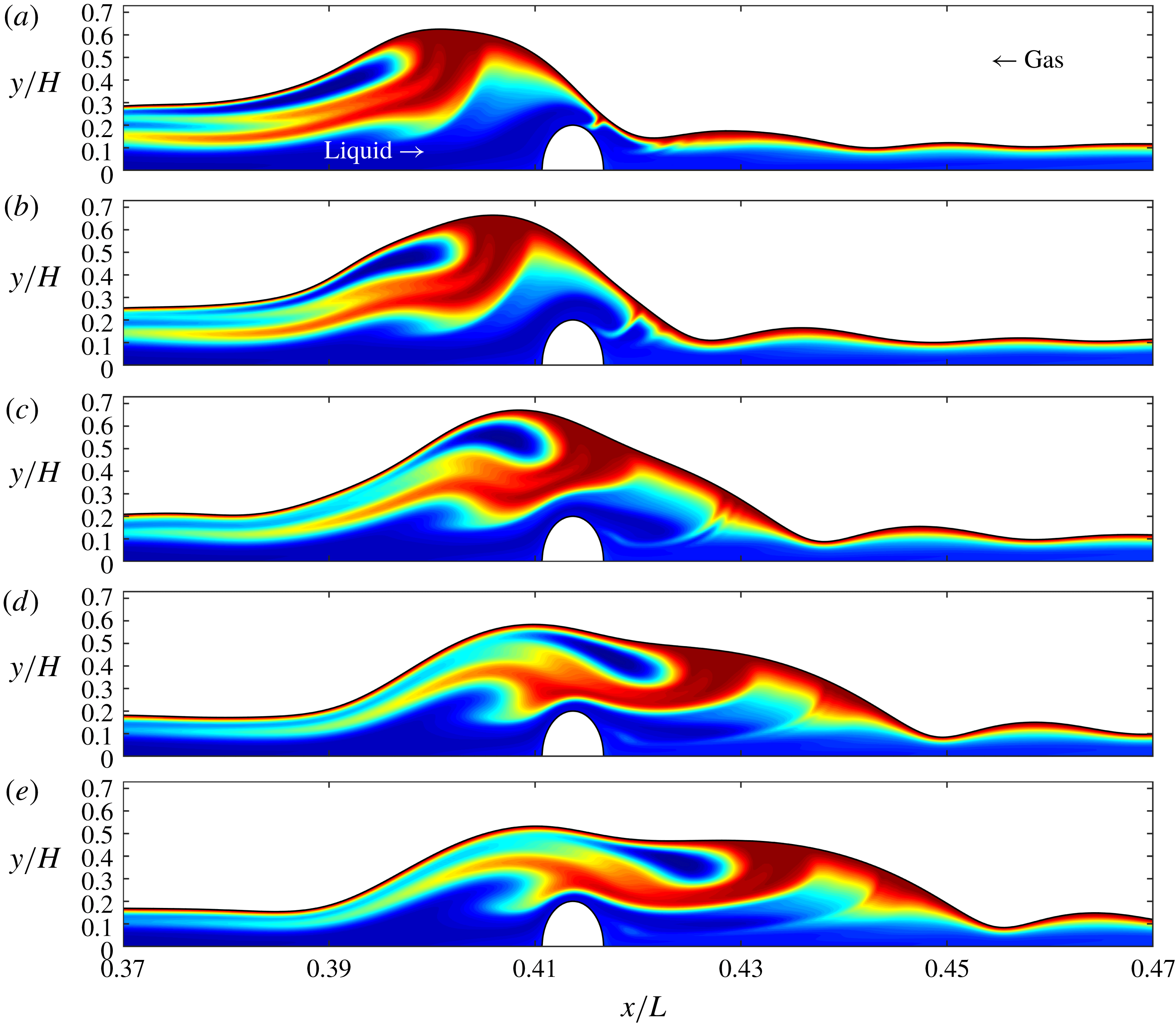
Effect of different wall-corrugations and periodically forced surface waves on scalar transport for strongly dominant convection:
 $Re=15$
,
 $f=0.0418$
,
 $Pe=4590$
. Contours highlight transported scalar
 $\unicode[STIX]{x1D6E9}$
(blue:
 $\unicode[STIX]{x1D6E9}=0$
; red:
 $\unicode[STIX]{x1D6E9}=1$
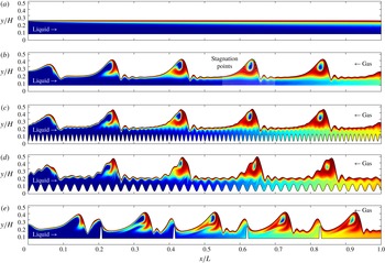
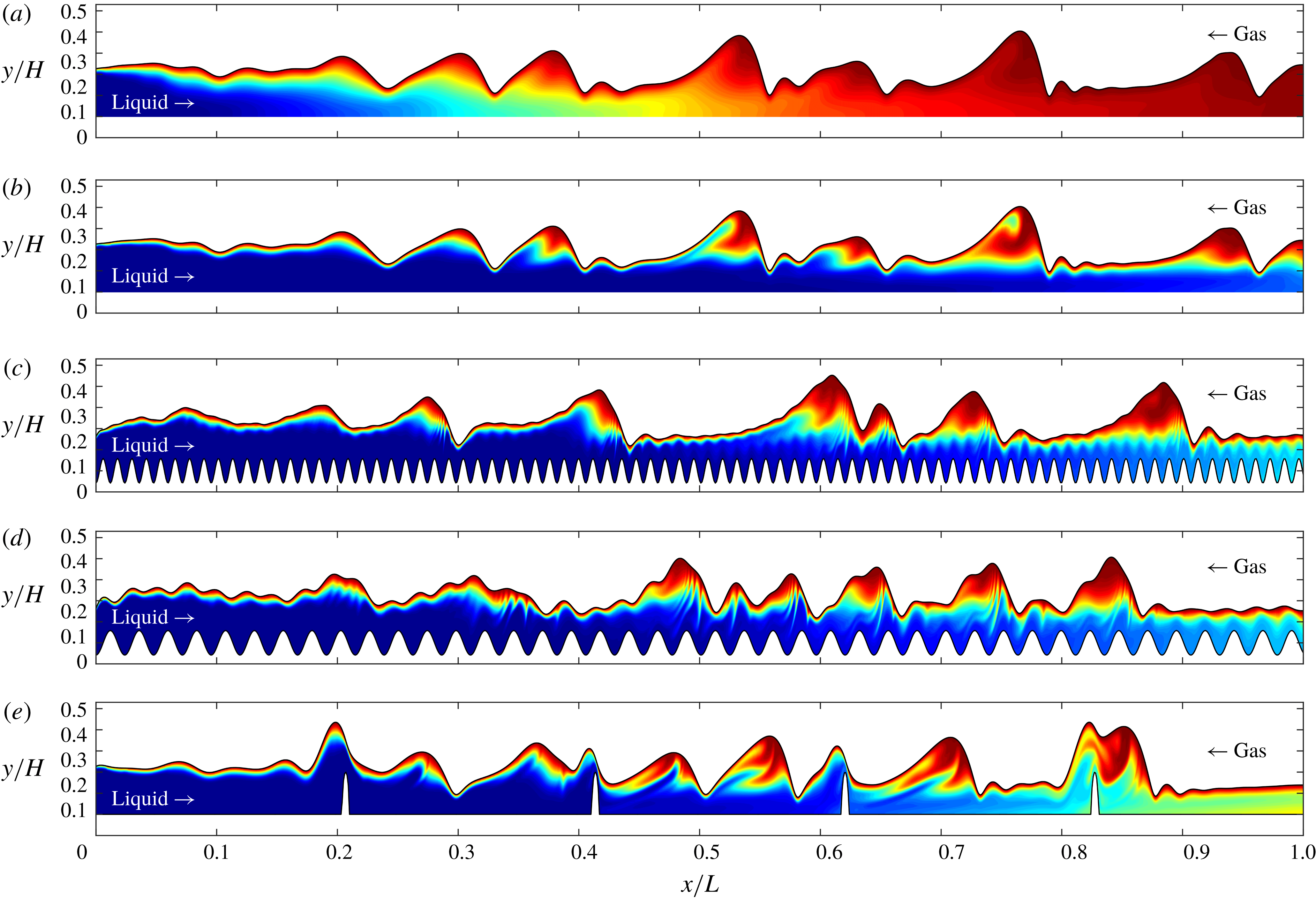
). Panels (a–e) correspond to cases 1–5 in table 1. White lines in (b) show streamlines in the moving reference frame, evidencing a vortex in the main hump.

Noise-driven surface waves (cases 6–9, table 1):
 $Re=15$
; random forcing according to (4.2b
). Contours of the transported scalar
 $\unicode[STIX]{x1D6E9}$
(blue:
 $\unicode[STIX]{x1D6E9}=0$
; red:
 $\unicode[STIX]{x1D6E9}=1$
). (a) Case 6 for moderately dominant convection
 $Pe=459$
; (b–e) cases 6, 7, 8, and 9 for strongly dominant convection
 $Pe=4590$
.

Effect of sinusoidal wall corrugations (4.1b
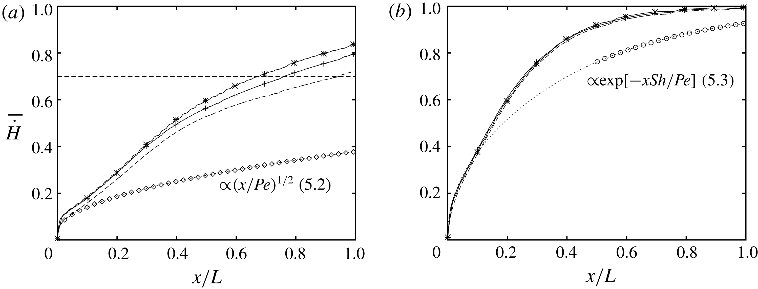
) on scalar transfer into the wavy falling film. Periodically forced surface waves (cases 2 to 4 in table 1):
 $Re=15$
,
 $f=0.0418$
. Profiles of the time-averaged convection rate
 $\bar{{\dot{H}}}$
(5.1). Dotted lines: flat-wall/flat-film reference simulation (case 1); dashed: wavy film on a flat wall (case 2); plus signs: wavy film on the short sinusoidal corrugation (
 $\unicode[STIX]{x1D6EC}_{C}=3.59$
, case 3); stars: wavy film on the long sinusoidal corrugation (
 $\unicode[STIX]{x1D6EC}_{C}=7.18$
, case 4); diamonds and circles: analytical solutions (5.2) and (5.3). (a) Strongly dominant convection:
 $Pe=4590$
. For the long sinusoidal corrugation, the transfer length required to reach the value of
 $\bar{{\dot{H}}}$
marked by the horizontal dashed line is approximately 30 % less than for the flat wall; (b) moderately dominant convection:
 $Pe=459$
.

The isolated bumps (4.1c
) are the two-dimensional analogue of the hemispherical corrugations studied in Veremieiev et al. (Reference Veremieiev, Thompson and Gaskell2015). We have simulated one such configuration (cases 5 and 9, table 1), where the distance
 $\unicode[STIX]{x1D6EC}_{C}$
between bumps was chosen to correspond roughly to the separation of large-amplitude solitary waves travelling on the film (figure 2
e), and where the radius
 $R_{C}$
is sufficiently large to disrupt these waves.
We consider two wave regimes in terms of the inlet forcing applied through the function
 $F(t)$
in (2.9). In the first case, periodic surface waves are forced by a sinusoidal monochromatic perturbation (4.2a
). In the second case, noise-driven surface waves are forced through a ‘random’ perturbation (4.2b
), which is constructed with a Fourier series (Chang, Demekhin & Kalaidin Reference Chang, Demekhin and Kalaidin1996a
). The function
 $F(t)$
for the two cases is:
 $$\begin{eqnarray}\displaystyle & \displaystyle F(t)=\unicode[STIX]{x1D716}\sin (2\unicode[STIX]{x03C0}ft), & \displaystyle\end{eqnarray}$$
 $$\begin{eqnarray}\displaystyle & \displaystyle F(t)=\unicode[STIX]{x1D716}\mathop{\sum }_{k=1}^{N}\sin (2\unicode[STIX]{x03C0}k\unicode[STIX]{x0394}ft+\unicode[STIX]{x1D711}_{rand}),\quad \unicode[STIX]{x0394}f=2f_{c}/N, & \displaystyle\end{eqnarray}$$
 $N=1000$
,
 $f$
is the frequency of the monochromatic excitation,
 $f_{c}$
designates the cutoff frequency of the Kapitza instability for the flat-wall reference case,
 $\unicode[STIX]{x1D711}_{rand}$
is a random phase shift and
 $\unicode[STIX]{x1D716}$
designates the relative inlet perturbation amplitude. Values for all parameters in (4.2) are listed in table 1. Although
 $\unicode[STIX]{x1D716}$
is much smaller for the random perturbation (cases 6–9), cumulation of the Fourier series terms in (4.2b
) yields a total amplitude for
 $F(t)$
that is comparable to that of the monochromatic forcing (cases 2–5).
An overview of our simulations is given in figures 2 and 3, showing contours of the scalar
 $\unicode[STIX]{x1D6E9}$
(blue:
 $\unicode[STIX]{x1D6E9}=0$
; red:
 $\unicode[STIX]{x1D6E9}=1$
throughout the manuscript). Figure 2 concerns simulations with periodically forced surface waves (cases 2–5, table 1) and shows the effect of different wall corrugations (figure 2
b–e) compared to the flat-wall/flat-film reference simulation (case 1, figure 2
a) for strongly dominant convection (
 $Pe=4590$
). Conversely, figure 3 shows the corrugation effect for noise-driven surface waves (cases 6–9, table 1). Figure 3(a) corresponds to moderately dominant convection (
 $Pe=459$
) and figure 3(b–e) to strongly dominant convection (
 $Pe=4590$
). The bump-shaped corrugations in figures 2(e) and 3(e) are in fact semicircular and only appear oval because the ordinate has been compressed.
5 Results and discussion
To quantify scalar transfer to the liquid film, we introduce the local instantaneous rate of convection (per unit width)
 ${\dot{H}}$
of the normalised scalar
 $\unicode[STIX]{x1D6E9}$
and its time average
 $\bar{{\dot{H}}}$
 $$\begin{eqnarray}\displaystyle {\dot{H}}(x,t)=\int _{f(x)}^{\unicode[STIX]{x1D702}(x,t)}u\unicode[STIX]{x1D6E9}\,\text{d}y,\quad \bar{{\dot{H}}}(x)=\frac{1}{t_{2}-t_{1}}\int _{t_{1}}^{t_{2}}{\dot{H}}\,\text{d}t, & & \displaystyle\end{eqnarray}$$
which expresses to what extent the film has saturated, with the transported scalar,
 $\bar{{\dot{H}}}=1$
signifying that the maximal convection rate has been reached. Further, the steeper
 $\bar{{\dot{H}}}$
increases with
 $x$
, the better the scalar is transferred to the film. We will use this quantity to characterise simulations with periodically forced surface waves (cases 2–5, table 1). In those cases, we will apply (5.1) to the temporally developed part of the simulation data, using an integration span
 $(t_{2}-t_{1})$
of two wave periods.
For the case of a hydrodynamically developed waveless film flowing on a flat wall in a passive atmosphere, analytical predictions for
 $\bar{{\dot{H}}}$
can be obtained in different limits. For strongly dominant convection (
 $Pe=4590$
in our simulations), the limit of a thin scalar free-surface layer at the film surface may be invoked (Higbie Reference Higbie1935):
 $$\begin{eqnarray}\displaystyle {\dot{H}}=\left(\frac{6}{\unicode[STIX]{x03C0}}\right)^{1/2}\left(\frac{x}{Pe}\right)^{1/2}. & & \displaystyle\end{eqnarray}$$
For moderately dominant convection (
 $Pe=459$
in our simulations), the limit of a fully developed film becomes relevant. In this case
 $$\begin{eqnarray}\displaystyle {\dot{H}}=1-\exp \left(-x\frac{Sh}{Pe}\right), & & \displaystyle\end{eqnarray}$$
where the Sherwood number
 $Sh=3.41$
(Brauer Reference Brauer1971). We will later compare (5.2) and (5.3) with our numerical simulations of case 1 (see figures 4, 6 and figure 15 in appendix B).
For the noise-driven wave regimes (cases 6–9, table 1), the computation of
 $\bar{{\dot{H}}}$
(5.1) is impractical as it requires a much longer time integration span to obtain a statistically robust spatial profile. For those cases, we will instead evaluate time traces of the total scalar content in the liquid film
 $$\begin{eqnarray}\displaystyle U_{tot}(t)=\int _{0}^{L}\int _{f(x)}^{\unicode[STIX]{x1D702}(x,t)}\unicode[STIX]{x1D6E9}\,\text{d}y\,\text{d}x. & & \displaystyle\end{eqnarray}$$
5.1 Periodically forced surface waves
We first focus on periodically forced surface waves, i.e. cases 2 to 5 in table 1, where monochromatic forcing (4.2a
) was applied with an excitation frequency
 $f=0.0418$
. This frequency produced very regular large-amplitude solitary waves in the experiments of Dietze et al. (Reference Dietze, Al-Sibai and Kneer2009), which were conducted in a vertically falling liquid film flowing down a flat wall in a quiescent unconfined atmosphere. It also roughly corresponds to the dominant frequency of the noise-driven wave spectrum on a flat wall (case 6, figure 10
b).
In §§ 5.1.1 and 5.1.2, we will investigate how different wall corrugations additionally intensify scalar transfer. Before that, we briefly recap the effect of surface waves alone, by comparing cases 1 and 2, which correspond to a falling film on a flat wall without and with surface waves. These cases are represented with the dotted and dashed lines in figure 4, showing profiles of
 $\bar{{\dot{H}}}$
(5.1) for
 $Pe=4590$
(figure 4
a) and
 $Pe=459$
(figure 4
b). Additional diamonds (
 $Pe=4590$
) and circles (
 $Pe=459$
) correspond to the analytical solutions (5.2) and (5.3), which are in good agreement with the waveless simulation (case 1, dotted lines). A detailed discussion of this comparison is provided in appendix B.
Comparing the wavy (case 2, dashed line) and waveless (case 1, dotted line) simulations in figure 4, we see that surface waves alone considerably increase scalar transfer. This is principally caused by the moving-frame vortex within the large-amplitude solitary waves (Bontozoglou Reference Bontozoglou1998; Roberts & Chang Reference Roberts and Chang2000; Islam et al. Reference Islam, Miyara and Setoguchi2009; Albert et al. Reference Albert, Marschall and Bothe2013), as was discussed in the introduction. The vortex is visualised in the wave hump of figure 2(b) by streamlines in the wave-fixed reference frame. Viewed in this frame, liquid entering the main wave hump through the capillary trough is forced to circumvent the moving-frame vortex. As a result, the free-surface layer in the wave front is destroyed, reducing transfer there, while the free-surface layer in the wave back is compressed, increasing transfer there (see Albert et al. (Reference Albert, Marschall and Bothe2013) for local transfer coefficient data). These effects are particularly visible in the second wave of figure 2(b). Thereby, the compression has a greater overall impact as it sets the inlet condition for the free-surface layer development in the long residual film separating successive wave humps.
However, this intensification mechanism weakens over time as a wave travels downstream. Indeed, the compression of the free-surface layer in the wave back only works as long as the liquid impinging on the film surface is fresh. In figure 2(b), this limit has been reached in the third wave, coinciding with a decrease in wave-induced transfer intensification, as evidenced by the reduced divergence between the dashed and dotted lines in figure 4(a) for
 $x/L\geqslant 0.4$
. We will see in the following subsections that this natural decay can be effectively countered by introducing wall corrugations.
Comparing figures 4(a) and 4(b), we see that the wave effect on scalar transfer is much stronger for
 $Pe=4590$
(figure 4
a) than for
 $Pe=459$
(figure 4
b). This is due to the increasing relative importance of convective transport with increasing
 $Pe$
.
5.1.1 Sinusoidal corrugations
For strongly dominant convection (
 $Pe=4590$
), an additional intensification of scalar transfer to the wavy liquid film can be achieved through the sinusoidal wall corrugations (4.1b
). This is evidenced by figure 4(a), where the
 $\bar{{\dot{H}}}$
profiles marked by stars and plus signs correspond to the short (case 3) and long (case 4) sinusoidal corrugations. We see that the transfer length
 $x/L$
required to reach a particular rate of convection
 $\bar{{\dot{H}}}=0.7$
(horizontal dashed line) is reduced by up to 30 % compared to the flat-wall reference simulation (case 2, dashed line). By contrast, no additional intensification is observed for moderately dominant convection (
 $Pe=459$
, figure 4
b).
The wall corrugations affect the free-surface layer development in two ways. Firstly, they generate small-amplitude surface ripples of corresponding wavelength on the residual film separating large humps (Bontozoglou & Papapolymerou Reference Bontozoglou and Papapolymerou1997, Reference Bontozoglou and Papapolymerou1998; Heining et al. Reference Heining, Bontozoglou, Aksel and Wierschem2009). This can be seen most clearly in figure 2(d) between the second and third wave hump. The ripples do not travel and can be considered as upwellings caused as the fluid flows over the corrugation bumps. The scalar free-surface layer follows the rippled shape of the film surface and thus its transfer length is increased, leading to an increased scalar transfer rate compared to the flat-wall scenario. In principle, the effect is similar to the transfer intensification generated by small-amplitude sinusoidal surface waves travelling on falling liquid films (Rastaturin et al. Reference Rastaturin, Demekhin and Kalaidin2006). It is weaker for the short corrugation (figure 2 c) than for the long corrugation (figure 2 d) because the wall-corrugation/film-surface resonance is stronger in the latter case, leading to ripples of greater amplitude.
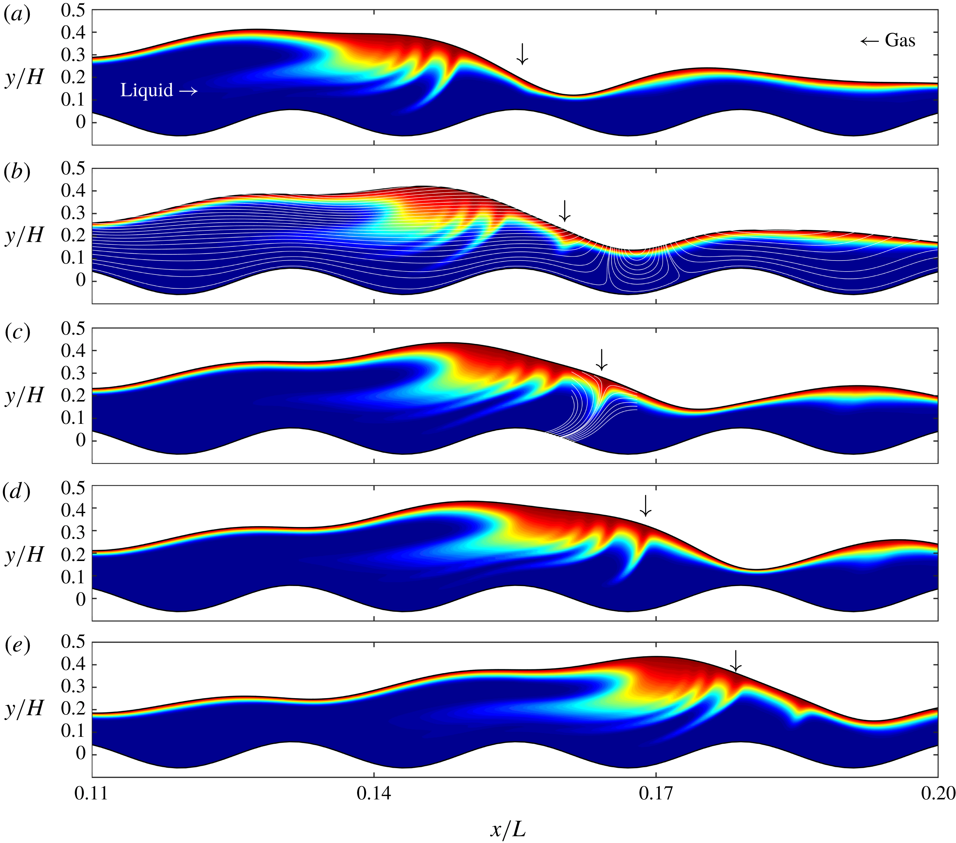
A second effect of the wall corrugations is illustrated in figure 5, where we have represented the scalar field at different times during the passage of a main wave hump over the sixth corrugation bump of the long sinusoidal corrugation (case 4). At the position marked by an arrow in the successive panels, a thin scalar plume is extruded from the scalar free-surface layer into the bulk of the film. This rapid extrusion event is repeated every time the wave front passes over the downstream flank of a corrugation bump and it represents a direct convection-induced transfer intensification mechanism. The supplementary movie 1 available online at https://doi.org/10.1017/jfm.2018.851 shows the repeated plume extrusions in action.
Repeated extrusion of plumes from the scalar free-surface layer. Long sinusoidal wall corrugation: case 4, figure 2(d). As the leading front of the main wave hump passes over the downstream flank of a corrugation bump (e.g. the sixth bump at the centre of the panels), a subduction-type flow, occurring relative to the film surface, rapidly extrudes the free-surface layer in the form of a thin plume at the position marked by the arrow. White lines in (c) represent streamlines in a frame of reference wherein the film surface around the plume is stationary (streamlines in the wall-fixed reference frame are shown in b), evidencing the subduction flow. The plume extrusions represent a direct convection-induced transfer intensification mechanism. Supplementary movie 1 shows the plume extrusions in action.

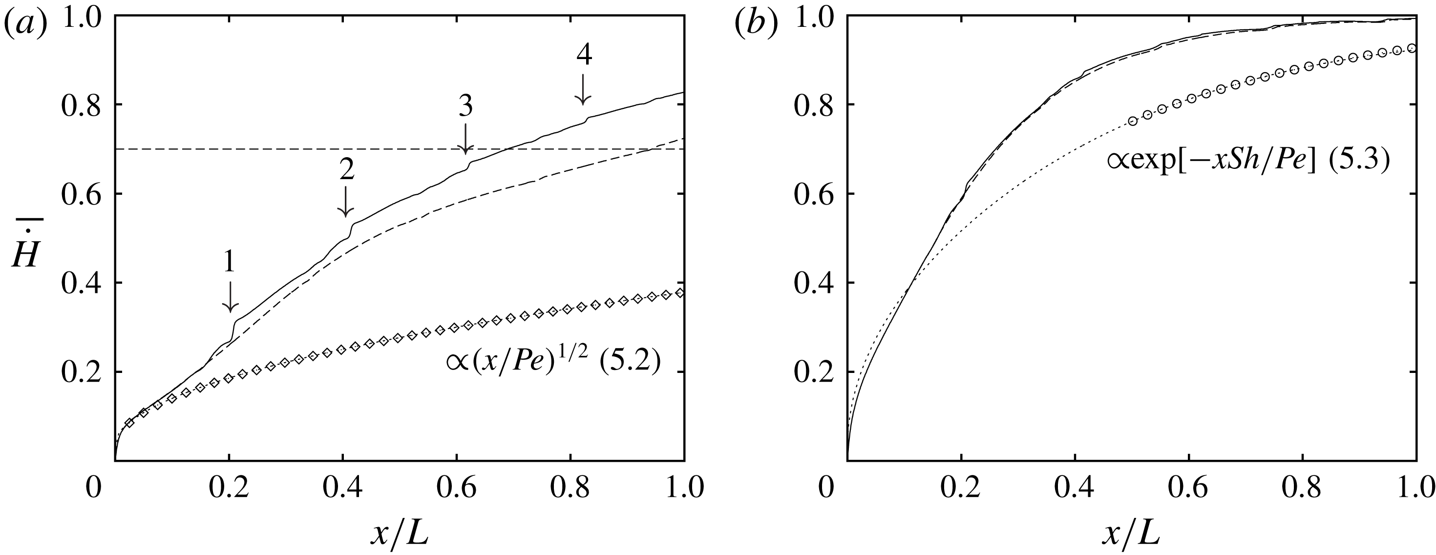
Effect of the bump-shaped wall corrugations (4.1c
) on scalar transfer into the wavy falling film. Periodically forced surface waves (cases 2 and 5, table 1):
 $Re=15$
,
 $f=0.0418$
. Profiles of the time-averaged convection rate
 $\bar{{\dot{H}}}$
(5.1). Dotted lines: flat-wall/flat-film reference simulation (case 1); dashed: wavy film on a flat wall (case 2); solid: wavy film on the bump-shaped corrugations (case 5); diamonds and circles: analytical solutions (5.2) and (5.3). (a) Strongly dominant convection:
 $Pe=4590$
. Arrows mark the position of the four corrugation bumps; (b) moderately dominant convection:
 $Pe=459$
.

The hydrodynamics of the plume extrusions becomes clear by viewing the flow in a frame of reference wherein the film surface remains stationary. In contrast to a flat wall, surface waves travelling on a sinusoidal corrugation do not attain a developed state. Instead, they are repeatedly decelerated and accelerated as they move over successive corrugation bumps and troughs. Thus, the concept of a wave-fixed reference frame is only locally applicable and such a frame must translate both in the
 $x$
- and
 $y$
-direction.
Streamlines in figure 5(c) are drawn in a reference frame moving with
 $c_{x}=1.15$
and
 $c_{y}=0.21$
. In this frame, the leading front of the main wave hump, where the scalar plume develops, remains fixed and becomes a streamline itself. The flow is then seen relative to the film surface, allowing the free-surface layer development to be understood. In particular, we observe a subduction-type flow at the location of the scalar plume, where two opposite-direction fluxes, emanating from the main hump and capillary trough, impinge on one another. As a result, the free-surface layer is entrained below the film surface, forming a plume. The plume origin coincides with an interfacial stagnation point. Upstream of this point, the fluid flows faster than the wave, and downstream, it flows slower.
For a film falling along a flat wall, interfacial stagnation points (in the wave-fixed reference frame) occur only in the main wave hump, where the film thickness is sufficiently large for the fluid velocity to surpass the wave celerity. Such stagnation points occur on either side of the moving-frame vortex in figure 2(b). By contrast, the stagnation point observed in figure 5(c) occurs in a thinner portion of the film. This follows from a local decrease in wave celerity above the downstream flank of the corrugation bumps. Indeed, the
 $x$
-translation velocity of the moving frame used in figure 5(c) (
 $c_{x}=1.15$
) is significantly smaller than the average celerity of the large wave humps (
 $c\approx 2$
), which can be determined from their spacing in figure 2(d) together with the inlet forcing frequency. The time-varying wave celerity is clearly evidenced by the supplementary movie 2, where the leading front of a wave hump is seen to periodically change steepness as it moves over the corrugation bumps and troughs.
At the same time, the fluid in the region where the scalar plume forms is strongly decelerated due to capillary pressure gradients, as evidenced by the streamlines in the wall-fixed reference frame represented in figure 5(b). These exhibit a flow reversal zone just downstream of the plume, such as typically occurs underneath the precursory capillary ripples of a falling liquid film (Dietze et al. Reference Dietze, Leefken and Kneer2008; Malamataris & Balakotaiah Reference Malamataris and Balakotaiah2008).
The active plume in figure 5 grows only as long as the leading wave front remains above the downstream flank of the sixth corrugation bump (corrugation bumps are numbered in figure 5). After that (figure 5 d,e), the subduction flow subsides and the plume is advected backward to the main hump, where it is compounded with the inactive plumes from previous extrusion events. This generates a sabretooth pattern of the scalar field within the main hump. Between figures 5(a) and 5(c), the inactive plumes increasingly approach the active one, confirming that the celerity of the wave is indeed decreased when it passes over the downstream flank of the corrugation bump.
We conclude by pointing out that the intermittent plume extrusion discussed above is akin to the findings of Albert et al. (Reference Albert, Marschall and Bothe2013), who observed oscillations of the scalar plume forming within solitary waves travelling over a flat wall. The authors attributed these oscillations to variations in wave celerity during the development of the surface waves.
5.1.2 Bump-shaped corrugations
For strongly dominant convection (
 $Pe=4590$
), the bump-shaped corrugations (4.1c
) increase scalar transfer at least as much as the sinusoidal corrugations discussed in the previous section, notwithstanding that only four of them are distributed over the entire domain (figure 2
e). This is shown in figure 6(a), where the solid line represents the convection rate
 $\bar{{\dot{H}}}$
(5.1) for the bump-shaped corrugations (case 5, table 1), whereas the dotted and dashed lines once again correspond to the flat-wall simulations without and with surface waves (cases 1 and 2). At each corrugation bump (marked by arrows in figure 6
a),
 $\bar{{\dot{H}}}$
abruptly increases with respect to the profile for the wavy film on a flat wall (case 2, dashed line). In between two bumps, the slope of the
 $\bar{{\dot{H}}}$
profile gradually reconverges toward that of the flat-wall solution, but this is interrupted time and again by the next corrugation bump. As a result, the solid and dashed profiles in figure 6(a) diverge, in particular for
 $x\geqslant 0.4$
, where the effect of the moving-frame vortex has started to decay in the flat-wall simulation (as discussed at the start of § 5.1).
The bump-shaped corrugations directly counteract this natural decay by regularly disrupting the moving-frame vortex so that the wave hump can replenish with fresh liquid, rebooting the associated intensification mechanism every time. Contours in figure 2(e) show the scalar field after such an event, evidencing a redistribution of liquid within the wave humps. In particular, a new scalar plume is seen to develop from the wave fronts. The fluid displaced by this growing plume is fresh (blue) and reinvigorates the compression of the free-surface layer in the wave back. This allows the transfer intensification mechanism caused by the moving-frame vortex to prevail.
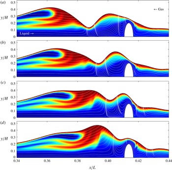
Redistribution of liquid within the main wave hump as it reaches the second corrugation bump: case 5, figure 2(e). (a–d) Correspond to times
 $t=(1.4636,1.4643,1.4651,1.4657)\times 10^{3}$
and show scalar contours and streamlines in the wall-fixed reference frame. The precursory capillary trough is lifted over the corrugation bump by the capillary-driven vortex underneath it. Upstream of the vortex, fresh (blue) liquid from the wall region is increasingly pushed upward into the wave front, causing a reconfiguration of the wave hump. Saturated (red) liquid has moved to the back, while the front now contains a large zone of fresh liquid.

Formation of a new scalar plume in the reconfigured wave hump after passing over the second corrugation bump: case 5, figure 2(e). (a–d) Correspond to times
 $t=(1.4675,1.4682,1.4697,1.4712,1.4719)\times 10^{3}$
and show scalar contours. The new scalar plume starts to form when the lower part of the wave front passes over the downstream flank of the corrugation bump (a), similar to observations in figure 5(c) for the sinusoidal corrugation.

Figures 7 and 8 illustrate the redistribution of liquid within the main hump as it approaches (figure 7) and moves over (figure 8) a corrugation bump. The redistribution is initiated by the precursory capillary trough, when the capillary-driven vortex forming underneath it (Dietze et al.
Reference Dietze, Leefken and Kneer2008; Malamataris & Balakotaiah Reference Malamataris and Balakotaiah2008) hits the corrugation bump (figure 7). Subsequently, the trough is lifted over the bump by the flow within the vortex. The lifting mechanism relies on the downward (negative
 $y$
-direction) flow in the downstream half of the vortex being significantly slowed by viscous drag in the region wedged between the vortex and the corrugation bump (figure 7
c), in contrast to the upward (positive
 $y$
-direction) flow in the upstream half of the vortex, which pushes the film surface up. As the capillary trough is lifted over the bump, fresh liquid emanating from the wall region upstream of the vortex is increasingly pushed into the wave front, creating an upwelling there that evolves into a new wave maximum (figure 7
c,d).
As shown in figure 8(a), liquid within the thus reconfigured wave hump has been significantly redistributed, saturated (red) liquid having moved to the back and fresh (blue) liquid now occupying a large portion in the front of the wave. It is within this region of fresh liquid that a new scalar plume forms (figure 8 a–e). The plume starts to form when the lower part of the wave front moves over the downstream flank of the corrugation bump and it is caused by the same mechanism that also generates the free-surface layer extrusions discussed in § 5.1 (figure 5). The sequence of events in figures 7 and 8 is shown in action in the supplementary movie 3.
The liquid redistribution caused by the corrugation bumps significantly affects scalar transfer only for strongly dominant convection (
 $Pe=4590$
). Indeed, figure 6(b) evidences no measurable transfer enhancement for moderately dominant convection (
 $Pe=459$
).
5.2 Noise-driven surface waves
We now focus on noise-driven wave regimes (cases 6–9 in table 1) and strongly dominant convection (
 $Pe=4590$
). To quantify scalar transfer, we evaluate the total scalar content of the liquid film
 $U_{tot}(t)$
(5.4) instead of the profile of the time-averaged rate of convection
 $\bar{{\dot{H}}}(x)$
(5.1), which was used to characterise periodic wave regimes (figures 4 and 6). The greater
 $U_{tot}$
is, the more scalar has been transported to the liquid film.
Periodically forced versus noise-driven surface waves for strongly dominant convection:
 $Re=15$
,
 $Pe=4590$
. Time traces of the total scalar content
 $U_{tot}$
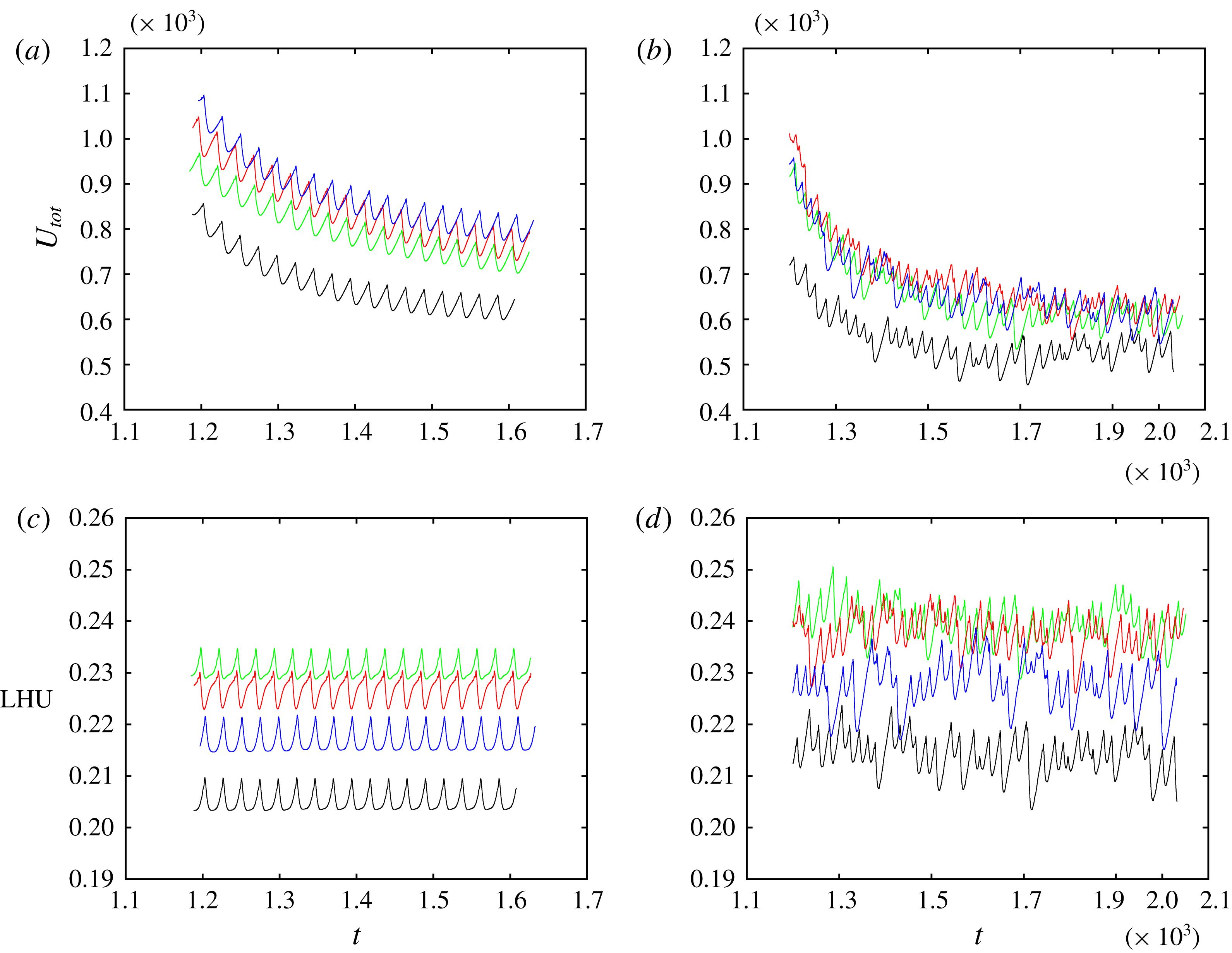
(5.4) (a,b) and liquid holdup LHU (5.5) (c,d). Line types distinguish the different corrugations: flat wall (black), short sinusoidal (green), long sinusoidal (red) and bump-shaped (blue). (a,c) Periodically forced surface waves (cases 2 to 4 in table 1); (b,d) noise-driven surface waves (cases 5 to 9 in table 1).

Figure 9 compares time traces of
 $U_{tot}$
for periodically forced and noise-driven surface waves, different line types representing different corrugation types. For periodically forced waves (figure 9
a), the time traces confirm the trend of figures 4 and 6, i.e.
 $U_{tot}$
is greatest for the bump-shaped corrugations (blue line) followed by the long (red line) and short (green line) sinusoidal corrugations. In principle, the same holds for noise-driven waves (figure 9
b). However, the level of
 $U_{tot}$
is generally lower than for the periodically forced waves and differences between the corrugation types are smaller.
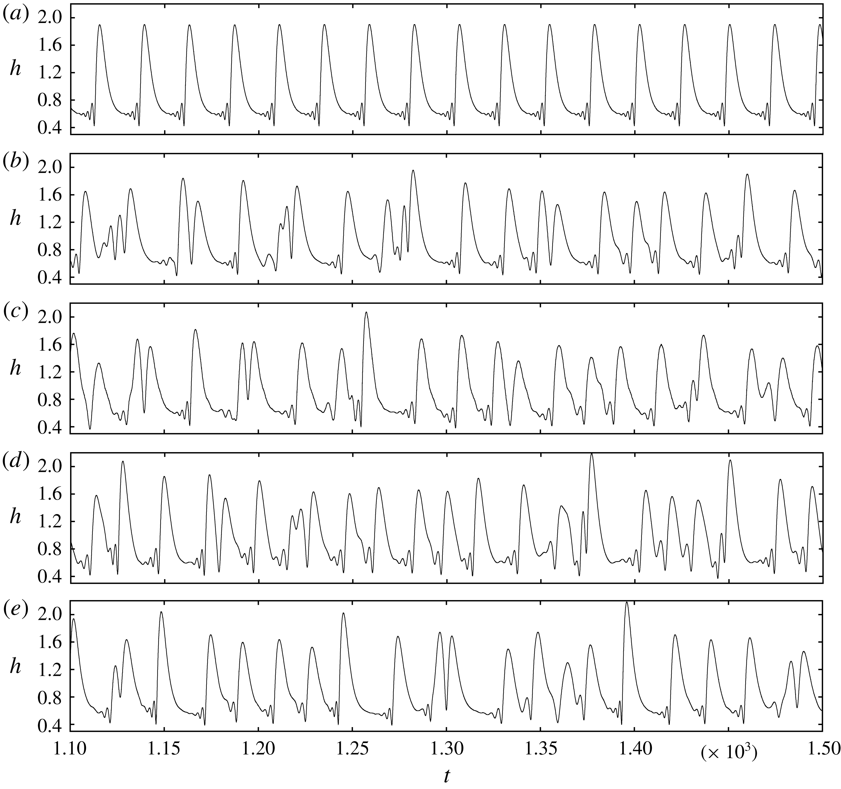
This results from the significantly altered kinematics of the noise-driven surface waves, as evidenced by the film thickness time traces in figure 10. For all corrugation types, the noisy wave spectrum is dominated by waves of smaller amplitude and greater frequency (figure 10 b–e) compared to the periodic waves of case 2 (flat wall, figure 10 a). As a result, the intensification mechanism linked to the large-amplitude solitary waves containing a moving-frame vortex is weakened. Indeed, Rastaturin et al. (Reference Rastaturin, Demekhin and Kalaidin2006) showed for films falling on a flat wall that transfer intensification is diminished when changing from large-amplitude solitary to short waves.
Statistics of noise-driven surface waves (cases 6 to 9, b–e) compared to the flat-wall reference simulation with periodically forced waves (case 2, a). Film thickness time traces at
 $x/L=0.72$
for the different corrugation types. (a) Flat wall, periodic (case 2):
 $\bar{h}=0.91$
,
 $h_{\unicode[STIX]{x1D70E}}=0.43$
,
 $f_{dom}=0.0418$
; (b) flat wall, noise driven (case 6):
 $\bar{h}=0.94$
,
 $h_{\unicode[STIX]{x1D70E}}=0.37$
,
 $f_{dom}=0.0391$
; (c) short sinusoidal corrugation, noise driven (case 7):
 $\bar{h}=0.92$
,
 $h_{\unicode[STIX]{x1D70E}}=0.37$
,
 $f_{dom}=0.0391$
; (d) long sinusoidal corrugation, noise driven (case 8):
 $\bar{h}=0.97$
,
 $h_{\unicode[STIX]{x1D70E}}=0.39$
,
 $f_{dom}=0.0522$
; (e) bump-shaped corrugation, noise driven (case 9):
 $\bar{h}=0.92$
,
 $h_{\unicode[STIX]{x1D70E}}=0.39$
,
 $f_{dom}=0.0391$
. Symbols
 $\bar{h}$
and
 $h_{\unicode[STIX]{x1D70E}}$
denote the time-averaged value and standard deviation of the film thickness
 $h$
, and
 $f_{dom}$
designates the dominant frequency of the wave spectrum as obtained from numerical Fourier transformation.

With one exception, the wall corrugations do not significantly alter the noise-driven wave kinematics. However, for the long sinusoidal corrugation (case 8, figure 10
d), the dominant frequency of the wave spectrum
 $f_{dom}=0.0522$
, which was obtained from numerical Fourier transformation and is reported in the figure caption, is greater than for all other corrugations (figure 10
b,c,e,
 $f_{dom}=0.0391$
) and than for periodically forced waves on a flat wall (figure 10
a,f
 $=0.0418$
). On average, surface waves are thus shortest for this case, explaining why
 $U_{tot}$
in figure 9(b) (red line) is not much greater than for the short sinusoidal corrugation (green line).
Further downstream (outside of our computational domain), we expect the noise-driven wave kinematics to approach those of the periodic wave regime, because short waves will increasingly coalesce to form large-amplitude solitary waves (Chang et al. Reference Chang, Demekhin, Kalaidin and Ye1996b ). Transfer intensification due to the corrugations should then approach the levels observed in figures 4 and 6. Checking this requires simulations on very long domains.
We conclude this section by comparing the liquid holdup LHU
 $$\begin{eqnarray}\displaystyle \text{LHU}=\frac{\displaystyle \int _{0}^{L}h(x)\,\text{d}x}{\displaystyle \int _{0}^{L}(H-f(x))\,\text{d}x} & & \displaystyle\end{eqnarray}$$
for the different wave regimes and wall corrugations. This quantity is represented in figure 9 for the periodic (figure 9 c) and noise-driven (figure 9 d) wave regimes. We see that LHU is systematically greater for the noise-driven wave regimes and is greatest for the short sinusoidal corrugations. As the holdup sets the available cross-section for the counter-current gas flow, this has implications for the pressure drop in the gas, as will be discussed in the following section.
5.3 Pressure drop and flooding
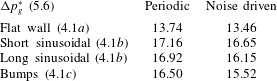
We start by evaluating the gas pressure drop
 $\unicode[STIX]{x0394}p_{g}$
, which we have listed in table 2 for the different corrugations and wave regimes. Therein,
 $\unicode[STIX]{x0394}p_{g}$
has been rescaled in units of the aerostatic pressure drop
 $$\begin{eqnarray}\displaystyle \unicode[STIX]{x0394}p_{g}^{\ast }=\frac{Fr^{2}}{\unicode[STIX]{x1D6F1}_{\unicode[STIX]{x1D70C}}}\unicode[STIX]{x0394}p_{g}. & & \displaystyle\end{eqnarray}$$
The value of
 $\unicode[STIX]{x0394}p_{g}^{\ast }$
is greatest for the short sinusoidal corrugations, which also display the largest liquid holdup (see previous section). By contrast,
 $\unicode[STIX]{x0394}p_{g}^{\ast }$
for the bump-shaped corrugations is smaller than for both sinusoidal corrugations. The bump-shaped corrugations thus produce less of a pressure drop while intensifying scalar transfer to a greater extent. This suggests that they are more efficient than the sinusoidal corrugations.
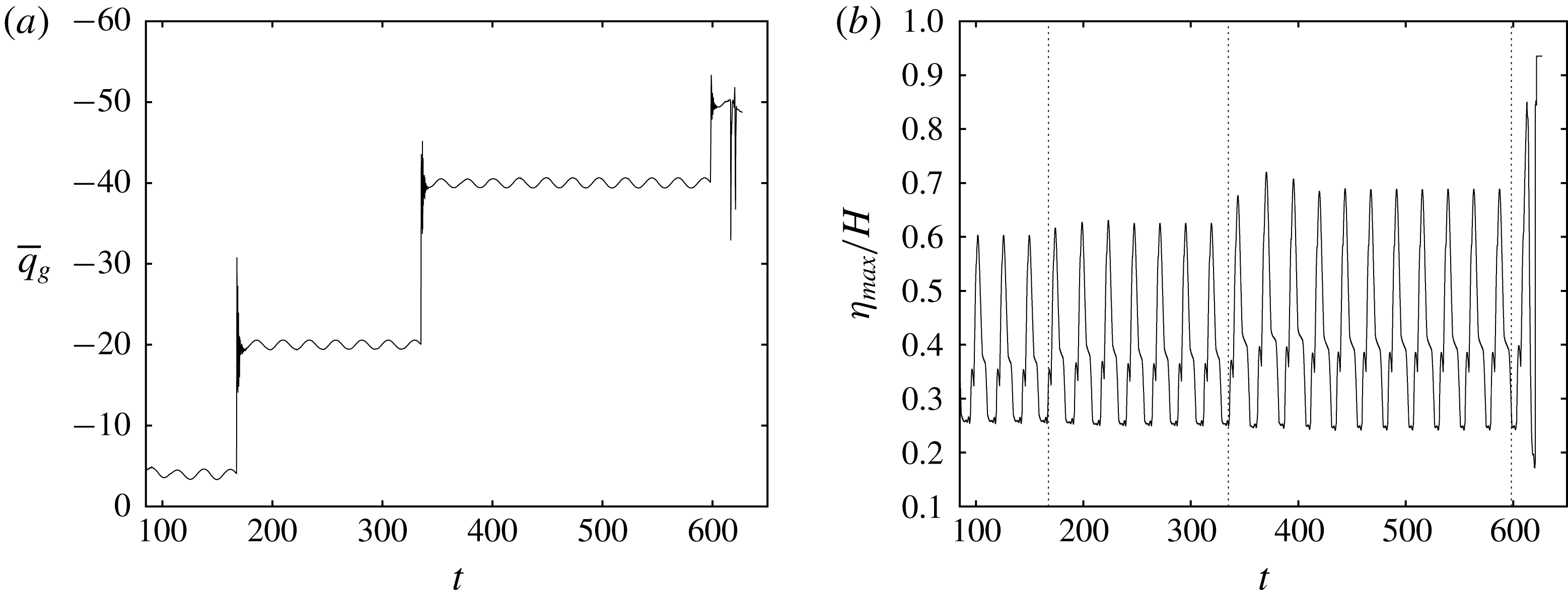
Increasing the counter-current gas flow rate in the simulation with bump-shaped corrugations (case 5, table 1). (a) Spatially averaged flow rate in the gas
 $\bar{q}_{g}=(1/L)\int _{0}^{L}\int _{\unicode[STIX]{x1D702}}^{H}u\,\text{d}y\,\text{d}x$
. The second plateau at
 $\bar{q}_{g}\approx -20$
corresponds to the simulation settings used in §§ 5.1 and 5.2; (b) time trace of the maximum film surface height
 $\unicode[STIX]{x1D702}_{max}$
(open circles in figure 12
a) near the second corrugation bump (
 $0.36\leqslant x/L\leqslant 0.46$
). At the latest time shown, the film has flooded the channel around the third corrugation bump (figure 12
b).

Time-averaged gas pressure drop
 $\unicode[STIX]{x0394}p$
for different wall corrugations and wave regimes (cases 2–9, table 1) rescaled in units of the aerostatic pressure drop:
 $\unicode[STIX]{x0394}p_{g}^{\ast }=\unicode[STIX]{x0394}p_{g}Fr^{2}/\unicode[STIX]{x1D6F1}_{\unicode[STIX]{x1D70C}}$
(5.6).

However, these bumps generate a bottleneck for the gas flow every time a wave hump passes over them. This can trigger the localised flooding of the channel when the counter-current gas flow is increased. We demonstrate this in figures 11 and 12 based on an additional simulation of case 5, where we have incrementally increased the gas velocity by varying
 $q_{g}$
in the boundary condition (2.9) from
 $q_{g}=-4$
to
 $q_{g}=-50$
(simulations in §§ 5.1 and 5.2 were performed with
 $q_{g}=-20$
).
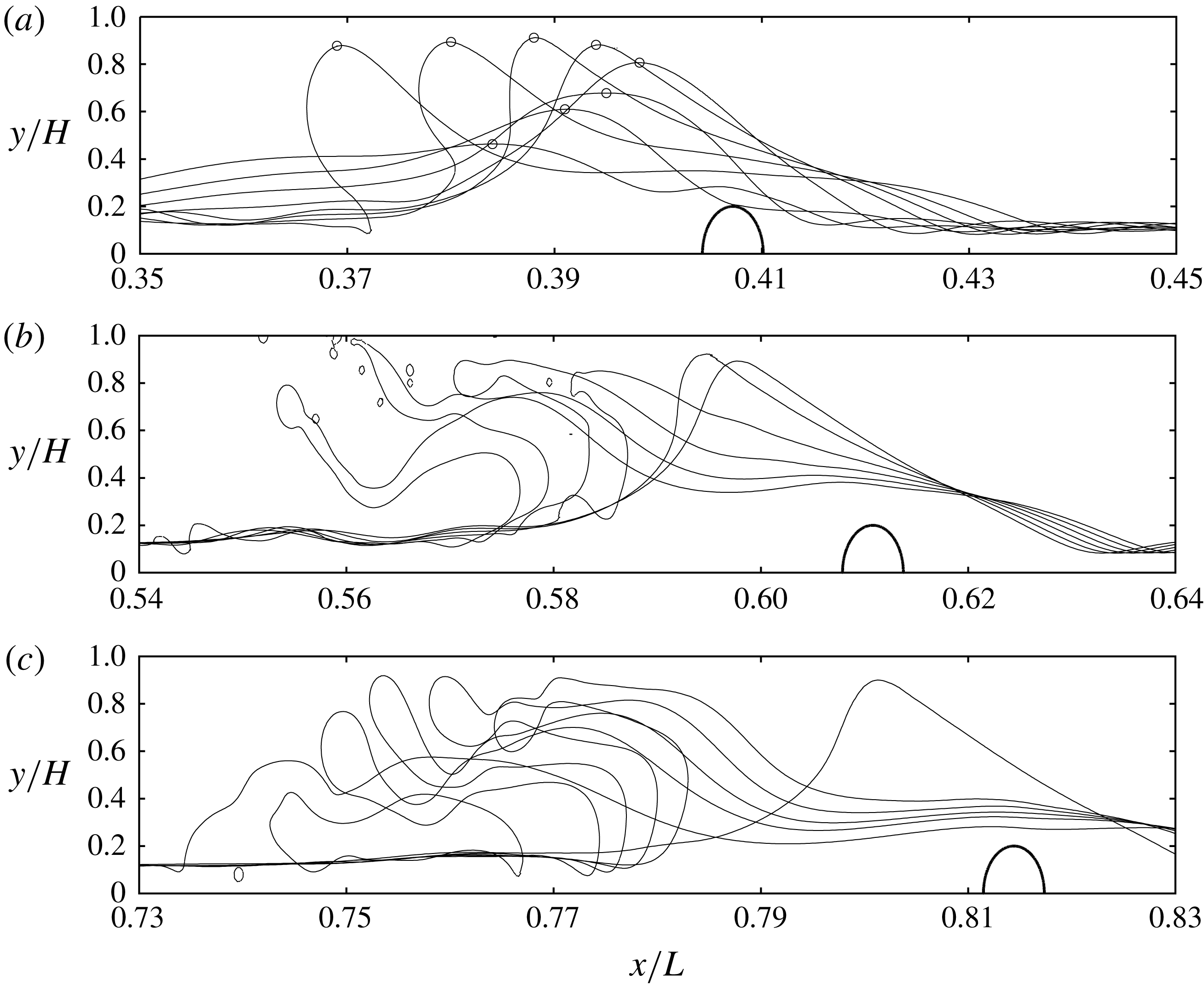
Cascaded flooding of the channel following the last increase in counter-current gas flow rate in figure 11(a). Evolution of film surface profiles at the second, third and fourth corrugation bump. (a) Second bump:
 $607.35\leqslant t\leqslant 613.83$
. Open circles mark maximal film height plotted in figure 11(b); (b) third bump:
 $616.22\leqslant t\leqslant 617.66$
; (c) fourth bump:
 $620.53\leqslant t\leqslant 622.92$
.

Figure 11(a) shows the time trace of the gas flow rate averaged over the entire computational domain and figure 11(b) represents the corresponding time trace of the maximal film surface height in the vicinity of the second corrugation bump. Following the fourth stepwise augmentation of the gas flow rate, an exponential increase of the wave height is observed.
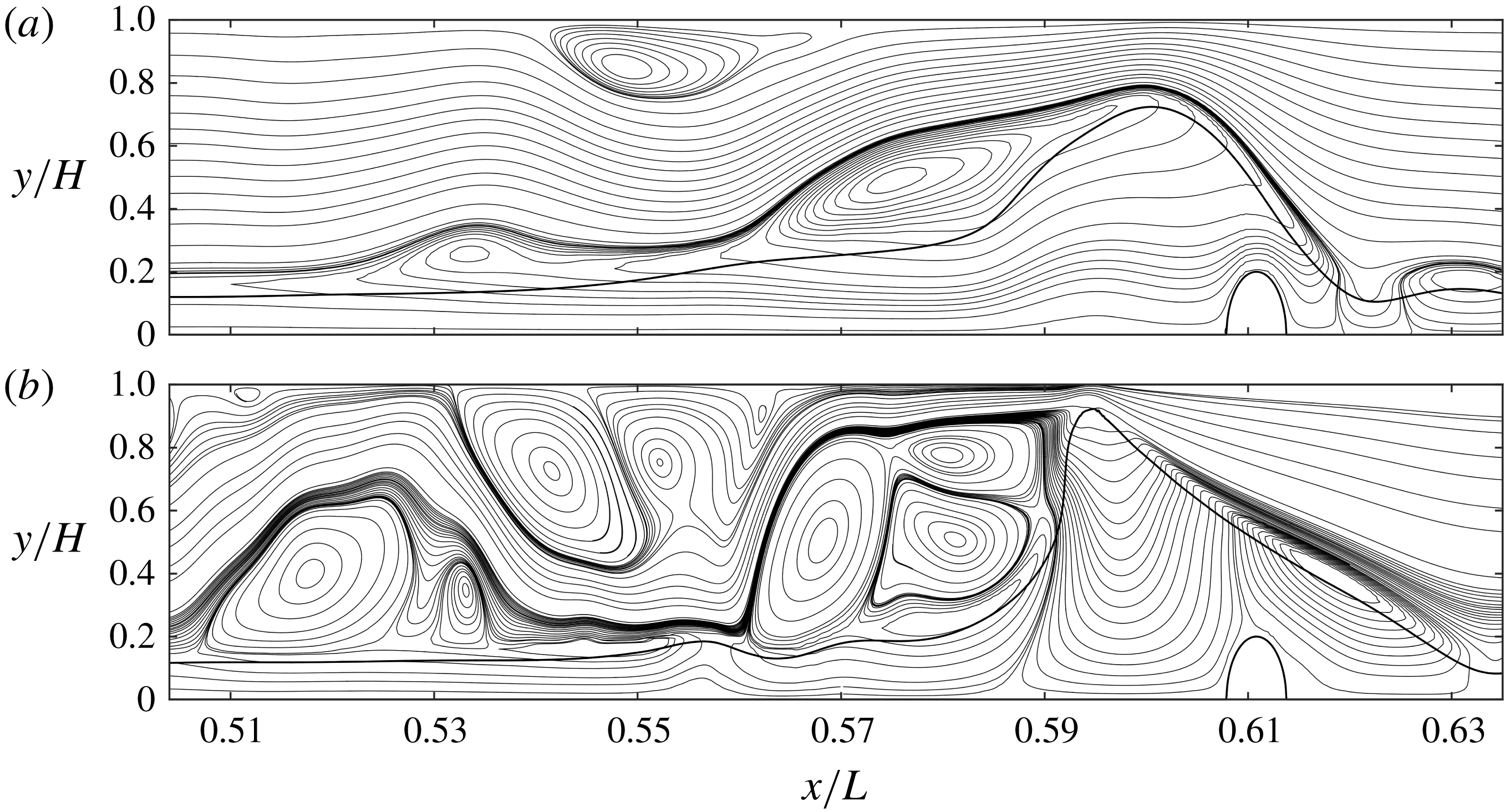
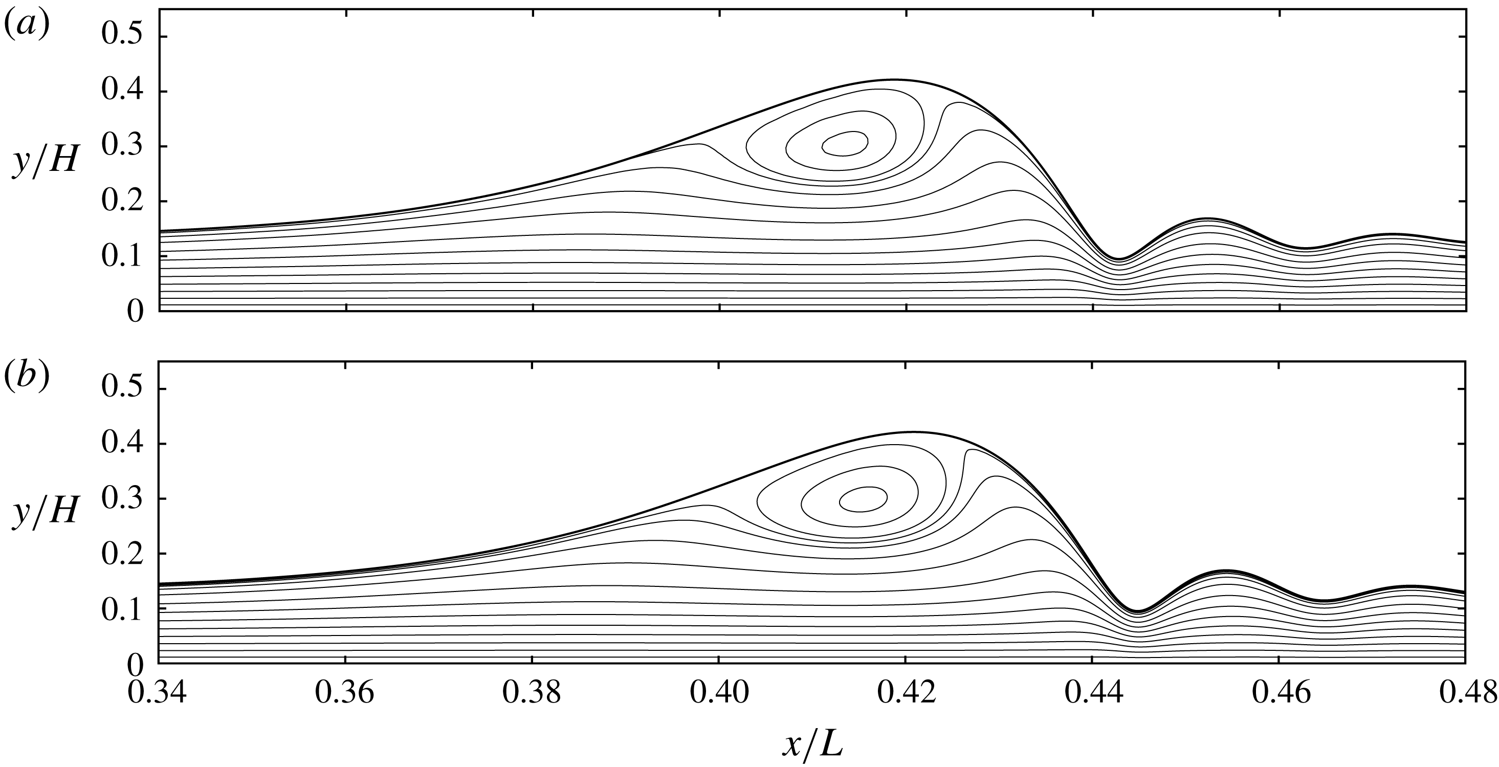
Figure 12 shows that this coincides with a cascade of flooding events at the last three corrugation bumps. The supplementary movie 4 shows the flooding cascade in action and movie 5 shows a close-up view of the flooding event at the third bump (figure 12 b). Leading up to this event, the continuously growing wave hump severely constricts the gas flow and this produces a large number of vortices in the upstream region into which the gas expands. This is shown in figure 13, where streamlines in the wall-fixed reference frame have been plotted at two characteristic time points. Of course, our numerical results do not constitute a fully fledged investigation of flooding. This would require a detailed validation with corresponding experiments. We simply demonstrate that wall corrugations may favour flooding events.
6 Conclusion
We have performed numerical simulations of scalar transfer through the mobile surface of a wavy falling liquid film flowing down a corrugated substrate in interaction with a strongly confined counter-current gas flow. Three different corrugation geometries were considered (see figure 2), and we have contrasted periodically forced versus noise-driven wave regimes (through appropriate inlet forcing) as well as transport regimes of moderately dominant (
 $Pe=459$
) versus strongly dominant (
 $Pe=4590$
) convection by varying the Péclet number
 $Pe$
. Our simulations have yielded the following findings.
Wall corrugations cause a significant additional transfer enhancement, leading to a 30 per cent reduction of the exchange length required to transfer a fixed amount of transported scalar (figures 4 and 6). This can be achieved with different types of corrugations, which act on different wave-induced intensification mechanisms. Sinusoidal corrugations cause a rapid and repetitive extrusion of scalar plumes from the free-surface layer forming at the film surface, every time a wave passes over the downstream slope of a corrugation bump (figure 5). We have explained the underlying mechanism, which is linked to a corrugation-induced periodic variation of the wave celerity.
Streamlines in the wall-fixed reference frame at two characteristic time points leading up to the flooding event at the third corrugation bump (shown in figure 12
b). The thick solid line represents the film surface. Gravity, which drives the liquid film, points from left to right, while the gas flows from right to left (see figure 1). Continued growth of the wave hump leads to a severe constriction of the gas flow, causing the formation of a large number of vortices behind the wave. (a)
 $t=614.45$
; (b)
 $t=616.44$
.

Isolated bump-shaped corrugations allow to intermittently disrupt large-amplitude solitary waves travelling on the film and the moving-frame vortices they contain. Such vortices are known to greatly intensify scalar transfer by compressing the free-surface layer at the back of the wave. However, this mechanism breaks down once the fluid within the vortex is saturated. Adequately spaced (approximately at the separation of the solitary waves) corrugation bumps counteract this natural decay by causing a redistribution of liquid within the wave hump, allowing the moving-frame vortex to replenish with fresh liquid, thus reinitiating the intensification mechanism (figures 7 and 8).
The above effects were observed for strongly dominant convection (
 $Pe=4590$
), which is representative of mass transport. By contrast, no significant corrugation-induced transfer intensification was observed for moderately dominant convection (
 $Pe=459$
), which is representative of heat transport. Maximal intensification was observed for periodically forced surface waves, noise-driven surface waves exhibiting smaller amplitudes associated with weaker moving-frame vortices. In one case, sinusoidal wall corrugations were found to significantly shift the wave spectrum of noise-driven waves compared to that for a flat-wall situation, leading to a lesser transfer intensification (figures 9 and 10).
Among the studied corrugations, the isolated bumps generate the smallest liquid holdup and gas pressure drop. As they also cause a slightly greater transfer intensification than the sinusoidal corrugations, they seem to be a more efficient choice. However, they can trigger flooding events in the strongly confined geometry considered here when the gas velocity is significantly increased. We have checked this by identifying the critical gas flow rate for the onset of flooding (figures 11 and 12). Having said this, the studied confinement is extreme (the channel height is less than five times the mean film thickness) and thus the determined flooding onset is a very conservative limit. In other words, the risk of flooding can be averted by moderately reducing the confinement and this would not diminish the transfer intensification produced by the bump-shaped corrugations.
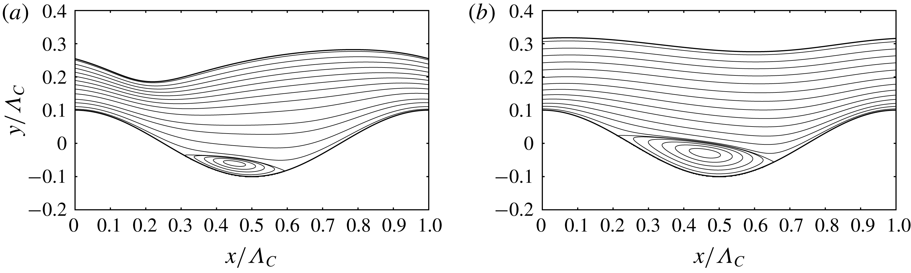
Validation of the numerical code employed: falling liquid film flowing over a deep sinusoidal corrugation inclined at
 $8$
degrees to the horizontal. Conditions correspond to the two experiments reported in figures 3(b) and 3(d) of Wierschem et al. (Reference Wierschem, Pollak, Heining and Aksel2010). (a)
 $Re=16.10$
,
 $\bar{h}/\unicode[STIX]{x1D6EC}_{C}=0.244$
; (b)
 $Re=47.95$
,
 $\bar{h}/\unicode[STIX]{x1D6EC}_{C}=0.297$
. The code accurately predicts the shape of the film surface as well as the size of the separation eddy forming in the corrugation trough.

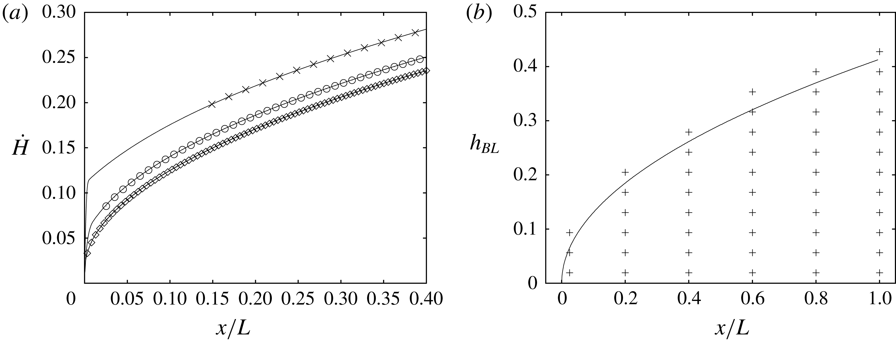
Grid dependence analysis based on case 1 in table 1:
 $Re=15$
,
 $Pe=4590$
. (a) Profiles of the convection rate
 ${\dot{H}}$
(5.1) for three grid resolutions. Only a fraction of the domain length is represented to focus on the inlet. Solid lines correspond to numerical data and symbols to the analytical solution (5.2), which is superimposed onwards from where the free-surface layer is sufficiently resolved and evaluated at streamwise positions corresponding to every 80th grid point. Crosses: coarser grid
 $\unicode[STIX]{x1D6E5}=H/2^{6}$
; open circles: reference grid
 $\unicode[STIX]{x1D6E5}=H/2^{7}$
(employed in § 5); diamonds: finer grid
 $\unicode[STIX]{x1D6E5}=H/2^{8}$
; (b) analytical profile of the free-surface layer thickness
 $h_{BL}=(8/3)^{1/2}\sqrt{x/Pe}$
and reference grid (
 $\unicode[STIX]{x1D6E5}=H/2^{7}$
) at six selected
 $x$
-positions.

Acknowledgements
This work was supported by the ANR wavyFILM project, grant ANR-15-CE06-0016-01 of the French Agence Nationale de la Recherche. Preliminary work was supported by the CNRS institute INSIS through project DYNAFILM. The author acknowledges fruitful discussions with C. Ruyer-Quil.
Supplementary movies
Supplementary movies are available at https://doi.org/10.1017/jfm.2018.851.
Appendix A. Comparison with Wierschem et al. (Reference Wierschem, Pollak, Heining and Aksel2010)
For validation of the employed code, we have simulated the two experiments reported in figure 3(b,d) of Wierschem et al. (Reference Wierschem, Pollak, Heining and Aksel2010), which constitute well established test cases (see e.g. review by Aksel & Schörner (Reference Aksel and Schörner2018)). They concern a film of silicone oil flowing over a deep sinusoidal corrugation inclined at 8 degrees to the horizontal at different values of the Reynolds number. Figure 14 shows the results of our simulations. Therein, figure 14(a,b) should be compared directly with figure 3(b,d) in Wierschem et al. (Reference Wierschem, Pollak, Heining and Aksel2010). Agreement with the experiments is good. In particular, our simulation accurately predicts the shape of the film surface and the size of the separation eddy forming in the corrugation trough. For the lower Reynolds number value (figure 14 a), the eddy is smaller and the film surface minimum lies upstream of it, as opposed to the second case (figure 14 b), where it lies on the downstream side of the eddy.
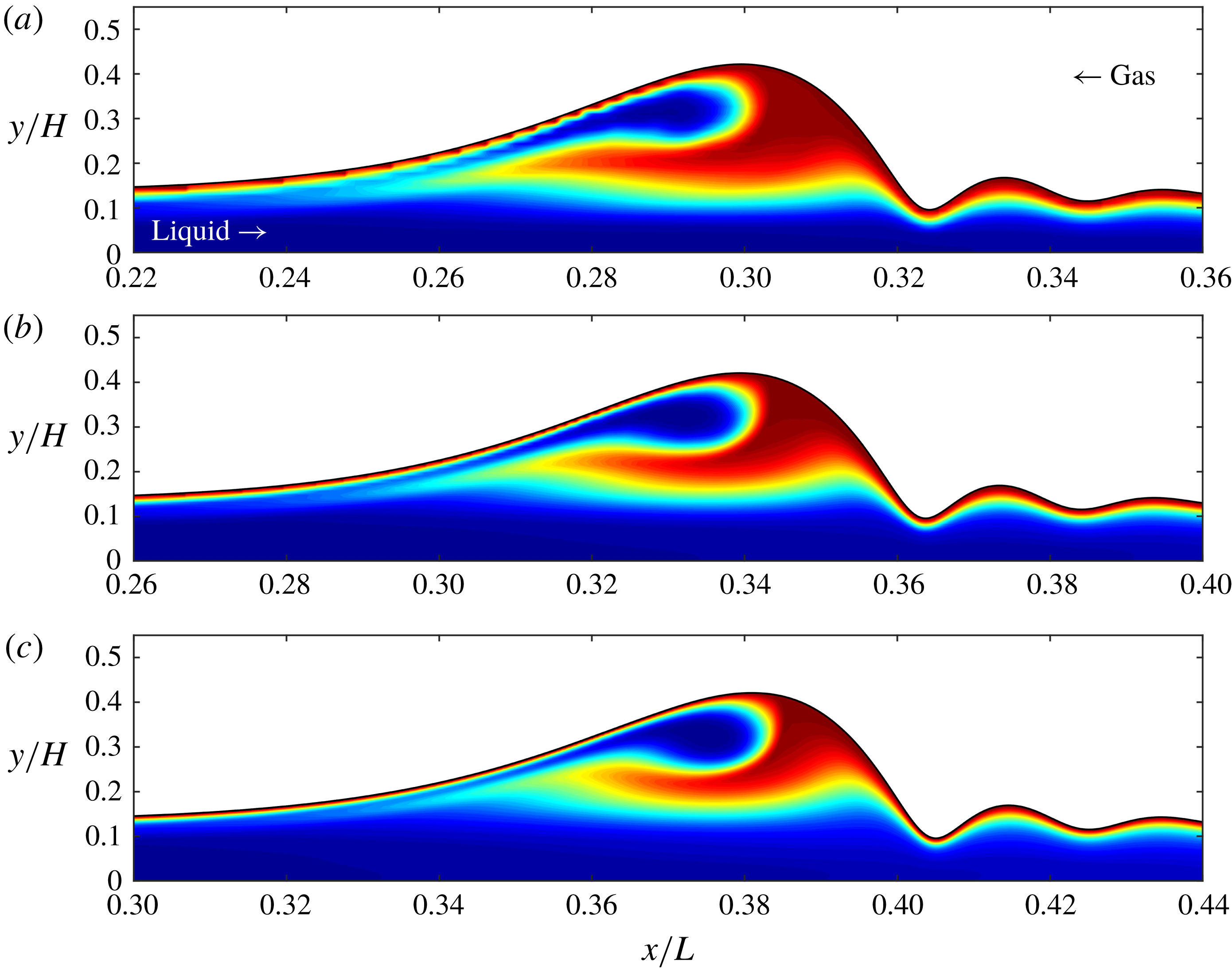
Grid dependence analysis based on case 2 in table 1:
 $Re=15$
,
 $f=0.0418$
,
 $Pe=4590$
. The three panels show the field of the scalar
 $\unicode[STIX]{x1D6E9}$
within a surface wave that has almost reached its saturated shape (blue:
 $\unicode[STIX]{x1D6E9}=0$
; red:
 $\unicode[STIX]{x1D6E9}=1$
). Time points for evaluation are chosen such that the scalar plume in all three cases has just about reached the wave back. (a) Coarse grid:
 $\unicode[STIX]{x1D6E5}=H/2^{6}$
; (b) reference grid employed for all simulations in table 1:
 $\unicode[STIX]{x1D6E5}=H/2^{7}$
; (c) fine grid:
 $\unicode[STIX]{x1D6E5}=H/2^{8}$
. The minimal film thickness (at the capillary trough) is resolved by respectively 6, 12 and 24 cells.

Flow field within the surface wave represented in figure 16(b,c), after it has reached a stationary travelling state (the two data sets are shown at the same time point). The two plots represent streamlines in the wave-fixed reference frame, which is translated at the wave celerity
 $c$
. (a) Reference grid:
 $c=1.930$
; (b) fine grid:
 $c=1.925$
.

Appendix B. Grid dependence analysis
We have performed a grid dependence analysis for two of the simulations reported in table 1: case 1 (flat wall and flat film), and case 2 (flat wall and periodically forced waves). In both cases, we have performed simulations for strongly dominant convection (
 $Pe=4590$
) with a coarser (
 $\unicode[STIX]{x1D6E5}=H/2^{6}$
) and a finer (
 $\unicode[STIX]{x1D6E5}=H/2^{8}$
) grid, in addition to the simulations with the reference resolution used throughout this work (
 $\unicode[STIX]{x1D6E5}=H/2^{7}$
). As the time step is dynamically adapted to satisfy
 $Co\leqslant 0.8$
in each cell, it is refined to the same extent as the spatial resolution in the respective runs, i.e. by a factor of 2 each time. The code has been demonstrated to exhibit second-order convergence both in space and time (Popinet Reference Popinet2003, Reference Popinet2009).
Figure 15 shows the results for case 1. Figure 15(a) represents the convection rate profile
 ${\dot{H}}(x)$
(5.1) for the three resolution variants (solid lines) onto which the analytical solution (5.2) has been superimposed (symbols). Very near the inlet, any numerical simulation based on spatial discretisation inevitably under-resolves the free-surface layer. Consequently, the analytical profiles in figure 15(a) have been superimposed only in the region where the free-surface layer is sufficiently resolved by the respective simulations. This was done by anchoring the analytical solution at the most-upstream point on the simulated profiles onwards from which
 ${\dot{H}}(x)$
obeys the analytical spatial growth
 ${\dot{H}}(x)\propto (x/Pe)^{1/2}$
. The distance of this point from the inlet is a good measure for the state of convergence of the simulations (better than the vertical offset of the
 ${\dot{H}}(x)$
curves, which is mainly inherited from the inevitable under-resolution at the inlet). This distance is quite long for the coarse grid (crosses) but very short for the fine (diamonds) and reference (circles) grids. In the case of the reference grid, it represents only 2.5 per cent of the entire domain length (note that figure 15(a) represents only 40 per cent of the domain length). Figure 15(b) represents the actual profile of the analytical free-surface layer thickness, plus signs marking cell centres of the reference grid at six selected streamwise positions.
Figure 16 shows results for case 2. The different panels display the scalar field within a surface wave for the three grid resolutions. Although there is still a small difference between the fine (figure 16 c) and reference simulations (figure 16 b), the fine result does not exhibit any fundamentally different features. We thus conclude that the reference simulation is sufficiently resolved for the purpose of our study. The small difference that does exist between figures 16(b) and 16(c) mainly stems from the inevitable under-resolution of the free-surface layer very near the liquid inlet, where the free-surface layer thickness is extremely small (see discussion above). Indeed, the surface wave shown in figure 16(b,c) is still at an early stage of development, carrying with it the imprint of the conditions near the inlet. Meanwhile, the hydrodynamics within the wavy film is virtually insensitive to the grid resolution. This is shown in figures 17(a) (reference grid) and 17(b) (fine grid), representing streamlines in the wave-fixed reference frame after the surface wave has reached a travelling state (this is required to draw the entire flow field in the same moving frame). Only very small differences in the streamline pattern can be observed, with a wave celerity difference of just 0.26 % (see caption of figure 17).