

Introduction
According to FAO’s broader estimate, about 25 million people in Southeast Asia are directly dependent on forests (Ma Reference Ma1999), and it has also been reported that 1.5 to 2 million people in Myanmar are directly or indirectly reliant on shifting cultivation (Hlaing Reference Hlaing2004). Shifting cultivation, also known as slash-and-burn agriculture and called ‘Shwe Pyaung Taungya’ in the Myanmar language (Thet and Tokuchi Reference Thet and Tokuchi2020), is a traditional system seasonal crop production practiced mainly in tropical regions (Fox et al Reference Fox, Truong, Rambo, Tuyen, Cuc and Leisz2000; Mertz et al Reference Mertz, Leisz, Heinimann, Rerkasem and Thiha2009; Van Vliet et al Reference Van Vliet, Mertz, Heinimann, Langanke, Pascual and Schmook2012) and is characteristic of traditional farming in Southeast Asia (Jensen Reference Jensen1966; Spencer Reference Spencer1966; Christianty Reference Christanty and Marten1986). This method is defined by the rotation of land use between plots rather than the rotation of crops on the same plot (Marak et al Reference Marak, Kumar, Kundu, Dutta, Pebam and Chattoraj2023). It starts with the clearing and burning of the existing vegetation, followed by a short cropping period of 1 to 3 years. Afterward, cultivation moves to another plot, while the old plot is left fallow for a long period, typically between 5 and 20 years, allowing natural vegetation to regenerate (Fox et al Reference Fox, Truong, Rambo, Tuyen, Cuc and Leisz2000).
Although this practice may offer agricultural benefits, short-term rotation and large-scale expansion into old-growth forests can lead to degradation and fragmentation, with intensified practices further threatening biodiversity (Borah et al Reference Borah, Gilroy, Evans and Edwards2022). Despite this, our understanding of how biodiversity responds throughout the full cycle of shifting cultivation from active farmland to regenerating fallows and mature forests remains limited (Raman et al Reference Raman, Rawat and Johnsingh1998), particularly regarding changing patterns of rotation and fallow periods (Mertz et al Reference Mertz, Bruun, Jepsen, Ryan, Zaehringer and Hinrup2021).
In Myanmar, shifting cultivation has been practiced for centuries or more, especially in hilly regions inhabited by ethnic groups (such as Kachin, Kayah, Karen, Chin, and Shan), and it continues to be practiced in various parts of the country today (Hlaing Reference Hlaing2004; Htun Reference Htun2007).
Tropical secondary forests may require at least 48 years to recover approximately 80% of the species richness found in old-growth forests (Norgrove and Beck Reference Norgrove and Beck2016). Traditionally, fallow periods in shifting cultivation ranged between 20 and 30 years (Spencer Reference Spencer1966), but in recent decades, they have often been shortened to less than five years in some regions, such as Nagaland and other upland areas of Myanmar, where cultivation cycles used to range from 6 to 27 years (Borah et al Reference Borah, Evans and Edwards2018). This reduction in fallow periods is largely driven by population growth and the resulting pressure on land for agricultural use (Ramakrishnan and Patnaik Reference Ramakrishnan and Patnaik1992; Schmidt-Vogt et al Reference Schmidt-Vogt, Leisz, Mertz, Heinimann, Thiha and Messerli2009). As shifting cultivation remains a common land-use practice in many upland areas of Myanmar, it is important to understand how shifting cultivation and different stages of abandoned land affect species and their habitats.
The Green Peafowl Pavo muticus is classified as Endangered, primarily due to pressures from hunting and extensive habitat loss driven by large-scale agricultural development (BirdLife International 2014). Sukumal et al (Reference Sukumal, Dowell and Savini2020) reported that the species is largely restricted to dry forests and has experienced substantial habitat and population declines across mainland Southeast Asia. In Myanmar, recent studies have confirmed its presence in central Myanmar, the Bago Yoma Range (Win et al Reference Win, Sukumal, Shwe and Savini2023), southern Shan State (Shwe et al Reference Shwe, Sukumal, Oo, Dowell, Browne and Savini2021), and the Indawgyi Biosphere Reserve (Sukumal et al in preparation). In addition, Aung et al (Reference Aung, Win and Moses2013) reported the presence of this species in the dry forests at the base of the Rakhine Yoma Mountain Range in west-central Myanmar. These landscapes typically comprise a mosaic of shifting cultivation fields, natural forest and abandoned land at different stages of regrowth, which may provide important habitats for the Green Peafowl. Unfortunately, the area is also experiencing increasing human activities that place growing pressure on natural habitats, highlighting the importance of understanding how traditional farming practices, such as shifting cultivation, affect the species.
Green Peafowl have shown some adaptability to low-intensity, multi-crop agricultural systems situated near their natural habitats (Shwe et al Reference Shwe, Sukumal, Oo, Dowell, Browne and Savini2021); however, they remain highly vulnerable to intensively cultivated landscapes (Sukumal et al Reference Sukumal, McGowan and Savini2015). As with all Galliformes, the species can be considered a good indicator of habitat quality (Savini et al Reference Savini, Namkhan and Sukumal2021), making it valuable for guiding management practices (Grainger et al Reference Grainger, Garson, Browne, McGowan and Savini2018).
Therefore, we aim to investigate how shifting cultivation affects Green Peafowl population density and habitat use by examining how different land-use types, including degraded natural forest, active cultivation plots, and fallow land at different stages of regrowth, influence their landscape use. This study further evaluates the ecological importance of both active cultivation and fallow stages within shifting cultivation systems to inform conservation strategies for preserving Green Peafowl populations in suboptimal habitats in the northern segment of the Rakhine Yoma Mountain Range, west-central Myanmar.
Methods
Survey site
The study was conducted across two survey sites located in Ngape (19°48′ to 20°08′ N, 94°10′ to 94°23′ E) and Minhla Townships (19°48′ to 20°08′ N, 94°10′ to 94°23′ E) in the Magway Region of west-central Myanmar, covering an area of approximately 938.98 km2 within the central dry zone of central Myanmar (Figure 1). The study area lies at a maximum elevation of 700 m above sea level and experiences distinct seasonal variation, with a dry season from February to May and a winter season between November and January. Most precipitation occurs from June to October. The mean annual precipitation is 762 mm. The mean annual temperature is 27.2°C; the warmest month is April, with an average temperature of 31.7°C, while the coldest month is January, with an average temperature of 21.1°C (Thu et al Reference Thu, Li, Zhang, Thang, Soe and Naing2019). The survey area is characterised by mixed teak plantations, Dipterocarp-Indaing and lowland Dipterocarp forests (Dipterocarpus tuberculatus), dry forest (Than-Dahat, composed of Terminalia oliveri and Tectona hamiltoniana), dry thorn forest (scrubland) (FAO 2020), cultivation fields (both permanent and shifting-cultivation systems), and secondary vegetation at various successional stages. In the study area, seasonal crop plantations are dominated by chickpea and pigeon pea, which are widely cultivated across both the southern and northern sites. In addition, small portions of land are used for sesame and paddy cultivation.
Location of the study area comprising two sites: the northern and southern study sites. Black lines represent survey transects, and the black outline delineates the study area boundary. Land-use and land-cover classes include water (blue), degraded natural forest (dark green), fallow land aged 6–10 years (bright green), fallow land <6 years (pale green), active shifting cultivation (cream), and paddy fields (brown).

Figure 1. Long description
The left panel shows a large-scale map of the study area oriented North. A black outline delineates a long, narrow study area stretching from North to South. Two red squares highlight specific focus areas. The Northern Study Site is located at approximately 20 degrees 10 minutes North, and the Southern Study Site is at 19 degrees 50 minutes North. A scale bar at the bottom left indicates 0 to 20 Kilometers.
Two panels on the right provide zoomed-in views of these red squares.
- The top-right panel shows the Northern Study Site with several thick black curved lines representing survey transects scattered across a landscape dominated by bright green fallow land aged 6 to 10 years and dark green degraded natural forest.
- The bottom-right panel shows the Southern Study Site where survey transects are more concentrated in a vertical, parallel arrangement.
The land-cover legend at the bottom identifies six classes.
- Blue represents Water.
- Dark green represents Degraded Natural Forest.
- Bright green represents Fallow Land Aged 6 to 10 Years.
- Pale green represents Fallow Land less than 6 Years.
- Cream represents Active Shifting-cultivation.
- Brown represents Paddy Field.
Density estimates
Species density was estimated using 26 line transects, eight in the northern site and 18 in the southern one (Figure 1). Each transect was 2 km in length and spaced 2 km apart (perpendicular distance), with a 500 m gap between the end of one transect and the beginning of the next (Sukumal et al Reference Sukumal, Thunhikorn and Savini2023). Data were collected during the breeding season from 27 December 2023 to 20 March 2024, when the birds frequently call (Brickle et al Reference Brickle, Cu, Ha, Nguyen and Hoang1998). Only vocal detections were recorded, with calls expected to be heard within 1 km on either side of the transect line. Transects were walked by different observers twice daily, in the morning (06h00–08h30) and in the evening (16h00–18h30), over three consecutive days, for a total of six visits per transect (Sukumal et al Reference Sukumal, McGowan and Savini2015, Reference Sukumal, Dowell and Savini2017). For each detected calling individual, observers recorded the time of the call, its position along the transect, and the estimated angle and distance to the bird. The distance to each calling bird was categorised as 50 m for closer detections and in 100 m intervals for farther distances. Before data collection began, all observers carried out a preliminary survey together to calibrate their distance estimates and reduce observer error (Buckland et al Reference Buckland, Anderson, Burnham, Laake, Borchers and Thomas2001). To increase detection rates, we conducted repeated surveys over more than three consecutive days along the most productive transects, which were mostly located in the southern part of the study area.
We estimated the density of calling male Green Peafowl using distance sampling methods implemented in the program DISTANCE (Buckland et al Reference Buckland, Rexstad, Marques and Oedekoven2015). In the analysis we used the middle point for each bin (i.e. for 50 to 100 m we used 75 m). Detection functions, such as uniform, half-normal, hazard-rate, and negative exponential models with cosine adjustment were examined, and the best model was selected based on the lowest AIC value (Buckland 2001). The analysis was conducted in two stages. First, we estimated the overall density for the entire study area, which encompassed two survey sites: the northern and southern study sites. We then estimated species density separately for the southern study site, where detection rates were higher.
Habitat use
To investigate habitat use by Green Peafowl, five habitat types were classified: (1) active cultivation plots, (2) fallow land less than 6 years old, (3) fallow land aged 6–10 years, (4) paddy fields, and (5) degraded natural forest. Habitat classification was conducted using supervised classification in Google Earth Engine (GEE) based on ground-truth training points and Sentinel-2 Surface Reflectance imagery (COPERNICUS_S2_SR_HARMONIZED). The area of each habitat type was calculated by creating an 800 m buffer on either side of each line transect, corresponding to the maximum distance the species was detected during the survey. Buffer creation and area calculations were performed in ArcGIS 10.8. We recorded the presence of disturbance variables directly along the line transect whenever encountered. The disturbance variables were: (1) forest fire, (2) chainsaw activity (quantified as the total number of chainsaw sounds detected while walking each transect), (3) presence of humans, and (4) presence of dogs. These habitat and disturbance variables were used as predictor variables to assess how anthropogenic pressures influence Green Peafowl habitat use.
At the time of the survey, most shifting cultivation areas were in a cleared and burned stage as part of land preparation for the upcoming cropping season, while others were in a post-harvest stage.
Fallow land less than 6 years old was characterised by a very open vegetation structure, with sparse ground cover, scattered pioneer herbs and shrubs, along with limited recruitment of woody species. Fallow land aged 6–10 years showed noticeably open ground and mid-storey vegetation, with a higher abundance of regenerating woody plants and small trees indicating progression toward early secondary forest development.
In the study area, natural forests have been heavily disturbed over the past decade due to logging and repeated fire events. As a result, the forest structure is degraded and fragmented, with discontinuous patches isolated from one another, few or no large trees remaining, a predominance of small- to medium-sized trees, sparse canopy cover, and a relatively dense understory.
Prior to analysis, all continuous variables were standardised by centering and scaling using two standard deviations to facilitate comparison of parameter estimates among variables and improve model convergence. Pairwise correlations among predictor variables were assessed using Kendall’s rank correlation coefficient, and the correlation matrix was visualised using the corrplot package in R (Wei and Simko Reference Wei and Simko2017). Variables showing strong collinearity (>0.5) were not included in the same model.
To examine the effects of different habitat types and disturbance variables on Green Peafowl abundance, Generalised Linear Mixed Models (GLMMs) with a Poisson error distribution and log-link function were fitted using the glmmTMB package (Brooks et al 2017). The number of Green Peafowl individuals detected during each survey was used as the response variable. Survey effort was incorporated as an offset term [log(Effort)] to account for differences in sampling effort among surveys. Transect identity (Transect.No) was included as a random effect to account for repeated surveys and unexplained variation among transects.
To select the best model, a null model containing only the offset term and random effect was fitted. A global model including all habitats and disturbance variables was then constructed. Subsequently, a series of candidate models were developed by removing less informative variables while retaining most effective predictors (Table 3). Multicollinearity in candidate models was further evaluated using variance inflation factors (VIFs) calculated with the performance package. Candidate models were compared using Akaike’s Information Criterion (AIC), and the model with the lowest AIC value and highest AIC weight was selected as the best-supported model. When the best-supported model exhibited a Delta AIC value of less than 2, model averaging was conducted across all candidate models with Delta AIC values below 2.
The final model was also evaluated for outliers, overdispersion, and zero inflation using the DHARMa package (Hartig Reference Hartig2019). All statistical analyses were conducted in R version 4.4.2 (R Core Team Reference Team2025).
Results
Density estimation
A total of 66 detections of calling male Green Peafowl were recorded across the entire study area. Only 2 detections were recorded along 8 transects in the northern study site, while the majority of detections (64) were recorded along 18 transects in the southern study site of the survey area.
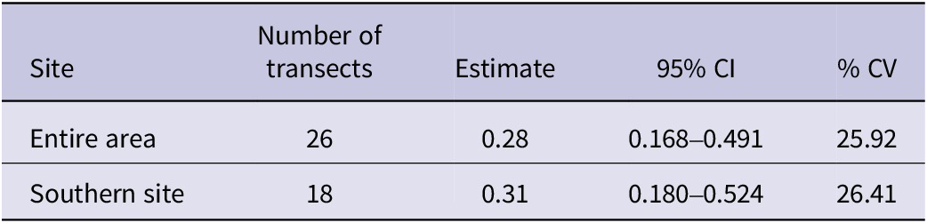
The estimated density of calling males across the entire survey area was 0.29 birds per km2 (95% CI: 0.17–0.49, %CV = 25.92). In the southern study site, where detection rates were higher, the estimated density was slightly greater at 0.31 birds per km2 (95% CI: 0.18– 0.53, %CV = 26.41). Due to the low number of detections in the northern site, density estimation could not be performed. (Table 5)
Variables influencing Green Peafowl habitat use
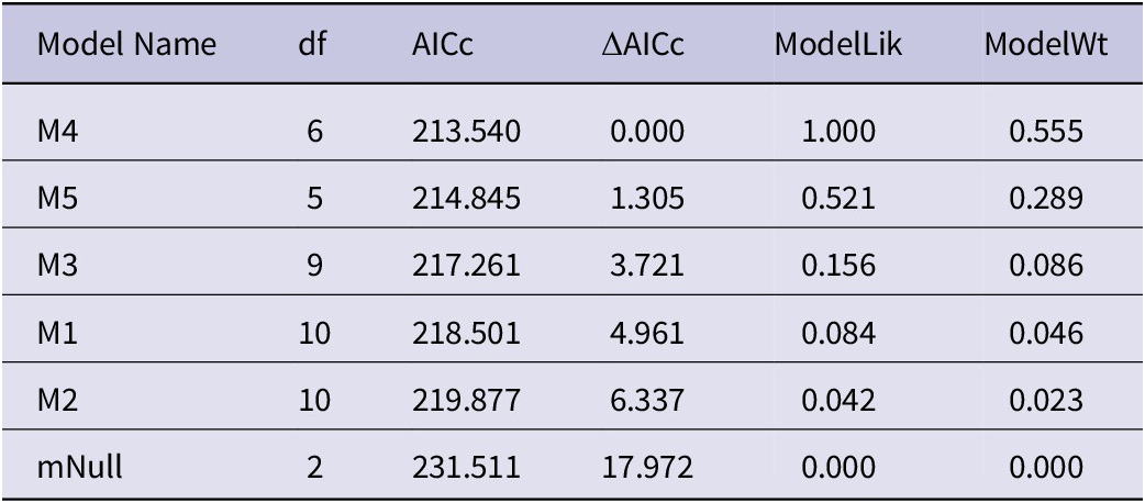
Based on the AICc comparison, the two models with the lowest AICc values, M4 (AICc = 213.54) and M5 (AICc = 214.84), were identified as the most strongly supported models. Both models had Delta AICc values less than 2 and the highest Akaike weights (0.55 and 0.28, respectively). Consequently, model averaging was applied across these two models to obtain the final variable estimates and inference. (Table 1)
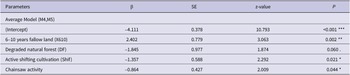
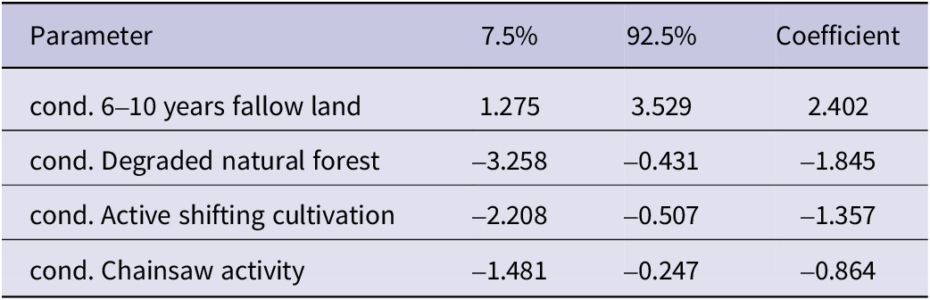
The best-fitting model indicated that Green Peafowl number was significantly influenced by both habitat and disturbance variables. Variable effects were considered significant when the 85% confidence intervals of the model coefficients did not overlap zero ()(Table 4). The variable 6–10 years fallow land (X610) was significantly and positively associated with Green Peafowl numbers ((β = 2.40, 85% CI: 1.27 to 3.52). Active shifting cultivation (Shif) had a significant negative effect on Green Peafowl number (β = −1.35, 85% CI: −2.20 to −0.05), while chainsaw activity was also negatively associated with Green Peafowl number (β = −0.86, 85% CI: −1.48 to −0.24). Degraded natural forest (DF) showed significant negative relationship with Green Peafowl number (β = −1.84, 85% CI: −3.25 to −0.43).(Figure 2, Table 2)
Predicted number of Green Peafowl in response to variables included in the selected model: (a) 6–10 years fallow land (P = 0.0021), (b) degraded natural forest (P = 0.0608), (c) active shifting cultivation (P = 0.021) and (d) chainsaw activity (P = 0.044).
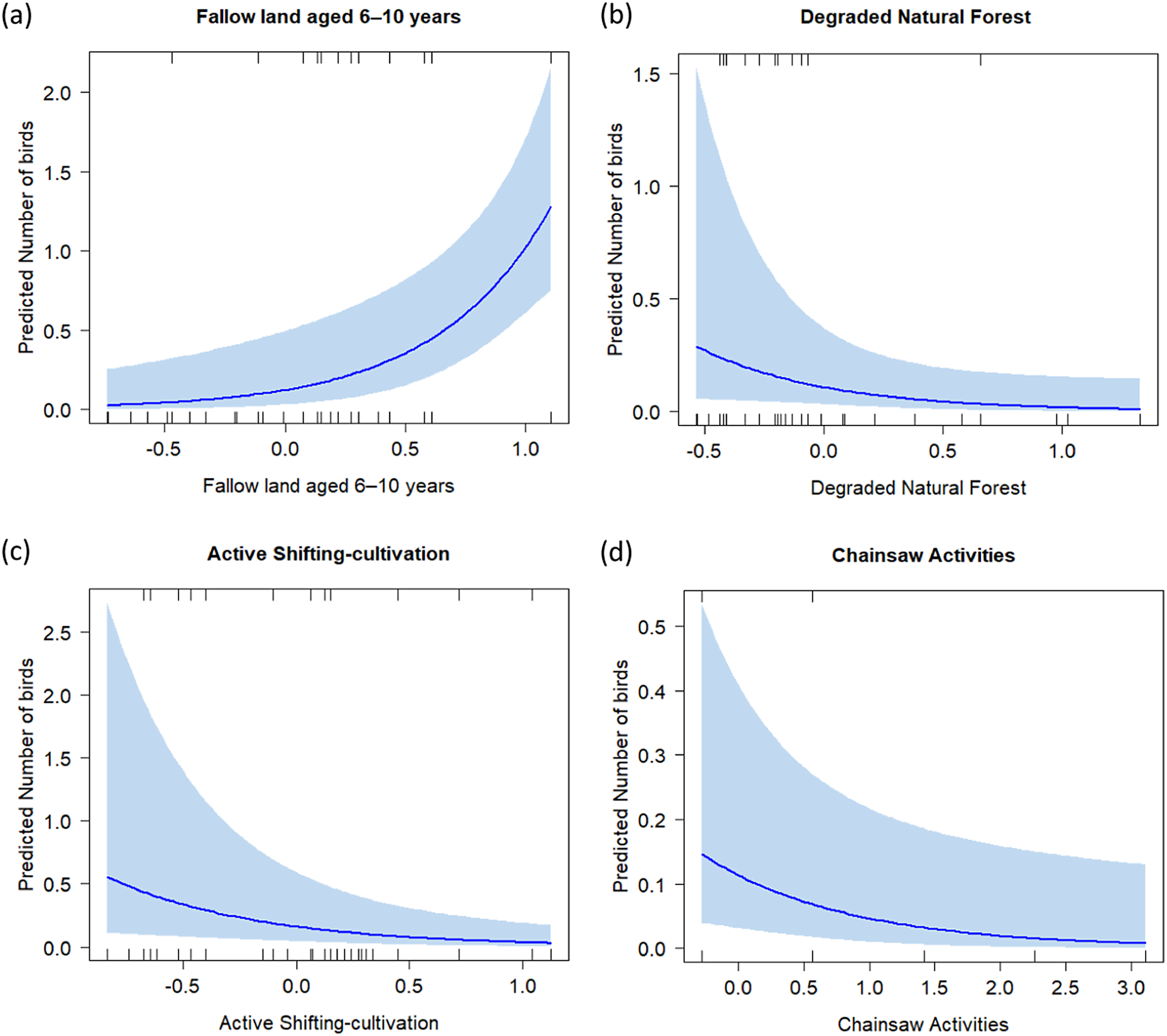
Figure 2. Long description
A four-panel set of line graphs. Each graph shares a Y-axis labeled Predicted Number of birds. Rug plots showing data density are located along the top and bottom inner edges of each frame.
Panel a, Fallow land aged 6 to 10 years. The X-axis ranges from negative 0.5 to 1.0. The blue trend line shows an exponential increase, starting near 0.0 and rising sharply to approximately 1.3 at the right edge. A light blue shaded confidence interval widens as the value increases.
Panel b, Degraded Natural Forest. The X-axis ranges from negative 0.5 to 1.0. The blue trend line shows a shallow exponential decay, starting at 0.3 and leveling off near 0.0. The shaded confidence interval is widest at the left and narrows toward the right.
Panel c, Active Shifting-cultivation. The X-axis ranges from negative 0.5 to 1.0. The blue trend line shows a downward curve starting at 0.5 and approaching 0.0. The shaded confidence interval is very wide at the negative 0.5 mark and tapers significantly as cultivation increases.
Panel d, Chainsaw Activities. The X-axis ranges from 0.0 to 3.0. The blue trend line shows a gradual decline from 0.15 toward 0.0. The shaded confidence interval remains relatively consistent in width across the X-axis.
AICc-based model selection for candidate models. df denotes degrees of freedom, ΔAICc represents the difference from the best-supported model, ModelLik indicates model likelihood, and ModelWt is the Akaike weight

Table 1. Long description
The table consists of six columns: Model Name, d f, A I C c, Delta A I C c, ModelLik, and ModelWt. The rows are ordered as follows:
* M 4: d f 6, A I C c 213.540, Delta A I C c 0.000, ModelLik 1.000, ModelWt 0.555.
* M 5: d f 5, A I C c 214.845, Delta A I C c 1.305, ModelLik 0.521, ModelWt 0.289.
* M 3: d f 9, A I C c 217.261, Delta A I C c 3.721, ModelLik 0.156, ModelWt 0.086.
* M 1: d f 10, A I C c 218.501, Delta A I C c 4.961, ModelLik 0.084, ModelWt 0.046.
* M 2: d f 10, A I C c 219.877, Delta A I C c 6.337, ModelLik 0.042, ModelWt 0.023.
* mNull: d f 2, A I C c 231.511, Delta A I C c 17.972, ModelLik 0.000, ModelWt 0.000.
Results of generalised linear mixed model (GLMMs) examining the effects of habitat types on Green Peafowl occurrence: 1) fallow land < 6 years, 2) fallow land aged 6–10 years, 3) active shifting cultivation, 4) degraded natural forest, and 5) chainsaw activity. The table presents parameter coefficients (β), standard errors (SE), z-values, and significance levels (p-values) for each predictor
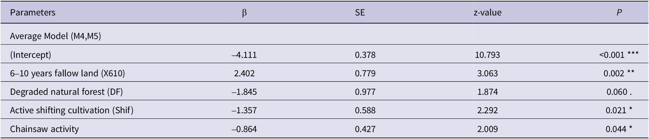
Table 2. Long description
The table consists of five columns: Parameters, beta (beta), S E, z-value, and P.
* Header Row: Parameters, beta, S E, z-value, P.
* Row 1: Average Model (M 4, M 5) serves as a section header.
* Row 2: (Intercept); beta is -4.111; S E is 0.378; z-value is 10.793; P is less than 0.001 (indicated by three asterisks).
* Row 3: 6-10 years fallow land (X 6 10); beta is 2.402; S E is 0.779; z-value is 3.063; P is 0.002 (indicated by two asterisks).
* Row 4: Degraded natural forest (D F); beta is -1.845; S E is 0.977; z-value is 1.874; P is 0.060 (indicated by a dot).
* Row 5: Active shifting cultivation (Shif); beta is -1.357; S E is 0.588; z-value is 2.292; P is 0.021 (indicated by one asterisk).
* Row 6: Chainsaw activity; beta is -0.864; S E is 0.427; z-value is 2.009; P is 0.044 (indicated by one asterisk).
Footnote: One asterisk indicates P less than 0.05; two asterisks indicate P less than 0.01; three asterisks indicate P less than 0.001.
* P<0.05; **<0.01; ***P<0.001
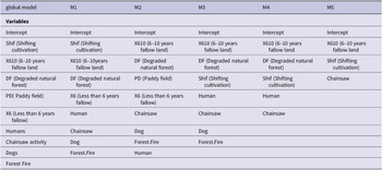
List of variables included in each model
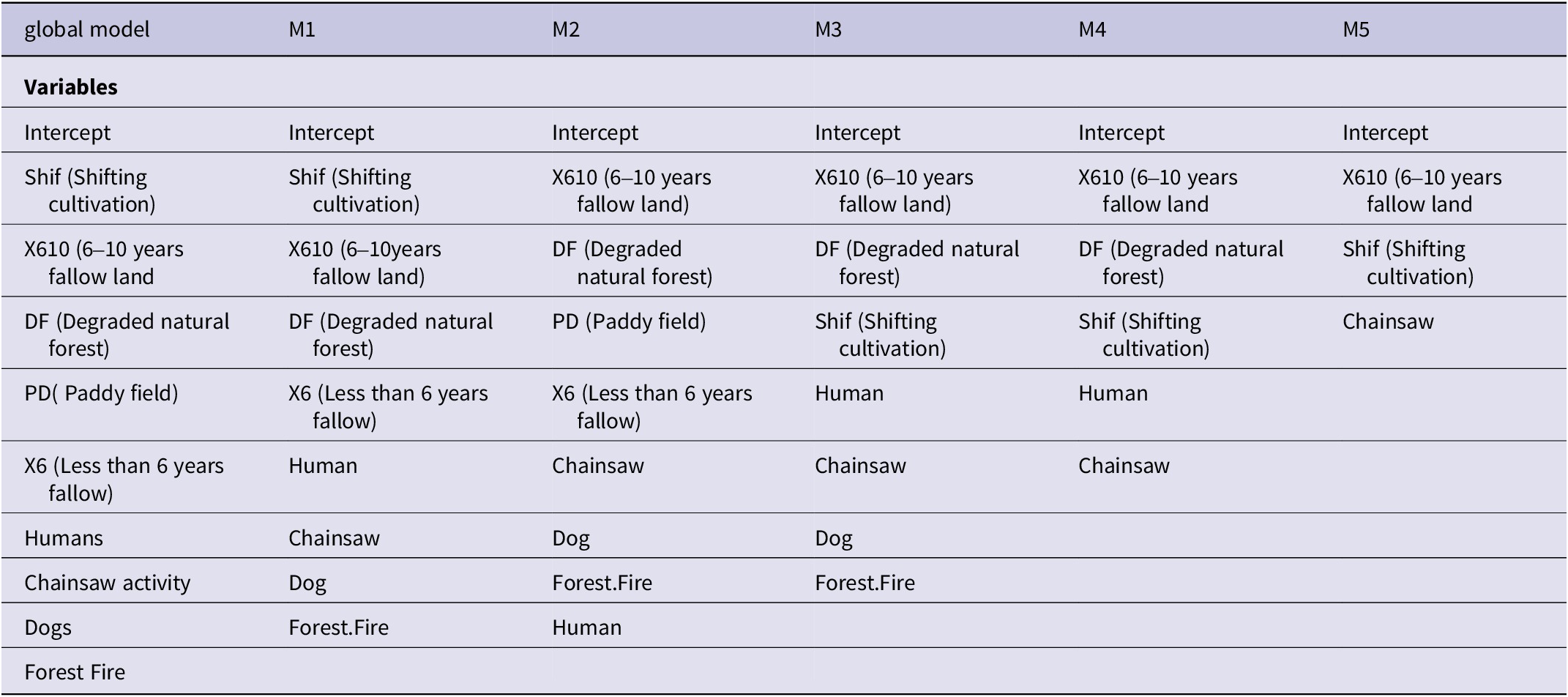
Table 3. Long description
The table consists of six columns representing different statistical models.
* The global model column includes Intercept, Shif (Shifting cultivation), X 6 1 0 (6 to 10 years fallow land), D F (Degraded natural forest), P D (Paddy field), X 6 (Less than 6 years fallow), Humans, Chainsaw activity, Dogs, and Forest Fire.
* Model M 1 includes Intercept, Shif, X 6 1 0, D F, X 6, Human, Chainsaw, Dog, and Forest Fire.
* Model M 2 includes Intercept, X 6 1 0, D F, P D, X 6, Chainsaw, Dog, Forest Fire, and Human.
* Model M 3 includes Intercept, X 6 1 0, D F, Shif, Human, Chainsaw, Dog, and Forest Fire.
* Model M 4 includes Intercept, X 6 1 0, D F, Shif, Human, and Chainsaw.
* Model M 5 includes Intercept, X 6 1 0, Shif, and Chainsaw.
Coefficients of each variable and their 85% confidence intervals from the selected averaged model (M4 and M5). Variables whose confidence intervals did not overlap zero were considered to have a statistically significant effect on Green Peafowl numbers
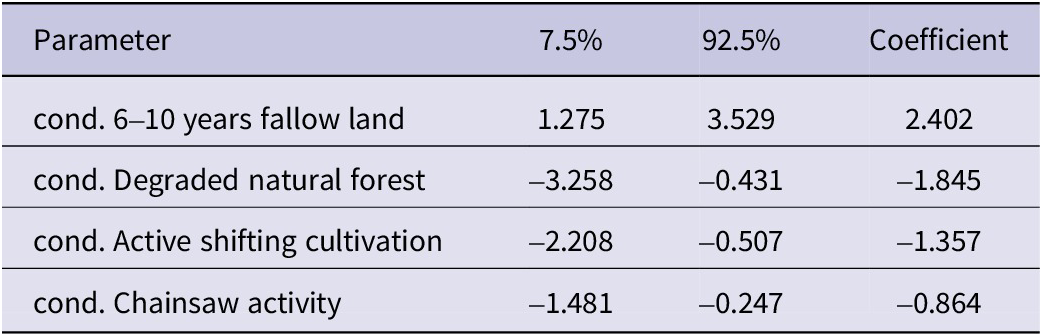
Table 4. Long description
The table consists of four columns: Parameter, 7.5 percent, 92.5 percent, and Coefficient.
* Row 1: cond. 6 to 10 years fallow land. 7.5 percent is 1.275. 92.5 percent is 3.529. Coefficient is 2.402.
* Row 2: cond. Degraded natural forest. 7.5 percent is minus 3.258. 92.5 percent is minus 0.431. Coefficient is minus 1.845.
* Row 3: cond. Active shifting cultivation. 7.5 percent is minus 2.208. 92.5 percent is minus 0.507. Coefficient is minus 1.357.
* Row 4: cond. Chainsaw activity. 7.5 percent is minus 1.481. 92.5 percent is minus 0.247. Coefficient is minus 0.864.
Estimates of Green Peafowl density for the entire study area and the southern study site (Figure 1) using distance sampling. The Table also shows the 95% confidence intervals (CI) and coefficients of variation (%CV) for the abundance estimates
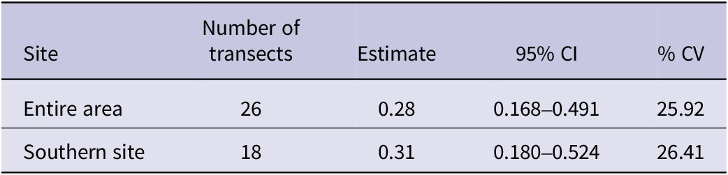
Table 5. Long description
The table consists of five columns and two data rows.
Column headers from left to right are: Site, Number of transects, Estimate, 95 percent C I, and percent C V.
Data rows:
* Entire area: 26 transects, density estimate of 0.28, 95 percent C I of 0.168 to 0.491, and a C V of 25.92 percent.
* Southern site: 18 transects, density estimate of 0.31, 95 percent C I of 0.180 to 0.524, and a C V of 26.41 percent.
Discussion
The estimated density of Green Peafowl across the entire study area was 0.29 calling males per km2, with a slightly higher density of 0.31 calling males per km2 in the southern study site. Although villagers from the northern study site, where eight transects were surveyed, reported frequent encounters with Green Peafowl near the survey area, only two detections were recorded during our surveys. Although we used acoustic detections to reduce potential bias associated with visual surveys, differences in detectability among habitats cannot be excluded. Vegetation structure, topography, background noise and other environmental factors may be partly related to variation in detectability and should be considered when interpreting the observed habitat associations. In addition, the lower density observed in the northern part of the study area might be related to greater human disturbance. Five of the eight transects were located closer to human settlements and the main road connecting Ngape and Sidoktaya townships, where the presence of free-ranging dogs and vehicle traffic may have contributed to the lower number of Green Peafowl detections recorded during surveys. However, given the low number of detections recorded at the northern study site, our data do not allow us to determine whether the observed pattern reflects reduced detectability during the survey period or genuinely lower abundance.
Our estimated densities are considerably lower than those reported from other sites within Myanmar. Shwe et al Reference Shwe, Sukumal, Oo, Dowell, Browne and Savini2021 reported densities of 1.13–2.63 males per km2 in agriculture-dominated landscapes of the Southern Shan Plateau, while Win et al (Reference Win, Sukumal, Shwe and Savini2023) estimated a density of 0.8 calling males per km2 in dry forest mixed with teak in the Bago Yoma range, central Myanmar. Compared to more intact or preferred habitats across Southeast Asia, the density at our study site remains substantially lower, although it exceeds the 0.25 calling males per km2 reported in Yok Don National Park, Vietnam (Sukumal et al Reference Sukumal, McGowan and Savini2015). In Thailand, densities ranged from 1.13 to 11.34 calling males per km2 in Huai Kha Khaeng Wildlife Sanctuary (Sukumal et al Reference Sukumal, Dowell and Savini2017), while a density of 15.82 calling males per km2 was reported in mixed dry-teak forests of northern Thailand (Saridnirun et al Reference Saridnirun, Sukumal, Grainger and Savini2021). In Cambodia, 0.35–1.70 calling males per km2 were recorded in Siem Pang Wildlife Sanctuary and 0.56–1.08 calling males per km2 in Srepok Wildlife Sanctuary (Loveridge et al Reference Loveridge, Kidney, Ty, Eang, Eames and Borchers2017; Tak et al Reference Tak, Crouthers, Sukumal and Chhin2022) and degraded habitats. The density at our site is slightly lower than the 0.39 individuals per km2 recorded in Keo Seima Wildlife Sanctuary, Cambodia (Nuttall et al Reference Nuttall, Griffin, Fewster, McGowan, Abernethy and O’Kelly2022).
The widely differing population densities between our study area and two other study sites in Myanmar may be partly explained by differences in hunting pressure, socio-cultural context, and habitat extent. In our study area, lower conservation awareness and high hunting pressure may contribute to lower population densities, although hunting pressure was not quantified because of insufficient data. The larger population density in the Southern Shan State study area has been suggested to reflect the strong influence of resident Theravada Buddhist clergy and religious beliefs discouraging hunting of Green Peafowl, potentially reducing persecution and supporting population persistence (Shwe et al Reference Shwe, Sukumal, Oo, Dowell, Browne and Savini2021). The higher population density observed in the Bago Yoma range in central Myanmar was associated with the availability of suitable habitat and large forest patches due to well managed teak plantations (Win et al Reference Win, Sukumal, Shwe and Savini2023).
We examined habitat use of Green Peafowl across five habitat types, including human-modified lands and the remaining degraded natural forests within the study area. This approach allowed us to clarify how habitat modification influences peafowl habitat preferences. Our findings revealed that Green Peafowl were more abundant in intermediate successional habitats, particularly 6–10 years old fallow lands. This finding may be associated with the heterogeneous vegetation structure of these habitats, which is likely to provide a combination of vegetation cover, foraging opportunities, and open ground that may be favourable for the species. However, these mechanisms were not directly measured in this study and should therefore be considered possible explanations for the observed pattern. This pattern highlights the species’ ecological flexibility in utilising modified habitats, especially where secondary forests and fallow lands occur near remnant old-growth forests (Raman et al Reference Raman, Rawat and Johnsingh1998; Borah Reference Borah2018). This result is consistent with previous studies showing that regenerating forests can rapidly recover key aspects of forest structure, ecological function, and biodiversity of primary forests (e.g. Dunn Reference Dunn2004; Letcher and Chazdon Reference Letcher and Chazdon2009; Basham et al Reference Basham, del Pliego P., Acosta-Galvis, Woodcock, Medina Uribe and Haugaasen2016). However, while secondary habitats may support substantial biodiversity, they do not fully replace the ecological roles of intact primary forests (e.g. Barlow et al Reference Barlow, Gardner, Araújo, Ávila-Pires, Bonaldo and Costa2007; Gibson et al Reference Gibson, Lee, Koh, Brook, Gardner and Barlow2011; Crouzeilles et al Reference Crouzeilles, Curran, Ferreira, Lindenmayer, Grelle and Rey Benayas2016).
In general, Green Peafowl appears to prefer regenerating forests, which may reflect the availability of structurally heterogeneous habitat conditions. Such habitats are likely to provide a combination of vegetation cover and open areas that could facilitate feeding, movement and refuge, which could possibly explain our habitat use results. In addition, large woody trees retained during shifting cultivation may provide potential roosting sites and shelter for peafowl, as suggested by previous studies (Suhadi et al Reference Suhadi, Utami and Retnaningtyas2019), although these factors were not directly measured in this study. Shifting cultivators typically do not fell large trees within selected cultivation plots; instead, branches are pruned to reduce shading of crops (Thet and Tokuchi Reference Thet and Tokuchi2020).
Unfortunately, in recent years, we have observed an increase in farming practices in parts of Myanmar in which the fallow period is reduced to five years or less due to the increased human populations in rural areas and the consequent increase in demand for agricultural products. This pattern could negatively affect peafowl by reducing the heterogeneity of the agricultural matrix, resulting in a less diverse landscapes dominated by cultivated areas and poor-quality, early-successional fallow land, with fewer older fallow patches. The mid- to long-term consequence of this transition is the decline in the peafowl population and, most likely, its disappearance.
The numbers of Green Peafowl showed a significant negative relationship with degraded natural forest (DF). Although forests are generally considered important habitats for Green Peafowl (Sukumal et al Reference Sukumal, Dowell and Savini2017; Saridnirun et al Reference Saridnirun, Sukumal, Grainger and Savini2021; Shwe et al Reference Shwe, Sukumal, Oo, Dowell, Browne and Savini2021), the degraded forest patches within our study area may no longer provide the habitat conditions typically associated with intact forests. These areas have experienced long-term logging and repeated fires, which are likely to have reduced habitat quality through the loss of large trees, simplified vegetation structure, increased habitat fragmentation, and altered understory conditions. Such habitat degradation may reduce the suitability of these areas for Green Peafowl by limiting resources and refuge opportunities. In addition, disturbances associated with logging activities, including chainsaw use, may further discourage the use of degraded forest patches. Similar patterns have been reported in other studies, where habitat degradation and forest disturbance negatively affected bird communities by altering vegetation composition and structural complexity (Holloway et al Reference Holloway, Kirk-Spriggs and Chey1992; Hamer et al Reference Hamer, Hill, Benedick, Mustaffa, Sherratt and Maryati2003; Cleary et al Reference Cleary, Boyle, Setyawati, Angraetim and Menken2007). Therefore, the negative association observed in this study may reflect the reduced habitat quality of degraded forest patches rather than a general avoidance of forest habitats by Green Peafowl.
The negative association between active shifting cultivation and Green Peafowl abundance suggests that these areas may provide less suitable habitat conditions for the species. One possible explanation is that actively cultivated and recently cleared areas may contain fewer food resources and reduced vegetation cover compared to older fallow habitats. These habitat characteristics could potentially influence the species’ movement, foraging opportunities, and use of space. This interpretation is consistent with previous studies indicating that Green Peafowl are frequently associated with habitats containing well-developed ground vegetation that may support important food resources, including seeds, leaves, and insects (Sukumal et al Reference Sukumal, McGowan and Savini2015). Furthermore, the absence of large trees in early successional habitats may reduce the availability of suitable refuge or roosting sites, as mature trees have been reported to be important habitat features for Green Peafowl (Shwe et al Reference Shwe, Sukumal, Oo, Dowell, Browne and Savini2021; Suhadi et al Reference Suhadi, Utami and Retnaningtyas2019).
Chainsaw activity was negatively associated with Green Peafowl presence. This negative association likely reflects disturbance from active logging or forest degradation, which may reduce habitat suitability by altering vegetation structure, reducing cover, or increasing noise disturbance. These results are consistent with previous studies showing that even moderate levels of logging activity can reduce occupancy probabilities or reproductive success in sensitive ground-dwelling bird species (Silva-Rodríguez and Sieving Reference Silva‐Rodríguez and Sieving2011).
The influence of fallow age and vegetation succession is critical in shaping species composition and habitat suitability. Studies show that while young fallows initially support fewer species, biodiversity tends to recover rapidly with increasing fallow age (Schmook Reference Schmook2010). In India, bird species richness and abundance have been found to increase with fallow age, although undisturbed forests continue to be essential for specialised taxa (Bowman et al Reference Bowman, Woinarski, Sands, Wells and McShane1990; Raman Reference Raman2001). Similarly, frugivorous birds also increase in abundance as secondary forests regenerate (Schulze et al Reference Schulze, Seavy and Whitacre2000). These trends emphasise the importance of preserving a mix of successional stages in shifting cultivation landscapes, especially near old-growth forests that function as refuges and source habitats for recolonisation (Sekercioglu et al Reference Sekercioglu, Loarie, Oviedo Brenes, Ehrlich and Daily2007; Prescott et al Reference Prescott, Gilroy, Haugaasen, Medina Uribe, Foster and Edwards2016). In the study area several dry forest specialists have been recorded such as White-bellied Woodpeckers Dryocopus javensis, Yellow-crowned Woodpecker Leiopticus mahrattensis and Hooded Treepie Crypsirina cucullata. Those species might also require old-age fallow land as they are often associated with larger emerging trees. However, the specific effect of shifting cultivation, and observed changes in this practice, on them is unknown and should be investigated as well.
These findings reinforce the ecological importance of traditional shifting cultivation systems, particularly when embedded within broader forest matrices and managed at low intensity. If shielded from intensifying pressures such as monoculture expansion and excessive human disturbance, these landscapes can serve as critical refuges for threatened species like the Green Peafowl. The mosaic structure of these habitats, with patches of natural forest, regenerating fallows, and managed fields, offers both foraging and shelter opportunities (Borah Reference Borah2018; Padoch et al Reference Padoch and Pinedo‐Vasquez2010).
The sustainability of shifting cultivation systems remains a subject of ongoing debate across many tropical countries. This traditional land-use and subsistence practice is expected to persist as an important livelihood strategy for years to come (Neergaard et al Reference Neergaard, Magid and Mertz2008; Lawrence et al Reference Lawrence, Radel, Tully, Schmook and Schneider2010). Shifting cultivation continues to dominate remote and hilly regions in South and Southeast Asia (van Vliet et al Reference Van Vliet, Mertz, Heinimann, Langanke, Pascual and Schmook2012). When implemented in a rotational manner and at low intensity, it may pose fewer threats to biodiversity and ecosystem services compared to permanent agriculture or monoculture plantations (Mandal and Raman Reference Mandal and Shankar Raman2016). Furthermore, unlike the widespread conversion of shifting cultivation areas into rubber and oil palm plantations, which has led to significant deforestation and biodiversity loss (Bruun et al Reference Bruun, Egay, Mertz and Magid2013; Ahrends et al Reference Ahrends, Hollingsworth, Ziegler, Fox, Chen and Su2015), traditional rotational cultivation may present more sustainable outcomes for both local communities and ecosystems.
Conservation and management implications
From a conservation and management perspective, our findings highlight the needs for a landscape-based strategy that simultaneously safeguards remaining natural forest patches and actively manages surrounding shifting-cultivation systems. In Myanmar, where the species is predominantly found outside the boundaries of protected areas, limited data are available on its population status (BirdLife International 2001). As Green Peafowl showed lower detections in areas exposed to high levels of human disturbance, the remaining forest patches could be protected through locally appropriate measures, including the establishment of no-logging zones and enforcement of chainsaw restrictions. Formal recognition of the area as a community-based conservation area could further support the long-term conservation of remaining populations and enable collaborative patrols involving conservation organisations (NGOs/INGOs), local authorities and local communities. These measures may help retain large trees that could provide important roosting and refuge sites for Green Peafowl.
At the same time, conservation efforts could consider maintaining shifting cultivation while promoting longer fallow cycles that maintain intermediate successional habitats (6–10 years), which were associated with higher Green Peafowl abundance in our study. Within these agricultural landscapes, retention of large and mature trees during land clearing could also be encouraged, as these structures may provide potential roosting and refuge sites and help maintain habitat heterogeneity within fallow landscapes. Fire control measures, including prevention of uncontrolled burning and protection of forest edges, could help maintain habitat structure across successional stages. Finally, community awareness and participatory management may strengthen local involvement in fire monitoring, habitat protection, and conservation activities while supporting sustainable land-use practices. Together, these actions should support maintaining a mosaic of natural forest patches, intermediate-aged fallows, and low-intensity agricultural areas as a potentially useful approach for conserving Green Peafowl in increasingly fragmented and human-dominated landscapes.
Acknowledgements
We sincerely thank the Ngape and Minhla Township Forest Departments for granting research permission and for their valuable support during the field surveys. We are deeply grateful to Fauna & Flora International for providing financial support for the fieldwork and to the School of Bioresources and Technology (SBT) for awarding a scholarship. Finally, we extend our sincere gratitude to Lay Win and the Village Conservation Groups of Pabe and Sinlan for their invaluable contributions and assistance with data collection.
Competing interests
The authors declare none.