1. Introduction
Turbulent-chemistry closure is a fundamental problem in general turbulent reacting flows. It receives exclusive focus in turbulent combustion because of the need to accurately represent the time-averaged reactions rates in turbulent flames, where direct numerical simulation (DNS) is not feasible. Turbulent fluctuations in temperature and species concentrations make the mean reaction rate a non-trivial integral over the joint probability density function (PDF) of all scalars. Ignoring these fluctuations by only evaluating reactions at mean values generally leads to significant errors in predicting turbulent flame dynamics (Peters Reference Peters2001; Fox Reference Fox2003; Echekki & Mastorakos Reference Echekki and Mastorakos2010).
In general, the chemical production rate of a species
 $i$
, denoted as
 $\dot {\omega }_i$
, depends on the temperature
 $T$
and the mass fractions of all species
 $\boldsymbol{Y}={\left \{ Y_i \right \}}_{i=1,..,N}$
, where
 $Y_i$
is the mass fraction of
 $i$
th species and
 $N$
is the total number of species. In unsteady flows, the average reaction rate, denoted as
 $\overline {\dot {\omega }}_i(T,\boldsymbol{Y})$
, is typically not equal to the reaction rate calculated using the average temperature and species mass fractions, denoted as
 $\dot {\omega }_i(\overline {T},\overline {\boldsymbol{Y}})$
, where the overbar represents the ensemble average. By convention, the rates
 $\overline {\dot {\omega }}_i(T,\boldsymbol{Y})$
and
 $\dot {\omega }_i(\overline {T},\overline {\boldsymbol{Y}})$
are referred to as the turbulent and laminar reaction rates, respectively. Assuming
 $\overline {\dot {\omega }}_i(T,\boldsymbol{Y}) \approx \dot {\omega }_i(\overline {T},\overline {\boldsymbol{Y}})$
is known as non-modelling or laminar closure.
The need for turbulent-chemistry closure is not restricted to combustion problems. Fluid flows around high-speed vehicles are subject to thermochemical non-equilibrium effects, including gas dissociation due to extreme temperatures (Anderson Reference Anderson1989; Candler Reference Candler2019). We take Park’s five-species model as an example, which is one of the simplest and most widely applied reaction schemes describing the gas dissociation reactions (Park Reference Park1993). The species involved are
 $\mathrm{O}_2$
,
 $\mathrm{O}$
,
 $\mathrm{NO}$
,
 $\mathrm{N}$
and
 $\mathrm{N_2}$
. The elementary reaction steps are written as
 \begin{align} \nonumber \mathrm{R1:\quad N_2}+\mathrm{M}\Leftrightarrow \mathrm{2N}+&\mathrm{M}; \qquad \mathrm{R2:\quad O_2}+\mathrm{M}\Leftrightarrow 2\mathrm{O}+\mathrm{M}; \qquad \mathrm{R3:\quad NO}+\mathrm{M} \Leftrightarrow \mathrm{N}+\mathrm{O}+\mathrm{M};\\ \mathrm{R4:\quad } &\mathrm{N_2}+\mathrm{O} \Leftrightarrow \mathrm{NO}+\mathrm{N};\qquad \mathrm{R5:\quad NO}+\mathrm{O} \Leftrightarrow \mathrm{N}+\mathrm{O_2}; \end{align}
where
 $M$
represents the third body, being any of the five species. The reaction is globally endothermic, modulating the species compositions and the associated transport properties.
While many simulations of re-entering spacecraft involve laminar or transitional flows because of the low Reynolds numbers at high altitudes, future vehicles are expected to operate at higher speeds and lower altitudes, leading to turbulent external flows (Candler Reference Candler2019; Urzay & Di Renzo Reference Urzay and Di Renzo2021). Computation at full vehicle scale is of strong practical significance because hypersonic vehicles operate in extreme environments where aerodynamic heating, structural loads and propulsion effects are highly sensitive to real-world geometry and flow conditions (Bertin & Cummings Reference Bertin and Cummings2006). Resolving all turbulent scales as in DNS remains prohibitively expensive for full-scale vehicle simulations. While Reynolds-averaged Navier –Stokes (RANS) sacrifices some accuracy and turbulence resolution, its ability to provide engineering-relevant results at manageable costs makes it the most used tool for conceptual design, performance prediction and aerothermal analysis of hypersonic systems (Roy & Blottner Reference Roy and Blottner2006; Dolvin Reference Dolvin2008; Gnoffo, Berry & Van Norman Reference Gnoffo, Berry and Van Norman2013).
The assessment of turbulent models for high-speed compressible flows are conducted mainly for the Reynolds shear stresses and turbulent transport (Brown Reference Brown2002; Roy & Blottner Reference Roy and Blottner2006; Rumsey Reference Rumsey2010). There are only a handful of papers assessing turbulent chemistry models related to gas dissociation. Sciacovelli et al. (Reference Sciacovelli, Cannici, Passiatore and Cinnella2024) made a priori evaluation of eddy-dissipation concept (EDC) models, which are often employed for non-premixed turbulent combustion. They found the EDC models do not work, performing even worse than the laminar closure. Di Renzo & Urzay (Reference Di Renzo and Urzay2019) tested the computation results of an equilibrium wall model developed for reacting turbulence (Muto et al. Reference Muto, Daimon, Shimizu and Negishi2019) against DNS data. They found good agreement in near-wall temperature profiles but excessive mass fraction of atomic oxygen compared with DNS results. Since the temperature is not overpredicted, this error in atomic oxygen was attributed to insufficiency of the laminar closure applied in the wall model.
Since it is still unknown how to close the involved mean reaction rates (Di Renzo & Urzay Reference Di Renzo and Urzay2021), in practice, RANS studies on hypersonic vehicles at full scale or on turbulent boundary layers generally omit turbulent chemistry closures (Grasso et al. Reference Grasso, Marini, Ranuzzi, Cuttica and Chanetz2001; Duan & Martin Reference Duan and Martin2011b
; Wang et al. Reference Wang, Yan, Zheng, Zhong and Geng2016, Reference Wang, Yan, Ju, Zheng and Yu2017; Elisov, Ishkov & Shakhov Reference Elisov, Ishkov and Shakhov2018; Zhong et al. Reference Zhong, Yan, Chen, Wang and Ju2019; Jiang et al. Reference Jiang, Liu, Luo, Huang, Wang and Liu2022; Ninni, Bonelli & Pascazio Reference Ninni, Bonelli and Pascazio2023). Assuming
 $\overline {\dot {\omega }}_i(T,\boldsymbol{Y}) \approx \dot {\omega }_i(\overline {T},\overline {\boldsymbol{Y}})$
may constitute a source of error in the near-wall turbulence statistics, raising doubts about computation accuracy due to insufficient turbulent modelling.
To address this demand for turbulent closure, the turbulence chemistry has been studied as one of the main focuses in DNS work on hypersonic reacting turbulent boundary layers. Since the pioneering work of Duan & Martin (Reference Duan and Martin2011a
,
Reference Duan and Martinb
), computations have been conducted under various conditions, including isothermal cold wall surfaces (Di Renzo & Urzay Reference Di Renzo and Urzay2021; Urzay & Di Renzo Reference Urzay and Di Renzo2021; Passiatore et al. Reference Passiatore, Sciacovelli, Cinnella and Pascazio2022), adiabatic hot wall surfaces (Passiatore et al. Reference Passiatore, Sciacovelli, Cinnella and Pascazio2021; Zhao et al. Reference Zhao, Zuo, Wang, Yuan and Wen2024) and with the impingement of shock waves (Volpiani Reference Volpiani2021; Passiatore et al. Reference Passiatore, Sciacovelli, Cinnella and Pascazio2023). Turbulence–chemistry interaction has been primarily analysed by examining the discrepancy between turbulent and laminar reaction rates from DNS data. The maximum difference between these rates was observed in the buffer layer, with the maximum difference magnitude constituting approximately 20 % of the turbulent reaction rate (Duan & Martin Reference Duan and Martin2011a
; Urzay & Di Renzo Reference Urzay and Di Renzo2021). Several studies have evaluated the time scale of turbulence–chemistry interaction by computation of the interaction Damköhler numbers, which are defined as the normalised difference between turbulent and laminar closure using a near-wall time scale. They found that the turbulent chemistry to be modelled has a time scale much larger than that of the high-speed flow movement (Duan & Martin Reference Duan and Martin2011a
; Di Renzo & Urzay Reference Di Renzo and Urzay2021; Passiatore et al. Reference Passiatore, Sciacovelli, Cinnella and Pascazio2021), an important consideration for the closure strategy in our work. A DNS numerical experiment, in which
 $ \overline {\dot {\omega }}_i(T,\boldsymbol{Y})$
was replaced by
 $\dot {\omega }_i(\overline {T},\overline {\boldsymbol{Y}})$
, showed that employing laminar chemical reactions does not significantly affect first-order statistics (Duan & Martin Reference Duan and Martin2011a
). Despite progresses in understanding the interaction mechanism, until now there has not been an appropriate model to effectively close the involved turbulent chemistry.
The objective of present work is to discover an appropriate turbulent chemistry closure for high-speed boundary layers with gas dissociation reaction at high temperature, by exploiting DNS data and leveraging the knowledge from turbulent combustion closure (Poinsot & Veynante Reference Poinsot and Veynante2005). There is a large variety of RANS models developed for premixed and non-premixed combustion under various scenarios.
Eddy-breakup and EDC models, which are widely implemented in commercial code for RANS calculations, are designed for infinitely fast chemistry . We do not believe those models are suitable in the present scenario, because previous studies evaluating Damköhler numbers have shown that the dissociative reaction is significantly slower than the characteristic time related to the high-speed flow (Duan & Martin Reference Duan and Martin2011a ; Passiatore et al. Reference Passiatore, Sciacovelli, Cinnella and Pascazio2021; Di Renzo & Urzay Reference Di Renzo and Urzay2021). Additionally, evaluation from DNS data proves that the EDC model is not satisfactory for this problem (Sciacovelli et al. Reference Sciacovelli, Cannici, Passiatore and Cinnella2024).
The flamelet approaches and other refined methods such as conditional momentum closures are strongly based on assumptions of turbulent flame structures, so that the conditional averages used to calculate the primitive variables can be obtained from flamelet libraries or balanced equations. In the present air dissociation reaction, the heat absorption is spatially distributed close to the wall surface, as will be shown in figure, which is significantly different from flame structures. It is currently unclear how to extend the basic assumptions in flamelet approaches to dissociative reactions.
Whereas several reaction closure models for RANS are based on the specific characteristics of combustion, such as flame surfaces and flame speeds, PDF models can, in principle, be applied to any turbulent reacting flow (Pope Reference Pope1985; Poinsot & Veynante Reference Poinsot and Veynante2005). There are primarily two categories of PDF models: the assumed PDF approach, in which a predefined PDF of scalar variables is specified (Lockwood & Naguib Reference Lockwood and Naguib1975), and the transported PDF approach, which involves solving a modelled transport equation for the PDF (Pope Reference Pope1985; Haworth Reference Haworth2010). The transport PDF approach can provide more complete and accurate stochastic information by solving the joint PDF (JPDF) of key scalars. The assumed PDF approach, although being less computationally intensive, is generally not applicable in many flame configurations, because it requires more extensive modelling efforts when dealing with a multivariable PDF of temperature and species (Landenfeld, Sadiki & Janicka Reference Landenfeld, Sadiki and Janicka2002; Baurle & Girimaji Reference Baurle and Girimaji2003; Darbyshire & Swaminathan Reference Darbyshire and Swaminathan2012). However, it may yield satisfactory results when modelling the PDF of a single variable, such as temperature (Poinsot & Veynante Reference Poinsot and Veynante2005).
In this paper, we develop a closure model for finite-rate dissociative reactions in hypersonic turbulent boundary layers based on a DNS study, employing a PDF modelling approach. We demonstrate that it is possible to reduce the multivariable PDF associated with chemical source terms to a single-variable PDF, making the modelling with assumed PDF approach feasible. The remainder of this paper is structured as follows. Section 2 provides a concise description of the DNS set-up. Inspection and validation of fundamental turbulent statistics for the simulated reacting boundary-layer flow are provided in § 3. Section 4 outlines the assumed PDF method and develops the closure model before examining the model performance and sensitivity. Section 6 clarifies the rationale for selecting the assumed PDF method as the closure strategy, combined with analysis results. The application range of the present model is explicitly discussed. Conclusions are provided in § 7.
2. Computation set-up
The flow configuration examined in this study is a high-enthalpy flat-plate boundary layer. We use the same flow parameters as case Wedge8noncata in Duan & Martin (Reference Duan and Martin2011a
,Reference Duan and Martin
b
), corresponding to the flat-plate surface of a slender-body hypersonic vehicle navigating at Mach 21 at an altitude of 30 km, with an angle of attack of
 $8^\circ$
. These conditions lead to a high-enthalpy boundary layer of approximately 20 MJ
 $\mathrm{kg}^{-1}$
. The choice of a small angle of attack results in a non-reacting cold boundary edge, but the temperature rises in the vicinity of wall surface, leading to a partially dissociated boundary layer with a maximum mean temperature over 4000 K. The simulation in Duan & Martin (Reference Duan and Martin2011a
,Reference Duan and Martin
b
) consists of a temporally evolving boundary layer with streamwise periodicity, which requires less computational cost but exhibits some dynamics different from a real boundary layer developing spatially in the streamwise direction. In this work, we employ those flow parameters as the inlet condition and conduct a DNS of a spatially evolving turbulent boundary layer, in line with recent progress in the community (Di Renzo & Urzay Reference Di Renzo and Urzay2021; Li et al. Reference Li, Yu, Sun, Liu and Yuan2022; Passiatore et al. Reference Passiatore, Sciacovelli, Cinnella and Pascazio2022; Zhao et al. Reference Zhao, Zuo, Wang, Yuan and Wen2024).
The wall surface is considered isothermal, with a wall temperature of
 $T_w=2400$
K, where the subscript
 $w$
represents the wall quantities. A similarity laminar boundary-layer profile is imposed at the inlet, corresponding to a non-reacting cold boundary-layer edge at a Mach number of
 $Ma=9.2$
, a velocity of
 $U_e=6409$
 $\mathrm{m\,s^{-1}}$
and a static temperature of
 $T_e=1235$
K. The displacement thickness
 $\delta ^*$
at the inlet, denoted as
 $\delta ^*_0$
, is set to be 0.287 mm, leading to an inlet Reynolds number
 $\textit{Re}_{\delta ^*_0}=\rho _e U_e {\delta ^*_0} / \mu _e=2686$
, where
 $\rho _e$
and
 $\mu _e$
denote the edge density and dynamic viscosity, respectively. Flow transition is induced by suction-and-blowing disturbances at the wall surfaces in an upstream region, where the disturbances are configured as in Passiatore et al. (Reference Passiatore, Sciacovelli, Cinnella and Pascazio2021) with adjusted parameters. A periodic condition is applied in the spanwise direction. Non-reflecting boundary conditions are employed at the inflow, outflow and free stream boundaries.
We employ Park’s five-species reaction model for air dissociation (Park Reference Park1993), as described in (1.1). The same reaction scheme was used in all DNS studies involving chemical non-equilibrium in § 1. The model neglects ionisation and is suitable for temperatures below 6000 K (Di Renzo & Urzay Reference Di Renzo and Urzay2021), which applied to our current configuration. The reaction rates
 $\dot {\omega }_i(T,\boldsymbol{Y})$
are modelled using the Arrhenius law. The heat release rate is calculated by
 \begin{equation} \dot {\omega }_T=-\sum _{i=1}^{N} \Delta h_{f,i}^o \dot {\omega }_i, \end{equation}
where
 $\Delta h_{f}^o$
represents the standard formation enthalpy corresponding to the
 $i$
th species. Note that the present reaction is globally endothermic, so the reaction rates are primarily negative. However, we retain the term ‘heat release rate’ in the subsequent figures for consistency with turbulent combustion conventions.
The species mass fractions at the inlet are assumed to be uniform, denoted as
 $Y_{i,in}$
for species
 $i$
, with
 $Y_{\mathrm{O}_2,in}=0.233$
,
 $Y_{\mathrm{N}_2,in}=0.767$
and zero mass fraction for other species. Following Duan & Martin (Reference Duan and Martin2011a
,Reference Duan and Martin
b
), we consider two boundary conditions for the species at the wall surface. The non-catalytic condition models zero species production or consumption across the surface, which can be expressed as a Neumann condition,
 \begin{equation} {(\partial Y_i /\partial y)}_w = 0. \end{equation}
It is important to note that the non-catalytic condition still allows chemical reactions to take place at the wall surface while preventing species transfer across the boundary.
The supercatalytic condition models all gases reaching the wall surface recombining to
 $\mathrm{O}_2$
and
 $\mathrm{N}_2$
as the inflow gas composition. This condition is implemented using a Dirichlet condition,
 \begin{equation} Y_{i,w} = Y_{i,in}. \end{equation}
Under cold wall conditions, nearly zero chemical reaction rates are expected at the wall surface when this condition is imposed. The non-catalytic and supercatalytic conditions cover a range of species production or consumption behaviours at the surface, although not exhaustively. In the following discussion, we will use ‘catalytic’ as an abbreviation for the supercatalytic condition.
We assume vibrational equilibrium for the gas. This assumption aligns with many DNS studies in similar temperature ranges (Duan & Martin Reference Duan and Martin2011b ; Di Renzo & Urzay Reference Di Renzo and Urzay2021; Li et al. Reference Li, Yu, Sun, Liu and Yuan2022; Scherding et al. Reference Scherding, Rigas, Sipp, Schmid and Sayadi2023), although vibrational equilibrium can occur (Passiatore et al. Reference Passiatore, Sciacovelli, Cinnella and Pascazio2022). A discussion of the closure model’s applicability regarding this assumption will be provided in § 6.2.
The calculations are conducted using the OpenCFD-Comb code, which has been employed for high-speed reacting flows with combustion (Fu et al. Reference Fu, Yu, Yan and Li2019; Yan et al. Reference Yan, Fu, Wang, Yu and Li2022; Wang & Xu Reference Wang and Xu2024) and chemical non-equilibrium (Zhao et al. Reference Zhao, Zuo, Wang, Yuan and Wen2024). We employ the same multispecies compressible reacting flow equations and models for thermodynamic and transport variables as in the aforementioned work. The equations are formulated in Cartesian coordinates (
 $x$
,
 $y$
,
 $z$
), representing the streamwise, wall-normal and spanwise directions, respectively. Dalton’s law of partial pressures serves as the equation of state. Temperature-dependant fitting polynomials and species averaging are used to determine the thermodynamic variables and transport coefficients. For detailed formulations and data sources, readers may refer to Yan et al. (Reference Yan, Fu, Wang, Yu and Li2022).
The effective computational domain has dimensions of
 $L_x \times L_y \times L_z = 2015 \delta ^*_0 \times 66 \delta ^*_0 \times 53 \delta ^*_0$
, followed by a sponge layer of coarse grids at the downstream. The effective domain is discretised with
 $N_x \times N_y \times N_z = 3673 \times 384 \times 322$
grid points, with
 $N_x$
,
 $N_y$
and
 $N_z$
representing the grid numbers in the respective directions. We denote a non-dimensional streamwise coordinate
 $x_{\delta _0}=x/\delta _0$
. In the streamwise direction, the grid spacing varies linearly from
 $x_{\delta _0}=0$
to
 $x_{\delta _0}=1395$
and remains uniform from
 $x_{\delta _0}=1395$
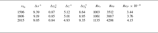
. The stretching function from Passiatore et al. (Reference Passiatore, Sciacovelli, Cinnella and Pascazio2021) is employed in the wall-normal direction to refine the near-wall region. Table 1 presents the different Reynolds numbers at three streamwise positions, along with the grid spacing in inner scales, denoted by the superscript
 $\boldsymbol{\cdot }^+$
. In the subsequent analysis of turbulent statistics, we will also use superscript
 $\boldsymbol{\cdot }^*$
to represent the semilocal scale. A seventh-order upwind scheme is used to discretise the convective terms, supplemented by a seventh-order weighted essentially non-oscillatory scheme activated in the regions of discontinuities, identified by a pressure-based shock sensor. An eighth-order centred difference scheme is employed for the viscous terms. The time stepping is performed using a third-order Runge–Kutta method, and the chemical reaction terms are stepped through the Strang splitting scheme. For a generic flow variable
 $\alpha$
, its fluctuation with respect to the Reynolds average
 $\overline {\alpha }$
is expressed as
 $\alpha '$
. The Favre average is denoted as
 $\widetilde {\alpha }$
, and the associated fluctuation is expressed as
 $\alpha ''$
.
Grid spacing and boundary-layer properties at three non-dimensional streamwise positions
 $x_{\delta _0}=x/\delta _0$
. Here
 $\Delta x^+$
,
 $\Delta y_w^+$
,
 $\Delta y_{\delta }^+$
and
 $\Delta z^+$
represent the grid sizes under the inner scale in their respective directions, with
 $\Delta y_w^+$
at the wall and
 $\Delta y_{\delta }^+$
at the boundary-layer edge. Here
 $\textit{Re}_{\tau }$
,
 $\textit{Re}_\theta$
and
 $\textit{Re}_{\delta ^*}$
correspond to the frictional, momentum and displacement Reynolds numbers, respectively.

3. The DNS results
Three-dimensional visualisation of the non-catalytic case. Vortex structures identified through the
 $\lambda _{c,i}$
-criterion, coloured with temperature field.

Two-dimensional spanwise instantaneous flow fields for temperature
 $T$
(a) and heat release rate
 $\dot {\omega }_h$
(b) under non-catalytic condition. A small streamwise portion is shown here to zoom in on the distribution of heat release rate close to the wall surface.

A three-dimensional visualisation of the turbulent flow field is provided in figure 1 for the non-catalytic case. The vortex structures are extracted using the
 $\lambda _{c,i}$
criterion, a vortex identification method suitable for compressible turbulence (Zhou et al. Reference Zhou, Adrian, Balachandar and Kendall1999; Kolár Reference Kolár2009; Lyu & Xu Reference Lyu and Xu2024). The vortices are coloured by temperature, showing a gradual transition from cold external fluid to heated fluid near the wall surface, and finally to the cold isothermal wall temperature prescribed in the computation set-up. The extracted turbulent flow corresponds to a region in the downstream portion of the computational domain where the boundary-layer flow is fully turbulent, characterised by elongated and tangled vortex tubes. These small-scale vortex structures are oriented randomly in all directions, indicating developed turbulence. Figure 2 provides a zoomed-in view of the instantaneous flow field at a spanwise section. While high temperatures near the wall surface are convected to the outer layer by turbulent mixing, the heat release distribution remains concentrated close to the wall surface. Strong heat absorption regions largely coincide with the high-temperature regions in the inner layer exceeding 4000 K.
We validate and examine the turbulent statistics, including velocity, temperature, species concentrations and chemical reaction rates. Three DNS runs are conducted in the present work: two chemically reacting runs with non-catalytic and catalytic conditions, and a supplementary non-reacting run. These three configurations enable examination of chemical reaction and wall catalysis effects on the turbulence. The corresponding settings are summarised in table 2. Comparison between reacting and non-reacting cases was only conducted under adiabatic wall conditions in previous literature (Passiatore et al. Reference Passiatore, Sciacovelli, Cinnella and Pascazio2021).
Chemical and catalytic settings of three DNS runs conducted in this work.

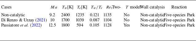
Our DNS validation involves comparing results from the non-catalytic case with similar flow configurations in Di Renzo & Urzay (Reference Di Renzo and Urzay2021) and Passiatore et al. (Reference Passiatore, Sciacovelli, Cinnella and Pascazio2022), focusing on spatially developing turbulent boundary layers with cold wall conditions. A comparison of computational parameters is provided in table 3. Wall-normal profiles of various statistics are extracted and compared at streamwise positions corresponding to a frictional Reynolds number
 $\textit{Re}_\tau$
exceeding 1100. We note that our inflow parameters originate from temporally evolving calculations in Duan & Martin (Reference Duan and Martin2011a
,Reference Duan and Martin
b
), differing from references in table 3. Comparison between temporally and spatially evolving cases has well-known issues, particularly in outer regions due to imposed transverse velocities (Li, Huang & Xu Reference Li, Huang and Xu2024), while the frictional Reynolds number also evolves streamwise in spatial settings, different from a temporal setting. Therefore, validation through comparison with spatially developing boundary layers under similar parameters is more appropriate, although magnitudes of turbulent statistics may vary slightly due to the specific parameter values employed.
Flow parameters in our simulated catalytic case and in reference cases from Di Renzo & Urzay (Reference Di Renzo and Urzay2021) and Passiatore et al. (Reference Passiatore, Sciacovelli, Cinnella and Pascazio2022). Here
 $T_w / T_r$
represents the wall/recovery temperature ratio. The recovery temperature is defined by
 $T_r=T_e (1+r((\gamma -1)/2)Ma^2)$
, where
 $\gamma$
is gas constant and
 $r$
is recovery coefficient (
 $r=0.89$
in our simulated non-catalytic case). Here
 $\textit{Re}_\tau$
represents the frictional Reynolds number of prescribed streamwise position where the wall-normal profiles are extracted. Two-
 $T$
model refers to the two-temperature model with translational–vibrational non-equilibrium, considered by Passiatore et al. (Reference Passiatore, Sciacovelli, Cinnella and Pascazio2022).

Non-dimensional mean chemical reaction rates of each species in semilocal scaling
 $y^{\ast }$
. (a) Comparison with Di Renzo & Urzay (Reference Di Renzo and Urzay2021). Close agreement achieved when the reference result is scaled by 1.35 due to lower temperature values (see temperature settings in table 3). Both calculations employ a single-temperature model. (b) Comparison between non-catalytic and catalytic cases.

Figure 3(a) presents wall-normal profiles of mean reaction rates
 $\bar {\dot {\omega }}_i$
for each species
 $i$
. The reaction rates are normalised by dynamic viscosity
 $\mu$
, density
 $\rho$
and wall shear stress
 $\tau _w$
. The obtained profiles closely match those in Di Renzo & Urzay (Reference Di Renzo and Urzay2021) when scaled by a factor of 1.35 for all five species. A magnitude difference is expected primarily due to the lower temperature setting in Di Renzo & Urzay (Reference Di Renzo and Urzay2021) (see table 3). The agreement in mean reaction rate profiles validates the calculation of chemical statistics in our data, which are very important for subsequent chemical closure model development. Figure 3(b) analyses wall catalysis effects on reaction rates. The supercatalytic condition reduces reaction rate magnitudes in the inner layer, particularly for NO and
 $\mathrm{O_2}$
, due to reaction suppression at the cold wall surface where gases remain recombined.
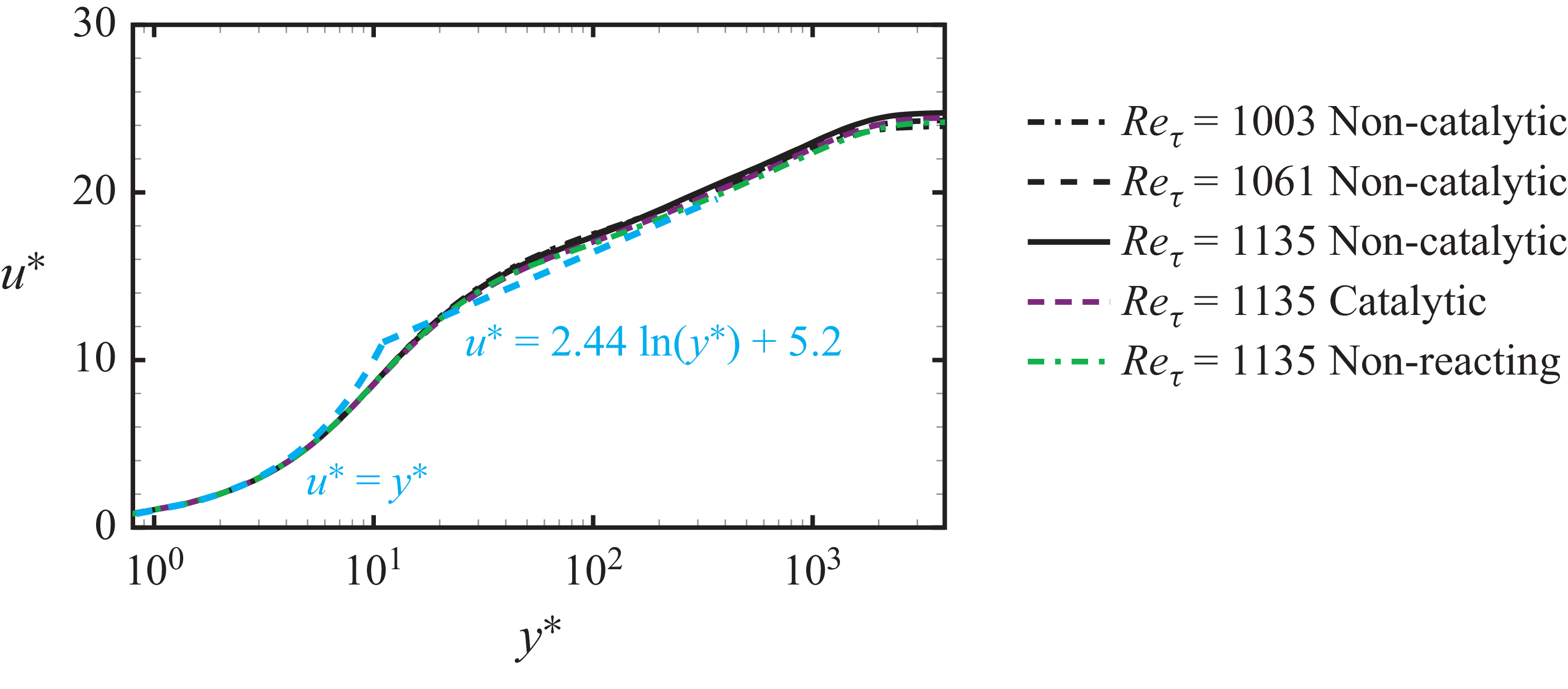
Mean velocity profile
 $u^{\ast }$
using the transformation of Griffin, Fu & Moin (Reference Griffin, Fu and Moin2021), at three streamwise positions of
 $\textit{Re}_\tau =1003,1061,1135$
for the non-catalytic case,
 $\textit{Re}_\tau =1135$
for the catalytic case and
 $\textit{Re}_\tau =1135$
for the non-reacting case. The linear and logarithmic laws are superposed.

Reynolds stresses normalised by the associated wall stresses. (a) Comparison with reference cases. (b) Comparison between different chemical and catalytic settings.

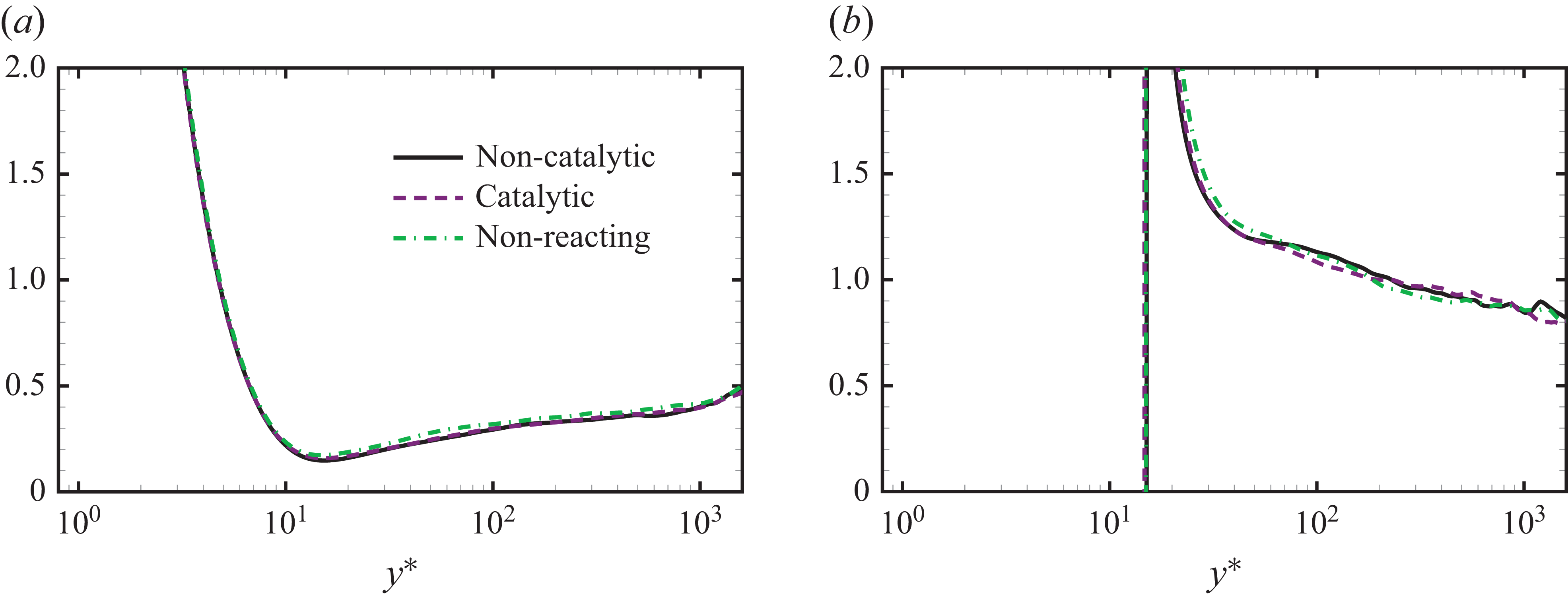
Figure 4 shows that the compressible transformation, proposed in Griffin et al. (Reference Griffin, Fu and Moin2021), can scale together velocity profiles across streamwise positions and different chemical/catalytic conditions. The scaled profiles follow the linear law
 $u^{\ast }=y^{\ast }$
and closely approach the logarithmic law
 $u^{\ast }=( {1}/{\kappa })\ln (y^{\ast })+B$
(
 $\kappa =0.41$
,
 $B=5.2$
). Figure 5(a) displays non-dimensional Reynolds stress profiles with reference data. The peak Reynolds normal stress (labelled with
 $uu$
) falls between reference values at similar
 $Ma$
and
 $\textit{Re}_\tau$
, while other components (labelled with
 $vv$
,
 $ww$
,
 $uv$
) closely match reference values. Figure 5(b) reveals slight reductions of Reynolds normal stress magnitudes by chemical reactions, whereas differences in catalytic conditions leads to little difference. The slight decrease of normal stresses by chemical reaction was also observed in Passiatore et al. (Reference Passiatore, Sciacovelli, Cinnella and Pascazio2021) in an adiabatic setting, which was attributed to the drained turbulent energy by chemical heat absorption.
First- and second-order temperature statistics between different chemical and catalytic settings: (a) mean temperature; (b) root-mean-square of temperature.

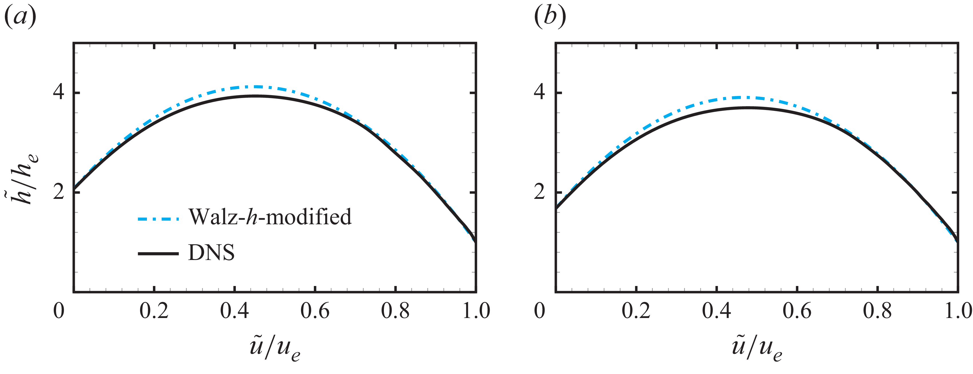
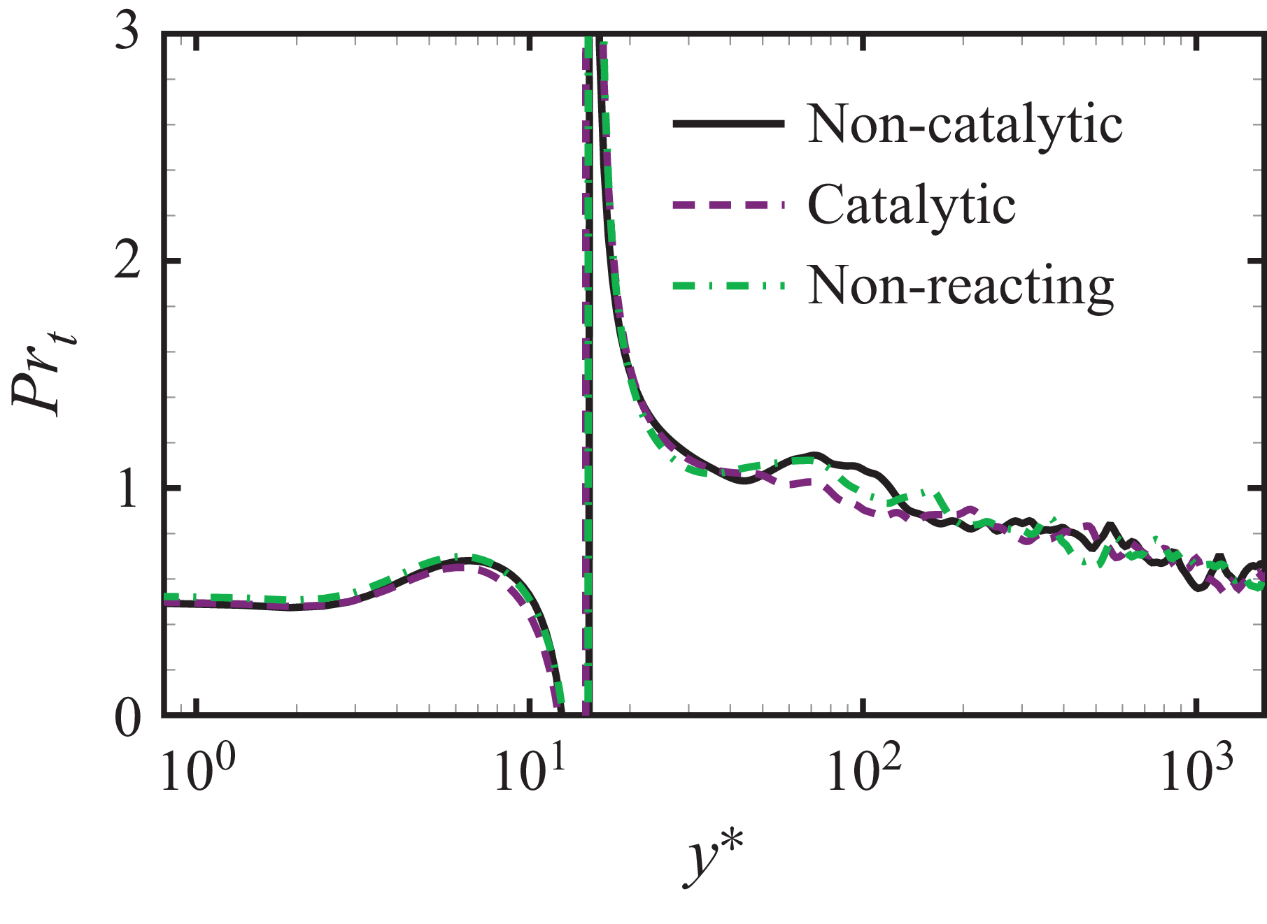
First- and second-order temperature statistics are analysed in figure 6. The maximum mean temperature in our calculations reaches approximately 4500 K. Compared with the non-reacting case, the chemical heat absorption reduces the maximum mean temperature of around 200 K. No distinguishable difference in mean temperature is observed between different catalytic conditions. The temperature fluctuation distributions exhibit two distinct peaks, and the endothermic reaction is shown to have a significant effect on reducing temperature fluctuations in both inner and outer layers. The non-catalytic condition produces a stronger reduction in temperature fluctuations, consistent with higher chemical reaction rates. These reaction effects on temperature statistics agree with those reported in Passiatore et al. (Reference Passiatore, Sciacovelli, Cinnella and Pascazio2021). We have further examined various correlations of temperature and velocity statistics, including Walz’s scaling, strong Reynolds analogies and turbulent Prandtl numbers. Overall, these temperature–velocity correlations exhibit behaviours similar to those observed in non-reacting flows with cold walls (except that an enthalpy-based formulation is required for Walz’s scaling), indicating that chemical reactions do not substantially alter the relationships between temperature and velocity. The associated results are provided in Appendix A.
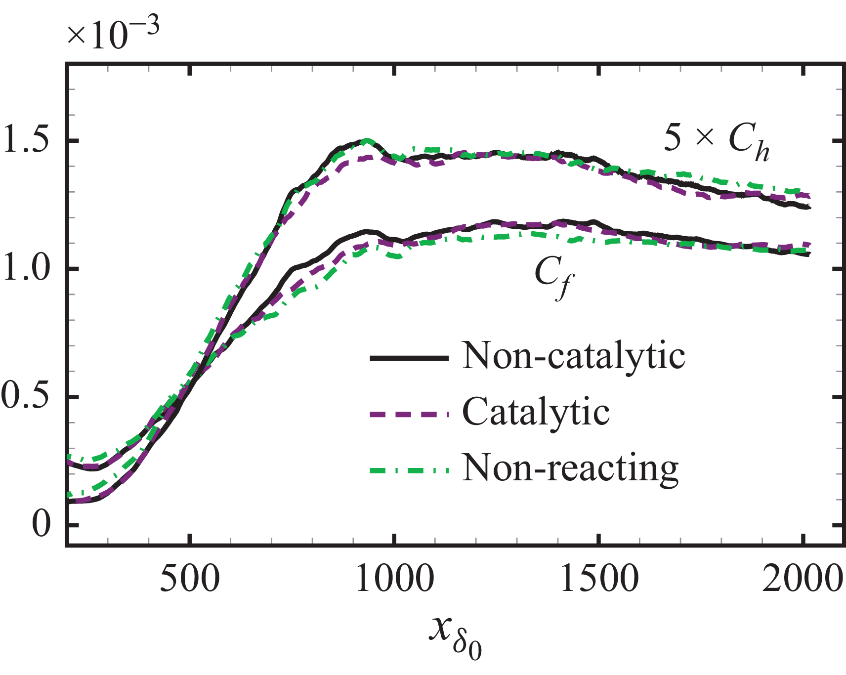
Skin friction coefficient
 $C_{\!f}$
and wall heat flux coefficient
 $C_h$
scaled by five (
 $5\times C_h$
) at different streamwise positions
 $x_{\delta _0}$
.

Mean molar fraction of each species under non-catalytic and catalytic conditions.

The influence of chemistry and catalysis on wall quantities is further analysed in figure 7. Streamwise evolutions of the non-dimensional skin friction coefficient
 $C_{\!f}$
and heat flux coefficient
 $C_h$
are presented. The coefficients are defined by
 $C_{\!f}=\tau _w / (0.5 \rho _e U_e^2)$
and
 $C_h=q_w / (\rho _e U_e^3)$
, respectively, where
 $q_w$
denotes the wall heat flux. The finite-rate chemical reactions have a weakly distinguishable effect in the transition region, linked to the increase of
 $C_{\!f}$
and
 $C_h$
. Farther downstream, the wall heat flux coefficient
 $C_h$
show little difference between the reacting and non-reacting cases, whereas the maximum difference in
 $C_{\!f}$
between the non-catalytic and non-reacting cases is capped at below 6.5 %, with little difference after
 $x_{\delta _0}=1600$
. The streamwise evolution of
 $C_{\!f}$
is controlled by the wall shear strain
 ${({\rm d}U/{\rm d}y)}_w$
and the wall dynamical viscosity
 $\mu _w$
. The latter depends only on the species mass fraction at the wall surface because the wall temperature is fixed. Further evaluations show that the maximum difference in
 $\mu _w$
at different streamwise positions among the three simulated cases is lower than 1 %, while the streamwise evolution of
 ${({\rm d}U/{\rm d}y)}_w$
among different cases closely resembles that of
 $C_{\!f}$
. Therefore, the slight differences observed in
 $C_{\!f}$
can be primarily attributed to the modulation of wall shear strain by the finite-rate reaction. A similar influence on
 $C_{\!f}$
was observed in Passiatore et al. (Reference Passiatore, Sciacovelli, Cinnella and Pascazio2021), where the skin friction of reacting and non-reacting cases does not align in the transition region, but coincides with each other in the developed turbulent region, despite the important reaction rate at the hot wall surface.
The molar fraction for
 $i$
th species, denoted as
 $X_i$
, is expressed as
 $X_i=Y_i/M_i/\sum _j(Y_j/M_j)$
, where
 $M_i$
is the molar mass of
 $i$
th species. Wall-normal profiles of the mean molar fraction for each species are presented in figure 8 under both non-catalytic and catalytic conditions. For a non-catalytic surface, the dissociation of
 $\mathrm{O_2}$
and
 $\mathrm{N_2}$
, together with generation of
 $\mathrm{O}$
and
 $\mathrm{NO}$
, leads to nearly monotonous species distributions from the wall surface to the outer layer, except for
 $N$
, which peaks in the inner region due to a non-zero consumption rate at the surface (see figure 10
d in the following). For the catalytic case under the cold wall condition, little chemical reaction takes place at the wall surface. Therefore, the wall-normal profile of reaction rates peaks in the inner layer with overall reduced rate magnitudes.
4. Turbulent chemistry closure
4.1. Analysis of turbulence–chemistry interaction in a PDF framework
We consider the closure of chemical source terms, including the production rate
 $\dot {\omega }_i$
and the associated chemical heat release rate
 $\dot {\omega }_h$
. In general, the contribution to mean chemical source terms from temperature and species compositions is analysed from a statistical perspective using PDF formulations. These formulations were employed in Wang & Xu (Reference Wang and Xu2024) to analyse the turbulence–chemistry interaction in a boundary-layer with combustion. The analysis and model development in this section are based on DNS data simulated with non-catalytic conditions. Highly similar results are found for catalytic condition, provided in Appendix B.
We consider the sample space of temperature and species mass fractions associated with the chemical source terms, denoted as
 $\hat {T}$
and
 $\hat {\boldsymbol{Y}}$
, respectively. An arbitrary ensemble-averaged chemical source term, such as the turbulent chemical heat release rate
 $\bar {\dot {\omega }}_h$
, can be obtained by integrating chemical heat release rate with the corresponding JPDF of temperature and species mass fractions, denoted as
 $P(\hat {T},\hat {\boldsymbol{Y}})$
. Thus, the expression for the turbulent chemical heat release rate is given by
 \begin{equation} \overline {\dot {\omega }}_h (T,\boldsymbol{Y}) = \int \dot {\omega }_h(\hat {T},\hat {\boldsymbol{Y}} ) \boldsymbol{P}(\hat {T},\hat {\boldsymbol{Y}} ) {\rm d} \hat {T} {\rm d} \hat {\boldsymbol{Y}}. \end{equation}
Whereas the form of
 $\boldsymbol{P}(\hat {T},\hat {\boldsymbol{Y}} )$
can be perfectly known within a set of DNS data, the aim of closure problem is to model this JPDF. To offer a direct perspective, the laminar closure, or the non-modelling of heat release rate can be expressed as
 \begin{equation} \dot {\omega }_h (\overline {T},\overline {\boldsymbol{Y}}) = \int \dot {\omega }_h(\hat {T},\hat {\boldsymbol{Y}} ) \delta (\hat {T}-\bar {T}) \delta (\hat {\boldsymbol{Y}}-\bar {\boldsymbol{Y}}) {\rm d} \hat {T} {\rm d} \hat {\boldsymbol{Y}}, \end{equation}
where
 $\delta (\hat {T}-\bar {T})$
and
 $\delta (\hat {\boldsymbol{Y}}-\bar {\boldsymbol{Y}})$
are delta functions to ensure
 $\hat {T}$
and
 $\hat {\boldsymbol{Y}}$
can only take their mean values. The wall-normal profiles of turbulent and laminar heat release rates are shown in figure 9, with negative values signifying an endothermic reaction. The discrepancy at the peak position represents 25 % of the peak value of the turbulent heat release rate.
Diagnostic heat release rates defined in (4.3) and (4.4):
 $\breve {\dot {\omega }}_h|_{\bar {Y}_{{\rm O_2}}}$
,
 $\breve {\dot {\omega }}_h|_{\bar {Y}_{{\rm O}}}$
,
 $\breve {\dot {\omega }}_h|_{\bar {Y}_{{\rm NO}}}$
,
 ${{\varepsilon }^{*}}={\varepsilon }/{{{\varepsilon }_{\textit{max}}}}$
,
 $\breve {\dot {\omega }}_h|_{\bar {Y}_{{\rm N}_2}}$
(a–e) and
 $\breve {\dot {\omega }}_h|_{\bar {T}}$
( f). The same profiles of turbulent and laminar heat release rates,
 $\overline {\dot {\omega }}_h (T,\boldsymbol{Y})$
and
 $\dot {\omega }_h (\overline {T},\overline {\boldsymbol{Y}})$
, are provided in each panel. Results are obtained from data under non-catalytic conditions at
 $\textit{Re}_\tau =1135$
.

We then investigate which variables’ probability distributions are not being modelled, thereby resulting in this discrepancy. For this analysis, we assume that only the mean value of a species mass fraction,
 $\bar {Y}_i$
, is known, while we have perfect knowledge of the JPDF of the other variables from DNS data. In this setting, a diagnostic heat release rate related to the non-modelling of
 $\bar {Y}_i$
, denoted as
 $\breve {\dot {\omega }}_h|_{\bar {Y}_i}$
, can be defined as
 \begin{align} \breve {\dot {\omega }}_h|_{\bar {Y}_i} &=\overline {\dot {\omega }}_h (T,Y_1,\ldots ,\bar {Y}_{i},\ldots ,Y_N) \nonumber \\&=\int \dot {\omega }_h(\hat {T},\hat {\boldsymbol{Y}} ) \boldsymbol{P}(\hat {T},\hat {Y}_1,\ldots ,\hat {Y}_{i-1},\hat {Y}_{i+1},\ldots ,\hat {Y}_{N})\delta (\hat {Y}_i-\bar {Y}_i) {\rm d} \hat {T} {\rm d} \hat {\boldsymbol{Y}}. \end{align}
Accordingly, a diagnostic heat release rate related to the non-modelling of temperature
 $\bar {T}$
can be written as
 \begin{equation} \breve {\dot {\omega }}_h|_{\bar {T}}=\overline {\dot {\omega }}_h (\bar {T},\boldsymbol{Y})=\int \dot {\omega }_h(\hat {T},\hat {\boldsymbol{Y}} ) \boldsymbol{P}(\hat {\boldsymbol{Y}})\delta (\hat {T}-\bar {T}) {\rm d} \hat {T} {\rm d} \hat {\boldsymbol{Y}}. \end{equation}
The wall-normal profiles of
 $\breve {\dot {\omega }}_h|_{\bar {Y}_i}$
and
 $\breve {\dot {\omega }}_h|_{\bar {T}}$
are shown in figure 9, superposed by the turbulent heat release rate
 $\overline {\dot {\omega }}_h (T,\boldsymbol{Y})$
and that with laminar closure
 $\dot {\omega }_h (\overline {T},\overline {\boldsymbol{Y}})$
. All profiles of
 $\breve {\dot {\omega }}_h|_{\bar {Y}_i}$
closely align with the turbulent heat release rate, indicating that the calculation of turbulent heat release rate is minimally influenced by the absence of knowledge regarding higher moments of species mass fractions. In contrast, the modelling of temperature fluctuation is crucial for closing the turbulent heat release rate: the profile of
 $\breve {\dot {\omega }}_h|_{\bar {T}}$
considerably deviates from the turbulent heat release rate, and is observed to be closely aligned with the laminar one. This finding clearly suggests that the non-modelling of temperature fluctuation is the primary cause of the substantial discrepancy between turbulent and laminar heat release rates.
Chemical source terms modelled with
 $\boldsymbol{P}(\hat {T})$
from DNS, as defined in (4.5) and (4.6):
 $\tilde {\dot {\omega }}_{{\rm O_2}}$
,
 $\tilde {\dot {\omega }}_{\mathrm{O}}$
,
 $\tilde {\dot {\omega }}_{\mathrm{NO}}$
,
 $\tilde {\dot {\omega }}_{\mathrm{N}}$
,
 $\tilde {\dot {\omega }}_{{\rm N_2}}$
(a–e) and
 $\tilde {\dot {\omega }}_h$
( f) . The associated turbulent source terms
 $\overline {\dot {\omega }}_i (T,\boldsymbol{Y})$
,
 $\overline {\dot {\omega }}_h (T,\boldsymbol{Y})$
and the laminar source terms
 $\dot {\omega }_i (\overline {T},\overline {\boldsymbol{Y}})$
,
 $\dot {\omega }_h (\overline {T},\overline {\boldsymbol{Y}})$
are superposed. Non-catalytic condition at
 $\textit{Re}_\tau =1135$
with rate values in SI units.

The analysis above indicates a closure strategy that involves modelling only the temperature distribution, utilising the straightforward knowledge of mean species concentrations. In this context, the modelled productions rates and heat release rates, represented by
 $\tilde {\dot {\omega }}_i$
and
 $\tilde {\dot {\omega }}_h$
, respectively, are proposed as
 \begin{align} \tilde {\dot {\omega }}_i=\overline {\dot {\omega }}_i (T,\bar {\boldsymbol{Y}})=\int \dot {\omega }_i(\hat {T},\hat {\boldsymbol{Y}} ) \boldsymbol{P}(\hat {T})\delta (\hat {\boldsymbol{Y}}-\bar {\boldsymbol{Y}}) {\rm d} \hat {T} {\rm d} \hat {\boldsymbol{Y}}, \end{align}
 \begin{align} \tilde {\dot {\omega }}_h=\overline {\dot {\omega }}_h (T,\bar {\boldsymbol{Y}})=\int \dot {\omega }_h(\hat {T},\hat {\boldsymbol{Y}} ) \boldsymbol{P}(\hat {T})\delta (\hat {\boldsymbol{Y}}-\bar {\boldsymbol{Y}}) {\rm d}\hat {T} {\rm d} \hat {\boldsymbol{Y}}. \end{align}
To assess the validity of this closure strategy, we start with temperature distribution
 $\boldsymbol{P}(\hat {T})$
that can be perfectly known from DNS data. Figure 10 shows
 $\tilde {\dot {\omega }}_i$
and
 $\tilde {\dot {\omega }}_h$
, using
 $\boldsymbol{P}(\hat {T})$
from DNS. In each panel, the modelled chemical source terms approximately match the turbulent chemical source terms, with the exception of the production rate of atomic nitrogen
 $\mathrm{N}$
. Given that the mass fraction of N is around three orders of magnitudes smaller than that of the other species within the simulated temperature range (Duan & Martin Reference Duan and Martin2011a
; Di Renzo & Urzay Reference Di Renzo and Urzay2021) and the modelled chemical heat release is well aligned with the turbulent one, we infer that this discrepancy related to N has a negligible impact on the turbulent heat release rate, but the analysis in § 5 also shows that it may influence the robustness of wall models using the developed chemical closure. There is also a slight degree of mismatch in the outer region for modelling the rate values of
 $\mathrm{O}_2$
and O. Nevertheless, the discrepancy in the inner region, which is considered more crucial for the near-wall statistics, has been markedly reduced. The assessment shows that the involved reaction, within the explored flow parameter ranges, is primarily controlled by the temperature. This finding is consistent with the mechanism of pollutant formation, such as
 $\mathrm{NO}_x$
in burnt gases (see page 235 of Poinsot & Veynante (Reference Poinsot and Veynante2005)). Consequently, an accurate model of the temperature distribution would effectively close the turbulent chemical source terms.
4.2. Modelling the temperature probability distribution
The assessment previously discussed relies on the precise distribution of temperature obtained from DNS, which is not accessible in RANS simulations. In practice, we use the first- and second-order moments of temperature to model the temperature distribution
 $\boldsymbol{P}(\hat {T})$
, by assuming different forms of PDFs. The required temperature variance can be modelled through an augmented transport equation similar to the kinetic energy transport equation, which has been widely used for RANS modelling of turbulent combustion (Spalding Reference Spalding1971; Lockwood & Naguib Reference Lockwood and Naguib1975; Baurle & Girimaji Reference Baurle and Girimaji2003; Poinsot & Veynante Reference Poinsot and Veynante2005). Alternatively, the specific boundary-layer configuration offers the possibility to model temperature fluctuations through velocity analogy (Zhang et al. Reference Zhang, Bi, Hussain, Li and She2012; Huang et al. Reference Huang, Su, Guo, Yuan, Xiong and Zhou2025) or relevant scaling laws (Martin & Candler Reference Martin and Candler2001). Therefore, we assume that the first- and second-order moments of temperature are known quantities, and their exact values will be extracted from DNS in subsequent modelling processes.
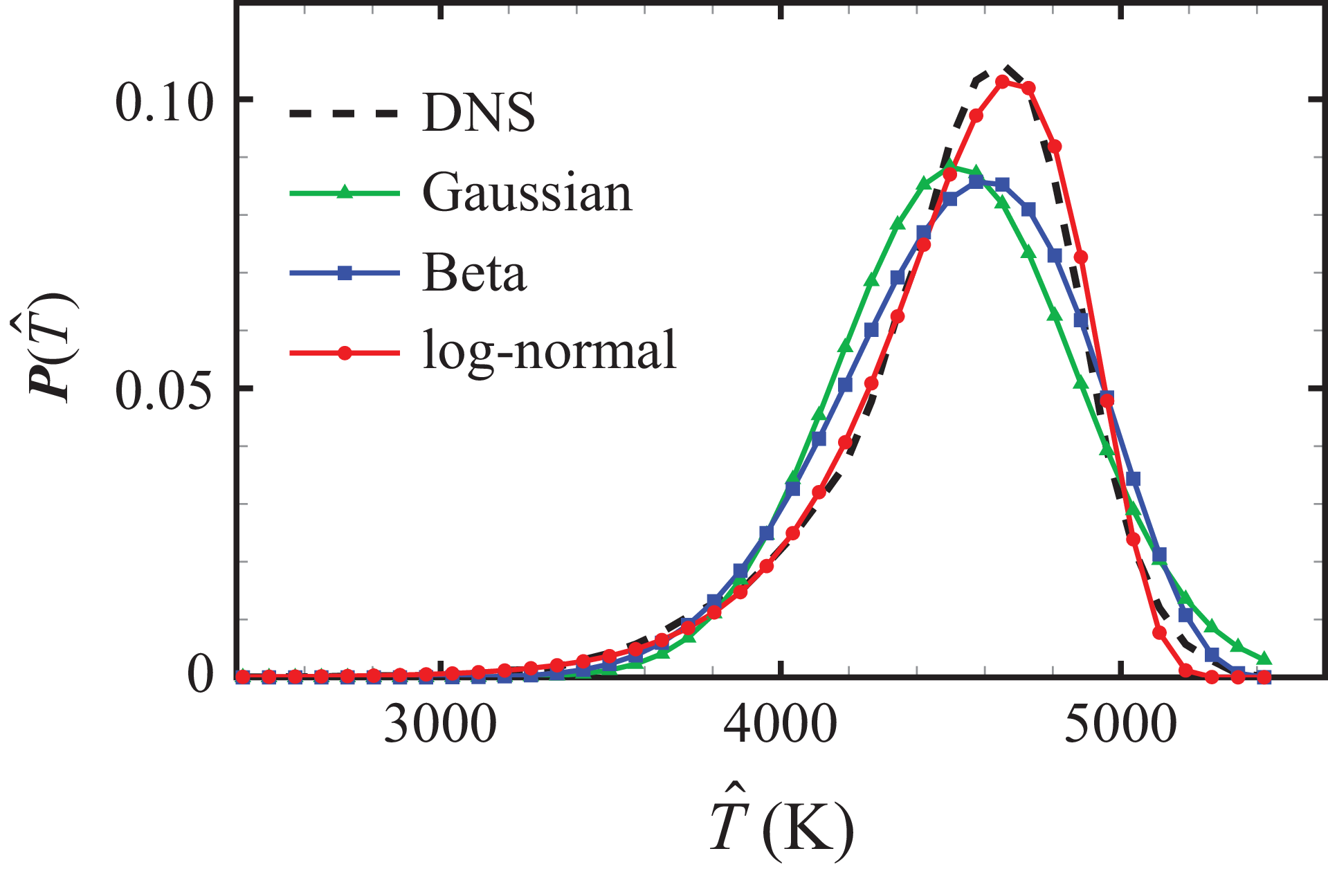
Figure 11 displays the temperature PDF at the position of the peak reaction rate
 $y^\ast =11.1$
. The PDF is observed to be asymmetric, with a long tail stretching towards the wall temperature value,
 $T_w=2400$
K. This temperature PDF allows to comprehensively explain the discrepancy between turbulent and laminar reaction rates shown in figure 9: because the temperature distribution is skewed negatively, considering only the mean temperature reduces the impact of high temperatures, thereby leading to lower estimated rate values.
Temperature PDF at
 $y^{\ast }=11.1$
. The PDF obtained from DNS is depicted with a dashed line in black. Model PDFs using Gaussian, Beta and log-normal distributions are overlaid. Non-catalytic condition at
 $\textit{Re}_\tau =1135$
.

The observed skewed distributions of scalar variables have been identified both experimentally and numerically in incompressible turbulent channel flows and boundary-layer flows over several decades (Antonia, Krishnamoorthy & Fulachier Reference Antonia, Krishnamoorthy and Fulachier1988; Nagano & Tagawa Reference Nagano and Tagawa1988; Li et al. Reference Li, Schlatter, Brandt and Henningson2009). However, the temperature PDF in the near-wall region of compressible boundary-layer flows has been little explored. In turbulent flames, temperature PDFs are commonly modelled using either Gaussian or Beta distributions (Poinsot & Veynante Reference Poinsot and Veynante2005). The Gaussian distribution is symmetric and requires only the mean value
 $\bar {T}$
and the variance
 $T'^2$
as parameters. The Beta distribution, defined on a bounded interval, incorporates four parameters:
 $\bar {T}$
,
 $T'^2$
and the interval limits, denoted as
 $T_{\textit{min}}$
and
 $T_{\textit{max}}$
, respectively. In a coaxial supersonic burner (Baurle & Girimaji Reference Baurle and Girimaji2003), the limits were estimated as
 $T_{\textit{min}}=\bar {T}-3T'$
and
 $T_{\textit{max}}=\bar {T}+3T'$
, but this estimation leads to a symmetric distribution.
For the present study, we evaluate both Gaussian and Beta distributions to fit the temperature PDF. For the Beta distribution parameters, we retain
 $T_{\textit{max}}=\bar {T}+3T'$
but propose setting the minimum limit as the wall temperature
 $T_{\textit{min}}=T_w$
to produce an asymmetric distribution. However, as illustrated in figure 11, both distributions fail to accurately reproduce the temperature PDF obtained from DNS, with the modelled Beta distribution proving insufficiently skewed.
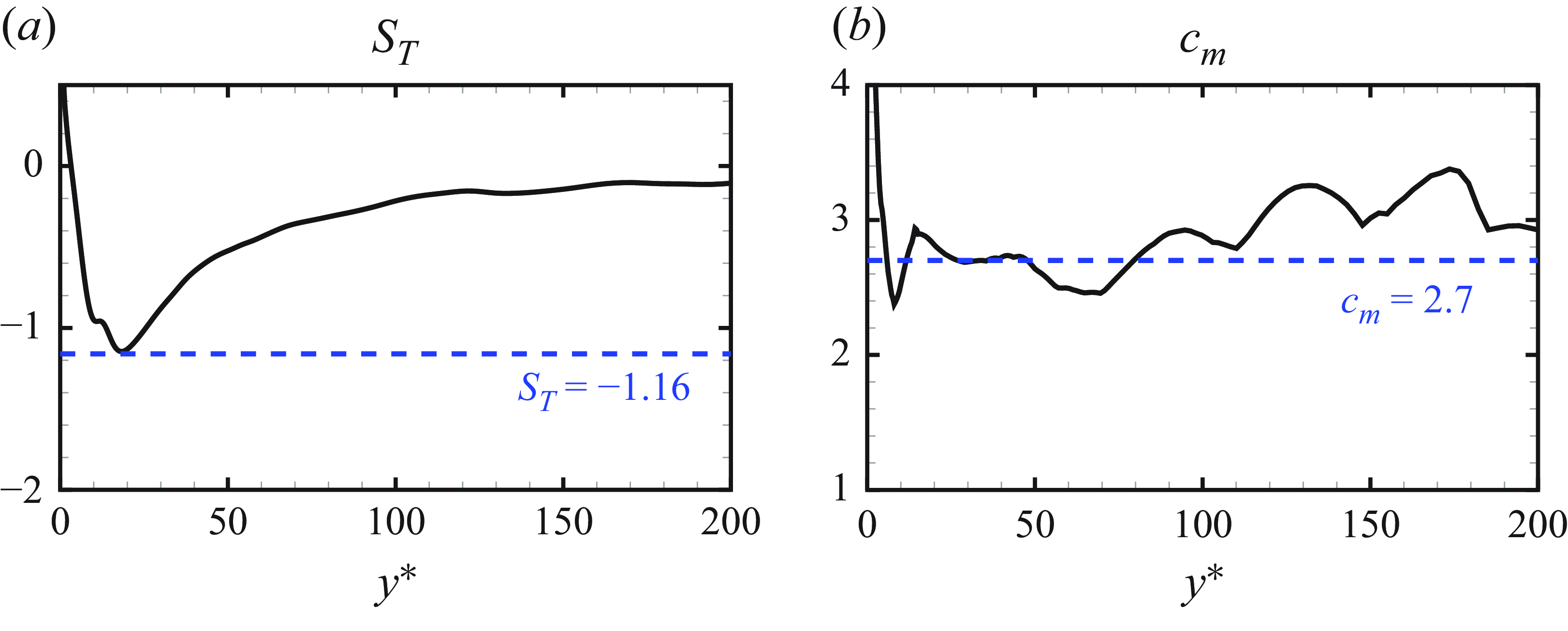
(a) Wall-normal profiles of temperature skewness
 $S_T$
, evaluated from DNS. Here
 $S_T=-1.16$
is represented by the dashed line in blue. (b) Wall-normal profiles of log-normal model constant
 $c_m$
, evaluated from DNS. Here
 $c_m=2.7$
is represented by the dashed line in blue. Non-catalytic condition at
 $\textit{Re}_\tau =1135$
.

We further consider the log-normal distribution, which is inherently asymmetric. The PDF for a random variable
 $\phi$
in the log-normal distribution is expressed as
 \begin{equation} \boldsymbol{P}(\phi )=\frac {1}{\phi \sigma \sqrt {2 \pi }}\exp\! \left ( -\frac {(\ln \phi - \mu )^2}{2 \sigma ^2} \right )\!, \end{equation}
where
 $\mu$
and
 $\sigma$
are the location and scale parameters, respectively. Given that
 $\boldsymbol{P}(\phi )$
is defined for positive values, corresponding to a semibounded region, an additional bounding parameter
 $T_{\textit{max}}$
is required. Since the temperature PDF is skewed towards the negative side, the random variable in (4.7) should be taken as
 $\phi =T_{\textit{max}} -T$
. The distribution parameters
 $\mu$
and
 $\sigma$
are supposed to be identified by the method of moments using the mean and variance of random variable,
 \begin{equation} \mu =\log \big ( \bar {\phi }/\sqrt {1+\phi '^2/\bar {\phi }^2} \big ), \qquad \sigma =\sqrt {\log \big ( 1+\phi '^2/\bar {\phi }^2 \big ) }. \end{equation}
Additionally, we assume
 \begin{equation} T_{\textit{max}}=\bar {T}+c_m T', \end{equation}
where
 $c_m$
is a model constant. This assumption draws a direct link between
 $c_m$
and the skewness of temperature distribution. The skewness of random variable
 $\phi$
satisfying a log-normal distribution can be calculated by
 \begin{equation} S_{\phi }=\big (\exp (\sigma ^2)+2 \big ) \sqrt {\exp (\sigma ^2)-1}, \end{equation}
and the temperature skewness
 $S_T$
is given by
 $S_T=-S_{\phi }$
. Combining (4.8), (4.9) and (4.10), the expression of
 $S_T$
can be expressed as
 \begin{equation} S_T=-\big ( 3+ 1/c_m^2 \big ) /c_m. \end{equation}
We evaluate
 $c_m=(T_{\textit{max}}-\bar {T})/T'$
using DNS data at different wall-normal positions, as shown in figure 12(b). We adopt a constant value of
 $c_m=2.7$
as an estimate. The modelled temperature PDF with the log-normal distribution is observed to closely match the exact PDF of temperature at the peak position of the reaction rate, as illustrated in figure 11. An important reason of this good match is that the skewness of temperature can be well represented: inserting
 $c_m=2.7$
into (4.11) leads to a temperature skewness
 $S_T=-1.16$
. Figure 12(a) displays the wall-normal profile of
 $S_T$
from DNS, superposed by a dashed line representing
 $S_T=-1.16$
. It is observed that the skewness value evaluated from DNS is around
 $-1$
in the peak rate region, which allows a good modelling of temperature distribution. The skewness value deviates from
 $-1$
at other wall-normal positions, and the impact of this discrepancy on the computed rate values is examined in the subsequent analysis.
4.3. Model assessment
Chemical source terms modelled with
 $\boldsymbol{P}(\hat {T})$
of the log-normal distribution, as defined in (4.5), (4.6) and (4.7):
 $\tilde {\dot {\omega }}_{{\rm O_2}}$
,
 $\tilde {\dot {\omega }}_{\mathrm{O}}$
,
 $\tilde {\dot {\omega }}_{\mathrm{NO}}$
,
 $\tilde {\dot {\omega }}_{\mathrm{N}}$
,
 $\tilde {\dot {\omega }}_{{\rm N_2}}$
(a–e) and
 $\tilde {\dot {\omega }}_h$
( f). The associated turbulent source terms and the laminar source terms are superposed in each panel. Non-catalytic condition at
 $\textit{Re}_\tau =1135$
with rate values in SI units.

Figure 13 presents the wall-normal profiles of the modelled turbulent chemical source terms,
 $\tilde {\dot {\omega }}_i$
and
 $\tilde {\dot {\omega }}_h$
, calculated using (4.5) and (4.6) with
 $\boldsymbol{P}(\hat {T})$
modelled by the log-normal distribution. The modelled rate profiles are in good agreement with the turbulent ones, achieving a level of consistency comparable to that of the profiles using the precise temperature PDF from DNS data in figure 10 (green dotted). The discrepancy of temperature skewness
 $S_T$
at certain wall-normal positions, as shown in figure 12(a), does not notably compromise the agreement of modelled rate values against the turbulent ones.
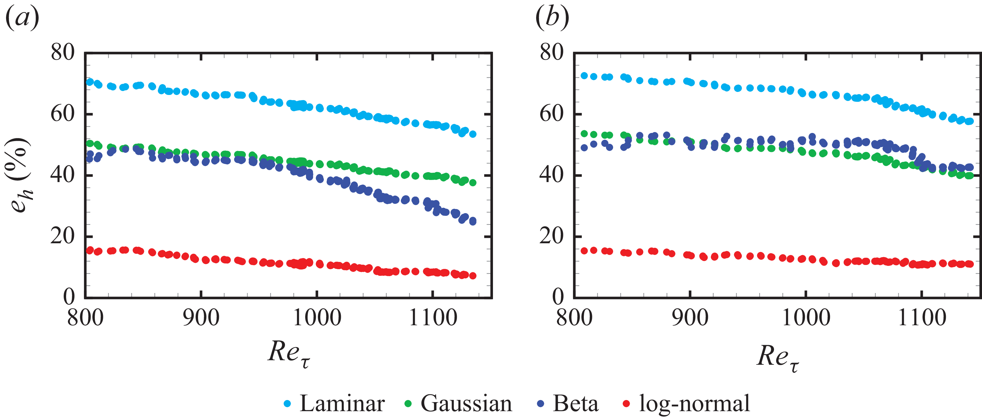
We further evaluate the closure results at various streamwise positions. To quantify the error of the closure with respect to the turbulent heat release rate
 $\overline {\dot {\omega }}_{h}$
across the entire boundary layer, we define an error metric
 $e_{h}$
as follows:
 \begin{equation} e_{h}=\dfrac {\int _{0}^{\delta }\big |\tilde {\dot {\omega }}_{h}-\overline {\dot {\omega }}_{h}\big |{\rm d}y}{\int _{0}^{\delta }\big |\overline {\dot {\omega }}_{h}\big | {\rm d}y}, \end{equation}
where the modelled chemical heat release rates,
 $\tilde {\dot {\omega }}_{h}$
, are computed with laminar closure, or with
 $\boldsymbol{P}(\hat {T})$
using Gaussian, Beta and log-normal distributions. Figure 14 displays the error metric
 $e_{h}$
at different streamwise positions, labelled by the frictional Reynolds number
 $\textit{Re}_\tau$
. Results under both non-catalytic and catalytic conditions are presented. The use of the log-normal distribution significantly decreases
 $e_{h}$
compared with the laminar closure and also yields better results than Gaussian and Beta distributions. The error metric
 $e_{h}$
of all closure models shows a slightly decreasing trend with
 $\textit{Re}_\tau$
, which can be attributed to the overshoot of fluctuation magnitudes associated with the flow transition in the upstream positions (Di Renzo & Urzay Reference Di Renzo and Urzay2021; Passiatore et al. Reference Passiatore, Sciacovelli, Cinnella and Pascazio2022). Specifically at
 $\textit{Re}_\tau =1135$
under non-catalytic conditions,
 $e_{h}$
is reduced to 7 % compared with 54 % using the laminar closure.
Error metric
 $e_{h}$
, defined by (4.12), evaluated at different streamwise positions and plotted against the frictional Reynolds number
 $\textit{Re}_{\tau }$
. Results are presented for closure with
 $\boldsymbol{P}(\hat {T})$
of Gaussian, Beta and log-normal distributions, along with the laminar closure: (a) non-catalytic condition; (b) catalytic condition.

4.4. Study of model parameter
 $S_T$
: dependence and sensitivity

The inputs of present model consist of temperature and species mean values, as well as temperature fluctuations, which are assumed to be accessible in RANS calculations. By contrast, the single model constant that still needs to be prescribed is the temperature skewness
 $S_T$
, which was calibrated from DNS in the model development process. In this section, two separate studies are conducted on this model parameter.
Wall-normal profiles of mean temperature (a) and temperature skewness (b) evaluated from compressible channel flow databases at different Mach numbers in Yu, Xu & Pirozzoli (Reference Yu, Xu and Pirozzoli2019). See table 4 for case parameters.

The first study evaluates temperature skewness at different Mach numbers
 $Ma$
and wall temperatures
 $T_w$
, using DNS databases of compressible turbulent channel flows simulated with streamwise periodic conditions without chemical reactions. This evaluation aims to examine the dependence of
 $S_T$
, thereby providing guidelines for selecting this value under different flow conditions. The dependence of
 $S_T$
on Mach number
 $Ma$
is analysed using the database of Yu et al. (Reference Yu, Xu and Pirozzoli2019), which contains channel flows at reference Mach numbers
 $M_0$
ranging from 0.8 to 8.0 under isothermal hot wall conditions
 $T_w / T_r =1$
. The corresponding Mach numbers and frictional Reynolds numbers for each considered case are listed in table 4. Figure 15(a) presents the non-dimensional mean temperature profiles, where the centreline temperature is normalised to unity in each case. The wall temperature increases with Mach number due to the approximate adiabatic condition associated with the recovery temperature
 $T_r$
. As shown in figure 15(b), the temperature skewness exhibits little variation across Mach numbers and consistently peaks at
 $y^*=10$
. These results indicate that the temperature skewness depends only weakly on the Mach number.
Flow parameters of the compressible channel flow database at different Mach numbers in Yu et al. (Reference Yu, Xu and Pirozzoli2019). Here
 $M_0$
is the reference Mach number of inflow fluid stream. The wall/recovery temperature ratio,
 $T_w/T_r$
, is set to be unity in all cases, representing an approximate adiabatic condition estimated by recovery temperature.

Wall-normal profiles of mean temperature (a) and temperature skewness (b) evaluated from compressible channel flow databases at different wall/recovery temperature ratios
 $T_w/T_r$
in Yu & Xu (Reference Yu and Xu2021). See table 5 for case parameters.

The dependence of
 $S_T$
on wall temperature
 $T_w$
is further investigated using data from Yu & Xu (Reference Yu and Xu2021). The database comprises three simulation sets with
 $T_w / T_r$
ranging from 0.2 to 1.0 at comparable frictional Reynolds numbers and centreline Mach numbers
 $M_c$
, as listed in table 5. Figure 16 demonstrates that
 $S_T$
varies with the wall temperature, although it maintains negative peak values in the near-wall region across all cases. Colder wall temperatures result in reduced peak magnitudes and shift the peak position farther from the wall. This behaviour of skewness can be physically interpreted: under hot-wall conditions, turbulent convection transports both hot fluid from the near-wall region and cold fluid from the outer layer to the
 $y^*=10$
region, generating skewed temperature fluctuations. In contrast, cold-wall conditions (e.g. case CW02 in figure 16) involve cold fluid transported from both the wall-adjacent and outer regions, producing smaller skewness values compared with hot-wall cases.
Flow parameters of the compressible channel flow database at different wall/recovery temperature ratios
 $T_w/T_r$
in Yu & Xu (Reference Yu and Xu2021). Here
 $M_c$
is the Mach number at the centreline of planer channel.

The temperature ratio
 $T_w/T_r=0.2$
in CW02 is relatively close to the prescribed ratio
 $T_w/T_r=0.121$
in our catalytic case, as listed previously in table 3. Accordingly, similar peak characteristics are observed:
 $S_T=-1.06$
at
 $y^*=16$
for CW02 (periodic channel) and
 $S_T=-1.16$
at
 $y^*=18$
in our non-catalytic boundary layer. These comparable values across different Reynolds numbers may relate to recent findings of universal velocity PDF scaling in the logarithmic region of wall-bounded turbulence (Ge, Yang & Marusic Reference Ge, Yang and Marusic2019).
In the second study, we directly assess the sensitivity of closure results to different values of
 $S_T$
, by re-evaluating the results in figures 13( f) and 14(a). Such a sensitivity analysis may be particularly useful, since the present configuration closely resembles previous cold-wall DNS calculations, which are more representative of practical flight conditions that would eventually be simulated using RANS equations. Two values,
 $S_T=-0.8$
and
 $S_T=-2$
, are considered, covering the range of
 $S_T$
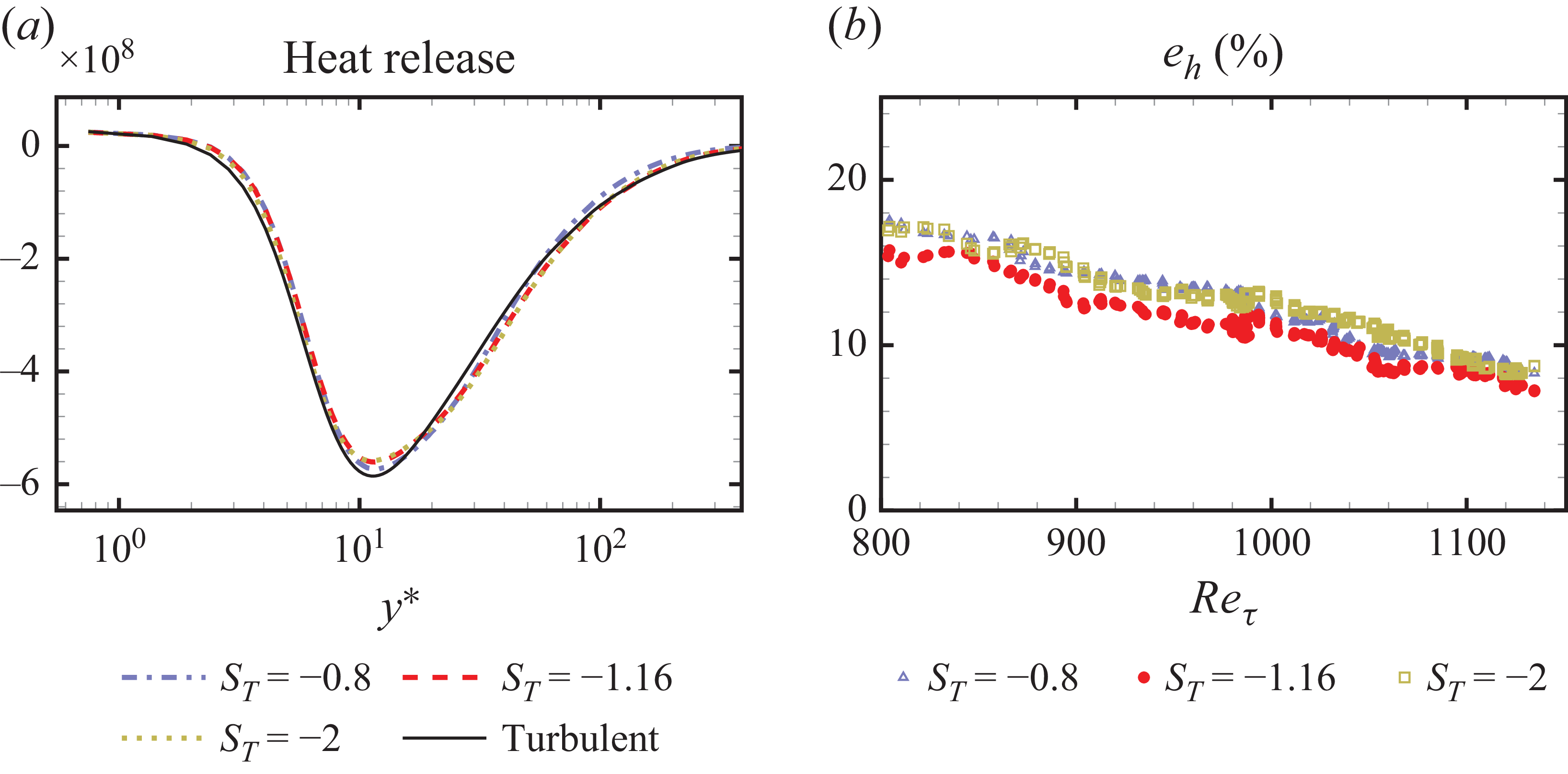
observed in previous data, including both boundary layers and channel flows under various flow conditions. Figure 17(a) shows that the wall-normal profiles of the heat release rate obtained for different
 $S_T$
align closely with each other. Furthermore, figure 17(b) demonstrates that using
 $S_T=-0.8$
or
 $S_T=-2$
, values differing from
 $S_T=-1.16$
evaluated from DNS, result in only a less than 4 % increase in the defined model error
 $e_h$
across different frictional Reynolds numbers.
Sensitivity study of log-normal closure to different model parameters
 $S_T$
. (a) Wall-normal profile of heat release rate. (b) Error metrics
 $e_h$
against the frictional Reynolds number
 $\textit{Re}_\tau$
. Here
 $S_T=-1.16$
is the parameter value used in previous results shown in figures 13( f) and 14(a).

In summary, the turbulent closure results show limited sensitivity to the exact value of
 $S_T$
, provided that a negative value within
 $-2\lt S_T\lt -0.8$
is prescribed. This range covers the values observed in our simulated and exploited databases. However, employing values closer to zero would result in significant errors, as the log-normal distribution then resembles a symmetric distribution, leading to unsatisfactory closure results, as shown in figure 14. Analysis of the channel flow databases with varying Mach numbers and wall temperatures indicates that
 $S_T$
remains negative in the near-wall region, with its precise value primarily dependent on the wall temperature.
A preliminary guideline for prescribing this model parameter beyond the present flow conditions is as follows: we recommend referring to figures 12(a), 15 and 16 in selecting an appropriate
 $S_T$
for the considered flow conditions, before transforming it to the equivalent constant
 $c_m$
using (4.11) and obtaining the required upper-bounded temperature
 $T_{\textit{max}}$
through (4.9). Nevertheless, this guideline is only preliminary and several challenges remain in providing a universal one for prescribing
 $S_T$
. The wall-normal distribution of temperature skewness is inherently non-uniform. Presently, only within the configuration in this paper has it been shown that assuming a uniform value equal to the peak yields satisfactory turbulent closure. It remains to be determined whether this assumption is valid in other flow settings. Ultimately, a non-uniform wall-normal distribution of temperature skewness might be required in some configurations. Moreover, while the dependence of temperature skewness on wall temperature was analysed using channel flow databases, its behaviour may differ in boundary layer flows, particularly in the outer region. These limitations require further investigation using existing or future DNS databases of reacting turbulent boundary layers.
Performance of log-normal closure with errors in temperature variance. Results are shown for deviations of −20 %, −10 %, 0 %, 10 % and 20 % in the value of
 $T'$
. The 0 % case uses the exact temperature variance obtained from DNS, which is the same as the results presented in figures 13( f) and 14(a). (a) Wall-normal profile of heat release rate. (b) Error metric
 $e_h$
against the frictional Reynolds number
 $\textit{Re}_\tau$
.

4.5. Influence of computation error in temperature variance on model performance
While it is reasonable to use exact values from DNS in the development of closure model, the single second-order statistics required, the temperature variance
 $T'^2$
, may be particularly challenging to obtain with accuracy in practice, although various modelling strategies for temperature variance have been proposed in RANS modelling of combustion flows (Poinsot & Veynante Reference Poinsot and Veynante2005). To address this issue, an additional study is conducted to assess the influence of errors in the temperature variance on model performance. Specifically, errors of −20 %, −10 %, 0 %, 10 % and 20 % are imposed on the value of
 $T'$
, and the closure results are re-evaluated using exact values of the first-order statistics and
 $S_T=-1.16$
from DNS data. Figure 18 indicates that model performance deteriorates in the presence of such errors; nevertheless, all results remain superior to the laminar closure, as quantified by the defined metric
 $e_h$
. An overestimated value of
 $T'$
results in excessive chemical heat absorption, as the resulting PDF extends over a higher temperature range that predominantly contributes to heat release. Conversely, an underestimated
 $T'$
produces heat absorption profiles that approach those of the laminar closure. It can be concluded from figure 18 that deviations of −10 % to 10 % in
 $T'$
still yield acceptable closure results under the present flow condition.
5. Analysis of the turbulent closure effect in a wall model
We analyse the effect of turbulent chemical closure in a wall model for wall-modelled large-eddy simulation (LES) of a compressible boundary layer with chemical non-equilibrium effects. In wall-modelled LES, the turbulent flow is resolved in the outer region of the boundary layer, while the near-wall region, where the characteristic length and time scales are too small for practical LES resolution, is represented through a wall model. Wall models introduce reduced forms of the near-wall equations, often expressed as ordinary differential equations (ODEs) derived under equilibrium or quasiequilibrium assumptions. Those ODEs are posed as initial value problems whose solutions must match the LES-resolved variables at the interface between the modelled inner layer and the resolved outer layer. The formulation and numerical solution of those reduced near-wall equations, together with the matching conditions, constitute the key elements of wall-model development.
The wall-model equations have strong links with the RANS equations, because the inner-layer system can be interpreted as a one-dimensional, steady, streamwise-averaged reduction of the compressible RANS boundary-layer equations closed with turbulent models. As a consequence, the structure of model equations, as well as the dependence on turbulence transport closures, corresponds directly to those appearing in conventional RANS formulations, despite posed as an ODE system in the wall-normal coordinate.
For reacting boundary-layer flows, a coupled ODE system of momentum, energy and species balance equations is required (Di Renzo & Urzay Reference Di Renzo and Urzay2019; Muto et al. Reference Muto, Daimon, Shimizu and Negishi2019; Cogo et al. Reference Cogo, Williams, Griffin, Picano and Moin2023). Using a mixture-averaged diffusion coefficient together with a gradient-diffusion model for turbulent species transport, the species balance equation is written as
 \begin{equation} \dfrac {\rm d}{{\rm d}y}\left [\left(\bar {\rho }\bar {D}_i + \dfrac {\bar {\mu }_t}{Sc_{t,i}}\right)\dfrac {{\rm d}\tilde {Y}_i}{{\rm d}y}\right ] + \bar {\dot {\omega }}_i= 0, \end{equation}
where
 $D_i$
is the mixture-averaged molecular diffusion coefficient for species
 $i$
(Hirschfelder, Curtiss & Bird Reference Hirschfelder, Curtiss and Bird1964),
 $Sc_{t,i}$
is the turbulent Schmidt number of species
 $i$
, and
 $\mu _t$
is the eddy viscosity. The reduced near-wall species equation describes the balance between molecular and turbulent diffusive fluxes and the local chemical source term. Under non-catalytic conditions with zero species flux at the wall, integration of the species equation yields
 \begin{equation} \frac{\textrm{d}\tilde{Y}_i}{\textrm{d}y} =\frac{\displaystyle \int_0^{y} -\bar{\dot{\omega}}_i \textrm{d}y} {\displaystyle \bar{\rho}\bar{D}_i + \frac{\bar{\mu}_t}{\textit{Sc}_{t,i}}}, \end{equation}
which shows that the turbulent mean chemical reaction rate
 $\bar {\dot {\omega }}_i$
directly controls the gradients of species mass fractions in the inner layer. The reaction rate enters as an integrated quantity from the wall to a given wall-normal location, which motivates the use of an integrated error metric for turbulent chemical closure in (4.12).
Wall-normal profiles of species mass fraction gradients based on (5.2). The left-hand side of (5.2) is computed from DNS (black dashed line). The right-hand side,
 $({\rm d}\tilde {Y_i}/{\rm d}y )_{RHS}= \int _0^{y} -\bar {\dot {\omega }}_i {\rm d}y / (\bar {D}_i + \bar {\mu }_t / Sc_{t,i})$
, is evaluated using the turbulent mean reaction rates from DNS, the log-normal closure and the laminar closure.

An a priori evaluation of (5.2) is performed using the non-catalytic DNS dataset to examine the predicted species gradients based on mean reaction rates obtained with different closure methods. The turbulent Schmidt numbers are identified to be approximately 0.9 for all species across the boundary layer, except in the region
 $y^*\lt 10$
where molecular diffusion dominates; therefore,
 $Sc_{t,i}=0.9$
is used for all five species. The eddy viscosity
 $\mu _t$
is determined from the DNS mean velocity field through the near-wall shear stress relation
 $(\bar {\mu }+\bar {\mu }_t) {\rm d}\tilde {U}/{\rm d}y = \tau _w$
(Cogo et al. Reference Cogo, Williams, Griffin, Picano and Moin2023). Figure 19 shows that the log-normal closure produces species gradient predictions that are closer to the DNS profiles for all five species compared with the laminar closure. Quantitative differences between the log-normal closure and DNS remain; however, similar deviations also appear when the DNS turbulent reaction rate is used directly, indicating that the reduced species balance equation contains modelling errors independent of the chemical closure approach. For atomic nitrogen, the laminar closure yields a positive gradient, in conflict with the DNS results. The log-normal closure improves the near-wall prediction by capturing the increase in atomic nitrogen, but does not reproduce the weakly negative gradient farther from the wall. For this species, the left- and right-hand sides of the species balance equation exhibit nearly exact agreement when the mean turbulent reaction rate extracted from DNS is used.
In practice, the species balance equation is solved together with the momentum and energy balance equations (Di Renzo & Urzay Reference Di Renzo and Urzay2019; Muto et al. Reference Muto, Daimon, Shimizu and Negishi2019). The inverse velocity transformation and the velocity–enthalpy relation are also applied to enhance the robustness of the wall model performance (Cogo et al. Reference Cogo, Williams, Griffin, Picano and Moin2023; Griffin, Fu & Moin Reference Griffin, Fu and Moin2023). In this study, the compressible velocity transformation and the velocity–enthalpy relation have been validated in figures 4 and 24, respectively. Since the focus of this work is on the effect of chemical closure, only the non-catalytic species balance (5.2) is solved by determining the wall-species mass fractions
 $\tilde {Y}_{w,i}$
that yield the best agreement with the prescribed wall-model/LES interface values. The temperature statistics and the eddy viscosity are treated as frozen, using the DNS profiles. In other words, (5.2) is integrated from
 $\tilde {Y}_{w,i}$
with the mean reaction rates
 $\bar {\dot {\omega }}_i$
and diffusion coefficients
 $\bar {D}_i$
varying along the wall-normal direction as functions of
 $\tilde {Y}_{i}$
. The solution is obtained via a shooting method, where a Newton iteration is employed, using a weighted-averaged of species errors as the residual and the numerically evaluated Jacobian matrix. The wall-normal interface location is denoted as
 $y_c^*$
.
Some trial attempts show that the convergence of atomic nitrogen is highly sensitive to the prescribed initial values
 $\tilde {Y}_{w,i}$
when closure models are used instead of the exact mean turbulent reaction rates from DNS. This issue is further examined by forward integration of (5.2) to
 $y_c^*=30$
using the DNS values of
 $\tilde {Y}_{w,i}$
. Figure 20 shows that the laminar closure produces an exponential growth of atomic nitrogen, resulting from the incorrect positive gradient predicted in figure 19(d). As a consequence, the reaction rates of the other species computed with the laminar closure differ substantially from the DNS reference at
 $y_c^*=30$
. The log-normal closure combined with the DNS value of
 $\tilde {Y}_{w,\mathrm{N}}$
leads to an early decrease of atomic nitrogen, yielding zero nitrogen away from the wall (red dashed line). To examine the sensitivity to
 $\tilde {Y}_{w,\mathrm{N}}$
, the atomic nitrogen profile is recomputed with
 $1.05 \tilde {Y}_{w,\mathrm{N}}$
, which yields an incorrect species growth for
 $y^*\gt 10$
(green dashed line). Both incorrect profiles obtained with the log-normal closure are consistent with the behaviour in figure 19(d), associated with the early drop to a negative gradient and a slightly positive gradient farther from the wall. While convergence for atomic nitrogen can still be obtained using a fine-grid search over the initial value
 $\tilde {Y}_{w,\mathrm{N}}$
, the strong sensitivity of
 $\tilde {Y}_{\mathrm{N}}$
at
 $y_c^*=30$
to this initial value makes the Jacobian-based shooting method difficult to converge. Computations using the turbulent reaction rate for atomic nitrogen, together with the log-normal closure for the other species (black dashed line), result in close agreement with the DNS nitrogen profile. Although neither the laminar nor the log-normal closure captures the nitrogen profile accurately, the log-normal closure yields clear improvement relative to the laminar closure, as seen from the mass fraction profiles of the other four species, which show correct tendency with respect to the DNS results.
Wall normal profiles of species mass fractions obtained by forward integration of (5.2) from the DNS wall values
 $\tilde {Y}_{w,i}$
to interface
 $y_c^*=30$
, with one additional log-normal computation using
 $1.05\tilde {Y}_{w,N}$
(green dashed line).

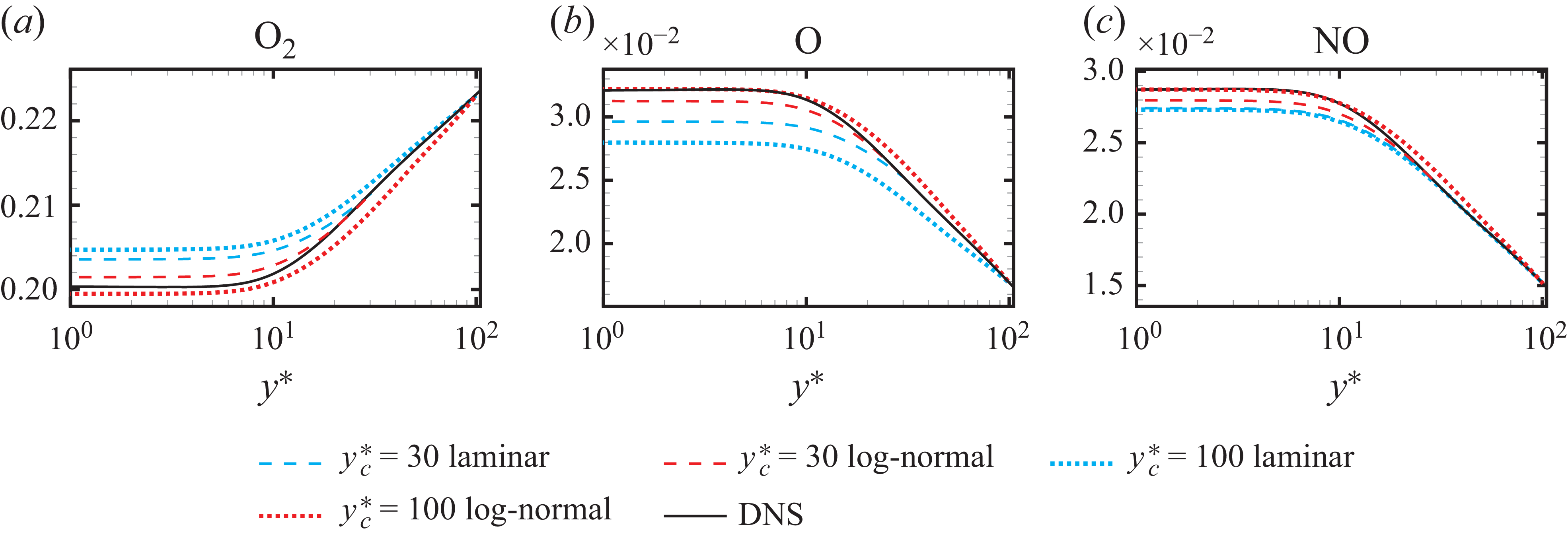
We compare the wall model performance using log-normal and laminar closures at two interface locations,
 $y_c^*=30$
and
 $y_c^*=100$
. A shooting method is applied to compute the species profiles for
 $\mathrm{O}_2$
,
 $\mathrm{O}$
,
 $\mathrm{NO}$
and
 ${N_2}$
, while the profile of
 $\mathrm{N}$
is taken from DNS due to the convergence issue discussed above. Figure 21 shows that the log-normal closure provides improved profile values at the wall surface and at around
 $y^*\approx 10$
where the reaction rates reach their maximum. Such an improvement is achieved at both interface locations. This behaviour is consistent with the numerical experiment of Cogo et al. (Reference Cogo, Williams, Griffin, Picano and Moin2023), in which shooting-method computations using the frozen DNS turbulent reaction rates yield closer agreement with the reference profiles than the laminar closure; in this paper, however, the reaction rates are further obtained through the log-normal closure and dynamically updated at each iteration. Future modelling developments for the closure of
 $\mathrm{N}$
will be required for a robust wall model computation, potentially involving empirical constraints or numerically bounded treatments.
Wall normal profiles of species mass fractions computed using the shooting method at two interface locations,
 $y_c^*=30$
and
 $y_c^*=100$
. The profile of
 $\mathrm{N}$
is taken from DNS and is not shown. The profile of
 ${N_2}$
is omitted due to the mass fraction summation constraint.

6. Discussion
6.1. On the choice of assumed PDF model as closure strategy
For the specific closure problem of finite-rate endothermic reaction in high-speed boundary layers, this work employs the PDF approach rather than the others developed for turbulent combustion (as discussed in § 1). We now justify our choice of the assumed PDF approach over the transported PDF method.
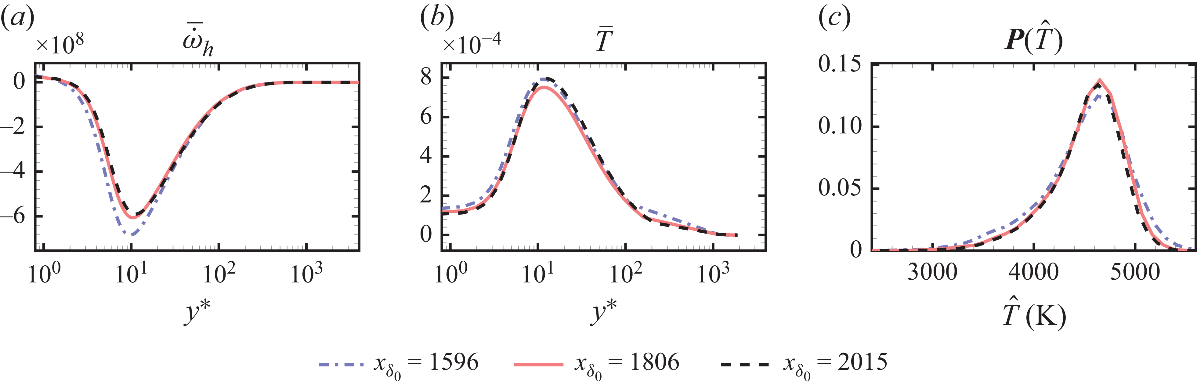
First, flow quantities in developed turbulent boundary layers are nearly homogeneous in the streamwise direction. While turbulent flame configurations often require transport PDF approaches to capture strongly varying local PDF shapes, the similarity in turbulent boundary layer offers the possibility to scale flow quantities across different streamwise positions. Figure 22(a,b) shows that wall-normal peak positions of mean heat release and temperature at different streamwise locations collapse when scaled with
 $y^*$
. Figure 22(c) further shows that the temperature PDF at wall-normal positions of maximum heat absorption exhibits resembling shape at various streamwise positions. By definition, the assumed PDF can be employed if a fixed shape of PDF can eventually be assumed, which is the case here due to the quasiparallel development of turbulent boundary layer.
Wall-normal profiles of mean heat release rate (a), mean temperature (b) and temperature PDF associated with maximum heat absorption at different streamwise positions.

Second, turbulence–chemistry interaction weakly affects temperature fluctuations, which remain dominated by turbulent mixing. The interaction Damköhler number of several orders below unity, reported in Duan & Martin (Reference Duan and Martin2011a
), Passiatore et al. (Reference Passiatore, Sciacovelli, Cinnella and Pascazio2021) and Di Renzo & Urzay (Reference Di Renzo and Urzay2021), confirms that fluid dynamics occur much faster than the rate difference in chemical reactions to be modelled. Thus, chemical source terms influence temperature and species fluctuations non-instantaneously compared with turbulent mixing. Indeed, those chemical source terms can have long-time effect, but they do not substantially alter temperature statistics profiles (figure 6) and temperature–velocity correlations (Appendix A). Comparisons between figures 12(a) and 16(b) reveal nearly identical peak skewness values, for non-reacting channel flows and reacting boundary layers at similar wall/recovery temperature ratios. This similarity can be extended even to non-reacting incompressible flows where temperature acts as a passive scalar (Antonia et al. Reference Antonia, Krishnamoorthy and Fulachier1988; Nagano & Tagawa Reference Nagano and Tagawa1988; Li et al. Reference Li, Schlatter, Brandt and Henningson2009), indicating that turbulent mixing primarily governs temperature statistics. As noted by Poinsot & Veynante (Reference Poinsot and Veynante2005) for slow
 $\mathrm{NO}_x$
formation in burnt gases where kinetics depend mainly on temperature, our similarly temperature-controlled reactions in high-speed boundary layers is considered suitable with assumed PDF modelling.
Third, one of the most important difficulties in assumed PDF method is the modelling of multivariable JPDF distributions. While techniques exist specific configurations like unconfined diffusion flames (Janicka & Kollmann Reference Janicka and Kollmann1979; Bockhorn Reference Bockhorn1988; Landenfeld et al. Reference Landenfeld, Sadiki and Janicka2002; Baurle & Girimaji Reference Baurle and Girimaji2003), constructing spatially varying high-dimensional PDFs proves impractical for most turbulent flames, and the transport PDF approach is preferred. In contrast, our results shows that it is possible to reduce the multivariable PDF to a single-variable PDF on temperature, which considerably avoids the difficulty of constructing high-dimensional PDF and the associated transport equations for species fluctuations.
Finally, since the application of present closure model is targeted for RANS of hypersonic vehicles at full scale, computational efficiency is an important consideration, particularly for three-dimensional RANS simulations. The transport PDF approach, while providing more accurate and complete statistical information, requires greater computational resources, due to the need to solve the joint velocity-composition PDF commonly achieved using Monte Carlo methods. The assumed PDF approach is less cost-demanding and has demonstrated significant improvements in the present configuration.
6.2. Model applicability
The present closure model is developed based on DNS data corresponding to a maximum mean temperature around 5000 K, using the five-species Park’s model, consistent with state-of-art DNS calculations of spatially developing turbulent boundary layers (see table 3). The chosen five-species model is considered suitable for flow temperatures below 6000 K, where the effect of ionisation can be neglected (Di Renzo & Urzay Reference Di Renzo and Urzay2021). While more complex reaction models, such as 11-species models (Dunn & Kang Reference Dunn and Kang1973; Park Reference Park1989), exist, we do not recommend applying our proposed closure models to those more complex chemical reactions in RANS calculations. The closure of mean reaction rates associated with new elementary reaction steps, which has not been verified through DNS data, may introduce significant errors in the mean chemical source terms.
The use of non-catalytic and supercatalytic conditions has represented a range of wall-species conditions. However, we note that gas–surface interactions (Gupta Reference Gupta1996) linked to ablation effects (Başkaya et al. Reference Başkaya, Dungan, Hickel and Brehm2024a , Reference Başkaya, Capriati, Turchi, Magin and Hickelb ; Zhao et al. Reference Zhao, Zuo, Wang, Yuan and Wen2024) could significantly alter the first- and second-order statistics of species concentrations in the near-wall region, which may cover the wall-normal positions of maximum heat absorption. In such scenarios, the JPDF may not be able to reduce to a single-variable PDF, necessitating a multivariable PDF approach.
Performing RANS with the proposed turbulent closure should consider only translational temperature, since vibrational non-equilibrium has not been accounted for in the employed DNS data. In the formulation of a two-temperature model, with translational and vibrational temperature denoted as
 $T_S$
and
 $T_V$
, respectively, a geometrically averaged temperature
 $T_{\textit{a}v\textit{g}}=T_S^q T^{1-q}_V$
is applied for reactions R1–R3, where
 $q=0.7$
(Park Reference Park1988; Passiatore et al. Reference Passiatore, Sciacovelli, Cinnella and Pascazio2022). In such cases, turbulent closure should be analysed for each elementary reaction step to determine whether modelling
 $T_{\textit{a}v\textit{g}}$
and
 $T_S$
independently for different reaction steps remain valid.
7. Conclusions
High-speed and low-altitude flight regimes result in turbulent external flow at high temperatures, leading to reacting turbulent flows with dissociative chemical non-equilibrium effects. The RANS-based methods are employed to simulate hypersonic vehicles at full scales; however, the turbulent chemistry closure in RANS is omitted due to the lack of closure models, which can be a source of error introduced to the simulated results. This paper proposes a simple closure model for turbulent chemistry of air dissociation reactions in high-speed boundary layers, leveraging PDF methods for turbulent combustion modelling.
The study is based on DNS of a hypersonic turbulent boundary at Mach 9.2 with an isothermal cold wall surface using Park’s five-species finite-rate reaction model. Three sets of DNS are conducted, including two chemically reacting setting with non-catalytic and supercatalytic wall surface conditions, and one non-reacting run. The DNS results are validated against reference calculations at similar flow parameters. The effects of wall-catalysis and chemical reactions on turbulent statistics are examined. The magnitudes of reaction rates under supercatalytic conditions are found to be less than those under non-catalytic reactions across the boundary layer, due to the cancellation of chemical reaction rates at the cold wall surface. Chemical reaction slightly reduces the Reynolds normal stresses, but weakly increases the skin friction by a maximum ratio below 6.5 %, attributed to a modulation effect of wall shear strain. A more significant impact of chemical reactions was observed on temperature statistics, where both the magnitudes of temperature averages and fluctuations were reduced. These trends, consistent with those observed in adiabatic conditions (Passiatore et al. Reference Passiatore, Sciacovelli, Cinnella and Pascazio2021), demonstrate slight but non-negligible errors potentially introduced by the lack of turbulent chemistry modelling.
Through the definition and evaluation of diagnostic reaction rates, we identify that the temperature fluctuations have a primary impact on the turbulence–chemistry interaction of the air dissociation reaction under consideration. This finding indicates that knowledge of only the mean values of species concentrations, with an accurate modelling of the temperature PDF, is sufficient to achieve a satisfactory closure of turbulent reaction rates. This removes the complexity of modelling a multivariable PDF and paves the way for applying an assumed PDF modelling approach. However, the temperature PDF in the near-wall region exhibits a skewed distribution similar to passive scalar PDFs in incompressible channel flows, which is not as straightforward as a Gaussian or Beta distribution. We find that employing a log-normal distribution for the temperature PDF, with inputs of temperature mean values and variance, can effectively close the turbulent chemical source terms. This approach reduces the error magnitude, defined across the boundary layer, by more than 45 % compared with laminar closure, for both non-catalytic and supercatalytic surfaces.
The single model parameter to be calibrated from DNS is the temperature skewness
 $S_T$
, which is selected to approximate its value in the inner layer to achieve a good approximation of maximum heat absorption. The dependence and sensitivity of temperature skewness are further investigated using compressible channel flow databases (Yu et al. Reference Yu, Xu and Pirozzoli2019; Yu & Xu Reference Yu and Xu2021). It is found the temperature skewness remains negative within the near wall region across a wide range of Mach numbers and wall temperatures. The exact value of temperature skewness is little dependant on Mach numbers, but varies with wall temperature, which is interpreted as a turbulent transport effect. The accuracy of the closure results is not strongly sensitive to the exact chosen value of
 $S_T$
; within the range
 $-2\lt S_T\lt -0.8$
covering the peak skewness values observed in all exploited data, changes in defined model error are less than 4 %. The sensitivity of model performance to inaccuracies in the temperature variance,
 $T'^2$
, is also evaluated. The results show that an error of −10 % to + 10 % in
 $T'$
relative to its DNS value still yields acceptable predictions.
The proposed turbulent closure model is applied to a multispecies reacting wall model (Di Renzo & Urzay Reference Di Renzo and Urzay2019; Cogo et al. Reference Cogo, Williams, Griffin, Picano and Moin2023), with emphasis on the analysis of species balance equations where the averaged chemical reaction rate appears. The log-normal closure provides clear improvements over the laminar closure in both the a priori evaluation of species gradients and the shooting-method computations of wall species mass fractions. For the atomic nitrogen profile, although the log-normal closure performs substantially better than the laminar closure, it still produces species gradients that differ from the DNS results. This discrepancy leads to strong sensitivity of the nitrogen profile to its initial value and makes the Jacobian-based shooting method difficult to converge unless a fine-grid search for the initial value is employed. Note that two-dimensional and three-dimensional RANS computations share a similar near-wall species balance with the ODEs in the examined one-dimensional wall model, and therefore the impact of this closure inaccuracy in RANS requires further investigation.
We note that the current model is restricted to a maximum mean temperature of approximately 5000 K without ionisation, consistent with recent DNS studies (Di Renzo & Urzay Reference Di Renzo and Urzay2021; Passiatore et al. Reference Passiatore, Sciacovelli, Cinnella and Pascazio2022). Future model development is planned to incorporate more complex physical phenomena, such as vibrational non-equilibrium and gas–surface reactions linked to ablation. Nonetheless, we expect the proposed closure strategy and the developed model to be applicable in related RANS studies, enhancing the calculation of near-wall statistics affected by the finite-rate chemical non-equilibrium effects of air dissociation.
Acknowledgements
We express our gratitude to an anonymous reviewer of Wang & Xu (Reference Wang and Xu2024), for suggesting PDF methods in the analysis of turbulence–chemistry interactions. We thank X.-L. Li for providing the OpenCFD-Comb code, and F.-Z. Lv for sharing the postprocessing code for vortex identification. We thank Griffin et al. (Reference Griffin, Fu and Moin2023) for sharing their MATLAB code in the supplementary material, which provided a valuable reference for developing the species-balance wall model in § 5. We appreciate the reviewers’ suggestions to improve the paper.
Funding
The work is supported by the National Natural Science of China (grant nos. 12302286, 12388101). C.–H.W. is supported by the Shuimu postdoc fellowship from Tsinghua University.
Declaration of interests
The authors report no conflict of interest.
Mean temperature and velocity scaling, superposed by Walz scaling in (A1). Here Walz-
 $T$
uses
 $f(\tilde {u}/u_e)=\tilde {u}/u_e$
, whereas Walz-
 $T$
-modified uses the correction
 $f( \tilde {u}/u_e )=f_m( \tilde {u}/u_e )$
. Here
 $\textit{Re}_\tau =1135$
for the non-catalytic, catalytic and non-reacting cases.

Appendix A. Correlations of temperature and velocity statistics under chemical reactions
The relation between mean velocity and temperature is investigated and compared with the scaling proposed by Walz (Reference Walz1969), which reads
 \begin{equation} \dfrac {\tilde {T}}{T_e}=\dfrac {T_w}{T_e}+\dfrac {T_r-T_w}{T_e}f\! \left ( \dfrac {\tilde {u}}{u_e} \right )+\dfrac {T_e-T_r}{T_e} \left (\frac {\tilde {u}}{u_e} \right )^2\!. \end{equation}
For the expression of
 $f( \tilde {u}/u_e )$
, Walz originally derived that
 $f(\tilde {u}/u_e)=\tilde {u}/u_e$
. Duan & Martin (Reference Duan and Martin2011b
) subsequently proposed a correction for non-adiabatic wall surfaces by fitting to DNS data, yielding
 $f( \tilde {u}/u_e )=f_m( \tilde {u}/u_e )=0.1741(\tilde {u}/u_e)^2+0.8259(\tilde {u}/u_e)$
. Figure 23 indicates that chemical reactions and wall catalysis do not have a strong influence on the mean velocity–temperature scaling. However, both the original Walz formula and the modified version with
 $f=f_m$
fail to reproduce the DNS scaling, a discrepancy attributed to the assumption of a calorically perfect gas (Duan & Martin Reference Duan and Martin2011b
; Passiatore et al. Reference Passiatore, Sciacovelli, Cinnella and Pascazio2022). To address this, Duan & Martin (Reference Duan and Martin2011b
) proposed an enthalpy-based scaling without the perfect-gas assumption, expressed as
 \begin{equation} \dfrac {\tilde {h}}{h_e}=\dfrac {h_w}{h_e}+\dfrac {h_r-h_w}{h_e} f\! \left ( \dfrac {\tilde {u}}{u_e} \right )-r\dfrac {0.5 u_e^2}{h_e}\left ( \dfrac {\tilde {u}}{u_e} \right )^2\!, \end{equation}
where the recovery enthalpy is analogously written as
 $h_r=h_e+0.5 r u_e^2$
. The enthalpy-based scaling with
 $f=f_m$
exhibits improved agreement with DNS data for both non-catalytic and catalytic cases, as shown in figure 24. Note that the wall enthalpy
 $h_w$
differs between these cases because the species compositions are not identical.
Mean enthalpy and velocity scaling, superposed by enthalpy-based Walz scaling in (A2) with the correction
 $f( \tilde {u}/u_e )=f_m( \tilde {u}/u_e )$
: (a) non-catalytic; (b) catalytic.

Wall normal profiles of turbulent Prandtl numbers. Non-catalytic, catalytic and non-reacting cases at
 $\textit{Re}_\tau =1135$
.

The turbulent Prandtl number
 $\textit{Pr}_t$
is commonly employed to model turbulent heat transport in RANS equations, and is defined as
 \begin{equation} \textit{Pr}_t=\dfrac {\overline {\rho u'' v''} \partial \tilde {T} }{\overline {\rho v'' T''} \partial \tilde {u} }. \end{equation}
Evaluation of DNS data demonstrates that chemical reactions have little influence on the wall-normal profiles of
 $\textit{Pr}_t$
, as shown in figure 25. The profiles exhibit values of approximately
 $\textit{Pr}_t=0.5$
in the linear regime, and vary from
 $\textit{Pr}_t=1$
to
 $\textit{Pr}_t=0.6$
in the outer layer. The apparent discontinuity in the profile is attributed to the near-vanishing turbulent heat flux
 $\overline {\rho v'' T''}$
at the location of peak mean temperature, a feature that has also been reported in cold-wall configurations (Duan, Beekman & Martin Reference Duan, Beekman and Martin2010; Di Renzo & Urzay Reference Di Renzo and Urzay2021).


The validity of the strong Reynolds analogy (SRA), which relates temperature and velocity fluctuations, is assessed using DNS data. The original form of SRA (Morkovin Reference Morkovin1962) is expressed as
 \begin{equation} \dfrac {T_{\textit{rms}}''/\tilde {T}}{(\gamma -1)Ma^2 (u_{\textit{rms}}''/\tilde {u})}=1. \end{equation}
Figure 26(a) indicates that the original formulation yields values below 0.5 in the outer layer, a behaviour typical of cold-flow conditions (Duan et al. Reference Duan, Beekman and Martin2010; Duan & Martin Reference Duan and Martin2011b ). Several extensions of the SRA have also been examined, including the GHSRA proposed by Duan & Martin (Reference Duan and Martin2011b ), given by
 \begin{equation} T_{\textit{rms}}''=-\dfrac {1}{\textit{Pr}_t}\dfrac {\partial \tilde {T}}{\partial \tilde {u}} u_{\textit{rms}}''. \end{equation}
This formulation generalises the HSRA expression (Huang, Coleman & Bradshaw Reference Huang, Coleman and Bradshaw1995) by removing the calorically perfect gas assumption. As shown in figure 26(b), it provides good agreement with unity in the outer layer. The other examined extensions do not show better agreement and they are not shown for simplicity. Nevertheless, both the original SRA and the GHSRA are found to be invalid close to the wall, consistent with cold-flow observations (Duan et al. Reference Duan, Beekman and Martin2010; Duan & Martin Reference Duan and Martin2011b ). In practice, this limitation should be carefully considered when modelling temperature fluctuations.
Diagnostic heat release rates defined in (4.3) and (4.4):
 $\breve {\dot {\omega }}_h|_{\bar {Y}_{{\rm O_2}}}$
,
 $\breve {\dot {\omega }}_h|_{\bar {Y}_{\mathrm{O}}}$
,
 $\breve {\dot {\omega }}_h|_{\bar {Y}_{\mathrm{NO}}}$
,
 $\breve {\dot {\omega }}_h|_{\bar {Y}_{\mathrm{N}}}$
,
 $\breve {\dot {\omega }}_h|_{\bar {Y}_{\mathrm{N}_2}}$
(a–e) and
 $\breve {\dot {\omega }}_h|_{\bar {T}}$
( f). The same profiles of turbulent and laminar heat release rates,
 $\overline {\dot {\omega }}_h (T,\boldsymbol{Y})$
and
 $\dot {\omega }_h (\overline {T},\overline {\boldsymbol{Y}})$
, are provided in each panel. Catalytic data results are presented, corresponding to non-catalytic data in figure 9.

Chemical source terms modelled with
 $\boldsymbol{P}(\hat {T})$
from DNS, as defined in (4.5) and (4.6):
 $\tilde {\dot {\omega }}_{{\rm O_2}}$
,
 $\tilde {\dot {\omega }}_{\mathrm{O}}$
,
 $\tilde {\dot {\omega }}_{\mathrm{NO}}$
,
 $\tilde {\dot {\omega }}_{\mathrm{N}}$
,
 $\tilde {\dot {\omega }}_{{\rm N_2}}$
(a–e) and
 $\tilde {\dot {\omega }}_h$
( f) . The associated turbulent source terms
 $\overline {\dot {\omega }}_i (T,\boldsymbol{Y})$
,
 $\overline {\dot {\omega }}_h (T,\boldsymbol{Y})$
and the laminar source terms
 $\dot {\omega }_i (\overline {T},\overline {\boldsymbol{Y}})$
,
 $\dot {\omega }_h (\overline {T},\overline {\boldsymbol{Y}})$
are superposed. Catalytic data results are presented, corresponding to non-catalytic data in figure 10.

Chemical source terms modelled with
 $\boldsymbol{P}(\hat {T})$
of the log-normal distribution, as defined in (4.5), (4.6) and (4.7):
 $\tilde {\dot {\omega }}_{{\rm O_2}}$
,
 $\tilde {\dot {\omega }}_{\mathrm{O}}$
,
 $\tilde {\dot {\omega }}_{\mathrm{NO}}$
,
 $\tilde {\dot {\omega }}_{\mathrm{N}}$
,
 $\tilde {\dot {\omega }}_{{\rm N_2}}$
(a–e) and
 $\tilde {\dot {\omega }}_h$
( f). The associated turbulent source terms and the laminar source terms are superposed in each panel. Catalytic data results are presented, corresponding to non-catalytic data in figure 13.

Appendix B. Turbulent chemical closure results with the supercatalytic condition
Turbulence–chemistry interaction analysis using supercatalytic data is provided in the appendix. Figures 27, 28, 29 present the results under supercatalytic conditions, corresponding to those under non-catalytic conditions in figures 9, 10, 13, respectively. The wall-normal profiles are extracted at the same streamwise position,
 $x_{\delta _0}=2015$
, as the non-catalytic case. No qualitatively different results are observed between both catalytic conditions and a good closure can also be achieved. Note that the error metrics evaluated under supercatalytic conditions were presented in figure 14(b).