


Introduction
Ice-penetrating-radar images, ice-core records and ice deformation measurements hold clues to past and future behavior of ice sheets. The challenge is to infer paleoclimate and ice-flow history from these data. Rigorous solution of these inverse problems requires an understanding of the subtleties of ice deformation and flow.
Ice cores are often drilled near ice divides, in order to minimize stratigraphic disturbance due to horizontal shearing of ice (e.g. Reference Waddington, Bolzan and AlleyWaddington and others, 2001). Therefore, a rigorous ice-flow model for the ice-divide region is required, particularly since, at ice divides, longitudinal stress gradients cannot be ignored (Reference NyeNye, 1959; Reference Morland and JohnsonMorland and Johnson, 1980; Reference RaymondRaymond, 1983). Furthermore, at the low deviatoric-stress levels found under ice divides, the ice rheology may be near-linear, changing the pattern of ice flow (Reference Waddington, Raymond, Morse and HarrisonWaddington and others, 1996; Reference Pettit and WaddingtonPettit and Waddington, in press). Ice flow can also be influenced by changing boundary conditions. For example, there is a significant feedback between the near-divide flow field and the surface temperature (Reference HvidbergHvidberg, 1996). Elevation changes of bounding ice streams (Reference Nereson, Hindmarsh and RaymondNereson and others, 1998b), or transient and spatially asymmetric accumulation-rate patterns (Reference Nereson, Hindmarsh and RaymondNereson and others, 1998a) can cause an ice divide to migrate.
Here, we explore the effects of basal motion on the ice-flow pattern and the internal stratigraphy under an ice divide. Some ice divides are presently frozen to their beds (e.g. Greenland Summit (Reference Johnsen, Dahl-Jensen, Dansgaard and GundestrupJohnsen and others, 1995); Devon Island, Canada (Reference Paterson and ClarkePaterson and Clarke, 1978); and Siple Dome, West Antarctica (personal communication from G. Clow, 2001) ), while others such as Law Dome, Antarctica (Reference Budd, Young and AustinBudd and others, 1976), and parts of the West Antarctic Ross–Amundsen ice divide (Morse and others, in press) are at or near the pressure-melting temperature at the bed. At these divides, basal sliding, a deforming-till layer, or both, may be present.
Because polar ice is described by a power-lawconstitutive relation, (e.g. Reference PatersonPaterson, 1994, ch. 5, “Glen’s Law”), its “effective viscosity” increases with decreasing effective deviatoric stress. Where an ice sheet is frozen to its bed, the deep ice directly under a divide experiences low deviatoric stress, has a relatively high effective viscosity, and is relatively resistant to deformation. As a result, stratigraphic layers tend to move downward more slowly within a distance of one ice thickness of the ice divide, when compared to flank regions (at distances greater than about five ice thicknesses from the divide). In a steady state, these layers tend to form an arch (“Raymondbump”) in the divide region (Reference RaymondRaymond, 1983). However, when the basal ice can slide, or when a deformable-till layer exists, stresses are redistributed, and the deep ice undergoes more longitudinal extension. This extension increases longitudinal deviatoric stress in the deep ice under the divide, resulting in a lower effective viscosity there and a weakened tendency to form a Raymond bump.
In order to explore the effects of various levels of basal sliding on the flow pattern and the stratigraphy, we must first formulate a realistic spatial pattern of basal motion that might be expected under and near ice divides. This is not a trivial matter, because there is still no general agreement on the detailed form of a basal sliding relationship for ice sheets. Conventional sliding boundary conditions incorporate simplifications and assumptions that break down in the divide region. Many models incorporate a sliding law based on the theory by Reference WeertmanWeertman (1957), for which sliding velocity, ub, is a function of local basal-shear stress (Reference NyeNye, 1959; Reference Morland and JohnsonMorland and Johnson, 1980; Reference PaynePayne, 1995; Reference Marshall, Tarasov, Clarke and PeltierMarshall and others, 2000; Reference Tarasov and PeltierTarasov and Peltier, 2000):

where τ is the local shear stress, and k is a function of several ice-flow and geometric parameters, potentially including effective water pressure (the difference between ice overburden pressure and basal water pressure). As Reference WeertmanWeertman (1961) noted, this law includes the implicit assumption that longitudinal stresses are insignificant. Near an ice divide, however, longitudinal stresses cannot be neglected, because shear stresses approach zero. Because the driving shear stresses are small, we expect that longitudinal strain rates in the ice will control the allowable gradients in basal sliding velocity.
Here we use a two-dimensional plane-strain finite-element flow model, which automatically incorporates longitudinal-coupling effects. To parameterize sliding at the ice–bedrock interface, we use a layer of deformable, linearly viscous till and allow the model to determine the pattern of basal motion under and near a divide. We then vary the till viscosity to examine the sensitivity of isochrone shape and the velocity field to varying amounts of basal“sliding”. From the perspective of the ice, varying the till-layer thickness has the same effect as varying the till viscosity. Using a linearly viscous till, rather than a power-law till, will affect subtle details of the model results, but not the general features that we present here.
Finite-Element Ice-Flow Model
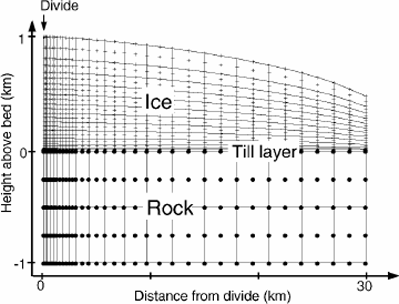
To calculate the velocity field and find the steady-state isochrone pattern, we use a thermomechanically coupled finite-element model (FEM). This model is similar to ice-divide models by Reference RaymondRaymond (1983) and Reference HvidbergHvidberg (1996). Figure 1 shows the model geometry.
FEM geometry. Solid lines are element (nine-node quadrilaterals) boundaries. Plus signs mark nodes in the ice. Solid dots mark bedrock nodes.The ice is initially 1000 m thick at the divide, with an initial surface profile calculated using the shallow-ice approximation.The ice at the divide can move only vertically. The velocity profile on the flank boundary (∽30Hdiv) exports ice flux equal to the surface accumulation integrated over the surface. The till layer is 10 m thick (one element thick).The ice-till and the till-rock contact are no-slip boundaries. In each model run, the surface evolves until it reaches steady state with the uniform accumulation rate.
The model is structured around the following assumptions:
-
1. The ice deforms in plane strain; thus, the model best represents a ridge ice divide, such as Siple Dome (Reference Nereson and WaddingtonNereson and others, 1996) or Roosevelt Island, West Antarctica (Reference Conway, Hall, Denton, Gades and WaddingtonConway and others, 1999).
-
2. Strain rate is a power-law function of deviatoric stress according to Glen’s flow law:
-
where ἑij and τij are the strain-rate and deviatoric-stress tensors, respectively, τeff is the effective deviatoric stress (Reference PatersonPaterson, 1994, p. 91) and we assume that A depends only on temperature through the Arrhenius relation A = A0 exp–Q/RT).
-
3. The ice is underlain by a layer of till of uniform thickness. There is no slip between the ice and the top of the till layer, and no slip between the bottom of the till and the bedrock. The viscosity of the till layer is a model input parameter which can be adjusted to model various levels of basal resistance.
-
4. The temperature calculation is based on the surface temperature and the geothermal gradient at the bottom of a thick layer of bedrock (Reference WaddingtonWaddington, 1987). In addition to conduction and advection, strain heating is included in the thermal model. The thermal conductivities and diffusivities of the ice, rock and till are assumed to be equal and uniform (the values for ice fall within the range typical for sedimentary rocks (Reference Stein and AhrensStein, 1995)).
-
5. The upper surface is stress-free and is allowed to evolve until a steady state is reached with a specified uniform accumulation rate. We define steady state as a maximum change in the surface elevation (excluding the five nodes nearest the flank boundary) over 1year of less than a specified tolerance є (typically <5 mma–1 for a 1000 m thick ice sheet).
-
6. The divide is a line of symmetry where ice is constrained to move only vertically.
-
7. The horizontal-velocity profile on the flank boundary (at 30 ice thicknesses from the divide) carries away the integrated mass balance from the divide to the boundary, in order to satisfy mass conservation for a steady-state ice sheet. Because our boundary is >20 ice thicknesses from the divide, the results for the region within 10 ice thicknesses of the divide are insensitive to the details of the horizontal-velocity profile on the flank boundary (Reference RaymondRaymond, 1983; Reference Schøtt, Waddington and RaymondSchøtt and others, 1992).
-
8. Because our goal was to isolate the effect of sliding, the layer of till does not undergo the thinning that one would expect, given the export of till by shearing flow through the flank boundaries. We also do not allow for mass loss due to melting from the base of the ice sheet or mass gain due to freeze-on of basal water.

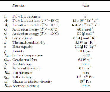
Table 1 shows values of constants used in the model. We chose the surface temperature, geothermal flux, ice thickness and accumulation rate characteristic of Siple Dome.
Model parameters
As shown in Figure 1, we model an idealized symmetrical divide with a flat bed. We use a 39 x 31-node grid of quadratic elements. Since we are most interested in the solution near the divide, the nodes are more closely spaced within the divide region. Horizontal ice velocity and horizontal temperature gradient are zero at the ice divide. The model solves for temperature, pressure and velocity fields.
We varied the till viscosity from 106 to 1015 Pas, to capture the range of possible behaviors. For each till viscosity, the model reaches a steady state in which the accumulation rate and the flow due to gravity (a function of the model geometry) are balanced. In order to compare different model runs, we chose to keep the accumulation rate constant and to allow for differences in the final steady-state geometry. The alternative is to maintain constant ice-sheet thickness at the divide, but adjust the accumulation rate for each set of boundary conditions. Our conclusions do not depend on this choice.
We present our results in non-dimensional form, indicated by a hat (–) over the variable. We use ice thickness at the divide, Hd iv , as the characteristic distance. The characteristic viscosity, ηice, is defined by rearranging Equation (2) for n = 3 such that τ = 2ηἑ (the standard form for a linear fluid). This yields (Reference Pettit and WaddingtonPettit and Waddington, in press):

Results
We use the value of A appropriate for average ice temperature. ἑchar = ḃ/Hdiv, where b is the accumulation rate. The characteristic time is tchar = 1/ἑchar = Hd iv/ḃ. For Siple Dome, the characteristic viscosity is ηice = 1010 Pas (η̂ice = 1) and the characteristic time is tchar = 104 years.
Our first goal was to determine a realistic spatial distribution of basal-ice motion under an ice divide. To do this we used a layer of till with an adjustable but spatially uniform viscosity and thickness. When ice is frozen to its bed, the entire ice flux has to be transported through internal deformation in the ice. A very stiff till layer produces the same results. But as the viscosity of the till layer decreases, shear deformation in the till increases, decreasing the shear deformation required within the ice sheet to achieve equilibrium with the specified accumulation rate at the surface. Ultimately, when the till viscosity is low enough, virtually all of the shear deformation is concentrated in the till layer, shear stress at the base of the ice goes to zero, and the ice deforms only through longitudinal stretching (similar to an ice shelf). This trend is shown in Figures 2 and 3.
Longitudinal profile ofvelocity at the till–ice contact, and (b) the surface profile, for a range of non-dimensional till viscosities. The non-dimensional viscosity of Siple Dome ice at –15° C is 1(explained in the text).
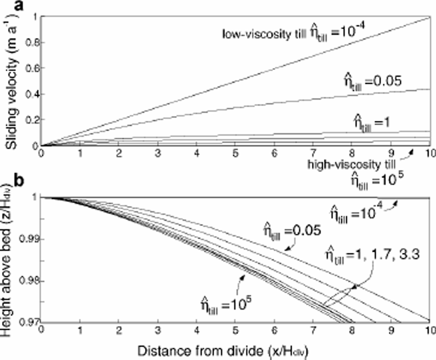
“Sliding velocity” is represented by the basal ice motion at the ice–till contact. Figure 2a shows the longitudinal profile of this basal ice motion for model runs with a range of non-dimensional till viscosities η–till from 10–4 to 105. In the low-viscosity-till model run, the basal-ice motion increases linearly with distance from the divide. This result is not unexpected, since nearly all of the motion occurs through shearing of the till layer. In this case, longitudinal stress σ̂xx in the overlying ice, which varies slowly with distance from the divide, controls the basal-velocity gradient. The ice near the divide moves away from the divide as “plug flow” (Fig. 3a): the basal velocity in this region is equal to the surface velocity, which, from steady-state mass continuity, is

Vertical- and horizontal-velocity profiles at 0, 0.25H, 0.5H, 1H, 2H, 4H and 10H from the divide (as indicated by the curve labels) for three model runs: (a) low-viscosity till, (b) medium-viscosity till and (c) high-viscosity till.

where x is the distance from the divide. In contrast, in the high-viscosity-till model run (Fig. 3c), sliding velocity is zero everywhere, and the ice motion is accommodated largely through internal horizontal simple shear. In both of these cases, the details of the rheology of our till layer do not affect the results.
To conserve mass, the plug-flow horizontal-velocity profile of the weak-till model run requires a near-linear vertical velocity profile at all distances from the divide, as shown on the left side of Figure 3. The ice sheet necessarily reaches a different steady-state surface profile in plug flow compared to a steady state dominated by internal deformation in the ice (Fig. 2b). In steady state, the ice flux at any position is equal to the integrated accumulation rate from the ice divide; this flux is the same regardless of the till viscosity. Therefore, as till viscosity decreases, increased basal sliding contributes more to the ice flux, and the internal deformation within the ice sheet must contribute less. Since internal deformation is driven by ice thickness and slope, a steady ice sheet with more sliding must be thinner and have a shallower slope.
We also explored the behavior of the flow and stratigraphy with basal-till viscosities intermediate between the stiff-till (η̂till = 105) and weak-till (η̂till = 10–4) model runs. The velocity field and steady-state geometry of an ice sheet are most sensitive to the till viscosity when the till viscosity is within an order of magnitude of the characteristic ice viscosity (η̂ ice = 1). For these transitional model runs, the total deformation is divided comparably between the till and the ice. The sliding velocities and surface profiles for these intermediate model runs are shown in Figure 2. Unlike the result in the weak-till model run, these velocity profiles are not linear (Fig. 2a). The sliding velocity gradually increases with distance from the divide, with a steeper gradient within a few ice thicknesses of the divide. The horizontal-velocity profile is more similar to plug flow near the divide; however, as surface slope and basal shear stress increase with increasing distance from the divide, internal deformation carries an increasing fraction of the ice flux (Fig. 3b). The details of the model results for these transitional model runs depend on our choice of till rheology. A power-law till would slightly change the curvature of the sliding velocity and surface-profile curves in Figure 2.
To maintain the plug flow characteristic of the low-viscosity-till model run (and the near-divide zone of the transitional model runs), the longitudinal deviatoric stresses must be more evenly distributed with depth, compared with the pattern for an ice sheet frozen to its bed. This is particularly important near the base of the ice at the divide, where low deviatoric stresses and correspondingly high effective ice viscosity (due to the non-linearity of Glen’s flow law) contribute to the formation of the Raymond bump in the isochrones. In Figure 4, we show results from four model runs with non-dimensional till viscosities varying from 105 to 10–4. The left column shows simulated steady-state isochrones, and the right column shows the pattern of non-dimensional effective viscosity in the ice. Figure 4a shows the typical patterns for an ice sheet frozen to its bed. The arch in the isochrones on the left results from deformation around the “hard” zone deep under the divide, as seen in the effective-viscosity distribution on the right. All three of the high- to moderate-viscosity till model runs (a–c) show a zone of relatively hard ice deep under the divide. The extent of this zone and the magnitude of its peak effective viscosity relative to the viscosity on the flank determines the size of the Raymond bump; as we increase basal sliding, the arch in the isochrones diminishes.The high longitudinal stresses near the bed of an ice sheet with basal sliding keep the effective viscosity low (Fig. 4d), and hinder the formation of this zone, resulting in flatter isochrones.
Isochrones and effective viscosities for four model runs with decreasing till viscosity (dark shading represents low effective viscosities; light shading represents high viscosities). The size of the Raymond bump is related to the ice viscosity peak at the base of the ice at the divide relative to the flank (more than about five ice thicknesses away from the divide). (a) High till viscosity (f,m =105); (b) moderate till viscosity (η̂till=1.7); (c) till viscosity (f,m =1); (d) low till viscosity (f,m =10–4). (a–c) have similar flank viscosities; (d) has a slightly higher flank viscosity because the steady-state ice sheet is somewhat thinner and therefore is colder. Note that (b) and (c) have similar till viscosities, yet measurably different viscosity peaks and Raymond bump sizes; this is evidence that the transition from hard-till end member (a) to soft-till end member (d) occurs over a small range of till viscosities. The isochrones near the bed for the transitional model runs show a slight down-warping. This is a subtle effect of our choice of linear till rheology and is not likely to occur in a real ice sheet.

By analyzing the decrease in prominence of the divide arch, we can quantify the effect of sliding on the flow field. We define the amplitude ofthe Raymondbump for each isochrone as the maximum distance that the isochrone rises above an imaginary smooth curve that best fits the shape of the isochrone onboth flanks of the dome. In Figure 5, this arch amplitude is plotted as a function of the fractional height of the isochrone at 10 ice thicknesses from the divide for each model run. The arch decreases in magnitude with increasing sliding. Also, the depth of its maximum amplitude decreases as sliding increases. This effect is due to a subtle change in the shape of the vertical velocity profile at the divide (see Fig. 3). The depth of a layer is given by the temporal integral of its downward velocity along its particle path. The maximum arch amplitude occurs at a depth where the difference between these integrals is maximum for particle paths at the divide and on the flank. As the amount of basal sliding increases, the differences between flank and divide vertical-velocity profiles are pushed to shallower depths; this subtle shape change pushes the height of the maximum amplitude upwards.
In Figure 6 we take each curve from Figure 5, and plot the maximum bump amplitude against the flank flux ratio qs, defined as the percentage of the total ice flux carried by sliding at about five ice thicknesses from the divide:

Variation in arch amplitude (relative to the ice-sheet thickness) with height above bed for several model runs. The dashed part of the curves indicates a rough extrapolation to the surface and the bed (the curves should approach the surface and bed with infinite slope).

Relationship between the maximum Raymond-bump amplitude for each model run (“×”; plotted relative to the stiff-till model run) and the ratio of sliding to total flux at a distance of five ice thicknesses from the divide. The curve is an exponential fitted to the data points.
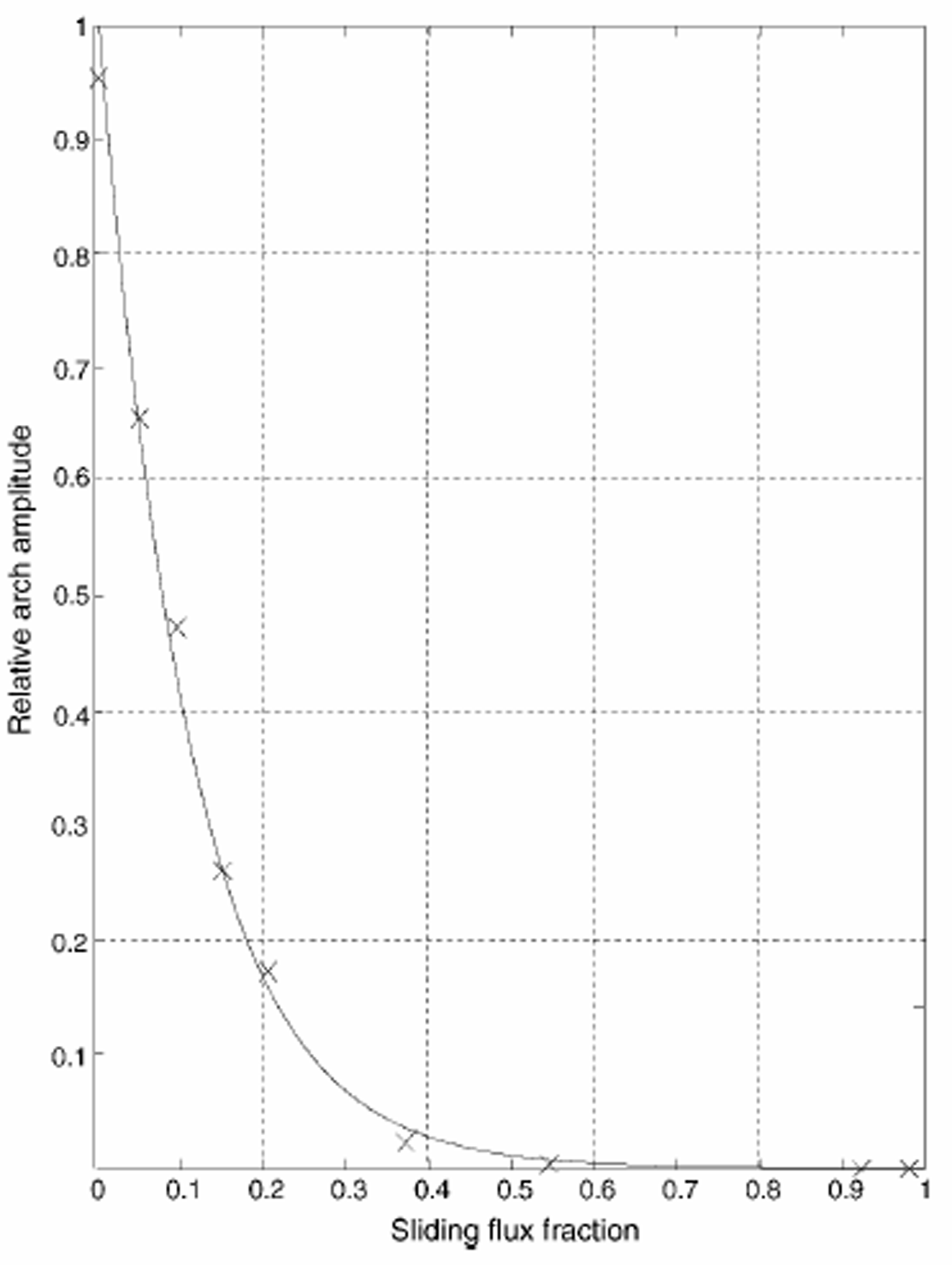
where H5 is the ice thickness at 5Hdiv, ub is the sliding velocity at 5Hdiv, and ui is the horizontal velocity due to internal deformation at 5Hdiv. Figure 6 shows that the maximum arch amplitude decays exponentially with increasing sliding: it takes only 11% sliding flux to cause the arch to decrease to 36% (1/e) of its size in the stiff-till model run. Thus, a small amount of sliding can significantly alter ice flow and reduce the amplitude of the Raymond bump.
Discussion
Previous attention to sliding has focused on fast-moving ice streams and on the central reaches of valley glaciers. The impact of sliding on the flow pattern near ice divides has received little attention. To our knowledge, only Reference Morland and JohnsonMorland and Johnson (1980) have looked in some detail at the effect of sliding on the flow field near an ice divide. They assumed a sliding velocity based on a modification of Equation (1), which we expect has difficulty in reflecting the important role of longitudinal-stress gradients near a divide. Because the overlying ice resists dramatic inhomogeneities in longitudinal strain rate, the basal-ice velocity should also vary smoothly with position. Reference WeertmanWeertman (1961), realizing that Equation (1) may be inapplicable near a divide, added a longitudinal-stress term, and showed that, as a result, small ice caps such as the Barnes were predicted to have a flatter profile than the sliding law (Equation (1)) would suggest.
To investigate the effect of sliding at a divide more thoroughly, we have incorporated a layer of deformable till into our plane-strain finite-element ice-flow model. Our till layer is not intended to be a realistic basal substrate, but it is a simple method for representing sliding behavior that includes the strong longitudinal-stress coupling represented by extensional stresses in the ice. Indeed, for low-viscosity till, the sliding velocity near the divide is controlled by the longitudinal strain rate in the ice, not by the details of processes in the till. Furthermore, with a“slippery” ice–rock interface instead of a till layer, the results should be the same. Also, the longitudinal coupling in the ice will smooth out stress variations due to roughness or small topographic features.
Although we present results for a steady-state ice sheet, ice divides that are undergoing changes are probably never far from the steady-state stress and flow patterns that we derive (e.g. Reference Nereson, Waddington, Raymond and JacobsonNereson and Waddington, 2002). This allows us to use our results to address changes in flow and stratigraphy as an ice sheet evolves. For example, Reference Conway, Hall, Denton, Gades and WaddingtonConway and others (1999) used the stratigraphy observed by ice-penetrating radar in the vicinity of the divide on Roosevelt Island to infer that, prior to 3200 years ago, Roosevelt Island did not exhibit the special flow pattern that is characteristic of an ice divide frozen to its bed (Raymond, 1983). They also went on to infer that Roosevelt Island was not an ice divide prior to 3200 BP; it may have been on the slope of a larger ice sheet. While the latter inference may be correct, our results suggest that an alternate interpretation is possible. Prior to 3200 BP, Roosevelt Island could have supported an ice divide over a wet bed that allowed sliding; if, at 3200 BP, the basal ice on Roosevelt Island then froze to the bedrock, the special ice-divide flow pattern that is creating the observed transient Raymond bump would have been initiated. The ice on Roosevelt Island appears to have thinned by several hundred meters since 3200 BP (Reference Conway, Hall, Denton, Gades and WaddingtonConway and others, 1999). Comparable thinning prior to 3200 BP would have tended to cool the basal ice and, if it was thawed, could have led to freezing.
Conclusion
In this modeling study, we find that basal-ice motion under a divide in plane strain is likely to exhibit a roughly linear increase with distance from the divide if the ice–bed interface is slippery. The basal motion is limited not by shearing in the till but by longitudinal stretching within the ice.
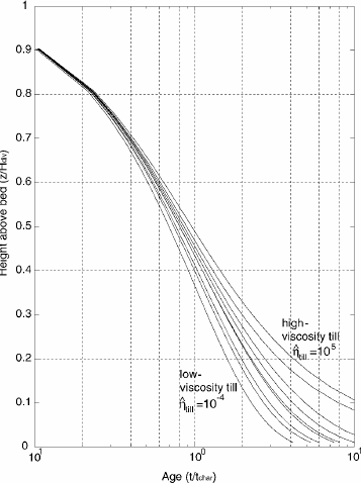
The shapes of the horizontal- and vertical-velocity profiles are more uniform with distance from the divide when the basal ice is allowed to slide; the unique divide flow described by Reference RaymondRaymond (1983) disappears. This creates flatter isochrones and a younger depth–age scale. As the sliding contribution increases, the vertical-velocity pattern (Fig. 3) and the depth–age distribution (Fig. 7) approach their corresponding patterns on the flank. In addition, as the flux fraction due to basal motion is increased, the longitudinal and vertical strain rates become more uniformly distributed over depth. As a result, the ice experiences greater downward flow at all intermediate depths, creating younger depth–age relationships as shown in Figure 7.
Depth–age scale at the ice divide for varying till viscosities. Since the final steady-state geometries are slightly different, we use non-dimensional time t = t̂/tchar. The depth–age scales for all model runs at a location on the flank fall on the same curve as the low-viscosity till model run.
The history of basal sliding is an important factor in the interpretation of ice-penetrating radar layers and depth– age scales for ice-core records at ice divides.
Acknowledgements
We thank C. F. Raymond and H. Conway for discussions. We also thank A. Fowler (Scientific Editor) and F. Ng (referee) for their suggestions and discussions, and T. Hulbe (referee) for her comments. This work was supported by NSF OPP9615417, NSF OPP9726113 and a U.S. National Science Foundation Graduate Research Fellowship to E. C. Pettit.



