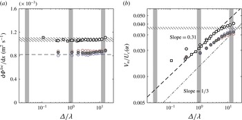
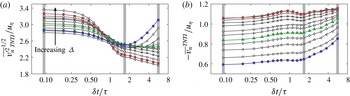
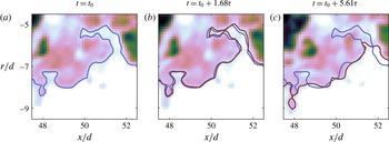
1 Introduction
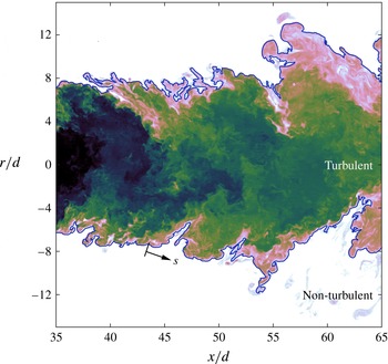
A thorough understanding of turbulent entrainment has been a long-standing challenge in fluid mechanics. Turbulent entrainment represents the transport of non-turbulent fluid across the boundary between the turbulent and non-turbulent regions of a flow. The turbulent entrainment process and the mechanisms that control the transport of mass, momentum, and scalars from a turbulent region of a fluid to a non-turbulent region are also of widespread interest in science and engineering. The early studies of Brown & Roshko (Reference Brown and Roshko1974), Dahm & Dimotakis (Reference Dahm and Dimotakis1987) and Liepmann & Gharib (Reference Liepmann and Gharib1992) attributed entrainment to the role of large-scale eddies in a process known as engulfment, in which parcels of irrotational fluid are enveloped by large-scale turbulent structures and brought into contact with turbulent fluid. However, later investigations by Mathew & Basu (Reference Mathew and Basu2002), Westerweel et al. (Reference Westerweel, Fukushima, Pedersen and Hunt2005), Taveira et al. (Reference Taveira, Diogo, Lopes and da Silva2013), and others did not find significant amounts of unmixed fluid within the turbulent fluid (see figure 1). Similarly, da Silva, Taveira & Borrell (Reference da Silva, Taveira and Borrell2014) report that ‘bubbles’ of irrotational fluid that are found inside of the turbulent region are the same as the weakly rotational pockets of fluid found within fully developed isotropic turbulence simulations. These findings indicate that entrainment predominantly happens at the edges of the turbulent/non-turbulent interface (TNTI) rather than inside the turbulent core. More generally, there is some ambiguity when ascribing a length scale to engulfment processes (e.g. encasing parcels of unmixed fluid), because this process is difficult to measure and quantify. For clarification, in this paper we define engulfment as a predominantly inviscid entrainment process that is characterised by its association with large-scale motions.
Instantaneous scalar concentration field of the far field of a turbulent jet at
 $Re=25\,300$
, shown in logarithmic contour scaling. The TNTI is denoted by the blue line, and the coordinate along the TNTI,
 $s$
, is also presented. Note the absence of unmixed fluid within the jet.

There is much greater consensus that viscous and molecular diffusion at the smallest scales near the TNTI is responsible for the transfer of vorticity and scalar concentration to irrotational and unmixed fluid, respectively: a process known as viscous nibbling. The concept of viscous nibbling was first suggested by Corrsin & Kistler (Reference Corrsin and Kistler1955), and has been supported by simulations and experiments by Mathew & Basu (Reference Mathew and Basu2002), Westerweel et al. (Reference Westerweel, Fukushima, Pedersen and Hunt2005), da Silva & Taveira (Reference da Silva and Taveira2010), Holzner & Lüthi (Reference Holzner and Lüthi2011), Taveira et al. (Reference Taveira, Diogo, Lopes and da Silva2013), and Wolf et al. (Reference Wolf, Holzner, Lüthi, Krug, Kinzelbach and Tsinober2013). These studies have shown that irrotational fluid particles in the non-turbulent region of the flow acquire vorticity near the TNTI over length, velocity and time scales that are representative of the smallest scales of the flow. However, it is also important to note that the local entrainment rate along the TNTI is in fact decorrelated from the local dissipation field (Holzner & Lüthi Reference Holzner and Lüthi2011). In other words, local entrainment along the TNTI proceeds at the smallest scales of the flow, but it is not strongly influenced by the small-scale turbulence.
If the local entrainment is decoupled from the small-scale turbulence, then it is perhaps reasonable to expect that a full description of the entrainment process will need to account for multi-scale interactions, as suggested by Sreenivasan, Ramshankar & Meneveau (Reference Sreenivasan, Ramshankar and Meneveau1989), Mathew & Basu (Reference Mathew and Basu2002), Philip & Marusic (Reference Philip and Marusic2012), and van Reeuwijk & Holzner (Reference van Reeuwijk and Holzner2014). Townsend (Reference Townsend1976, p. 232) provides a succinct description of entrainment as a multi-scale process:
[T]he development of vorticity in previously irrotational fluid depends in the first place on viscous diffusion of vorticity across the bounding surface. Since the rate of entrainment is not dependent on the magnitude of the fluid viscosity, the slow process of diffusion into the ambient fluid must be accelerated by interaction with the velocity fields of eddies of all sizes, from the viscous eddies to the energy-containing eddies so that the overall rate of entrainment is set by large-scale parameters of the flow.
In this regard, we cannot rule out the influence of the large scales on entrainment; we may only rule out the physical process of ‘engulfing’ parcels of fluid. However, as stated earlier, it is not straightforward to delineate the role of the large scales on entrainment. For example, along the TNTI in a turbulent jet and a shear-free flow, it has been shown that the inviscid contribution to entrainment is much weaker than the viscous contribution (Holzner & Lüthi Reference Holzner and Lüthi2011; Wolf et al. Reference Wolf, Lüthi, Holzner, Krug, Kinzelbach and Tsinober2012). In comparison, other researchers have found evidence that suggests that the large scales influence the overall entrainment rate in a range of turbulent flows. Moser, Rogers & Ewing (Reference Moser, Rogers and Ewing1998) report a larger growth rate in a forced-temporal wake compared to the unforced case. Forcing induces large-scale modulations in the topology of the shear layers, and therefore increases the surface area of the TNTI (e.g. Bisset, Hunt & Rogers Reference Bisset, Hunt and Rogers2002, Mathew & Basu Reference Mathew and Basu2002). Similarly, Krug et al. (Reference Krug, Holzner, Lüthi, Wolf, Kinzelbach and Tsinober2015) observed a greater entrainment rate in an unstratified flow compared with a stratified flow; they also attributed this greater entrainment rate to the increased surface area of the TNTI. Conversely, altering the smallest scales of the flow by changing the viscosity does not modify the overall entrainment rate (Townsend Reference Townsend1976). The influence of the large scales on entrainment was also observed by Philip & Marusic (Reference Philip and Marusic2012), who applied a large-scale hairpin model, in a manner similar to Nickels & Marusic (Reference Nickels and Marusic2001), that was able to recover the mean entrainment rate in a round, turbulent jet. The hairpin model correctly predicted the radial inflow of non-turbulent fluid, which determines the overall entrainment rate, despite neglecting the small scales of the flow. These studies allude to an entrainment process in which viscous nibbling adjusts to the imposed entrainment rate defined by the large scales of turbulence. One way in which the large scales may modulate the entrainment rate is to generate a large surface area over which viscous nibbling may act to mix the turbulent and non-turbulent fluid (Mathew & Basu Reference Mathew and Basu2002).
1.1 The multi-scale nature of the TNTI surface area
The multi-scale nature of turbulence may be characterised from a fractal perspective. Mandelbrot (Reference Mandelbrot1982) describes fractal self-similarity as ‘[invariance] under certain transformations of scale’. One result of this self-similarity is the non-trivial scaling of the area of a turbulent surface as a function of the measurement resolution. This surface scaling (or contour scaling in two dimensions) is commonly measured using box-counting techniques; this technique is described in § 4.1. It is suggested that there is an intermediate range of scales between the dissipation scales and the inertial scales over which the box count along a turbulence isosurface scales as
 $N\sim \unicode[STIX]{x1D6E5}^{-D_{3}}$
, where
 $\unicode[STIX]{x1D6E5}$
is the box side length and
 $D_{3}$
is a universal fractal dimension (e.g. Sreenivasan & Meneveau Reference Sreenivasan and Meneveau1986). The first experimental evidence to support the fractal nature of turbulence was presented by Sreenivasan & Meneveau (Reference Sreenivasan and Meneveau1986) and Sreenivasan et al. (Reference Sreenivasan, Ramshankar and Meneveau1989) for a range of shear flows such as jets, wakes, and boundary layers. However, these early experiments were performed at only moderate Reynolds numbers that were limited by a narrow scale separation, which introduces some ambiguity when attempting to establish a universal fractal dimension for any turbulent flow (Dimotakis & Catrakis Reference Dimotakis, Catrakis, Chaté, Villermaux and Chomaz1999; Catrakis Reference Catrakis2000). Another uncertainty is the apparent dependence of the threshold value of the interface, and the methods used to evaluate the fractal dimension (Sreenivasan Reference Sreenivasan1991; Zubair & Catrakis Reference Zubair and Catrakis2009). For these reasons, it has been suggested that the fractal dimension of a turbulent surface may be scale-dependent rather than exhibit a constant scaling (Miller & Dimotakis Reference Miller and Dimotakis1991; Catrakis & Dimotakis Reference Catrakis and Dimotakis1996). However, evidence of a scale-dependent fractal dimension may be attributed to finite
 $Re$
and effects from the large scales, amongst others (see Zubair & Catrakis Reference Zubair and Catrakis2009 and references therein). Addressing these concerns, work by de Silva et al. (Reference de Silva, Philip, Chauhan, Meneveau and Marusic2013) implemented high-resolution PIV, with a large dynamic range, to examine the scaling of the TNTI of a high-Reynolds-number turbulent boundary layer. de Silva et al. (Reference de Silva, Philip, Chauhan, Meneveau and Marusic2013) report that the fractal dimension of the TNTI is scale-independent and falls in the range
 $D_{3}=2.3$
to
 $2.4$
using a box-counting and a spatial-filtering technique. Similar fractal dimensions are also observed by Chauhan et al. (Reference Chauhan, Philip, de Silva, Hutchins and Marusic2014b
) in the TNTI of a turbulent boundary layer, and by Zubair & Catrakis (Reference Zubair and Catrakis2009) in separated shear layers but for general scalar isosurfaces. It has therefore not yet been resolved as to whether a constant fractal scaling exists in free-shear flows. One of the aims of this paper is to address this question for the case of an axisymmetric, turbulent jet.
1.2 Motivation for the present study
Whereas previous studies have primarily focused on the topology of the TNTI surface, in the present study we also consider the physical fluxes and rates of entrainment across the TNTI. This is achieved by considering the global and local entrainment in an axisymmetric, turbulent jet. The global entrainment is typically calculated using the mean TNTI surface area and the ensemble-averaged radial velocity (Morton, Taylor & Turner Reference Morton, Taylor and Turner1956). Comparatively, the local entrainment is typically calculated using the highly corrugated instantaneous TNTI surface area and the local entrainment velocity at each point along the surface; this definition of the net mass entrainment may be written as
 $\unicode[STIX]{x1D70C}V_{n}S$
. Here,
 $\unicode[STIX]{x1D70C}$
is the constant fluid density, which we shall henceforth ignore, and
 $S$
is the TNTI surface area. The mean entrainment velocity,
 $V_{n}=\overline{\iint (-v_{n})\,\text{d}a|_{TNTI}/\!\iint \text{d}a|_{TNTI}}$
, is the integral of the local entrainment velocity (
 $v_{n}$
) over the TNTI surface, which is then ensemble-averaged over many realisations (denoted by an overline,
 $\overline{(~)}$
). The local entrainment velocity is defined more precisely in § 2.5, but we simply note here that a negative
 $v_{n}$
implies mass flux into the turbulent region, or a positive entrainment. Measurement of
 $V_{n}$
has only recently become possible with direct numerical simulations (DNS) and high-resolution experiments (Holzner & Lüthi Reference Holzner and Lüthi2011; Wolf et al.
Reference Wolf, Lüthi, Holzner, Krug, Kinzelbach and Tsinober2012; van Reeuwijk & Holzner Reference van Reeuwijk and Holzner2014; Krug et al.
Reference Krug, Holzner, Lüthi, Wolf, Kinzelbach and Tsinober2015). For velocity fields on a two-dimensional (2D) axisymmetric plane in an axisymmetric jet, such as that studied in this paper, the mean entrainment velocity is approximated with
 $$\begin{eqnarray}V_{n}\equiv \overline{\left[\frac{\displaystyle \int _{0}^{L_{s}}(-v_{n})r_{I}\,\text{d}s}{\displaystyle \int _{0}^{L_{s}}r_{I}\,\text{d}s}\right]}.\end{eqnarray}$$
In this expression the integration is performed along the TNTI (schematically shown in figure 1), where
 $L_{s}$
is the length of the interface, and
 $r_{I}$
is the radial location of the TNTI; details regarding this 2D approximation are discussed later in the paper.
A multi-scale analysis is necessary to connect global and local entrainment. Indeed, the notion that entrainment is a multi-scale phenomena has been proposed by Meneveau & Sreenivasan (Reference Meneveau and Sreenivasan1990), who suggest that total flux across the TNTI should be constant and scale-independent,
 $$\begin{eqnarray}V_{n}^{\unicode[STIX]{x1D708}}S^{\unicode[STIX]{x1D708}}=V_{n}^{A}S^{A}=V_{n}(\unicode[STIX]{x1D6E5})S(\unicode[STIX]{x1D6E5})=\text{constant}.\end{eqnarray}$$
Here, the superscript
 $\unicode[STIX]{x1D708}$
represents the viscous flux, superscript
 $A$
represents the advective flux (at the ensemble-averaged mean-flow level), and
 $\unicode[STIX]{x1D6E5}$
is the filter size (see for example appendix D in Philip et al. (Reference Philip, Meneveau, da Silva and Marusic2014) for further details). In other words,
 $V_{n}^{\unicode[STIX]{x1D708}}$
is the mean entrainment velocity at the smallest scales (with the corresponding highly corrugated surface area,
 $S^{\unicode[STIX]{x1D708}}$
),
 $V_{n}^{A}$
is the mean entrainment velocity at the largest mean scales (with
 $S^{A}$
, the smooth mean surface area), and
 $V_{n}(\unicode[STIX]{x1D6E5})$
and
 $S(\unicode[STIX]{x1D6E5})$
the corresponding quantities at intermediate length scales. The scaling rate in (1.2) was tested by Philip et al. (Reference Philip, Meneveau, da Silva and Marusic2014), but they were not able to confirm it because of the effect of limited spatial resolution on their ‘indirect’ estimation of the entrainment velocity. In this paper we overcome this limitation by implementing an interface-tracking technique that directly measures the entrainment velocity and is unaffected by spatial resolution; this technique is detailed in § 2.5.
The primary aims of this paper are (i) to confirm the scale-independent mass-flux hypothesis (1.2); this not only requires high
 $Re$
, but also a high-resolution measurement system that is capable of interface tracking. Equation (1.2) illustrates the intrinsic roles of
 $S(\unicode[STIX]{x1D6E5})$
and
 $V_{n}(\unicode[STIX]{x1D6E5})$
in testing the scale-independent mass-flux hypothesis. For this reason, we also seek to (ii) understand the scaling of the TNTI surface area,
 $S$
, and to (iii) understand the scaling of the mean entrainment velocity,
 $V_{n}$
. Although the scaling of
 $S(\unicode[STIX]{x1D6E5})$
has been presented as a constant power-law (fractal) scaling, there is yet to be clear consensus on this finding, because of suggestions of a scale-dependent (non-constant) power-law scaling (e.g. Miller & Dimotakis Reference Miller and Dimotakis1991). We aim to use our high-
 $Re$
flow and novel measurement system to shed light on this matter. Examining the scaling of the mean entrainment velocity,
 $V_{n}$
, inherently leads us to look deeper into relationship between the local entrainment velocity (
 $v_{n}$
) and the radial position of the TNTI (
 $r_{I}$
), at multi-scales.
1.3 Organisation of the paper
To achieve these aims we have implemented a multi-scale technique that spatially filters the velocity and scalar fields, and evaluates the mass-flux rate at different length scales. The multi-scale approach requires a large-scale separation and a high dynamic range to capture it. This is achieved with the experimental set-up that is first described in § 2. We then discuss the identification criterion for the TNTI and the planar measurement of the local entrainment velocity,
 $v_{n}$
, along the TNTI. In § 3 a comparison is made between local and global descriptions of the mean entrainment rate in turbulent jets. Furthermore, we present an alternative method of calculating the entrainment rate in jets by considering a conditional velocity distribution at the TNTI; this is similar to the technique introduced by Chauhan, Philip & Marusic (Reference Chauhan, Philip and Marusic2014a
) for entrainment in turbulent boundary layers. The scaling of the TNTI length, mass flux, and entrainment velocity are presented in § 4. In this last section we confirm the hypotheses of Meneveau & Sreenivasan (Reference Meneveau and Sreenivasan1990) and Philip et al. (Reference Philip, Meneveau, da Silva and Marusic2014) that the entrainment velocity does indeed scale inversely to the TNTI length to give a scale-independent mass flux.
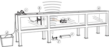
Schematic of the arrangement of (a) the water tank, (b) jet nozzle, (c) pumps, (d) dyed-fluid reservoir, (e) laser, (f) laser-sheet-forming optics, (g) PIV high-speed cameras, and (h) PLIF high-speed camera (not shown).

2 Experimental methods
2.1 Apparatus
Experiments were performed in a water tank
 $7~\text{m}$
in length with a cross section of
 $1~\text{m}\times 1~\text{m}$
and transparent acrylic side walls to provide optical access. A schematic is provided in figure 2. A round nozzle with an exit diameter
 $d=10~\text{mm}$
and flow conditioning via a series of wire meshes, honeycomb grid, and a fifth-order polynomial contraction was used to produce a top-hat velocity profile at the jet exit; the nozzle was positioned
 $520d$
away from the end wall of the tank. A separate reservoir containing dyed fluid for the scalar measurements was used in combination with a pump to supply the jet, which produced Reynolds numbers of
 $\mathit{Re}=25\,300$
(based on
 $d$
and
 $U_{e}$
, the average nozzle-exit velocity) and
 $\mathit{Re}_{\unicode[STIX]{x1D706}}=260$
(measured at the jet centreline, see table 1). A constant volumetric flow rate was maintained throughout the experiments, as determined from the pressure drop across a calibrated orifice plate. The streamwise, radial and spanwise coordinates are denoted by
 $x$
,
 $r$
and
 $z$
, with component velocities denoted by
 $u$
,
 $v$
and
 $w$
as usual. The scalar concentration is represented by
 $\unicode[STIX]{x1D719}$
.
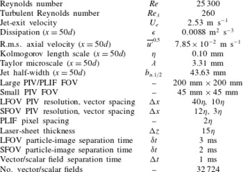
Experimental parameters and measured length, velocity and time scales of the turbulent jet. Note that here
 $Re=U_{e}d/\unicode[STIX]{x1D708}$
,
 $Re_{\unicode[STIX]{x1D706}}=\overline{u^{\prime }}^{0.5}\unicode[STIX]{x1D706}/\unicode[STIX]{x1D708}$
,
 $\unicode[STIX]{x1D716}=15\unicode[STIX]{x1D708}\overline{(\unicode[STIX]{x2202}u/\unicode[STIX]{x2202}x)^{2}}$
,
 $\unicode[STIX]{x1D702}=(\unicode[STIX]{x1D708}^{3}/\unicode[STIX]{x1D716})^{1/4}$
, and
 $\unicode[STIX]{x1D706}=u\sqrt{15\unicode[STIX]{x1D708}/\unicode[STIX]{x1D716}}$
; these quantities are measured at the jet centreline.

Two experimental set-ups of particle image velocimetry (PIV) and planar laser-induced fluorescence (PLIF) measurements were implemented. The first used a very large-scale field of view (FOV) to measure bulk flow characteristics that are presented in § 2.2. The second set-up used a multi-scale arrangement that was obtained using large-scale and small-scale FOVs, and is described in detail in § 2.3. This latter set-up is used to investigate the entrainment process in the turbulent jet.
2.2 Flow characterisation
Flow-characterisation experiments using PIV and PLIF are used to confirm that this flow does indeed follow classic scaling laws for free, turbulent jets. Even though these experiments are different from the experiments described in § 2.3, the set-up and processing methods are similar, and will be described in detail in § 2.3.
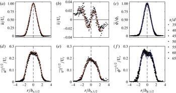
Figure 3 presents the normalised mean and r.m.s. velocity and scalar profiles in the far field of the jet. These profiles are measured across
 $30d$
of streamwise extent, starting from
 $x/d=35$
. There is very good collapse of the profiles when normalised by the jet half-width,
 $b_{1/2}$
, and they are also in good agreement with the mean profiles of Panchapakesan & Lumley (Reference Panchapakesan and Lumley1993), as denoted by the red lines in figure 3, and with the scalar profiles of Lubbers, Brethouwer & Boersma (Reference Lubbers, Brethouwer and Boersma2001), as denoted by the blue lines. The collapse of the mean and r.m.s. profiles across a span of streamwise distances indicates that the jet achieved self-similarity in the far field. The slight increase in the data scatter in the radial velocity profile,
 $\overline{v}/U_{c}$
, in figure 3(b) is an artefact of the coarse PIV measurement resolution rather than actual flow non-uniformities. Similarly, the slight asymmetry of the
 $\overline{{\unicode[STIX]{x1D719}^{\prime }}^{2}}^{1/2}$
profile (figure 3
f) is attributed to the attenuation of laser energy intensity through the fluorescent dye; the laser beam travels from the
 $r<0$
side of the jet. Corrections using the Beer–Lambert law are applied to the PLIF images, which yield the symmetric profile of
 $\overline{\unicode[STIX]{x1D719}}$
in figure 3(c). However, limitations of this normalisation technique becomes apparent when considering higher-order statistics. A similar asymmetry of the
 $\overline{{\unicode[STIX]{x1D719}^{\prime }}^{2}}^{1/2}$
profile has also been observed in comparable PLIF measurements of a turbulent jet by Fukushima, Aanen & Westerweel (Reference Fukushima, Aanen and Westerweel2002). The limitations of the PLIF image correction do not significantly affect the TNTI and entrainment velocity measurements in §§ 2.4–2.5 because the TNTI identification does not involve high-order scalar statistics, and the FOV only considers half of the radial extent that is shown in figure 3(c,f).
Self-similar profiles of the jet, normalised by the local centreline velocity (
 $U_{c}$
) and scalar concentration (
 $\unicode[STIX]{x1D719}_{c}$
), and the local jet half-width (
 $b_{1/2}$
); the radial location from the jet centreline is given by
 $r$
. Mean profiles of (a) axial velocity, (b) radial velocity, and (c) scalar concentration. Respective r.m.s. profiles of (d) axial velocity, (e) radial velocity, and (f) scalar concentration. The red lines denote the self-similar profiles reported in Panchapakesan & Lumley (Reference Panchapakesan and Lumley1993), and the blue lines denote the scalar profiles reported in Lubbers et al. (Reference Lubbers, Brethouwer and Boersma2001).

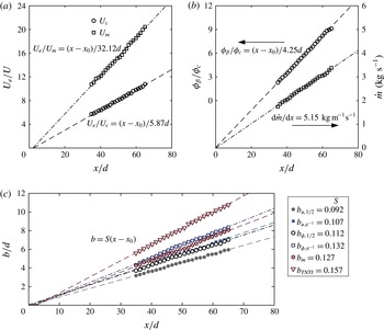
Further confirmation of the self-similar behaviour of the turbulent jet is presented in figure 4. As expected for free jets, the inverse of the centreline velocity,
 $U_{c}$
, in figure 4(a) scales linearly with streamwise distance,
 $x$
. The scaling coefficient for the centreline velocity (see Pope Reference Pope2000, p. 100) is
 $B=5.87$
, and is in good agreement with Hussein, Capp & George (Reference Hussein, Capp and George1994), who report
 $B=5.8{-}5.9$
. For comparison we also consider an integral measure of the velocity that is defined by
 $U_{m}=M/Q$
, where
 $M$
is the momentum flux and
 $Q$
is the volumetric flow rate. Variables
 $M$
and
 $Q$
are defined in appendix B. The inverse of this integral velocity,
 $U_{m}$
, also exhibits linear scaling with streamwise distance. In figure 4(b) we present the inverse scaling of the mean centreline scalar concentration,
 $\unicode[STIX]{x1D719}_{c}$
. This quantity is normalised by an arbitrary constant,
 $\unicode[STIX]{x1D719}_{\unicode[STIX]{x1D6FD}}$
, because the source scalar concentration could not be measured at the measurement location. The inverse centreline scalar profile exhibits linear scaling with streamwise distance, which is consistent with self-similar scaling (Fischer et al.
Reference Fischer, List, Koh, Imberger and Brooks1979). Also included in figure 4(b) is the scaling of the global integral mass flux, which is defined as
 $$\begin{eqnarray}{\dot{m}}=2\unicode[STIX]{x03C0}\unicode[STIX]{x1D70C}\int _{0}^{\infty }\overline{u}r\,\text{d}r.\end{eqnarray}$$
Although the upper limit of the integral is at infinity, we integrate this expression up to the edge of the PIV field of view. The overall entrainment rate of the jet is determined from the streamwise gradient of the mass flux,
 $\text{d}{\dot{m}}/\text{d}x$
; figure 4(b) shows that this rate is measured to be
 $5.15~\text{kg}~\text{m}^{-1}~\text{s}^{-1}$
. We note that this bulk global measurement of entrainment comes as a stringent check when we measure entrainment using small-scale information, which is carried out later in the paper.
(a) Inverse centreline axial velocity decay profile (
 $U_{c}$
, circles) and integral velocity decay profile (
 $U_{m}$
, squares).
 $U_{e}=2.53~\text{m}~\text{s}^{-1}$
represents the nozzle-exit velocity of the jet. (b) Inverse centreline scalar concentration decay profile (
 $\unicode[STIX]{x1D719}_{c}$
, circles), and the global integral mass-flux rate profile (squares) defined by (2.1). (c) Measures of the local mean jet width. Points are down-sampled for clarity.

Profiles of the spreading rate of the jet are plotted in figure 4(c), in which we present both the scalar (
 $b_{\unicode[STIX]{x1D719}}$
) and axial velocity (
 $b_{u}$
) spreading rates of the time-averaged flow field. The half-widths (
 $b_{\unicode[STIX]{x1D719},1/2}$
and
 $b_{u,1/2}$
) are measured as the radial distance from the centreline to the points at which the mean velocity and mean scalar concentration decay to half of the local centreline values; the
 $\text{e}^{-1}$
profile widths (
 $b_{\unicode[STIX]{x1D719},\text{e}^{-1}}$
and
 $b_{u,\text{e}^{-1}}$
) are measured in a similar manner. These jet width spreading rates are in good agreement with the summarised data found in Pope (Reference Pope2000). We also consider an integral measure of the jet width that is defined as
 $b_{m}=Q/\sqrt{M}$
; this measure of the jet width scales linearly with streamwise distance,
 $x$
. In addition to the mean scaling in the far field, we also evaluate the turbulence statistical quantities at the primary measurement location (
 $x/d=50$
). These quantities are summarised in table 1.
2.3 Simultaneous PIV/PLIF measurements
Simultaneous, time-resolved, planar multi-scale-PIV/PLIF measurements were taken in the far field at
 $x/d=50$
in the streamwise–radial (
 $x{-}r$
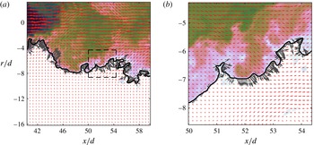
) plane. The measurement set-up described here is used for the entrainment velocity analysis discussed in this paper. A two-camera set-up was implemented for the PIV measurements. A large field of view (LFOV) region of flow was captured with one camera, whilst a small field of view (SFOV) focusing on the region around the TNTI was captured by the second camera. The measurement regions of the PIV cameras are illustrated in figure 5 (also see figure 2). To track the evolution of the TNTI in time, simultaneous PLIF measurements were performed using rhodamine 6G (Sigma-Aldrich Co. LLC) as the passive dye; this dye exhibits maximum light absorptivity at 525 nm and maximum light emissivity at 555 nm (Crimaldi Reference Crimaldi2008). The molecular diffusivity rate of rhodamine 6G is
 $1.2\times 10^{-10}~\text{m}^{2}~\text{s}^{-1}$
and the Schmidt number of the scalar field is
 $Sc=8000$
. Although the Batchelor scale,
 $\unicode[STIX]{x1D702}_{B}=1.1~\unicode[STIX]{x03BC}\text{m}$
, is too small to capture, we are primarily interested in the scaling of the mass flux across the inertial range rather than resolving the fluxes at the very smallest scalar scales. This is reflected in the fact that we apply spatial filters to the velocity and scalar data.
(a) The instantaneous scalar concentration field, shown in logarithmic scaling in the background, with the TNTI denoted by the black line. The instantaneous velocity vectors from the LFOV PIV camera are superimposed onto the figure in red; only every fourth velocity vector is shown for clarity. Along the TNTI we plot the local entrainment velocity,
 $v_{n}$
, in grey. The length of the grey
 $v_{n}$
vectors and the red velocity vectors are scaled differently. The box (black dashed lines) indicates the spatial extents of the higher-resolution PIV. (b) As in (a) but for the higher-resolution SFOV PIV camera.

For the PIV measurements the flow was seeded with
 $10~\unicode[STIX]{x03BC}\text{m}$
silver-coated, hollow glass sphere particles (Dantec Dynamics A/S). A single high-speed 527 nm Nd:YLF laser (Quantronix Darwin Duo) illuminated both the particles and dye. The laser beam was passed through a series of beam-collimating spherical optics (Thorlabs Inc.) before passing through plano-concave cylindrical lenses to form a light sheet of thickness 1.5 mm. The laser-sheet thickness was selected to approximately match the in-plane resolution of the PIV. Notch filters were placed in front of the
 $1024\times 1024$
pixel high-speed cameras (Photron SA1.1) to separate the PLIF signal from the intensity field produced by Mie scattering of particles for the PIV measurement. The velocity and scalar fields were recorded at 1 kHz, which gives a vector/scalar field spacing (1 ms) that captures the smallest temporal evolutions of the flow as determined by the Kolmogorov time scale,
 $\unicode[STIX]{x1D70F}=10.7~\text{ms}$
. Each experimental run consisted of 5457 sequential images that generate 5454 time-resolved velocity and scalar fields; six runs were performed to yield a total of
 $32\,724$
vector/scalar fields. The use of a high-repetition laser also allowed us to optimise the particle-image separation times independently for the LFOV PIV (
 $\unicode[STIX]{x1D6FF}t=3~\text{ms}$
) and SFOV PIV (
 $\unicode[STIX]{x1D6FF}t=2~\text{ms}$
) measurements. PIV processing was performed using DaVis 8.2.2 (LaVision GmbH). We implemented multi-pass processing in which the interrogation windows are shifted and deformed as per the previous cross-correlation pass. The initial particle-image correlations were performed with
 $64\times 64~\text{px}^{2}$
interrogation windows, followed by
 $32\times 32~\text{px}^{2}$
windows for the SFOV PIV, and then
 $24\times 24~\text{px}^{2}$
for the LFOV PIV.
The scalar concentration data were captured by each pixel of the PLIF camera sensor to give
 $1024\times 1024$
points of data across the FOV. It is necessary to downsample this data to match the vector spacing of the LFOV and SFOV for analysis of scalar fluxes. Alternatively, it is possible to interpolate the velocity field onto the same grid as the scalar field. However, this would become computationally expensive and would require impractical amounts of computer memory (Aanen Reference Aanen2002). To downsample the scalar images we first apply a low-pass second-order Butterworth filter to eliminate wavenumber fluctuations that are larger than the spatial resolution of the PIV fields. The low-pass filter technique has the added advantage of more effectively removing the random, high-frequency camera noise from the scalar images. The filtered scalar fields are then interpolated (bilinear interpolation) onto a grid that matches the PIV measurements.
An example of the data captured with the set-up described here is presented in figure 5. The use of this multi-scale experimental set-up makes possible the measurement of a large dynamic range from the small scales (SFOV) to the integral length scales (LFOV) of the flow. In combination with PLIF, we simultaneously measure the scalar field that is used to identify the TNTI. Details of the measurement resolution and data-set description are given in table 1. From the
 $32\,724$
vector and scalar fields we extract 1080 equally spaced fields with which we calculate the results presented in § 4.
2.4 Identification and some characteristics of the turbulent/non-turbulent interface
Isosurfaces of vorticity are commonly used in DNS and particle-tracking experiments to identify the TNTI (Holzner et al.
Reference Holzner, Liberzon, Nikitin, Kinzelbach and Tsinober2007; da Silva & Pereira Reference da Silva and Pereira2008; Wolf et al.
Reference Wolf, Lüthi, Holzner, Krug, Kinzelbach and Tsinober2012; van Reeuwijk & Holzner Reference van Reeuwijk and Holzner2014). However, a surrogate marker for the turbulent region is required for planar measurements that only capture one component of vorticity. We use isocontours of the scalar concentration field,
 $\unicode[STIX]{x1D719}$
, to identify the TNTI. This marker has been used previously in a mixing layer DNS by Sandham et al. (Reference Sandham, Mungal, Broadwell and Reynolds1988) and in planar experiments on a jet by Westerweel et al. (Reference Westerweel, Fukushima, Pedersen and Hunt2009). The scalar concentration field (
 $Sc=1$
) has also been shown to agree very well with the 3D vorticity field by Gampert et al. (Reference Gampert, Boschung, Hennig, Gauding and Peters2014) in the DNS of a temporal mixing layer. Following these researchers, we identify the TNTI by applying a threshold to the scalar concentration field that has been normalised by the local mean centreline concentration value,
 $\unicode[STIX]{x1D719}/\unicode[STIX]{x1D719}_{c}$
. An empirical process is used to identify the threshold value that best represents the TNTI. This is achieved by evaluating the area-averaged values of four variables across all the points inside the region where the local scalar concentration is larger than the given threshold value,
 $\unicode[STIX]{x1D719}>\unicode[STIX]{x1D719}_{t}$
. For a given variable,
 $f$
, the conditional average at threshold
 $\unicode[STIX]{x1D719}_{t}$
is defined as
 $$\begin{eqnarray}\tilde{f}(\unicode[STIX]{x1D719}_{t})=\frac{\displaystyle \int (f\,\text{d}a)|_{\unicode[STIX]{x1D719}>\unicode[STIX]{x1D719}_{t}}}{\displaystyle \int \text{d}a|_{\unicode[STIX]{x1D719}>\unicode[STIX]{x1D719}_{t}}}.\end{eqnarray}$$
Evidently, any such quantity will be a function of
 $\unicode[STIX]{x1D719}_{t}$
, and we look for a distinct change in such quantities as
 $\unicode[STIX]{x1D719}_{t}$
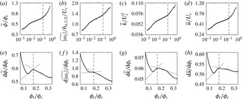
is varied. Similar techniques have been suggested by Prasad & Sreenivasan (Reference Prasad and Sreenivasan1989) and Westerweel et al. (Reference Westerweel, Hofmann, Fukushima and Hunt2002) for identifying the TNTI using scalar fields. The variables that we measure are: (i) scalar concentration,
 $\unicode[STIX]{x1D719}/\unicode[STIX]{x1D719}_{c}$
, (ii) spanwise vorticity magnitude,
 $|\unicode[STIX]{x1D714}_{z}|$
, (iii) turbulence kinetic energy,
 $k$
, and (iv) streamwise velocity,
 $u$
. Area-averaged distributions of these quantities are presented in figure 6(a–d). Points that exceed the scalar concentration threshold but exist outside of the primary scalar region (i.e. islands of scalar concentration present in the ambient fluid region) are not included in the calculation of the conditional averages. Points that are less than the scalar concentration threshold but exist within the primary scalar region (i.e. holes in the turbulent region) are included in the calculation of the conditional averages. That
 $\tilde{\unicode[STIX]{x1D719}}$
is much larger than the scalar threshold,
 $\unicode[STIX]{x1D719}_{t}$
, in figure 6(a) is to be expected because the area average includes the turbulent region, for which the scalar concentration is typically
 $O(\unicode[STIX]{x1D719}_{c})$
; see also Westerweel et al. (Reference Westerweel, Hofmann, Fukushima and Hunt2002) and their figure 4.
(a) Mean scalar concentration
 $\widetilde{\unicode[STIX]{x1D719}}$
conditioned on points over the whole domain that satisfy
 $\unicode[STIX]{x1D719}>\unicode[STIX]{x1D719}_{t}$
, where
 $\unicode[STIX]{x1D719}_{t}$
is a given scalar threshold value. (b) Conditional mean spanwise vorticity magnitude
 $\widetilde{|\unicode[STIX]{x1D714}_{z}|}$
. (c) Conditional mean turbulent kinetic energy
 $\widetilde{k}$
. (d) Conditional mean axial velocity
 $\widetilde{u}$
. Plots (a–d) are presented with logarithmic scaling. Plots (e–h) represent the derivative
 $\text{d}\widetilde{f}/\text{d}\unicode[STIX]{x1D719}_{t}$
of the conditional profiles in plots (a–d). The derivative profiles are presented with linear scaling.

We identify the interface between the turbulent and non-turbulent regions by determining the scalar threshold that coincides with the inflection points of the conditional mean value profiles in figure 6(a–d); this process has similarities to that described by Prasad & Sreenivasan (Reference Prasad and Sreenivasan1989). We identify each inflection point by considering the derivative of the conditional profiles,
 $\text{d}\tilde{f}/\text{d}\unicode[STIX]{x1D719}_{t}$
, which is shown in figure 6(e–h). The scalar concentration, spanwise vorticity and axial velocity exhibit inflection points at
 $\unicode[STIX]{x1D719}_{t}/\unicode[STIX]{x1D719}_{c}=0.18$
. The turbulence kinetic energy,
 $k$
, field exhibits an inflection point at a lower threshold (
 $\unicode[STIX]{x1D719}_{t}/\unicode[STIX]{x1D719}_{c}=0.17$
). This may be attributed to the presence of irrotational fluctuations in the non-turbulent region of the flow. We therefore use the inflection point of the scalar concentration, spanwise vorticity and velocity fields to identify the TNTI, for which
 $\unicode[STIX]{x1D719}_{t}/\unicode[STIX]{x1D719}_{c}=0.18$
. This scalar threshold is applied to each centreline-normalised, instantaneous scalar concentration field. The TNTI is extracted by applying the contour function in Matlab (MathWorks) and selecting the longest continuous isocontour. ‘Islands’ of scalar concentration that exist outside of the turbulent region and ‘holes’ of un-dyed fluid inside the turbulent region are excluded from analysis pertaining to the TNTI. The justification for this is presented later in this section.
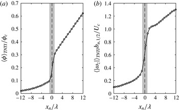
Conditionally averaged profiles of (a) scalar concentration,
 $\unicode[STIX]{x1D719}$
, and (b) spanwise vorticity magnitude,
 $|\unicode[STIX]{x1D714}_{z}|$
, along an axis that is locally normal to the TNTI. The narrow region over which a jump in the scalar concentration profile occurs is denoted by the vertical grey bar (
 $x_{n}\pm \unicode[STIX]{x1D706}$
).

The conditionally averaged profiles (denoted by
 $\langle {\sim}\rangle _{TNTI}$
) presented in figure 7 confirms that the
 $Sc\gg 1$
passive scalar successfully demarcates the turbulent region of the flow. In this figure we present the conditionally averaged profiles profiles of
 $\unicode[STIX]{x1D719}$
and
 $|\unicode[STIX]{x1D714}_{z}|$
that are calculated along coordinates that are locally normal to the TNTI,
 $x_{n}$
. In some instances
 $x_{n}$
crosses another point along the TNTI; this results in another transition from turbulent to non-turbulent fluid or vice versa. Points beyond any secondary crossings of the TNTI are excluded from the conditional average. In figure 7 we observe a jump in the scalar concentration profile across the TNTI,
 $x_{n}=0$
. The region over which the scalar concentration jump occurs, denoted by the vertical grey bars, is approximately
 $2\unicode[STIX]{x1D706}$
. However, this measured thickness is strongly influenced by spatial resolution; resolution of the order of the Batchelor scale is required to recover the true scalar gradient across the TNTI. More importantly, however, we observe that the spanwise vorticity profile in figure 7(b) exhibits a jump that coincides with the jump in scalar concentration. The spanwise vorticity magnitude is non-zero in the non-turbulent region (
 $x_{n}<0$
) due to particle displacement measurement error in PIV (Westerweel et al.
Reference Westerweel, Fukushima, Pedersen and Hunt2009). In any case, the fact that the spanwise vorticity exhibits a steep jump across the isocontours that are defined from the scalar concentration field indicates that a
 $Sc\gg 1$
passive scalar is a reliable marker of the turbulent region in the jet flow discussed here. In other words, the passive dye is not decoupled from the vorticity field. The TNTI is a region of finite thickness across which the vorticity smoothly transitions from the non-turbulent levels to the magnitude of the turbulent region (Taveira & da Silva Reference Taveira and da Silva2014; Chauhan et al.
Reference Chauhan, Philip and Marusic2014a
). Therefore, the scalar threshold that we identify (
 $\unicode[STIX]{x1D719}/\unicode[STIX]{x1D719}_{c}=0.18$
) falls within the finite thickness of the TNTI, as given by the sharp transition in spanwise vorticity in figure 7(b).
One of the consequences of the self-similarity of the flow is that the distribution of the TNTI radial position,
 $r_{I}$
, is also self-similar (Bisset et al.
Reference Bisset, Hunt and Rogers2002; Westerweel et al.
Reference Westerweel, Fukushima, Pedersen and Hunt2005; Gampert et al.
Reference Gampert, Boschung, Hennig, Gauding and Peters2014; Chauhan et al.
Reference Chauhan, Philip, de Silva, Hutchins and Marusic2014b
). Here, the subscript
 $I$
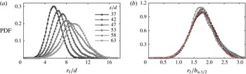
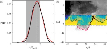
denotes values along the interface. The self-similarity of the TNTI radial position is confirmed in figure 8, in which we present (a) the PDFs of the radial position of the TNTI across short streamwise spans of the flow, and (b) the PDFs of the radial position normalised by the local jet half-width. The normalised PDF profiles in figure 8(b) are approximately Gaussian (red dashed line) and exhibit good collapse over
 $30d$
of streamwise extent. Moreover, the mean radial position of the TNTI scales linearly with streamwise distance, as shown in figure 4(c). The TNTI is much wider than the usual measures of the
 $\text{e}^{-1}$
and half-widths of jets, which suggests these latter spatial locations (
 $b_{u,\text{e}^{-1}}$
and
 $b_{u,1/2}$
) remain in the turbulent region.
(a) PDFs of the TNTI radial position,
 $r_{I}$
, for short streamwise sections
 $x/d\pm 2.5$
across values shown in legend; the radial positions are normalised by the nozzle-exit diameter,
 $d$
. (b) PDFs of the TNTI radial height for same streamwise sections as (a), but the radial positions are normalised by local jet velocity half-width,
 $b_{u,1/2}$
. A Gaussian fit is shown in the dashed red line.

The planar intersection of the measurement plane with the turbulent jet yields ‘holes’ in the turbulent region and detached eddies (‘islands’) in the non-turbulent region. Without access to volumetric information, we cannot infer if the holes are engulfed parcels of irrotational fluid or if the holes are connected to the ambient region. Similarly, the detached eddies that are isolated in the non-turbulent region may be completely detached from the turbulent region or may be attached but in a different azimuthal plane. With regards to the ‘holes’, researchers have found very little irrotational fluid within the turbulent region of different shear flows (see the Introduction). Indeed, we determine that the percentage of the turbulent area that contains engulfed fluid only amounts to 0.44 %. The engulfed fluid area is determined by measuring the number of points within the turbulent region that exhibit a scalar concentration that is less than the TNTI scalar threshold of
 $\unicode[STIX]{x1D719}/\unicode[STIX]{x1D719}_{c}=0.18$
. This definition of engulfed fluid follows from the ‘scalar cut-and-connect’ description given by Sandham et al. (Reference Sandham, Mungal, Broadwell and Reynolds1988). The size of the turbulent region is given by the number of points between the centreline of the jet and the TNTI; we exclude detached eddies in the measurement of the total turbulent area. We also evaluate the area of the detached eddies in the non-turbulent region. This is determined by measuring the number of points in the non-turbulent region that exhibit a scalar concentration that is greater than the TNTI scalar threshold. The area of detached eddies amounts to 0.86 % of the turbulent area. It this paper we disregard holes in the turbulent region and detached eddies in the non-turbulent region from our analysis because these features constitute less than 1 % of the measured flow area and may be considered to have a negligible effect on the presented results. The box-counting results presented in § 4.2 neglects the ‘holes’ and ‘islands’ that are present in the instantaneous fields; only boxes that intersect the TNTI contour are counted.
2.5 Entrainment velocity: measurement technique and characterisation
The motion of the TNTI in the laboratory frame of reference is attributed to (i) the local flow field advecting the turbulence in space, and (ii) the spreading of the turbulent region due to the entrainment of non-turbulent fluid. The former represents the local fluid velocity along the TNTI and the latter represents the entrainment velocity,
 $v_{n}$
, along the TNTI. To isolate the local entrainment velocity we must subtract the effects of the local fluid velocity from the motion of the TNTI. This requires simultaneous tracking of the TNTI and measurement of the surrounding velocity field. We achieve this by implementing high-speed PLIF to identify and track the TNTI, whilst simultaneously measuring the fluid velocity using the high-speed PIV. This process is similar to the ‘graphical’ approach of Wolf et al. (Reference Wolf, Lüthi, Holzner, Krug, Kinzelbach and Tsinober2012), who employed 3D particle-tracking data in a relatively low-
 $Re\approx 5000$
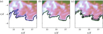
turbulent jet flow. We present a series of plots in figure 9 that illustrate the process used to calculate the local entrainment velocity. The entrainment velocity is obtained by subtracting the local fluid velocity from the net interface motion, and a description of this process is given below.
Depiction of the measurement of the local entrainment velocity,
 $v_{n}$
, using time-resolved velocity and scalar data. A description of this process is given in § 2.5. Note that the interface-normal vectors
 $\boldsymbol{n}\equiv (\unicode[STIX]{x1D735}\unicode[STIX]{x1D719}/|\unicode[STIX]{x1D735}\unicode[STIX]{x1D719}|)_{I}$
in (c) are pointing into the turbulent region.

-
(1) Consider the TNTI at two points in time: figure 9(a) shows the scalar concentration field (background contours) and the corresponding TNTI (thick black line) at an arbitrary time,
 $t_{0}$
. The TNTI at time
$t_{0}+\unicode[STIX]{x1D6FF}t$
will have moved because of the sum of the local flow advection and the local entrainment. This second interface is shown in purple, with the local fluid velocity,
$\boldsymbol{u}_{I}$
, interpolated along the interface (purple vectors).
-
(2) Subtract local advection: We subtract the effects of local advection by displacing the second interface (purple line) by distance
$-\boldsymbol{u}_{I}\unicode[STIX]{x1D6FF}t$
; the resultant shifted-interface is presented as the green line in figure 9(b). Compared with the interface at
$t_{0}+\unicode[STIX]{x1D6FF}t$
(purple line), the advection-subtracted interface (green line) exhibits much closer overlap with the original interface at
$t_{0}$
(black line). -
(3) Calculate normal distance: We finally calculate the local entrainment velocity by considering the local normal distance,
$\unicode[STIX]{x1D6FF}\boldsymbol{\ell }\boldsymbol{\cdot }\boldsymbol{n}$
, from the original interface (black) to the advection-subtracted interface (green):
$v_{n}=(\unicode[STIX]{x1D6FF}\boldsymbol{\ell }\boldsymbol{\cdot }\boldsymbol{n})/\unicode[STIX]{x1D6FF}t$
; see figure 9(c). The black arrows in this final plot represent the local normals along the original TNTI that are calculated by
$\boldsymbol{n}\equiv (\unicode[STIX]{x1D735}\unicode[STIX]{x1D719}/|\unicode[STIX]{x1D735}\unicode[STIX]{x1D719}|)_{I}$
. Note that the interface normals are pointing into the turbulent region.



Selecting the interface-separation time,
 $\unicode[STIX]{x1D6FF}t$
, for the entrainment velocity calculation requires an empirical approach, and depends on the data set and flow-type being considered. This approach is described in appendix A. Briefly, the measurement of the local entrainment velocity along the TNTI is affected by the random errors in the PIV and PLIF measurements, and the effects of out-of-plane motion. We implement a sensitivity analysis to determine the
 $\unicode[STIX]{x1D6FF}t$
that minimises the r.m.s.-fluctuations of
 $v_{n}$
and also exhibits a mean entrainment velocity that is insensitive to changes in
 $\unicode[STIX]{x1D6FF}t$
. The combination of these two criteria minimises the errors of the entrainment velocity calculation. From this approach we select
 $\unicode[STIX]{x1D6FF}t/\unicode[STIX]{x1D70F}=1.68$
for the LFOV data and
 $\unicode[STIX]{x1D6FF}t/\unicode[STIX]{x1D70F}=0.65$
for the SFOV data; these interface-separation times are used across all filter sizes,
 $\unicode[STIX]{x1D6E5}$
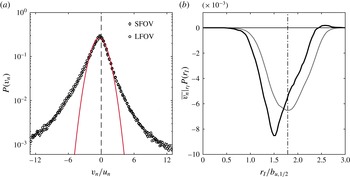
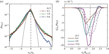
(the filtering analysis is explained further in § 4.1). That this method does indeed accurately capture the local entrainment velocity is supported by the PDF of entrainment velocity,
 $P(v_{n})$
, presented in figure 10(a). The distribution of
 $v_{n}$
is qualitatively in very good agreement with the PDFs from 3D measurements by Holzner & Lüthi (Reference Holzner and Lüthi2011), Wolf et al. (Reference Wolf, Lüthi, Holzner, Krug, Kinzelbach and Tsinober2012), and Krug et al. (Reference Krug, Holzner, Lüthi, Wolf, Kinzelbach and Tsinober2015). The negative skewness of the PDF indicates the preference for the outward growth of turbulence into the non-turbulent region, which is as expected for a turbulent jet. Furthermore, the distribution of
 $v_{n}$
is non-Gaussian, as evidenced by the wide tail of the PDF in comparison with the Gaussian distributions shown by the red line in figure 10(a).
Notice that, in order to understand
 $V_{n}$
in (1.1), we must explore the relationship between
 $v_{n}$
and
 $r_{I}$
, or more specifically how
 $v_{n}$
changes depending on the distance at which the TNTI is located. We clarify this using the conditionally averaged value of
 $v_{n}$
on
 $r_{I}$
,
 $\overline{v_{n}}|_{r_{I}}$
. If we denote
 $P(v_{n},r_{I})$
as the joint PDF of
 $v_{n}$
and
 $r_{I}$
, and
 $P(r_{I})$
as the PDF of
 $r_{I}$
, from the well-known result,
 $P(v_{n}|_{r_{I}})~P(r_{I})=P(v_{n},r_{I})$
(e.g. Papoulis Reference Papoulis1991):
 $$\begin{eqnarray}\overline{v_{n}}|_{r_{I}}P(r_{I})=\int v_{n}\,P(v_{n},r_{I})\,\text{d}v_{n}.\end{eqnarray}$$
Evidently, the left-hand side of (2.3) is only a function of
 $r_{I}$
, and represents the average value of
 $v_{n}$
at a given
 $r_{I}$
. Integrating (2.3) over all possible values of
 $r_{I}$
will result in the ensemble average value of
 $v_{n}$
along the TNTI,
 $\overline{v_{n}}^{TNTI}$
. The dark (black) line in figure 10(b) shows the left-hand side of (2.3), the area under which is equal to
 $\overline{v_{n}}^{TNTI}$
. Recall that negative
 $v_{n}$
implies that fluid is being entrained into the turbulent region. The vertical dashed–dotted line shows the average radial position of the TNTI, or
 $\int P(r_{I})\,\text{d}r_{I}$
. It is clear that most of the entrainment is occurring at a radial location that is closer to the jet centreline than the mean position, and we also observe slight ‘detrainment’ (positive
 $v_{n}$
) far from the jet centreline. This undoubtedly shows a strong dependence of
 $v_{n}$
on
 $r_{I}$
. In fact, if we assume (incorrectly) that
 $v_{n}$
and
 $r_{I}$
are independent, i.e.
 $P(v_{n},r_{I})=P(v_{n})P(r_{I})$
, then the right-hand side of (2.3) reduces to
 $\overline{v_{n}}^{TNTI}P(r_{I})$
. This quantitatively is shown in figure 10(b) by the light (grey) line, and by comparing it with the dark line visually illustrates the dependence of
 $v_{n}$
on
 $r_{I}$
.
Characteristics of the entrainment velocity (
 $v_{n}$
) along the TNTI. (a) PDF of
 $v_{n}$
,
 $P(v_{n})$
, including both the SFOV (♢) and LFOV (○) measurements. A Gaussian distribution (red line) is superimposed on the PDF. (b) The entrainment velocity conditioned on the radial location of the TNTI (
 $r_{I}$
),
 $\overline{v_{n}}|_{r_{I}}P(r_{I})$
(dark line). The light (grey) line represents
 $\overline{v_{n}}^{TNTI}P(r_{I})$
.

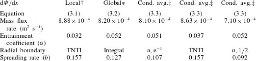
Comparison of the mass-flux rates using the local and global entrainment definitions.
 $\dagger$
Mass-flux rate is directly obtained by the knowledge of the local entrainment velocity (
 $v_{n}$
) and integrating it over the filtered TNTI (
 $\unicode[STIX]{x1D6E5}=15.6\unicode[STIX]{x1D706}$
) using (3.1);
 $\unicode[STIX]{x1D6FC}$
is calculated from
 $\unicode[STIX]{x1D6FC}=V_{n}/U_{c}$
, where
 $V_{n}$
is defined by (1.1).
 $\ast$
After calculating the mass-flux rate from (3.2) using the mean streamwise velocity,
 $\unicode[STIX]{x1D6FC}$
is obtained from (3.3) and the measured spreading rate,
 $b_{u,\text{e}^{-1}}$
. The integral radial boundary,
 $b_{m}$
, is determined from the expression
 $b_{m}=Q/\sqrt{M}$
; these symbols are defined in appendix B.
 $\ddagger$
For these cases, the entrainment coefficient,
 $\unicode[STIX]{x1D6FC}=\unicode[STIX]{x0394}v/U_{c}$
, is directly obtained from the conditional radial velocity profiles in figure 11, which is then used in conjunction with the relevant spreading rate,
 $b$
(figure 4), to calculate the corresponding mass-flux rates.

3 Measurement of the local and global mass fluxes
This section introduces different methods of estimating the mass-flux rate,
 $\text{d}\unicode[STIX]{x1D6F7}/\text{d}x$
, to characterise the spreading of the jet. The purpose of this section is to compare interpretations of the mass-flux rate in a broader context. We present definitions for (1) the local mass-flux rate, (2) the global integral mass-flux rate, and (3) the mass-flux estimates from the global entrainment hypothesis. Furthermore, in § 3.1 we employ an unconventional technique that calculates the entrained mass-flux rate based on a velocity distribution conditioned on the TNTI. This procedure provides a unique view of mean entrainment based on the average TNTI location. Note that ascertaining the agreement between the numerical values for the local and global mass-flux rates is crucial before proceeding with any multi-scale measurement procedure. In fact, calculation of global and local mass-flux rates is the first step towards checking the validity of (1.2).
-
(1) The local mass-flux rate represents the instantaneous flux that occurs along the TNTI. In three dimensions, this would represent the product of the local entrainment velocity and the TNTI surface area (1.2). The local 2D mass-flux rate is similarly evaluated by integrating the entrainment velocity,
$v_{n}$
, along a planar intersection with the TNTI, (3.1)In this expression
$$\begin{eqnarray}\frac{\text{d}\unicode[STIX]{x1D6F7}}{\text{d}x}^{loc}=\overline{\frac{1}{L_{x}}\int _{0}^{L_{s}}(-v_{n})r_{I}\,\text{d}s}.\end{eqnarray}$$
$L_{x}$
is the streamwise extent of the measured TNTI,
$L_{s}$
is the length of the instantaneous TNTI, and
$s$
is the coordinate along the TNTI. The negative sign is added to the entrainment velocity because positive entrainment (i.e. a growing turbulent region) corresponds to negative
$v_{n}$
, since the orientation of the interface-normal,
$\boldsymbol{n}$
, points towards the turbulent region. Recall that the overline indicates ensemble average over all the different realisations. The results for the local mass-flux rate are presented in § 4 and summarised in table 2 under
$\text{d}\unicode[STIX]{x1D6F7}/\text{d}x$
: local.
-
(2) The global integral 2D flux rate is evaluated using a modified form of the mass-flux rate integral for a round jet that was presented in (2.1),
(3.2)where
$$\begin{eqnarray}\frac{\text{d}\unicode[STIX]{x1D6F7}}{\text{d}x}^{glob}=\frac{\text{d}}{\text{d}x}\left(\int _{0}^{\infty }\overline{u}r\,\text{d}r\right),\end{eqnarray}$$
$\overline{u}$
is the time-averaged axial velocity. Data from separate flow-characteri sation experiments, presented in figure 3(a), provide
$\overline{u}$
, from which we determine
$(\text{d}\unicode[STIX]{x1D6F7}/\text{d}x)^{glob}=8.20\times 10^{-4}~\text{m}^{2}~\text{s}^{-1}$
for the jet flow discussed here. For reference, we provide the integral (top-hat) width in table 2 that is defined as
$b_{m}=Q/\sqrt{M}$
(see figure 4
c).
-
(3) An alternative global 2D mass-flux rate is evaluated using the entrainment hypothesis described in Morton et al. (Reference Morton, Taylor and Turner1956) and Turner (Reference Turner1986). The modified entrainment hypothesis for the 2D mass-flux rate is
(3.3)where
$$\begin{eqnarray}\frac{\text{d}\unicode[STIX]{x1D6F7}}{\text{d}x}^{entr}=b(x)\unicode[STIX]{x1D6FC}U_{c}(x),\end{eqnarray}$$
$b(x)$
is a streamwise-dependent jet width and
$\unicode[STIX]{x1D6FC}$
is the entrainment coefficient.





Early studies of entrainment, often undertaken using single-point measurements, calculated
 $\unicode[STIX]{x1D6FC}$
in (3.3) by using the mass-flux rate from (3.2) and the measured profiles of
 $b_{u,\text{e}^{-1}}(x)$
and
 $U_{c}(x)$
. Using the scaling rates for the jet flow that are presented in figure 4,
 $b_{u,\text{e}^{-1}}=0.107(x-x_{0})$
and
 $U_{c}=5.87U_{e}d(x-x_{0})^{-1}$
, we measure an entrainment coefficient of
 $\unicode[STIX]{x1D6FC}=0.052$
. This value is in good agreement with Fischer et al. (Reference Fischer, List, Koh, Imberger and Brooks1979, p. 371), who report
 $\unicode[STIX]{x1D6FC}=0.0535$
for round jets, and also falls within the range
 $\unicode[STIX]{x1D6FC}=0.05{-}0.08$
reported by Carazzo, Kaminski & Tait (Reference Carazzo, Kaminski and Tait2006).
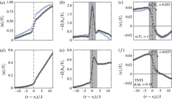
(a–c) Mean profiles conditioned on radial distance from isocontours of
 $u/U_{c}=\text{e}^{-1}$
(black circles) and
 $u/U_{c}=0.5$
(light blue squares). (d–f) As above, but conditioned on radial distance from the TNTI (isocontours of
 $\unicode[STIX]{x1D719}/\unicode[STIX]{x1D719}_{c}=0.18$
). (a,d) Conditionally averaged axial velocity profile, (b,e) mean vorticity profile given by
 $\unicode[STIX]{x1D6FA}_{z}=\unicode[STIX]{x2202}\langle u\rangle /\unicode[STIX]{x2202}r$
, (c,f) conditionally averaged radial velocity profile.

We now introduce a more representative derivation of the entrainment coefficient based on the definition that the entrainment velocity is the rate ‘at which external fluid flows into the turbulent flow across its boundary’ (Turner Reference Turner1986). This is achieved by directly measuring the velocity at which non-turbulent fluid flows into the turbulent region, in a manner similar to Chauhan et al. (Reference Chauhan, Philip, de Silva, Hutchins and Marusic2014b ); a description of this process follows.
3.1 Entrainment calculations based on conditional mean velocity distributions
Applications of the entrainment hypothesis commonly use the
 $\text{e}^{-1}$
-width (based on velocity) as a characteristic jet width. In this section we evaluate the conditionally averaged velocity distributions about instantaneous
 $\text{e}^{-1}$
-isocontours. Consider a planar, instantaneous snapshot of the axial velocity field in the far-field region of a jet where the axial velocity along radial planes is normalised by the local mean centreline velocity. We may identify a contour along the points that satisfy
 $u/U_{c}=\text{e}^{-1}$
, similar to the way we measure the TNTI. We then apply conditional averaging in a manner similar to Westerweel et al. (Reference Westerweel, Hofmann, Fukushima and Hunt2002) to evaluate the fluid behaviour on either side of the contour, although in the immediate vicinity of the
 $\text{e}^{-1}$
-contours the flow on both sides are turbulent. To do this we measure the longest contour along
 $u/U_{c}=\text{e}^{-1}$
and select the outermost points along the contour such that the contour does not come back on itself (i.e. the streamwise coordinates along the contour are monotonic). Points along the radial coordinate,
 $r$
, from the contour are extracted for each instantaneous field and normalised using local mean quantities, such as the mean centreline velocity and jet half-width. These instantaneous profiles are finally averaged to generate conditionally averaged profiles along radial coordinates from the
 $\text{e}^{-1}$
-isocontours. The resultant profiles for the axial velocity, mean vorticity, and radial velocity are presented in figure 11(a–c) (black circles).
Along isocontours of
 $u/U_{c}=\text{e}^{-1}$
we observe the presence of a strong shear layer, as illustrated by the jump in axial velocity in figure 11(a). Internal shear layers have also been reported in turbulent boundary layers by Adrian, Meinhart & Tomkins (Reference Adrian, Meinhart and Tomkins2000) and Eisma et al. (Reference Eisma, Westerweel, Ooms and Elsinga2015), and in isotropic turbulence by Hunt, Eames & Westerweel (Reference Hunt, Eames and Westerweel2014). We determine the width of this shear layer by calculating the mean vorticity profile,
 $\unicode[STIX]{x1D6FA}_{z}=\unicode[STIX]{x2202}\langle u\rangle /\unicode[STIX]{x2202}r$
, in figure 11(b) and measuring the distance across the vorticity peak. The shear layer width is defined as the distance to and from where the peak starts to appear on either side of
 $(r-r_{I})=0$
, as highlighted by the grey region. We are interested in the rate of radial inflow across this shear layer, which represents an alternative definition of the entrainment velocity. The radial velocity jump measured in figure 11(c) is determined to be
 $\unicode[STIX]{x0394}v=0.051U_{c}$
. Thus, direct measurement of the radial inflow across the
 $u/U_{c}=\text{e}^{-1}$
boundary in the turbulent jet gives an entrainment coefficient
 $\unicode[STIX]{x1D6FC}=0.051$
. Note that this value is consistent with the entrainment coefficient measured from mean-flow quantities and (3.3) (
 $\unicode[STIX]{x1D6FC}=0.052$
) and also the published values of Fischer et al. (Reference Fischer, List, Koh, Imberger and Brooks1979) (
 $\unicode[STIX]{x1D6FC}=0.0535$
). Using the entrainment coefficient measured from the conditional velocity profile and (3.3), we determine a 2D mass-flux rate of
 $(\text{d}\unicode[STIX]{x1D6F7}/\text{d}x)^{entr}=8.10\times 10^{-4}~\text{m}^{2}~\text{s}^{-1}$
, which is in very good agreement with
 $(\text{d}\unicode[STIX]{x1D6F7}/\text{d}x)^{glob}$
that is measured using (3.2).
An alternative means of applying the entrainment hypothesis is to consider the jet width defined by the TNTI,
 $b_{TNTI}$
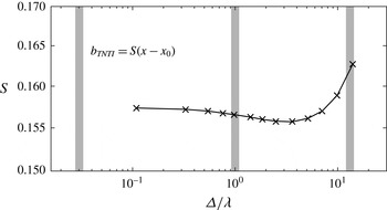
. We follow the above-described conditional averaging procedure to determine the radial inflow velocity across the TNTI; this is presented in figure 11(d–f). The measured entrainment coefficient for the TNTI in figure 11(f) is determined to be
 $\unicode[STIX]{x1D6FC}=0.037$
. Combining this coefficient with the spreading rate of the TNTI (
 $b_{TNTI}=0.157(x-x_{0})$
, figure 4
c) and (3.3) we measure a 2D mass-flux rate of
 $(\text{d}\unicode[STIX]{x1D6F7}/\text{d}x)^{entr}=8.63\times 10^{-4}~\text{m}^{2}~\text{s}^{-1}$
.
For comparison, we also determine the 2D mass-flux rate using the velocity half-width contours. Equation (3.3) is applied to the velocity half-width of the jet, where
 $b_{u,1/2}~=~0.092(x-x_{0})$
, and
 $\unicode[STIX]{x1D6FC}=0.052$
is determined using the same process as above from the conditional radial velocity profile in figure 11(c). This combination gives a mass-flux rate of
 $(\text{d}\unicode[STIX]{x1D6F7}/\text{d}x)^{entr}=7.10\times 10^{-4}~\text{m}^{2}~\text{s}^{-1}$
.
Results for mass-flux rates and entrainment coefficients using different methods are summarised in table 2. The mass-flux rates determined from these different methods are reasonably close to each other, except for the last column (
 $b_{u,1/2}$
), which is understandably lower because the average location of the half-width is far inside the turbulent region (see figure 4
c). It is also worth noting that
 $\unicode[STIX]{x1D6FC}$
from both the local and conditionally averaged methods for the TNTI are similar (
 $\unicode[STIX]{x1D6FC}\approx 0.03$
), which is lower than the usual value of
 $\unicode[STIX]{x1D6FC}\approx 0.05$
because the
 $\text{e}^{-1}$
-contour is interior to the TNTI. Recently, there have been applications of kinetic energy and momentum conservation equations to understand the physical components of the entrainment coefficient (e.g. Kaminski, Tait & Carazzo Reference Kaminski, Tait and Carazzo2005, Craske & van Reeuwijk Reference Craske and van Reeuwijk2015) following the seminal work of Priestley & Ball (Reference Priestley and Ball1955). In appendix B we apply this approach for evaluating
 $\unicode[STIX]{x1D6FC}$
to the extent made possible from the present experimental data.
4 Multi-scale entrainment results
In this section we investigate the scaling of the TNTI surface area, or in our case of 2D fields the TNTI length (
 $L_{s}$
), the mass-flux rate (
 $\text{d}\unicode[STIX]{x1D6F7}/\text{d}x$
), and the entrainment velocity (
 $V_{n}$
) as functions of the filter size (
 $\unicode[STIX]{x1D6E5}$
). The main aims of this section are to demonstrate that (i) TNTI surface area exhibits a power-law scaling (
 $S\sim \unicode[STIX]{x1D6E5}^{-D}$
), (ii) the local mass-flux rate is independent of scale (
 $\text{d}\unicode[STIX]{x1D6F7}^{loc}/\text{d}x=\text{d}\unicode[STIX]{x1D6F7}^{\unicode[STIX]{x1D6E5}}/\text{d}x=\text{d}\unicode[STIX]{x1D6F7}^{glob}/\text{d}x$
), and (iii) the entrainment velocity scales at a rate that is the inverse of the TNTI length scaling (
 $V_{n}\sim \unicode[STIX]{x1D6E5}^{D}$
). First, we introduce the spatial-filtering techniques that are implemented in this study. We then present our results on the scaling of the TNTI length with the use of a box-counting technique and a spatial-filtering technique. The multi-scale FOV correction is then discussed, which is necessary for the subsequent mass-flux and entrainment velocity results.
The interface length scaling is measured using the scalar fields from the PLIF data set; these points are denoted by triangles (▵) in the figures to follow. The mass-flux rate and the entrainment velocity scaling are measured using the combined multi-scale-PIV and PLIF data sets; these points are denoted by squares (▫) for SFOV data and circles (○) for LFOV data. We also assess the sensitivity of these scaling results on the scalar threshold that identifies the TNTI by considering different scalar thresholds. We evaluate the scaling results for scalar thresholds of
 $\unicode[STIX]{x1D719}/\unicode[STIX]{x1D719}_{c}=0.14$
(light pink) and
 $\unicode[STIX]{x1D719}/\unicode[STIX]{x1D719}_{c}=0.22$
(light blue); these values are
 $\pm 20\,\%$
of the TNTI threshold (
 $\unicode[STIX]{x1D719}/\unicode[STIX]{x1D719}_{c}=0.18$
) determined in § 2.4.
4.1 Data filtering procedure
We follow the procedure of Philip et al. (Reference Philip, Meneveau, da Silva and Marusic2014) to implement a spatial-filtering technique to evaluate the entrainment scaling. The instantaneous velocity and scalar concentration fields are filtered with box-averaging filters across a range of filter sizes,
 $\unicode[STIX]{x1D6E5}$
. This is achieved with the convolution of the velocity and scalar fields with filter
 $G_{\unicode[STIX]{x1D6E5}}$
,
 $\hat{u} _{\unicode[STIX]{x1D6E5}}=u\ast G_{\unicode[STIX]{x1D6E5}}$
, where
 $$\begin{eqnarray}G_{\unicode[STIX]{x1D6E5}}(r)=\left\{\begin{array}{@{}ll@{}}0,\quad & |r|\geqslant \unicode[STIX]{x1D6E5}/2,\\ 1/\unicode[STIX]{x1D6E5}^{2},\quad & |r|<\unicode[STIX]{x1D6E5}/2.\end{array}\right.\end{eqnarray}$$
The multi-scale-PIV measurements allow for over two decades of filter size scaling from
 $\unicode[STIX]{x1D6E5}/\unicode[STIX]{x1D706}=0.11$
to
 $\unicode[STIX]{x1D6E5}/\unicode[STIX]{x1D706}=16$
. We apply the same threshold (
 $\unicode[STIX]{x1D719}/\unicode[STIX]{x1D719}_{c}=0.18$
) across all
 $\unicode[STIX]{x1D6E5}$
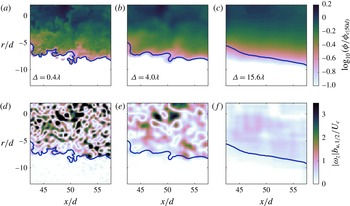
to identify the TNTI. The effects of spatial filtering are shown in figure 12, which compares instantaneous scalar concentration (a–c) and spanwise vorticity (d–f) fields, and the respective TNTI (blue lines) for different filter sizes. Figure 12(d–f) shows that the scalar interface closely encloses the spanwise vorticity field of the turbulent jet. That the scalar concentration boundary and vorticity boundary do indeed overlap is also illustrated in figure 7, in which we show that the jump in
 $\unicode[STIX]{x1D719}$
across the TNTI coincides with a jump in
 $|\unicode[STIX]{x1D714}_{z}|$
. Hence, the scalar concentration threshold chosen for this study successfully isolates the turbulent from the non-turbulent (irrotational) regions.
Comparison of three different filter lengths applied to an instantaneous scalar concentration field (a–c) and the spanwise vorticity fields
 $|\unicode[STIX]{x1D714}_{z}|$
(d–f). The TNTI is depicted by the thick blue line and is determined using the
 $\unicode[STIX]{x1D719}/\unicode[STIX]{x1D719}_{c}=0.18$
threshold. The scalar concentration fields are shown in logarithmic scaling.

4.2 Scaling of the TNTI surface area
The box-counting technique applied to turbulent surfaces is commonly used to determine the fractal dimension of a surface (e.g. Mandelbrot Reference Mandelbrot1982 and Sreenivasan & Meneveau Reference Sreenivasan and Meneveau1986). This process counts the number of boxes (
 $N$
) of side width
 $\unicode[STIX]{x1D6E5}$
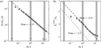
that occupy the TNTI, which is then repeated for a large range of box sizes. We apply the box-counting technique to all 1080 scalar fields, the results of which are presented in figure 13(a). The box widths span from a few Kolmogorov length scales to beyond the jet half-width. A least-squares fit applied in the range
 $0.3\unicode[STIX]{x1D706}\leqslant \unicode[STIX]{x1D6E5}\leqslant 10\unicode[STIX]{x1D706}$
determines that the TNTI exhibits a fractal dimension of
 $D_{2}=1.33$
, where
 $N\sim \unicode[STIX]{x1D6E5}^{-D_{2}}$
. This scaling of the TNTI jet agrees well with the recent fractal scaling results of surfaces in a turbulent boundary layer presented by de Silva et al. (Reference de Silva, Philip, Chauhan, Meneveau and Marusic2013), who report a fractal dimension of
 $D_{2}=1.31$
for the TNTI measured in a turbulent boundary layer. More generally, de Silva et al. (Reference de Silva, Philip, Chauhan, Meneveau and Marusic2013) report that the fractal dimension of the TNTI in a boundary layer falls within the range
 $D_{2}=1.3$
to
 $1.4$
. This is also supported by Chauhan et al. (Reference Chauhan, Philip, de Silva, Hutchins and Marusic2014b
), who report a fractal dimension of
 $D_{2}=1.3$
, and by Zubair & Catrakis (Reference Zubair and Catrakis2009), who report a fractal dimension for scalar isocontours in a shear layer flow of
 $D_{2}=1.3$
. For a planar intersection with a fractal surface, the 3D fractal dimension is given by
 $D_{3}\equiv D_{2}+1=2.33$
(see Mandelbrot Reference Mandelbrot1982), which also is in very good agreement with the theoretical analysis of Sreenivasan et al. (Reference Sreenivasan, Ramshankar and Meneveau1989) based on the Kolmogorov similarity hypothesis, where
 $D_{3}=7/3$
and is determined by assuming a Reynolds-number-independent entrainment rate. In addition, the fractal dimension does not change for the
 $\unicode[STIX]{x1D719}/\unicode[STIX]{x1D719}_{c}=0.18\pm 20\,\%$
scalar thresholds that are also considered; these data are shown in light pink and light blue. Hence, the fractal dimension is not particularly sensitive to the particular choice of threshold for the TNTI.
(a) Box counting applied to the TNTI from the full resolution scalar images. The vertical grey bars in the background indicate the Kolmogorov length scale,
 $\unicode[STIX]{x1D702}$
, the Taylor microscale,
 $\unicode[STIX]{x1D706}$
, and the jet half-width,
 $b_{u,1/2}$
, at
 $50d$
from left to right, respectively. (b) The scaling of the mean TNTI length,
 $\overline{L_{s}}^{TNTI}$
, with box-filter size,
 $\unicode[STIX]{x1D6E5}$
. The expected scaling of
 $\overline{L_{s}}^{TNTI}\sim \unicode[STIX]{x1D6E5}^{-1/3}$
is plotted as a grey dash-dotted line for comparison.

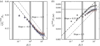
Figure 13(b) presents an alternative means of measuring the fractal dimension of a 2D boundary. A similar procedure is also applied to the TNTI in turbulent boundary layers by de Silva et al. (Reference de Silva, Philip, Chauhan, Meneveau and Marusic2013). We spatially filter each instantaneous scalar concentration field at each filter size,
 $\unicode[STIX]{x1D6E5}$
, and directly measure the corresponding mean length of the TNTI,
 $\overline{L_{s}}^{TNTI}$
. The interface length is expected to scale as
 $\overline{L_{s}}^{TNTI}\sim \unicode[STIX]{x1D6E5}^{1-D_{2}}$
, because
 $\overline{L_{s}}^{TNTI}\sim \unicode[STIX]{x1D6E5}N$
. In figure 13(b) we apply a least-squares fit between
 $0.5\unicode[STIX]{x1D706}<\unicode[STIX]{x1D6E5}<3\unicode[STIX]{x1D706}$
that measures a fractal dimension of
 $-0.31$
(
 $D_{2}=1.31$
), which is in good agreement with the box-counting technique, for which
 $D_{2}=1.33$
. The interface length scaling for
 $\unicode[STIX]{x1D719}/\unicode[STIX]{x1D719}_{c}=0.18\pm 20\,\%$
also agrees well with the TNTI data; this supports the idea that the interface length scaling is not dependent on a specific scalar threshold for the TNTI. Note that the ‘tailing-off’ effect for very small and large filter lengths in figure 13(b) is indicative of the fact that the fractal scaling ceases to exist beyond those limits. In any case, our primary interest is the scaling rate across the inertial range, for which the data exhibit almost a decade of linear scaling on the log–log plot in figure 13(b).
It is worth mentioning that
 $Sc\gg 1$
isoscalar surfaces will exhibit two distinct scaling regimes: a viscous advective regime (with a suggested fractal scaling of
 $7/3$
) that is the focus of this paper, and a diffusive viscous regime that exists between the Batchelor length scale and the Kolmogorov length scale (Sreenivasan et al.
Reference Sreenivasan, Ramshankar and Meneveau1989; Sreenivasan & Prasad Reference Sreenivasan and Prasad1989). It is expected that the diffusive viscous regime exhibits a different fractal dimension,
 $D_{B}=2.65$
, with experimental measurements suggesting
 $D_{B}\approx 2.7$
at a relatively low
 $Re=1500$
(Sreenivasan & Prasad Reference Sreenivasan and Prasad1989). The results presented in figure 13 do not exhibit the steeper power-law scaling that is expected for the latter regime. This is because the results presented in figure 13 are limited by the spatial resolution of the scalar concentration field, which is larger than the Kolmogorov length scale.
4.3 Correction for SFOV data
A compromise of the multi-scale PIV arrangement is that while the LFOV captures the full radial extent of the TNTI, the SFOV cannot, which instead focuses on a smaller region and providing higher resolution. Figure 14(a) shows a PDF of the radial position of the TNTI normalised by the local velocity half-width. The measurement area of the SFOV is represented by the greyed region. It is apparent that the SFOV PIV does not capture the entrainment that occurs when the TNTI is far from the turbulent core (
 $r_{I}/b_{u,1/2}\geqslant 2$
). In the following analysis we compare the SFOV and LFOV entrainment scaling across the same radial extent to account for any bias introduced by the TNTI moving out of the FOV. In other words, we present scaling results from the LFOV that are calculated using points that are within the radial confines of the SFOV. This data processing step is illustrated in figure 14(b), in which the spatial extent of the LFOV (full image) is compared with that for the SFOV (shown in the white dashed square). The coloured section of the plot represents the radial span in which the LFOV data are used for comparison with the SFOV data. In figure 15 (to be discussed in §§ 4.4 and 4.5), the LFOV data points that are from the limited radial extents are shown in hollow black circles whereas data measured across the full radial extent of the LFOV are shown in filled grey circles. The SFOV data are represented by the hollow black squares.
(a) PDF of the radial position of the TNTI, normalised by the local jet velocity half-width,
 $b_{u,1/2}$
; the red line represents a Gaussian fit and the dot-dashed line is the mean interface position (
 $\overline{r_{I}}^{TNTI}/b_{u,1/2}=1.79$
). The greyed region represents the radial extents of the SFOV PIV. (b) Instantaneous scalar concentration field of the LFOV with the SFOV extents shown in the white dashed line. The coloured section of the plot represents the LFOV entrainment velocity points along the TNTI (green) that are used in comparisons of the 2D flux rate and entrainment velocity with the SFOV data.

(a) The scaling of the local 2D flux rate (3.1) for the SFOV (squares) and LFOV (circles) data; the horizontal dashed line represents the global 2D flux rate (3.2). The hollow black markers indicate data measured within the radial limits shown in figure 14 and the hatched lines indicate the span of the minimum and maximum measured mass-flux rates. The filled grey markers indicate the LFOV flux rate data measured across the full radial extent of the FOV. (b) The scaling of the mean entrainment velocity,
 $V_{n}$
, normalised by the local mean centreline velocity,
 $U_{c}$
. The hatched region represents the entrainment coefficient range from figure 11(f), and (3.3) with
 $(\text{d}\unicode[STIX]{x1D6F7}/\text{d}x)^{glob}$
.

4.4 Mass-flux rate across the TNTI at multi-scales
As discussed in the introduction (see (1.2)), the theoretical analysis of Meneveau & Sreenivasan (Reference Meneveau and Sreenivasan1990) and Philip et al. (Reference Philip, Meneveau, da Silva and Marusic2014) suggests that the mass flux across the TNTI should be independent of scale. To test this hypothesis, we first filter the velocity and scalar fields and determine the TNTI from the filtered fields at different filter sizes,
 $\unicode[STIX]{x1D6E5}$
, as discussed in § 4.1. Subsequently, we calculate the entrainment velocity along the TNTI at varying filter sizes,
 $v_{n}(\unicode[STIX]{x1D6E5})$
, as detailed in § 2.5. Mass-flux rates at different length scales,
 $\text{d}\unicode[STIX]{x1D6F7}^{\unicode[STIX]{x1D6E5}}/\text{d}x$
can be found from the right-hand side of (3.1), where the different quantities are now functions of
 $\unicode[STIX]{x1D6E5}$
. Figure 15(a) shows
 $\text{d}\unicode[STIX]{x1D6F7}^{\unicode[STIX]{x1D6E5}}/\text{d}x$
as a function of
 $\unicode[STIX]{x1D6E5}$
, and it is evident that the mass flux is scale-independent. The hollow markers from the multi-scale measurements fall within the range
 $(10.78\pm 0.30)\times 10^{-4}~\text{m}^{2}~\text{s}^{-1}$
(hatched grey region) across a range of over two decades in scale. Hence, these results support the aforementioned scale-independent mass-flux hypothesis defined in (1.2). In other words, the mass flux across the contorted (long) TNTI at small scales agrees with the mass flux across the smooth (short) TNTI at large scales. The mass-flux scaling for
 $\unicode[STIX]{x1D719}/\unicode[STIX]{x1D719}_{c}=0.18\pm 20\,\%$
, shown in light pink and light blue, are also independent of filter size,
 $\unicode[STIX]{x1D6E5}$
. This further evidences that the constant mass-flux scaling result is less dependent on a specific scalar threshold.
For comparison, we also plot the global integral mass-flux rate,
 $\text{d}\unicode[STIX]{x1D6F7}^{glob}/\text{d}x=8.20\times 10^{-4}~\text{m}^{2}~\text{s}^{-1}$
(horizontal grey dashed line), which is determined using (3.2). The observed discrepancy between the local mass-flux rate (hollow black markers) and the global mass-flux rate in figure 15(a) is attributed to the bias error of the limited radial extent of the SFOV measurements. That our measurements do indeed accurately measure the turbulent entrainment is confirmed by the mass-flux rates that are determined using the full radial extent of the LFOV measurements (filled grey markers). In this case, the local mass-flux rate measured across the full FOV in figure 15(a) is in excellent agreement with the global flux rate from (3.2). Note that there is a slight increase in the mass-flux rates with filter size for
 $\unicode[STIX]{x1D6E5}>7\unicode[STIX]{x1D706}$
, which is artefact of the effect of the spatial-filtering technique on the mean radial position of the TNTI. This is discussed further in appendix C, but we simply note here that this effect does not change the fractal dimension of the scaling that we observe across the viscous advective regime.
4.5 Scaling of the entrainment velocity
In addition to the mass-flux scaling, we are also interested in evaluating the scaling of the mean entrainment velocity,
 $V_{n}$
. From (1.2), the entrainment velocity is expected to scale inversely to the TNTI surface area or length scaling. Measurement of the entrainment velocity scaling was first attempted by Philip et al. (Reference Philip, Meneveau, da Silva and Marusic2014), although they fell short in showing the scaling, primarily because of resolution issues with their experiments. Here, we evaluate the mean entrainment velocity in figure 15(b) to determine the scaling of
 $V_{n}$
along the TNTI for different filtered fields; the entrainment velocity is calculated using the integral in (1.1). Note that for each filter size,
 $\unicode[STIX]{x1D6E5}$
, the entrainment velocity is recalculated employing the procedure described in § 2.5 with the filtered PIV and PLIF data. We also normalise the entrainment velocity by the local mean centreline velocity to draw comparisons with the entrainment coefficient,
 $\unicode[STIX]{x1D6FC}$
, obtained using the entrainment hypothesis. A least-squares fit between
 $0.5\unicode[STIX]{x1D706}<\unicode[STIX]{x1D6E5}<3\unicode[STIX]{x1D706}$
determines that the entrainment velocity scales as
 $V_{n}\sim \unicode[STIX]{x1D6E5}^{0.31}$
, which is indicative of a power-law behaviour of the entrainment velocity. We exclude the outlying points consistent with the data shown in figure 13(b). Thus, within the experimental uncertainty, these results support the conclusion that the entrainment velocity scales at a rate that balances the interface length scaling,
 $\overline{L_{s}}^{TNTI}\sim \unicode[STIX]{x1D6E5}^{-0.31}$
. It is for this reason that we observe a constant mass-flux rate in figure 15(a). We anticipate that the effect of improved spatial resolution on this result would be that the measured entrainment velocity would continue to follow the black dashed line in figure 15(b) to smaller mean values of
 $V_{n}$
for smaller
 $\unicode[STIX]{x1D6E5}$
, and possibly a different slope with filter size in the viscous-diffusive regime.
Interestingly, at filter lengths of
 $\mathit{O}(10^{1}\unicode[STIX]{x1D706})$
the mean entrainment velocity from the full radial extent data (filled grey symbols) approaches the entrainment coefficient calculated in § 3 (
 $\unicode[STIX]{x1D6FC}=0.035{-}0.037$
), shown by the hatched lines in figure 15(b). The use of a large spatial filter generates a flow field that approaches the time-averaged field, which forms the basis of the global entrainment calculation (Philip et al.
Reference Philip, Meneveau, da Silva and Marusic2014). The small discrepancy between the local and global entrainment coefficients is attributed to the dependency that exists between the entrainment velocity and the radial height of the TNTI. This is illustrated by evaluating the ensemble-averaged entrainment velocity,
 $\overline{v_{n}}^{TNTI}$
, which does not take into account the dependence between
 $v_{n}$
and the radial height of the interface that exists in the mean entrainment velocity,
 $V_{n}$
(see (1.1) and figure 10). The scaling of the ensemble-averaged entrainment velocity,
 $\overline{v_{n}}^{TNTI}$
, is presented in figure 19(b) in appendix C. The magnitude of
 $\overline{v_{n}}^{TNTI}$
at a given filter size is greater than
 $V_{n}$
shown in figure 15(b). This is because the largest entrainment velocities (most negative) occur when the TNTI is closer to the jet centreline. Hence, in the expression
 $\int (-v_{n})r_{I}\,\text{d}s$
(1.1), larger (more negative) values of
 $v_{n}$
are offset by smaller values of the radial term,
 $r_{I}$
. There is much better agreement between
 $\overline{v_{n}}^{TNTI}$
for large
 $\unicode[STIX]{x1D6E5}$
(grey symbols) and the entrainment coefficient (hatched lines) if we simply consider the ensemble-averaged entrainment velocity in figure 19(b). This supports the description by Philip et al. (Reference Philip, Meneveau, da Silva and Marusic2014) in which entrainment at very large
 $\unicode[STIX]{x1D6E5}$
is completely dominated by the advective flux, which is the sole contribution to global entrainment in the RANS (time-averaged) formulation.
Effect of filtering on the characteristics of the entrainment velocity,
 $v_{n}(\unicode[STIX]{x1D6E5})$
, along the TNTI. (a) PDF of
 $v_{n}$
,
 $P(v_{n})$
. Gaussian distribution is shown by the solid grey line. (b) Entrainment velocity conditioned on the radial location of the TNTI,
 $r_{I}$
. The dashed lines represent
 $\overline{v_{n}}^{TNTI}P(r_{I})$
at different
 $\unicode[STIX]{x1D6E5}$
, similar to the light (grey) line in figure 10 for the unfiltered case. The dash-dotted line represents the mean radial location of the TNTI.

Finally, we present in figure 16 the effect of filtering on the PDF of
 $v_{n}$
and its relation to
 $r_{I}$
. This is similar to figure 10, except with a range of filter sizes. The PDF in figure 16(a) shows a reduction of mostly positive
 $v_{n}$
(detrainment) due to filtering. In figure 16(b) we present the entrainment velocity conditioned on the TNTI radial location (solid lines). The dashed lines represent
 $\overline{v_{n}}^{TNTI}P(r_{I})$
, which (incorrectly) assumes that
 $v_{n}$
and
 $r_{I}$
are independent. It is clear from this figure that the conditioned profiles (solid lines) occupy a larger area with increasing
 $\unicode[STIX]{x1D6E5}$
, corresponding to an increasing entrainment velocity. Also, with increasing filter size, figure 16(b) provides evidence of reduced
 $v_{n}$
at the farthest distances from the TNTI, and the consequent concentration of entrainment towards the mean TNTI position.
We have shown in this section that the magnitude of the entrainment velocity is scale-dependent (figure 15
b), and exhibits a power-law scaling that is the inverse of the scaling of the TNTI length, as proposed by Meneveau & Sreenivasan (Reference Meneveau and Sreenivasan1990) and Philip et al. (Reference Philip, Meneveau, da Silva and Marusic2014). At the very largest scales (
 $\unicode[STIX]{x1D6E5}\sim b_{u,1/2}$
) the mean entrainment velocity is approximately
 $(0.03{-}0.04)U_{c}$
, whereas at the smaller scales (
 $\unicode[STIX]{x1D6E5}\sim \unicode[STIX]{x1D702}$
) the mean entrainment velocity is closer to
 $0.01U_{c}$
. Consistent with the constant mass-flux rate observed in figure 15(a), we observe that the entrainment velocity is small at the smallest scales, but is balanced by the presence of a very large surface area. In the same way, the entrainment velocity is large at the largest scales, but is balanced by a smaller (smoother) surface area.
5 Summary and conclusions
We evaluated the scale dependence of the mass-flux rate and entrainment velocity across the turbulent/non-turbulent interface in an axisymmetric jet. This is achieved with time-resolved, simultaneous multi-scale-PIV/PLIF measurements taken in the far field. This novel experimental arrangement made possible the identification and tracking of the TNTI, and the measurement of the local entrainment velocity along it. The multi-scale-PIV measurements were necessary to achieve a dynamic range that measured the interface length, mass flux, and entrainment velocity across two decades of scale. The turbulent jet exhibits Reynolds numbers of
 $Re=25\,300$
and
 $Re_{\unicode[STIX]{x1D706}}=260$
, which are higher than most comparable studies of the TNTI and entrainment processes in turbulence. A large Reynolds number is necessary to achieve a distinct scale separation from the viscous scales up to the inertial scales.
Consistent with previous experimental and numerical investigations, we use the scalar concentration field of a
 $Sc\gg 1$
passive scalar to identify the TNTI. The specific scalar concentration threshold that represents the TNTI is empirically determined with the use of a conditional averaging approach. We show that there exists a jump in the spanwise vorticity magnitude across the isocontours of scalar concentration that represent the TNTI; this illustrates the effectiveness of using a
 $Sc\gg 1$
passive scalar to identify the boundary of the vorticity field. The interface-tracking technique described in § 2.5 is shown to be capable of measuring the local entrainment velocity along the TNTI. The advantage of this technique is that the local entrainment velocity, at the scale of the measurement, can be measured without requiring spatial resolution that resolves the Kolmogorov length scales of the flow. In other words, the interface-tracking technique is not resolution-dependent, which is a necessary feature in order to establish the scaling of the entrainment velocity.
A comparison is drawn between the well-established interpretation of global entrainment from an integral, entrainment hypothesis approach and the local entrainment along the TNTI. We show that the entrained mass-flux rates (
 $\text{d}\unicode[STIX]{x1D6F7}/\text{d}x$
) calculated from the local approach along the TNTI (3.1) exhibit good agreement with the mass-flux rate obtained from the global calculation (3.2). This comparison also demonstrates that the magnitude of the entrainment coefficient (
 $\unicode[STIX]{x1D6FC}$
) is dependent on the entrainment approach and the selected characteristic jet width. We also estimate the mass-flux rates using radial velocity profiles that are conditioned on the TNTI. This hybrid approach yields mass-flux rates and entrainment coefficients that agree well with the global and local methods.
The multi-scale entrainment hypothesis of Meneveau & Sreenivasan (Reference Meneveau and Sreenivasan1990) suggests that the mass-flux rate across an interface should be constant across all length scales. More concretely, this theory states that
 $$\begin{eqnarray}\frac{\text{d}\unicode[STIX]{x1D6F7}}{\text{d}x}^{loc}=\frac{\text{d}\unicode[STIX]{x1D6F7}}{\text{d}x}^{\unicode[STIX]{x1D6E5}}=\frac{\text{d}\unicode[STIX]{x1D6F7}}{\text{d}x}^{glob}=\text{const.},\end{eqnarray}$$
where the filter length scale,
 $\unicode[STIX]{x1D6E5}$
, represents any intermediate length scale. This expression is equivalent to (1.2), for which the mass-flux rate is decomposed into the scale-dependent surface area,
 $S(\unicode[STIX]{x1D6E5})$
, and entrainment velocity,
 $V_{n}(\unicode[STIX]{x1D6E5})$
. Evidence of a scale-independent mass-flux rate had not been observed in any physical scenario, primarily because of the demanding experimental and analysis techniques. These limitations are addressed in the experimental set-up and the entrainment velocity measurement technique implemented in this study. We first use two independent methods to show that the surface area,
 $S$
, exhibits a multi-scale behaviour with a fractal dimension that falls in the range
 $D_{3}\approx 2.31{-}2.33$
, where
 $S\sim \unicode[STIX]{x1D6E5}^{-D}\equiv \unicode[STIX]{x1D6E5}^{2-D_{3}}$
. More specifically, application of a box-counting technique to the TNTI yields a power-law exponent of
 $D_{2}\equiv D_{3}-1=1.33$
, and application of a spatial-filtering technique yields a power-law exponent for the TNTI length of
 $D=0.31$
, where
 $\overline{L_{s}}^{TNTI}\sim \unicode[STIX]{x1D6E5}^{-D}\equiv \unicode[STIX]{x1D6E5}^{1-D_{2}}$
. Thus, the multi-scale behaviour of the TNTI across the inertial range favours a constant power-law fractal behaviour, in agreement with de Silva et al. (Reference de Silva, Philip, Chauhan, Meneveau and Marusic2013), rather than a scale-dependent behaviour (Miller & Dimotakis Reference Miller and Dimotakis1991).
We invoke a multi-scale analysis to evaluate the scale dependence of the entrainment velocity,
 $V_{n}(\unicode[STIX]{x1D6E5})$
. We report that the entrainment velocity exhibits a power-law scaling given by
 $V_{n}\sim \unicode[STIX]{x1D6E5}^{0.31}$
. From this scaling we show that the entrainment coefficient,
 $\unicode[STIX]{x1D6FC}(\unicode[STIX]{x1D6E5})\equiv V_{n}/U_{c}$
, is also scale-dependent and ranges from
 $\unicode[STIX]{x1D6FC}\approx 0.01$
for
 $\unicode[STIX]{x1D6E5}\approx \unicode[STIX]{x1D702}$
(small scales) up to
 $\unicode[STIX]{x1D6FC}\approx 0.03{-}0.04$
for
 $\unicode[STIX]{x1D6E5}\approx b_{u,1/2}$
(large scales). Moreover, the entrainment coefficient at the largest filter size agrees well with the entrainment coefficient determined using the global (integral) definition of entrainment. The primary outcome of this study is experimental evidence that confirms that the mass-flux rate across the TNTI is independent of scale:
 $V_{n}(\unicode[STIX]{x1D6E5})S(\unicode[STIX]{x1D6E5})=\text{const.}$
This is indeed satisfied when we consider the mass-flux rate along the TNTI (5.1), and also when we consider the combined power-law behaviours of
 $V_{n}(\unicode[STIX]{x1D6E5})$
and
 $S(\unicode[STIX]{x1D6E5})$
found in our multi-scale analyses. This result suggests that the entrainment velocity scales at a rate that balances the scaling of the interface length, so as to make the net entrainment scale-independent. This result lends support to the interpretation of the roles of viscous nibbling and inviscid engulfment, in which nibbling is only active locally at the small scales, and engulfment is only active at the large scales of the flow.
Acknowledgements
The authors wish to thank the Engineering and Physical Sciences Research Council (research grant no. EP/I005897/1) and the Australian Research Council for the financial support of this work. The visit of D.M. to the University of Melbourne was supported by the David Crighton Fellowship from the Department of Applied Mathematics and Theoretical Physics, Cambridge.
Appendix A. Details of the entrainment velocity measurement: optimising
$\unicode[STIX]{x1D6FF}t$
and errors due to radial motion

A.1 Optimisation of the time delay
$\unicode[STIX]{x1D6FF}t$

We implement an empirical approach to determine the optimal interface-separation time,
 $\unicode[STIX]{x1D6FF}t$
, that minimises the errors that affect the planar measurement of the entrainment velocity. These errors are: (i) the random error of the PIV and PLIF measurement precision, and (ii) the effects of out-of-plane motion. The former error is dominant at small
 $\unicode[STIX]{x1D6FF}t$
and the latter is dominant at larger
 $\unicode[STIX]{x1D6FF}t$
. The sensitivity analysis described herein is similar to the selection process of the particle-image separation time for planar PIV, as described in Poelma, Westerweel & Ooms (Reference Poelma, Westerweel and Ooms2006).
(a) Evaluation of the r.m.s.-entrainment velocity as a function of the interface-separation time,
 $\unicode[STIX]{x1D6FF}t/\unicode[STIX]{x1D70F}$
, for the range of the coarse-graining filter lengths,
 $\unicode[STIX]{x1D6E5}$
, shown in grey markers. Filter lengths
 $\unicode[STIX]{x1D6E5}=0.4\unicode[STIX]{x1D706}$
(blue circles),
 $\unicode[STIX]{x1D6E5}=3.3\unicode[STIX]{x1D706}$
(green triangles), and
 $\unicode[STIX]{x1D6E5}=12.0\unicode[STIX]{x1D706}$
(red squares) are highlighted with filled markers. The vertical grey bars indicate interface-separation times of
 $\unicode[STIX]{x1D6FF}t/\unicode[STIX]{x1D70F}=0.09,1.68,5.61$
. (b) The ensemble-averaged entrainment velocity,
 $-\overline{v_{n}}^{TNTI}$
, as a function of
 $\unicode[STIX]{x1D6FF}t/\unicode[STIX]{x1D70F}$
.

The r.m.s.-entrainment velocity,
 $\overline{{{v_{n}}^{\prime }}^{2}}_{TNTI}^{1/2}$
, is sensitive to increases in spurious vectors that arise from the aforementioned errors. The profile of
 $\overline{{{v_{n}}^{\prime }}^{2}}_{TNTI}^{1/2}$
as a function of
 $\unicode[STIX]{x1D6FF}t$
is presented in figure 17(a) for a range of filter sizes (see § 4.1) for the LFOV set-up. First, consider the shortest filter length (
 $\unicode[STIX]{x1D6E5}=0.4\unicode[STIX]{x1D706}$
), which is represented by the filled blue circles. In the region
 $\unicode[STIX]{x1D6FF}t/\unicode[STIX]{x1D70F}<1.68$
the r.m.s.-entrainment velocity decreases with increasing
 $\unicode[STIX]{x1D6FF}t$
because the larger spatial separation of the interfaces results in an improved signal-to-noise ratio. The r.m.s.-entrainment velocity reaches a minima at
 $\unicode[STIX]{x1D6FF}t/\unicode[STIX]{x1D70F}=1.68$
; beyond this point the r.m.s.-entrainment velocity increases because of out-of-plane motion that misaligns the interfaces used to measure
 $v_{n}$
. This description is further supported by considering the profile of the ensemble-averaged entrainment velocity,
 $-\overline{v_{n}}^{TNTI}$
, which is presented in figure 17(b). The entrainment velocity is a function of interface-separation time for
 $\unicode[STIX]{x1D6FF}t/\unicode[STIX]{x1D70F}<0.5$
and
 $\unicode[STIX]{x1D6FF}t/\unicode[STIX]{x1D70F}>1.68$
. In between these regions the ensemble-averaged entrainment velocity plateaus, which indicates that the
 $v_{n}$
-distribution has converged and is independent of
 $\unicode[STIX]{x1D6FF}t$
.
(a) An instantaneous scalar concentration field at
 $t_{0}$
superimposed with the TNTI (purple line). (b,c) Same scalar concentration field as (a) but superimposed with the TNTI at (b)
 $t=t_{0}+1.68\unicode[STIX]{x1D70F}$
and (c)
 $t=t_{0}+5.61\unicode[STIX]{x1D70F}$
(red lines).

(a) The scaling of the mean product of radius and TNTI length,
 $\overline{r_{I}L_{s}}^{TNTI}$
, with box-filter size
 $\unicode[STIX]{x1D6E5}$
. The expected scaling of
 $\overline{r_{I}L_{s}}^{TNTI}\sim \unicode[STIX]{x1D6E5}^{-1/3}$
is plotted as a grey dash-dotted line for comparison. (b) The scaling of the ensemble-averaged entrainment velocity,
 $\overline{v_{n}}^{TNTI}$
. The hatched region represents the entrainment coefficient range from figure 11 and (3.3) with
 $(\text{d}\unicode[STIX]{x1D6F7}/\text{d}x)^{glob}$
.

Larger filter sizes (see green triangles and red squares in figure 17
a) mask the errors that arise from the out-of-plane motion. This is because the smaller convolutions of the TNTI are filtered, which results in a TNTI that does not significantly change shape with time. In figure 18 we present scalar concentration fields with the respective TNTI for filter size
 $\unicode[STIX]{x1D6E5}=0.4\unicode[STIX]{x1D706}$
. The TNTI at an arbitrary time step,
 $t=t_{0}$
, is presented in (a), and is denoted with a light purple line. The evolution of the TNTI at two later points in time are shown in (b) and (c). The evolution of the interface between
 $t=t_{0}$
and
 $t=t_{0}+1.68\unicode[STIX]{x1D70F}$
is discernible. That is, we can identify features of the TNTI at
 $t=t_{0}$
(purple line) that still exist in the TNTI at the later time. For a large separation time, such as in figure 18(c), the effects of out-of-plane motion yield a TNTI (red line) that is very different from the original interface (purple line). This illustrates the limitations of using planar measurements to estimate the local entrainment velocity. For large filter sizes the smoothing effects of the filter mask the decorrelation of the interface in the measurement plane. For this reason, we apply the interface-separation time determined by the smallest filter size data for all filter sizes to measure the local entrainment velocity along the TNTI. As shown in figure 17, the optimum interface
 $\unicode[STIX]{x1D6FF}t$
for the LFOV is
 $1.68\unicode[STIX]{x1D70F}$
and for the SFOV (not shown here) it is
 $0.65\unicode[STIX]{x1D70F}$
.
A.2 Comments on errors due to the neglected radial motion of the TNTI
Velocity fluctuations in the out-of-plane direction will transport the scalar field through the measurement plane. This out-of-plane motion misaligns the measurement points along the TNTI that are used to calculated
 $v_{n}$
, which adds uncertainty to the entrainment velocity. We estimate the effects of out-of-plane motion by considering the r.m.s.-spanwise velocity,
 $\overline{{w^{\prime }}^{2}}^{1/2}$
, at the mean location of the TNTI,
 $\overline{r_{I}}^{TNTI}/b_{u,1/2}=1.79$
. Mean and r.m.s. profiles of a turbulent, round jet at
 $Re=1.1\times 10^{4}$
are available from the experiments of Panchapakesan & Lumley (Reference Panchapakesan and Lumley1993). We use this data to estimate the r.m.s.-spanwise velocity, because this velocity component is not measured in the present study. Recall that our
 $\overline{{u^{\prime }}^{2}}^{1/2}$
and
 $\overline{{v^{\prime }}^{2}}^{1/2}$
measurements are in excellent agreement with Panchapakesan & Lumley (Reference Panchapakesan and Lumley1993), as presented in figure 3. At the mean interface location (
 $\overline{r_{I}}^{TNTI}$
) the data of Panchapakesan & Lumley (Reference Panchapakesan and Lumley1993) shows that
 $\overline{{w^{\prime }}^{2}}^{1/2}/U_{c}\approx 0.07$
. In combination with the centreline velocity at the primary measurement location in this study,
 $U_{c}|_{50D}=0.3116~\text{m}~\text{s}^{-1}$
, the r.m.s.-spanwise velocity is determined to be
 $\overline{{w^{\prime }}^{2}}^{1/2}=0.022~\text{m}~\text{s}^{-1}$
. This velocity represents the typical velocity fluctuations in the out-of-plane direction that misalign the interface. The typical out-of-plane displacement is estimated by using the interface-separation time of
 $\unicode[STIX]{x1D6FF}t/\unicode[STIX]{x1D70F}=1.68$
(
 $18~\text{ms}$
) for the LFOV. Hence, we estimate that the TNTI is subjected to out-of-plane displacements of
 $\unicode[STIX]{x1D6FF}z=0.39~\text{mm}=3.9\unicode[STIX]{x1D702}$
. In comparison, the laser-sheet thickness is measured to be
 $15\unicode[STIX]{x1D702}$
(table 1), which is over three times the typical displacements expected of the interface. Moreover, the out-of-plane fluctuations are axisymmetric, which means the effect of interface misalignment is a random error. For these reasons, the effects of out-of-plane motion are likely to be averaged out by the finite thickness of the laser sheet and do not bias the mean results.
Appendix B. Comments on the entrainment coefficient incorporating the energy equation
Craske & van Reeuwijk (Reference Craske and van Reeuwijk2015) applied a kinetic energy and momentum conservation approach to identify the source terms of the entrainment coefficient. Similar approaches have been previously implemented by Priestley & Ball (Reference Priestley and Ball1955) and Kaminski et al. (Reference Kaminski, Tait and Carazzo2005). Craske & van Reeuwijk (Reference Craske and van Reeuwijk2015) show that the entrainment coefficient for a steady jet is determined by the balance between the production of turbulence kinetic energy (
 $\unicode[STIX]{x1D6FF}_{g}$
) and the flux of turbulence kinetic energy (
 $\unicode[STIX]{x1D6FE}_{g}$
),
 $$\begin{eqnarray}\unicode[STIX]{x1D6FC}_{0}=-\frac{\unicode[STIX]{x1D6FF}_{g}}{2\unicode[STIX]{x1D6FE}_{g}},\end{eqnarray}$$
where
 $\unicode[STIX]{x1D6FF}_{g}=P_{g}Q^{2}/M^{5/2}$
is the dimensionless energy production and
 $\unicode[STIX]{x1D6FE}_{g}=E_{g}Q/M^{2}$
is the dimensionless energy flux. Here, the volumetric flow rate is defined as
 $Q=2\int _{0}^{r_{d}}\overline{u}r\,\text{d}r$
and the momentum flux is defined as
 $M=2\int _{0}^{r_{d}}\overline{u}^{2}r\,\text{d}r$
. The energy production and energy flux terms consist of mean, turbulent, and pressure components (left to right on the right-hand side):
 $$\begin{eqnarray}\displaystyle & \displaystyle P_{g}=4\int _{0}^{r_{d}}\overline{u^{\prime }v^{\prime }}\frac{\unicode[STIX]{x2202}\overline{u}}{\unicode[STIX]{x2202}r}r\,\text{d}r+4\int _{0}^{r_{d}}\overline{{u^{\prime }}^{2}}\frac{\unicode[STIX]{x2202}\overline{u}}{\unicode[STIX]{x2202}x}r\,\text{d}r+4\int _{0}^{r_{d}}\overline{p}\frac{\unicode[STIX]{x2202}\overline{u}}{\unicode[STIX]{x2202}x}r\,\text{d}r, & \displaystyle\end{eqnarray}$$
 $$\begin{eqnarray}\displaystyle & \displaystyle E_{g}=2\int _{0}^{r_{d}}\overline{u}^{3}r\,\text{d}r+4\int _{0}^{r_{d}}\overline{u}\overline{{u^{\prime }}^{2}}r\,\text{d}r+4\int _{0}^{r_{d}}(\overline{p}-p_{d})\overline{u}r\,\text{d}r, & \displaystyle\end{eqnarray}$$
where
 $p_{d}$
is the ambient pressure and
 $r_{d}$
is a radial distance far from the centreline of the jet. The mean components dominate the energy production and energy flux terms in the above expressions. Craske & van Reeuwijk (Reference Craske and van Reeuwijk2015) use DNS to evaluate the entrainment coefficient
 $\unicode[STIX]{x1D6FC}_{0}$
for a round, turbulent jet (
 $Re_{\unicode[STIX]{x1D706}}=100{-}135$
); they report that
 $\unicode[STIX]{x1D6FC}_{0}=0.065{-}0.069$
(high-
 $Re$
to low-
 $Re$
). This value range agrees well with the direct measurement of the entrainment coefficient that is determined by
 $$\begin{eqnarray}\frac{\unicode[STIX]{x2202}Q}{\unicode[STIX]{x2202}x}=2\unicode[STIX]{x1D6FC}M^{1/2},\end{eqnarray}$$
and falls within the range
 $\unicode[STIX]{x1D6FC}=0.05$
–0.08 that was surveyed by Carazzo et al. (Reference Carazzo, Kaminski and Tait2006).
Although we cannot measure
 $\unicode[STIX]{x1D6FC}_{0}$
because we do not have access to the pressure fields, we may estimate this entrainment coefficient using the mean and turbulent quantities only; these are the first two terms on the right-hand side of (B 2) and (B 3). Using the mean and turbulent quantities we determine that
 $\unicode[STIX]{x1D6FF}_{g}\approx \unicode[STIX]{x1D6FF}_{m}+\unicode[STIX]{x1D6FF}_{f}=-0.194$
and
 $\unicode[STIX]{x1D6FE}_{g}\approx \unicode[STIX]{x1D6FE}_{m}+\unicode[STIX]{x1D6FE}_{f}=1.547$
; these symbols are defined in Craske & van Reeuwijk (Reference Craske and van Reeuwijk2015). The energy flux term,
 $\unicode[STIX]{x1D6FE}_{g}$
, is larger than that of Craske & van Reeuwijk (Reference Craske and van Reeuwijk2015) (
 $\unicode[STIX]{x1D6FE}_{g}=1.416$
) because of the missing pressure term. Accounting for the pressure contribution to the energy flux (
 $\unicode[STIX]{x1D6FE}_{p}\approx -0.18$
) would give a dimensionless energy flux,
 $\unicode[STIX]{x1D6FE}_{g}$
, that is in much better agreement with the DNS. This missing pressure term explains why our estimate for the entrainment coefficient,
 $\unicode[STIX]{x1D6FC}_{0}\approx 0.063$
, is slightly smaller than that reported by Craske & van Reeuwijk (Reference Craske and van Reeuwijk2015). Calculating
 $\unicode[STIX]{x1D6FC}$
from (B 4) gives
 $\unicode[STIX]{x1D6FC}=0.073$
for the present study, which falls between the results of Craske & van Reeuwijk (Reference Craske and van Reeuwijk2015) (
 $\unicode[STIX]{x1D6FC}_{0}=0.065{-}0.069$
) and Panchapakesan & Lumley (Reference Panchapakesan and Lumley1993) (
 $\unicode[STIX]{x1D6FC}=0.083$
); see Craske & van Reeuwijk (Reference Craske and van Reeuwijk2015, p. 518). It is apparent that these entrainment coefficients are closer to
 $\unicode[STIX]{x1D6FC}$
for the
 $\text{e}^{-1}$
-isocontours measured in § 3 rather than that for the TNTI, for which the entrainment coefficient is
 $\unicode[STIX]{x1D6FC}\approx 0.03$
.
Appendix C. Additional fractal scaling results
The mean entrainment velocity (
 $V_{n}$
) scaling in figure 15(b) accounts for the dependence between the entrainment velocity and the radial location of the TNTI. As shown in (1.1), the integrated entrainment velocity term is normalised by the product of the TNTI radial location and the TNTI length,
 $\overline{r_{I}L_{s}}^{TNTI}$
. In figure 19(a) we demonstrate that this product scales as
 $\overline{r_{I}L_{s}}^{TNTI}\sim \unicode[STIX]{x1D6E5}^{-0.31}$
, which agrees with the scaling for
 $\overline{L_{s}}^{TNTI}$
shown in figure 13(b). The radius term is therefore not dependent on the filter width and does not affect the entrainment velocity scaling presented in figure 15(b).
The spreading rate of the TNTI as a function of filter size,
 $\unicode[STIX]{x1D6E5}$
. The spreading rate,
 $S$
, is determined from the expression
 $b_{TNTI}=S(x-x_{0})D$
.

The scaling of the ensemble-averaged entrainment velocity,
 $\overline{v_{n}}^{TNTI}$
, is plotted in figure 19(b). The magnitude of the ensemble-averaged entrainment velocity is greater than the mean entrainment velocity shown in figure 15(b). This is because the largest entrainment velocities (most negative) occur when the TNTI is closer to the jet centreline (see figure 16). Hence, in the expression for
 $V_{n}$
, larger values of
 $v_{n}$
are offset by smaller values of the radial term
 $r_{I}$
. Interestingly, the term
 $\overline{v_{n}}^{TNTI}$
measured across the full radial extents (grey symbols in figure 19
b) converges to the global entrainment coefficient measured in § 3 using conditional profiles (
 $\unicode[STIX]{x1D6FC}=0.037$
, see table 2). Thus, the advective fluxes discussed by Philip et al. (Reference Philip, Meneveau, da Silva and Marusic2014) that are active at the largest scales (large
 $\unicode[STIX]{x1D6E5}$
) do in fact coincide with the time-averaged entrainment rate (i.e. global entrainment).
Appendix D. Spreading of the TNTI at multi-scales
The mass-flux rate scaling presented in figure 15(a) shows that there is a slight trend for the largest filter points to tend to larger values. This is attributable to the larger TNTI spreading rates for the large filter sizes, as shown in figure 20. Here, we plot the spreading rate
 $b_{TNTI}$
for the range of filter sizes considered. The spreading rate of the mean TNTI position for
 $\unicode[STIX]{x1D6E5}>7\unicode[STIX]{x1D706}$
is larger than that exhibited for smaller filter sizes. Thus, the non-uniform spreading rates may have an affect on the mass-flux integral defined in (3.1). However, this filtering effect does not affect the spreading rates across the inertial range where we evaluate the power-law scaling. Hence, the increase in
 $b_{TNTI}$
for
 $\unicode[STIX]{x1D6E5}>7\unicode[STIX]{x1D706}$
does not affect the overall outcomes of this paper that the mass-flux rate is independent of scale, and that the entrainment velocity scales at an inverse rate to the TNTI length scaling.