



1 Introduction
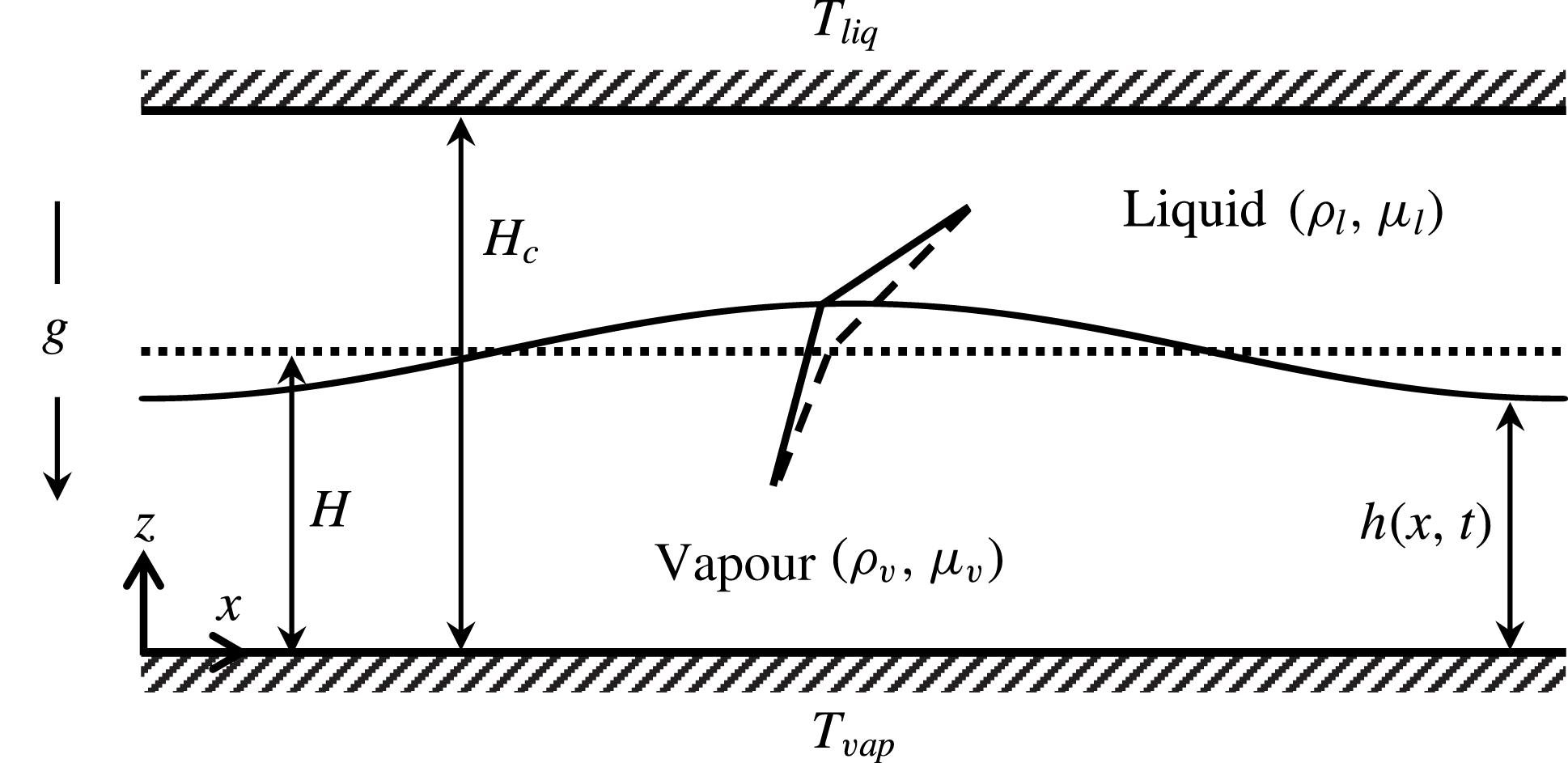
A flat interface between a liquid and its vapour may be rendered unstable by evaporation (Berg, Boudart & Acrivos Reference Berg, Boudart and Acrivos1966; Miller Reference Miller1973; Burelbach, Bankoff & Davis Reference Burelbach, Bankoff and Davis1988). This instability deforms the interface and sets up flow within each phase. In order to understand the physics of evaporative instability, let us consider a liquid–vapour bilayer confined between two flat plates as shown in figure 1. The flat plate in contact with the liquid is heated and maintained at temperature,
 $T_{liq}$
, while the flat plate contacting the vapour phase is maintained at a colder temperature,
 $T_{vap}$
. In order to focus solely on the mechanism of interfacial instability arising due to evaporation, let us momentarily ignore gravity and also assume that there is no sub-cooled condensation. Then, in the base state, the interface is flat and stationary with no flow in both phases as the entire set-up is hermetically sealed (cf. the dotted line in figure 1). The temperature profile is characterized purely by thermal conduction. The dashed lines in figure 1 depict the local temperature profile at the interface. The conductive heat fluxes between the two phases at the interface are balanced resulting in no evaporative mass flux. When a mechanical perturbation is imposed on the base interface profile, the crest is closer to the hot plate and the trough is closer to the cold plate (cf. the solid curve in figure 1). This results in a stronger thermal gradient in the liquid phase and weaker thermal gradient in the vapour phase at the crest, as evident from the slope of perturbed temperature profiles in figure 1 (solid lines). This implies that more heat is transferred from the liquid to the interface while less heat is taken away by the vapour from the interface. This imbalance in conductive heat fluxes causes evaporation at the crest and the crest moves further upward, reinforcing the perturbation and making the interface unstable. Now evaporation is accompanied by fluid flow in both phases and the wavelength of instability is therefore selected by the interfacial tension and viscous effects. Based on this line of reasoning, it can then be seen that heating from the vapour side stabilizes the interface. Evaporative instability is thus similar in nature to other phase-change instabilities such as solidification and electrodeposition where a temperature gradient or an electrochemical potential gradient normal to the interface drives the instability (Johns & Narayanan Reference Johns and Narayanan2002).
Physics of evaporation-driven instability when heated from liquid side (
 $T_{liq}>T_{vap}$
). The dotted horizontal line denotes the flat interface in the base state (
 $z=H$
), while the dashed lines denote the local base temperature profiles at the interface. The solid curve denotes the perturbed interface (
 $z=h(x,t)$
), while the solid lines denote the local temperature profiles after perturbation.
Owing to applications in several technological processes such as heat exchangers, film coatings and fabrication of patterned substrates, a detailed investigation of the dynamics of a liquid–vapour interface undergoing evaporation is of significance (Lin Reference Lin2012; Chatterjee, Plawsky & Wayner Reference Chatterjee, Plawsky and Wayner2013). Also, it is often found in pool boiling experiments that a layer of the less dense vapour phase is stably sustained below the heavier liquid phase (Rajabi & Winterton Reference Rajabi and Winterton1987). The formation of such a stable vapour film near the heated surface is called the boiling crisis phenomenon and results in unfavourable burnout of heat exchangers (Theofanous et al. Reference Theofanous, Tu, Dinh and Dinh2002). Thus, the heavy-over-light fluid configuration susceptible to the classic Rayleigh–Taylor (R–T) instability may be stabilized by evaporative phase change (Adham-Khodaparast, Kawaji & Antar Reference Adham-Khodaparast, Kawaji and Antar1995).
The current work focuses on the interfacial dynamics of an evaporating bilayer system, first in the absence of gravity and then in the presence of gravity where a heavy-over-light configuration is of interest. The former case helps to gain a comprehensive understanding of the physics of the evaporative instability. In addition, the results of this analysis also find applications in the constrained vapour bubble (CVB) experiments carried out in microgravity conditions (Chatterjee et al. Reference Chatterjee, Plawsky and Wayner2013) and flow boiling condensation experiments (Kharangate, ONeill & Mudawar Reference Kharangate, Oneill and Mudawar2016), when conducted in pool boiling mode. The second case of destabilizing gravity is motivated by its applications to boiling crisis phenomenon. We briefly discuss the earlier works relevant to the current work.
Miller (Reference Miller1973) and Palmer (Reference Palmer1976) were amongst the early investigators to study the linear instability associated with evaporative phase change. They considered a liquid–vapour interface propagating at a constant speed due to finite non-zero evaporative mass flux in the base state. They showed that vapour recoil is the dominant cause of instability under such conditions. Margerit et al. (Reference Margerit, Colinet, Lebon, Iorio and Legros2003) studied this case under non-equilibrium conditions at the interface and showed that interfacial non-equilibrium enhances the phase-change instability. In addition, they showed that phase change suppresses the thermocapillary Marangoni instability. Stability of a stationary interface between quiescent fluids with no evaporative mass flux in the base state have also been carried out by a number of authors. Ozen & Narayanan (Reference Ozen and Narayanan2004) showed that a static liquid–vapour interface becomes unstable when heated from the liquid side. They also showed that the vapour phase significantly stabilizes the system thereby emphasizing the importance of an active vapour phase. McFadden et al. (Reference McFadden, Coriell, Gurski and Cotrell2007) considered a bilayer system near its thermodynamic critical state and showed that entropy difference between the phases has significant effect on the instability. For significant difference in entropy between the phases (like a water–water vapour system), they showed that the system can become unstable only when heated from the liquid side. They also attributed the insignificance of Marangoni instability during phase change to this significant difference in entropy between the phases. By artificially lowering the entropy difference, they showed that the Marangoni effect may become important. For bilayer systems far away from the thermodynamic critical state, McFadden & Coriell (Reference McFadden and Coriell2009) reported the emergence of an oscillatory instability when heated from the vapour side. Weak nonlinear results of Guo & Narayanan (Reference Guo and Narayanan2010) showed that depending upon the aspect ratio of the geometry, evaporative instability may show either supercritical or subcritical behaviour.
The linear stability analyses carried out by Hsieh were the earliest to suggest that R–T instability can be stabilized by evaporation (Hsieh Reference Hsieh1972, Reference Hsieh1978). He studied the case of inviscid fluids and showed that the linear growth rates associated with the classic R–T instability decrease in the presence of phase change. His results showed that the cutoff wavenumber however was not affected by phase change. Ho (Reference Ho1980) extended his analysis to viscous fluids and showed that a coupling between the viscous effects and phase change was instrumental in shifting the cutoff wavenumber to longer waves, decreasing the range of unstable wavenumbers. Adham-Khodaparast et al. (Reference Adham-Khodaparast, Kawaji and Antar1995) re-derived the results of Ho (Reference Ho1980) and obtained the dispersion relation in a convenient form that reduces to the classic R–T case in the absence of phase change as well as to the case of Hsieh (Reference Hsieh1978) in the inviscid limit. These works used a phenomenological constant to decouple the temperature and velocity fields. However, Ozen & Narayanan (Reference Ozen and Narayanan2006) showed that the phenomenological constant is, in fact, strongly dependent on the perturbation wavenumber and has to be determined as an output of the problem rather than an input parameter. Recent works of Kanatani (Reference Kanatani2010), Kim & Kim (Reference Kim and Kim2016), Konovalov, Lyubimov & Lyubimova (Reference Konovalov, Lyubimov and Lyubimova2016) and Konovalov, Lyubimov & Lyubimova (Reference Konovalov, Lyubimov and Lyubimova2017) based on linear theory have also shown the possibility of suppression of R–T instability by phase change.
The nonlinear dynamics of an evaporating interface can be well captured using thin-film models as demonstrated by Burelbach et al. (Reference Burelbach, Bankoff and Davis1988) and Oron, Davis & Bankoff (Reference Oron, Davis and Bankoff1997) among others. These works use one-sided models, ignore vapour dynamics and correspond to a liquid evaporating into a passive medium. Total mass of the evaporating liquid is therefore not conserved with time, which limits the relevance of their models to thin films that disappear due to evaporation into an open ambient medium. Nonlinear one-sided models used by Bestehorn & Merkt (Reference Bestehorn and Merkt2006) and Narendranath et al. (Reference Narendranath, Hermanson, Kolkka, Struthers and Allen2014) showed evaporative stabilization of R–T instability. Narendranath et al. (Reference Narendranath, Hermanson, Kolkka, Struthers and Allen2014) accounted for additional effects of vapour recoil in their model. To the best of our knowledge, only Kanatani & Oron (Reference Kanatani and Oron2011) have used a two-sided nonlinear model to investigate the interface dynamics in the presence of evaporation. Under reasonable assumptions of small density and viscosity ratios, they obtained a simplified model that incorporated the majority of the relevant physics. In addition, their study is limited to creeping flow conditions. In this study, we retain both momentum and thermal inertia to investigate their role in the interfacial dynamics and show that they can play a significant role. In addition, as our model is not restricted to small density and viscosity ratios, its validity extends to systems that may have similar viscosities and densities such as systems near thermodynamic critical point (cf. McFadden et al. Reference McFadden, Coriell, Gurski and Cotrell2007). Our model also differs from Kanatani & Oron (Reference Kanatani and Oron2011) in the treatment of interfacial conditions. While, their model incorporates a non-equilibrium description of the interface based on the Hertz–Knudsen theory, our model assumes local thermodynamic equilibrium based on the Clausius–Clapeyron equation. It will be shown that this equilibrium assumption is capable of capturing all the relevant dynamics of the interface. Further, we have also included the effect of disjoining pressure to investigate the rupture dynamics of the interface.
As described earlier, evaporation of a quiescent interface is governed by an imbalance in the conductive heat fluxes at the interface. The characteristic velocity scale associated with the instability is therefore obtained by a balance of conduction and latent heat terms in the interfacial energy balance. In this work, we have chosen the water–water vapour bilayer as a representative system to study the dynamics of an evaporating interface. We show that the typical Reynolds number associated with the instability is of
 $O(1)$
, even for thin bilayer systems of 0.7 mm depth. Momentum inertia is therefore expected not to be insignificant. In addition, the properties of water and vapour at saturation conditions of
 $100\,^{\circ }\text{C}$
and 1 atm. as listed in table 1 suggest that the Prandtl numbers of both fluids are close to 1. Hence, thermal inertia also contributes to the dynamics of an evaporating interface. In this work, we consider a nonlinear model for a two-sided evaporating bilayer that include the effects of inertia and gravity. The objective is to investigate the dynamics towards either nonlinear saturated states or to film rupture.
Thermophysical properties of water and water vapour used for calculations. A value of
 $H_{c}=0.7~\text{mm}$
is used in calculating the dimensionless groups.

The nonlinear model in this study assumes that both phases are thin layers. The method of weighted-residual integral boundary layer (WRIBL) for a confined two-phase system is used. The WRIBL method was first introduced by Ruyer-Quil & Manneville (Reference Ruyer-Quil and Manneville2000) in the context of modelling of a thin liquid film falling down an inclined plane. They showed that the model so developed was successful in accurately predicting the stability threshold. In addition, it was also able to overcome the finite-time singularities observed far from threshold in earlier modelling attempts such as Benney’s equation, the Shkadov model or their own earlier model based on the mixed integral-collocation method. Further, they also conclusively showed that the Galerkin method was the most efficient weighted-residual strategy in obtaining evolution equations, as compared to any other technique (Ruyer-Quil & Manneville Reference Ruyer-Quil and Manneville2002). The WRIBL method has since then been used to include heat transfer in falling liquid films and a good review of these works can be found in Kalliadasis et al. (Reference Kalliadasis, Ruyer-Quil, Scheid and Velarde2011). The method has also been successfully applied to model two-phase flows in narrow planar channels (Dietze & Ruyer-Quil Reference Dietze and Ruyer-Quil2013) as well as circular tubes (Dietze & Ruyer-Quil Reference Dietze and Ruyer-Quil2015). In this work, we follow the two-phase modelling as outlined in Dietze & Ruyer-Quil (Reference Dietze and Ruyer-Quil2013) and extend it to include heat transfer in both phases. Our treatment of heat transfer is, in effect, an extension of the ‘improved KKD (Kalliadasis–Kiyashko–Demekhin)’ model for non-isothermal falling films (Trevelyan & Kalliadasis Reference Trevelyan and Kalliadasis2004) to a two-phase confined system. In contrast to the one-sided evaporation models in the literature, our model is relevant to a liquid evaporating into vapour within a closed confinement.
The paper is structured as follows. A detailed derivation of the reduced-order model is discussed in § 2, along with the numerical methodology employed to solve the governing equations. In § 3, significant results obtained from the model are discussed. Both zero-gravity evaporation as well as evaporation in the presence of destabilizing gravity are explored. We conclude by summarizing the key results of our work in § 4.
2 Mathematical model
Consider a bilayer system of a liquid lying above its own vapour confined between two flat plates as depicted in figure 1. The distance between the flat plates is denoted by
 $H_{c}$
and the undisturbed interface is located at
 $z=H$
. Both fluids are considered to be Newtonian with constant thermophysical properties. All liquid and vapour variables are denoted with subscripts
 $l$
and
 $v$
. The densities, viscosities, thermal conductivities and thermal diffusivities of the two phases are denoted by
 $\unicode[STIX]{x1D70C}_{i}$
,
 $\unicode[STIX]{x1D707}_{i}$
,
 ${\mathcal{K}}_{i}$
and
 $\unicode[STIX]{x1D6FC}_{i}\;(i=l,v)$
. The horizontal and vertical components of velocity are denoted by
 $u_{i}$
and
 $w_{i}$
. The bottom wall in contact with the vapour phase is maintained at temperature
 $T_{vap}$
and the top wall in contact with the liquid phase is maintained at temperature
 $T_{liq}$
. Gravity acts downward. Both phases are assumed to be thin films and therefore the long-wave approximation,
 $(H_{c}\ll \unicode[STIX]{x1D6EC})$
, is used where
 $\unicode[STIX]{x1D6EC}$
is the characteristic horizontal length scale arising from the instability. This separation of length scales helps us to obtain a reduced set of evolution equations for the interface position,
 $h$
, the phase flow rates,
 $q_{l}$
and
 $q_{v}$
, as well as the interface temperature,
 $\unicode[STIX]{x1D703}$
. In thin films, buoyancy convection is deemed to be insignificant (cf. Zhang Reference Zhang and Savino2006) and is therefore ignored in this study. We now proceed to derive the long-wave equations.
2.1 Long-wave equations
We first introduce the following scales to non-dimensionalize the variables, denoted with an asterisk.
 $$\begin{eqnarray}x=\frac{x^{\ast }}{\unicode[STIX]{x1D6EC}},\quad z=\frac{z^{\ast }}{H_{c}},\quad t=\frac{t^{\ast }}{\unicode[STIX]{x1D6EC}/U},\quad u_{i}=\frac{u_{i}^{\ast }}{U},\quad w_{i}=\frac{w_{i}^{\ast }}{\unicode[STIX]{x1D716}U},\quad p_{i}=\frac{p_{i}^{\ast }}{\unicode[STIX]{x1D707}_{i}U/H_{c}},\quad T_{i}=\frac{T_{i}^{\ast }-T_{liq}}{\unicode[STIX]{x0394}T}.\end{eqnarray}$$
Here,
 $\unicode[STIX]{x1D716}$
is a small parameter defined as
 $\unicode[STIX]{x1D716}=H/\unicode[STIX]{x1D6EC}$
and
 $\unicode[STIX]{x0394}T=T_{vap}-T_{liq}$
represents the imposed temperature difference across the plates. The characteristic velocity scale,
 $U=({\mathcal{K}}_{l}|\unicode[STIX]{x0394}T|)/(\unicode[STIX]{x1D70C}_{v}{\mathcal{L}}H_{c})$
, is obtained by a balance of conduction and latent heat terms in the interfacial energy balance. As expected, the characteristic velocity ought to be proportional to the magnitude of
 $\unicode[STIX]{x0394}T$
, which would be the true control variable in a physical experiment.
We then obtain the non-dimensional equations using the above scales. These equations, neglecting the terms of
 $O(\unicode[STIX]{x1D716}^{2})$
and smaller, are
 $$\begin{eqnarray}\frac{\unicode[STIX]{x2202}u_{i}}{\unicode[STIX]{x2202}x}+\frac{\unicode[STIX]{x2202}w_{i}}{\unicode[STIX]{x2202}z}=0,\quad i=l,v\end{eqnarray}$$
 $$\begin{eqnarray}-\unicode[STIX]{x1D716}\frac{\unicode[STIX]{x2202}p_{l}}{\unicode[STIX]{x2202}z}-\unicode[STIX]{x1D716}G=0,\quad -\unicode[STIX]{x1D716}\frac{\unicode[STIX]{x2202}p_{v}}{\unicode[STIX]{x2202}z}-\unicode[STIX]{x1D716}\frac{\unicode[STIX]{x1D70C}}{\unicode[STIX]{x1D707}}G=0\end{eqnarray}$$
 $$\begin{eqnarray}\displaystyle & \displaystyle \unicode[STIX]{x1D716}Re\left(\frac{\unicode[STIX]{x2202}u_{l}}{\unicode[STIX]{x2202}t}+u_{l}\frac{\unicode[STIX]{x2202}u_{l}}{\unicode[STIX]{x2202}x}+w_{l}\frac{\unicode[STIX]{x2202}u_{l}}{\unicode[STIX]{x2202}z}\right)=-\unicode[STIX]{x1D716}\frac{\unicode[STIX]{x2202}p_{l}}{\unicode[STIX]{x2202}x}+\frac{\unicode[STIX]{x2202}^{2}u_{l}}{\unicode[STIX]{x2202}z^{2}} & \displaystyle\end{eqnarray}$$
 $$\begin{eqnarray}\displaystyle & \displaystyle \unicode[STIX]{x1D716}\frac{\unicode[STIX]{x1D70C}}{\unicode[STIX]{x1D707}}Re\left(\frac{\unicode[STIX]{x2202}u_{v}}{\unicode[STIX]{x2202}t}+u_{v}\frac{\unicode[STIX]{x2202}u_{v}}{\unicode[STIX]{x2202}x}+w_{v}\frac{\unicode[STIX]{x2202}u_{v}}{\unicode[STIX]{x2202}z}\right)=-\unicode[STIX]{x1D716}\frac{\unicode[STIX]{x2202}p_{v}}{\unicode[STIX]{x2202}x}+\frac{\unicode[STIX]{x2202}^{2}u_{v}}{\unicode[STIX]{x2202}z^{2}} & \displaystyle\end{eqnarray}$$
 $$\begin{eqnarray}\unicode[STIX]{x1D716}Re\,Pr_{l}\left(\frac{\unicode[STIX]{x2202}T_{l}}{\unicode[STIX]{x2202}t}+u_{l}\frac{\unicode[STIX]{x2202}T_{l}}{\unicode[STIX]{x2202}x}+w_{l}\frac{\unicode[STIX]{x2202}T_{l}}{\unicode[STIX]{x2202}z}\right)=\frac{\unicode[STIX]{x2202}^{2}T_{l}}{\unicode[STIX]{x2202}z^{2}}\end{eqnarray}$$
and
 $$\begin{eqnarray}\unicode[STIX]{x1D716}\frac{{\mathcal{K}}\unicode[STIX]{x1D70C}}{\unicode[STIX]{x1D707}}Re\,Pr_{v}\left(\frac{\unicode[STIX]{x2202}T_{v}}{\unicode[STIX]{x2202}t}+u_{v}\frac{\unicode[STIX]{x2202}T_{v}}{\unicode[STIX]{x2202}x}+w_{v}\frac{\unicode[STIX]{x2202}T_{v}}{\unicode[STIX]{x2202}z}\right)={\mathcal{K}}\frac{\unicode[STIX]{x2202}^{2}T_{v}}{\unicode[STIX]{x2202}z^{2}},\end{eqnarray}$$
where several parameters appear in the above equations and are defined below
 $$\begin{eqnarray}\unicode[STIX]{x1D70C}=\frac{\unicode[STIX]{x1D70C}_{v}}{\unicode[STIX]{x1D70C}_{l}},\quad \unicode[STIX]{x1D707}=\frac{\unicode[STIX]{x1D707}_{v}}{\unicode[STIX]{x1D707}_{l}},\quad {\mathcal{K}}=\frac{{\mathcal{K}}_{v}}{{\mathcal{K}}_{l}},\quad Re=\frac{\unicode[STIX]{x1D70C}_{l}UH_{c}}{\unicode[STIX]{x1D707}_{l}}\quad G=\frac{\unicode[STIX]{x1D70C}_{l}gH_{c}^{2}}{\unicode[STIX]{x1D707}_{l}U},\quad Pr_{i}=\frac{\unicode[STIX]{x1D707}_{i}}{\unicode[STIX]{x1D70C}_{i}\unicode[STIX]{x1D6FC}_{i}},\quad i=l,v.\end{eqnarray}$$
Equations (2.2)–(2.5) are the long-wave equations consistent with the first-order approximation. To arrive at the above governing equations, we have assumed the Reynolds (
 $Re$
) and Prandtl numbers
 $(Pr_{i})$
to be of
 $O(1)$
. A quick calculation using properties of water from table 1, shows that the Reynolds number is indeed of
 $O(1)$
for moderate temperature differences, when
 $\unicode[STIX]{x0394}T\sim O(1)$
. Prandtl numbers of the fluids are also close to 1. Therefore, inertial effects are not ignored.
The inertial terms appear in the horizontal component of the momentum balance, equation (2.4), but do not contribute to the vertical component, equation (2.3), at this order. This allows us to integrate (2.3) in order to obtain the evolution equations. The effects of both momentum and thermal inertia have been retained. We also assume the viscosity ratio,
 $\unicode[STIX]{x1D707}$
, and density ratio,
 $\unicode[STIX]{x1D70C}$
, to be of
 $O(1)$
. In practice, both of these ratios for a typical liquid–vapour system are much smaller than
 $O(1)$
. Retaining these quantities only extends the validity of our model for systems that may have similar viscosities and densities such as systems near the thermodynamic critical point (cf. McFadden et al.
Reference McFadden, Coriell, Gurski and Cotrell2007). To obtain (2.5b
) in the given form, the energy balance in the vapour phase was multiplied throughout by
 ${\mathcal{K}}$
. This form of the energy balance makes it convenient to apply the WRIBL technique as we shall see later on. The governing equations are closed using appropriate boundary conditions. These conditions at the walls are:
 $$\begin{eqnarray}u_{v}=w_{v}=0,\quad T_{v}=1\quad \text{at }z=0\end{eqnarray}$$
and
 $$\begin{eqnarray}u_{l}=w_{l}=0,\quad T_{l}=0\quad \text{at }z=1.\end{eqnarray}$$
These correspond to the no-slip, no-penetration and constant temperature at both walls. At the interface, mass balance and kinematics give
 $$\begin{eqnarray}w_{l}-u_{l}\frac{\unicode[STIX]{x2202}h}{\unicode[STIX]{x2202}x}-\frac{\unicode[STIX]{x2202}h}{\unicode[STIX]{x2202}t}=\unicode[STIX]{x1D70C}\left(w_{v}-u_{v}\frac{\unicode[STIX]{x2202}h}{\unicode[STIX]{x2202}x}-\frac{\unicode[STIX]{x2202}h}{\unicode[STIX]{x2202}t}\right).\end{eqnarray}$$
The continuity of velocity at the interface gives
 $$\begin{eqnarray}u_{l}=u_{v}\quad \text{and}\quad w_{l}=w_{v}.\end{eqnarray}$$
The tangential and normal stress balances at the interface are
 $$\begin{eqnarray}\unicode[STIX]{x1D707}\frac{\unicode[STIX]{x2202}u_{v}}{\unicode[STIX]{x2202}z}=\frac{\unicode[STIX]{x2202}u_{l}}{\unicode[STIX]{x2202}z}\quad \text{and}\quad \unicode[STIX]{x1D707}p_{v}-p_{l}=-\unicode[STIX]{x1D716}^{2}\frac{1}{Ca}\frac{\unicode[STIX]{x2202}^{2}h}{\unicode[STIX]{x2202}x^{2}}-P_{D},\quad \text{where }Ca=\frac{\unicode[STIX]{x1D707}_{l}U}{\unicode[STIX]{x1D6FE}}.\end{eqnarray}$$
Thermocapillarity is unimportant in the presence of phase change (Margerit et al.
Reference Margerit, Colinet, Lebon, Iorio and Legros2003; Ozen & Narayanan Reference Ozen and Narayanan2004; Kanatani & Oron Reference Kanatani and Oron2011) and therefore has been neglected in the tangential stress balance. In order to retain the effects of surface tension in the normal stress balance, the capillary number,
 $Ca$
, is assumed to be
 $O(\unicode[STIX]{x1D716}^{2})$
or smaller. The effects of vapour recoil, which only appear at
 $O(\unicode[STIX]{x1D716}^{2})$
have been neglected in the normal stress balance.
 $P_{D}$
in the above equation accounts for the disjoining pressure arising due to intermolecular forces. The effect of disjoining pressure becomes relevant only when a film thins to such small length scales (approximately 100 nm) that the long-range intermolecular forces such as van der Waals and London forces become important (Israelachvili Reference Israelachvili2011). We, therefore, study the influence of this term only in our discussion on rupture dynamics and ignore this term in the rest of the results. As our working fluid, water is a polar molecule, our disjoining pressure consists of the usual Hamaker term due to van der Waals forces as well as an additional term that takes into account the effect of electric bilayer formation in polar fluids (Oron et al.
Reference Oron, Davis and Bankoff1997; Ajaev Reference Ajaev2005) as given below
 $$\begin{eqnarray}P_{D}=A_{\unicode[STIX]{x1D6F7}}\left(\frac{1}{h^{3}}-\frac{1}{(1-h)^{3}}\right)-A_{pol}(\exp ^{-\unicode[STIX]{x1D6FD}h}+\exp ^{-\unicode[STIX]{x1D6FD}(1-h)}),\end{eqnarray}$$
where
 $A_{\unicode[STIX]{x1D6F7}}=A_{h}/6\unicode[STIX]{x03C0}\unicode[STIX]{x1D6FE}H_{c}^{2}$
is the non-dimensional Hamaker constant and
 $A_{pol}=K_{s}H_{c}/\unicode[STIX]{x1D6FE}$
represents the strength of polar interaction (Ajaev Reference Ajaev2005). The Hamaker constant (
 $A_{h}$
) is taken to be
 $10^{-19}J$
(Israelachvili Reference Israelachvili2011).
The energy balance at the interface is given by
 $$\begin{eqnarray}j\equiv \unicode[STIX]{x1D716}\left(w_{v}-u_{v}\frac{\unicode[STIX]{x2202}h}{\unicode[STIX]{x2202}x}-\frac{\unicode[STIX]{x2202}h}{\unicode[STIX]{x2202}t}\right)=E\left({\mathcal{K}}\frac{\unicode[STIX]{x2202}T_{v}}{\unicode[STIX]{x2202}z}-\frac{\unicode[STIX]{x2202}T_{l}}{\unicode[STIX]{x2202}z}\right),\end{eqnarray}$$
where
 $j$
represents the evaporative mass flux and
 $E$
is the evaporation number given as
 $E=({\mathcal{K}}_{l}\unicode[STIX]{x0394}T)/(\unicode[STIX]{x1D70C}_{v}U{\mathcal{L}}H_{c})$
and is assumed to be of
 $O(1)$
. This is indeed true because
 $E=1$
when heated from the vapour side and
 $E=-1$
when heated from the liquid side.
We assume thermodynamic equilibrium and continuity of temperature along the interface. This assumption is borne out of the past work of Huang & Joseph (Reference Huang and Joseph1992), who concluded that this was valid for low evaporation rates. This is consistent with our model where the base state evaporation rate is zero and where evaporation takes place only upon perturbation. It might be noted that non-equilibrium relationships would be appropriate for problems with large evaporation rates (cf. for example Shankar & Deshpande Reference Shankar and Deshpande1990; Ward & Stanga Reference Ward and Stanga2001; Kanatani Reference Kanatani2010; Persad & Ward Reference Persad and Ward2016). To this end, we use the Clausius–Clapeyron equation as the equilibrium condition at the interface and give it in its linear approximation as
 $$\begin{eqnarray}\unicode[STIX]{x1D716}\unicode[STIX]{x1D707}(p_{v}-p_{ref})=\unicode[STIX]{x1D6F7}(T_{v}-T_{ref})\quad \text{where }\unicode[STIX]{x1D6F7}=\frac{S\unicode[STIX]{x0394}TH_{c}}{\unicode[STIX]{x1D707}_{l}U},\end{eqnarray}$$
where
 $S$
is a dimensional coefficient that appears in the linearized Clausius–Clapeyron equation and where
 $p_{ref}$
is the saturation pressure at a reference temperature,
 $T_{ref}$
. The details of determining
 $S$
are given in appendix A. In addition, the continuity of temperature at the interface is given by
 $$\begin{eqnarray}T_{l}=T_{v}.\end{eqnarray}$$
Equations (2.2)–(2.14) constitute the complete set of long-wave equations that govern the system.
We now proceed to derive the evolution equations for the interface location from the above long-wave equations. These are obtained by integrating the vertical component of the momentum balance (2.3) from a point
 $z$
inside the domain of each phase to the interface,
 $h(x,t)$
. Eliminating the pressure fields from the integrated equations using the transverse component of the momentum balance, the normal stress condition and the Clausius–Clapeyron equation we get
 $$\begin{eqnarray}\unicode[STIX]{x1D716}Re\left(\frac{\unicode[STIX]{x2202}u_{l}}{\unicode[STIX]{x2202}t}+u_{l}\frac{\unicode[STIX]{x2202}u_{l}}{\unicode[STIX]{x2202}x}+w_{l}\frac{\unicode[STIX]{x2202}u_{l}}{\unicode[STIX]{x2202}z}\right)=-\unicode[STIX]{x1D716}\unicode[STIX]{x1D6F7}\frac{\unicode[STIX]{x2202}\unicode[STIX]{x1D703}}{\unicode[STIX]{x2202}x}-\unicode[STIX]{x1D716}^{3}\frac{1}{Ca}\frac{\unicode[STIX]{x2202}^{3}h}{\unicode[STIX]{x2202}x^{3}}-\unicode[STIX]{x1D716}\frac{\unicode[STIX]{x2202}P_{D}}{\unicode[STIX]{x2202}x}-\unicode[STIX]{x1D716}G\frac{\unicode[STIX]{x2202}h}{\unicode[STIX]{x2202}x}+\frac{\unicode[STIX]{x2202}^{2}u_{l}}{\unicode[STIX]{x2202}z^{2}}\end{eqnarray}$$
and
 $$\begin{eqnarray}\unicode[STIX]{x1D716}\unicode[STIX]{x1D70C}Re\left(\frac{\unicode[STIX]{x2202}u_{v}}{\unicode[STIX]{x2202}t}+u_{v}\frac{\unicode[STIX]{x2202}u_{v}}{\unicode[STIX]{x2202}x}+w_{v}\frac{\unicode[STIX]{x2202}u_{v}}{\unicode[STIX]{x2202}z}\right)=-\unicode[STIX]{x1D716}\unicode[STIX]{x1D6F7}\frac{\unicode[STIX]{x2202}\unicode[STIX]{x1D703}}{\unicode[STIX]{x2202}x}-\unicode[STIX]{x1D716}\unicode[STIX]{x1D70C}G\frac{\unicode[STIX]{x2202}h}{\unicode[STIX]{x2202}x}+\unicode[STIX]{x1D707}\frac{\unicode[STIX]{x2202}^{2}u_{v}}{\unicode[STIX]{x2202}z^{2}}.\end{eqnarray}$$
Here,
 $\unicode[STIX]{x1D703}$
is the interface temperature given by
 $\unicode[STIX]{x1D703}=T_{l}|_{h}=T_{v}|_{h}$
. The above equations, viz., equation (2.15) along with (2.5), constitute the set of ‘boundary layer’ equations for this system. We now apply the WRIBL technique to derive a set of reduced-order evolution equations that govern the interface position,
 $h(x,t)$
, flow rates (
 $q_{l}(x,t),q_{v}(x,t)$
) and the interface temperature,
 $\unicode[STIX]{x1D703}(x,t)$
.
2.2 Weighted-residual integral method
To obtain the evolution equations for thin films with two active phases, we follow the weighted-residual integral boundary layer (WRIBL) methodology described by Dietze & Ruyer-Quil (Reference Dietze and Ruyer-Quil2013). They obtain evolution equations for a confined thin liquid film interacting with its surrounding gas. We extend their methodology for confined two-phase systems to include inertial effects associated with heat transfer as well. Our treatment of heat transfer equation is similar to the one-sided ‘KKD’ (Kalliadasis et al. Reference Kalliadasis, Demekhin, Ruyer-Quil and Velarde2003a ; Kalliadasis, Kiyashko & Demekhin Reference Kalliadasis, Kiyashko and Demekhin2003b ) and ‘improved KKD’ (Trevelyan & Kalliadasis Reference Trevelyan and Kalliadasis2004) models developed for non-isothermal falling thin films. We now proceed to describe the methodology.
First, we integrate the continuity equation (2.2) across the thickness of each phase. Then making use of the Leibnitz’s integration rule along with the no-penetration (2.7a,b ) and kinematic (2.8) conditions, we obtain
 $$\begin{eqnarray}(\unicode[STIX]{x1D70C}-1)\frac{\unicode[STIX]{x2202}h}{\unicode[STIX]{x2202}t}=-\!\left(\unicode[STIX]{x1D70C}\frac{\unicode[STIX]{x2202}q_{v}}{\unicode[STIX]{x2202}x}+\frac{\unicode[STIX]{x2202}q_{l}}{\unicode[STIX]{x2202}x}\right).\end{eqnarray}$$
In the above,
 $q_{v}$
and
 $q_{l}$
are flow rates associated with the respective phases and are defined as
 $$\begin{eqnarray}q_{v}=\int _{0}^{h}u_{v}\,\text{d}z,\quad q_{l}=\int _{h}^{1}u_{l}\,\text{d}z.\end{eqnarray}$$
Next, the boundary layer equations for both phases given by (2.5) and (2.15) are multiplied by appropriate weight functions and integrated across each film thickness. The resulting integral equations are then summed to give
 $$\begin{eqnarray}\int _{0}^{h}\mathit{BLE}_{v}F_{v}\,\text{d}z+\int _{h}^{1}\mathit{BLE}_{l}F_{l}\,\text{d}z=0,\end{eqnarray}$$
where
 $\mathit{BLE}_{i}$
are the boundary layer equations for the two phases given by (2.5) and (2.15) and
 $F_{i}$
are the appropriate weight functions, which shall be defined later. This procedure yields the evolution equations that govern the system. It should be noted that (2.18) represents a general weighted-residual methodology. Various weighted-residual strategies such as Galerkin, collocation, the method of moments and subdomains differ from each other only in their treatment of the unknowns being solved (such as
 $u,w,T$
) and the choice of the weight functions being employed (
 $F_{l},F_{v}$
). The Galerkin method offers the fastest convergence with minimum algebra (Ruyer-Quil & Manneville Reference Ruyer-Quil and Manneville2002) and is therefore adopted in this work.
Toward this, we decompose the horizontal velocity component and temperature as follows:
 $$\begin{eqnarray}u_{i}(x,z,t)=\underbrace{\hat{u} _{i}(x,z,t)}_{O(1)}+\underbrace{\tilde{u} _{i}(x,z,t)}_{O(\unicode[STIX]{x1D716})},\quad w_{v}=-\!\int _{0}^{z}\frac{\unicode[STIX]{x2202}u_{v}}{\unicode[STIX]{x2202}x}\,\text{d}z,\quad w_{l}=-\!\int _{1}^{z}\frac{\unicode[STIX]{x2202}u_{l}}{\unicode[STIX]{x2202}x}\,\text{d}z\end{eqnarray}$$
 $$\begin{eqnarray}T_{i}(x,z,t)=\underbrace{\hat{T}_{i}(x,z,t)}_{O(1)}+\underbrace{\tilde{T}_{i}(x,z,t)}_{O(\unicode[STIX]{x1D716})}.\end{eqnarray}$$
In the above, the hatted variables are of
 $O(1)$
and the variables with tilde denote their respective
 $O(\unicode[STIX]{x1D716})$
corrections. The vertical components of velocity (
 $w_{i}$
), as shown in (2.19a–c
), are obtained from horizontal velocity components by integrating the continuity equation. Next, the
 $O(1)$
contribution to the horizontal velocity components are chosen to satisfy the following conditions:
 $$\begin{eqnarray}\frac{\unicode[STIX]{x2202}^{2}\hat{u} _{l}}{\unicode[STIX]{x2202}z^{2}}=K_{l},\quad \frac{\unicode[STIX]{x2202}^{2}\hat{u} _{v}}{\unicode[STIX]{x2202}z^{2}}=K_{v},\quad \int _{0}^{h}\hat{u} _{v}\,\text{d}z=q_{v},\quad \int _{h}^{1}\hat{u} _{l}\,\text{d}z=q_{l}\end{eqnarray}$$
 $$\begin{eqnarray}\hat{u} _{v}|_{0}=0,\quad \hat{u} _{l}|_{1}=0,\quad \hat{u} _{v}|_{h}=\hat{u} _{l}|_{h},\quad \left.\unicode[STIX]{x1D707}\frac{\unicode[STIX]{x2202}\hat{u} _{v}}{\unicode[STIX]{x2202}z}\right|_{h}=\left.\frac{\unicode[STIX]{x2202}\hat{u} _{l}}{\unicode[STIX]{x2202}z}\right|_{h}.\end{eqnarray}$$
Equation (2.20) defines the leading-order velocity profile in each phase to be locally parabolic at each horizontal position. This assumption of parabolic velocity profile is justified for moderate Reynolds numbers and under these conditions, the
 $\unicode[STIX]{x1D716}$
-order corrections to the velocity profile remains small. From (2.20), it then follows that the velocity corrections are required to satisfy
 $$\begin{eqnarray}\int _{0}^{h}\tilde{u} _{v}\,\text{d}z=0,\quad \int _{h}^{1}\tilde{u} _{l}\,\text{d}z=0\end{eqnarray}$$
and
 $$\begin{eqnarray}\tilde{u} _{v}|_{0}=0,\quad \tilde{u} _{l}|_{1}=0,\quad \tilde{u} _{v}|_{h}=\tilde{u} _{l}|_{h},\quad \left.\unicode[STIX]{x1D707}\frac{\unicode[STIX]{x2202}\tilde{u} _{v}}{\unicode[STIX]{x2202}z}\right|_{h}=\left.\frac{\unicode[STIX]{x2202}\tilde{u} _{l}}{\unicode[STIX]{x2202}z}\right|_{h}.\end{eqnarray}$$
Now, as far as the energy equation is considered, the leading-order temperature profile is assumed to be locally linear. This assumption is justified because in our base state, there is no evaporation and the temperature fields in both phases exhibit a linear conduction profile. Therefore, it is reasonable to assume that at the onset of the long-wave instability, a locally linear temperature profile continues to persist. This assumption is, of course, not valid when evaporation rates are high and the temperature profiles exhibit significant deviations from linear profiles. Thus
 $\hat{T}_{l}$
and
 $\hat{T}_{v}$
satisfy
 $$\begin{eqnarray}\frac{\unicode[STIX]{x2202}^{2}\hat{T}_{l}}{\unicode[STIX]{x2202}z^{2}}=0,\quad \frac{\unicode[STIX]{x2202}^{2}\hat{T}_{v}}{\unicode[STIX]{x2202}z^{2}}=0\end{eqnarray}$$
and
 $$\begin{eqnarray}\hat{T}_{v}=\hat{T}_{l}=\unicode[STIX]{x1D703},\quad \hat{T}_{v}|_{0}=1,\quad \hat{T}_{l}|_{1}=0.\end{eqnarray}$$
It should be noted that the leading-order temperature profile does not satisfy the boundary condition (2.12). However, the weighted-residual strategy helps to satisfy this boundary condition, via the so-called tau method (Trevelyan & Kalliadasis Reference Trevelyan and Kalliadasis2004), while considering the integral associated with thermal diffusion term. The leading-order temperature profile as defined by (2.22) is valid for moderate Reynolds and Prandtl numbers. The
 $\unicode[STIX]{x1D716}$
-order corrections to the temperature profile remain small and from (2.22), they are required to satisfy
 $$\begin{eqnarray}\tilde{T}_{l}|_{h}=\tilde{T}_{v}|_{h}=0,\quad \tilde{T}_{v}|_{0}=0,\quad \tilde{T}_{l}|_{1}=0.\end{eqnarray}$$
Next, we substitute for velocity and temperature as given by (2.19) into (2.18). To obtain the evolution equations in terms of the variables
 $h,q_{l},q_{v}$
and
 $\unicode[STIX]{x1D703}$
alone, the unknown
 $O(\unicode[STIX]{x1D716})$
corrections to temperature and velocity profiles have to be eliminated. For this, in accordance with our first-order approximation, all terms of
 $O(\unicode[STIX]{x1D716}\tilde{u} )=O(\unicode[STIX]{x1D716}^{2})$
and smaller are neglected. We neglect altogether the velocity and temperature corrections appearing in the inertial terms (left-hand side of (2.5) and (2.15)) as these are of
 $O(\unicode[STIX]{x1D716}^{2})$
. This yields a simplified first-order model valid for moderate Reynolds and Prandtl numbers. The only terms that still contain the corrections of
 $O(\unicode[STIX]{x1D716})$
are due to the vertical component of momentum and thermal diffusion. These terms can be eliminated by a suitable choice of weight functions. The weight function associated with velocity shall be henceforth denoted by
 $F_{i}$
and that associated with temperature shall be denoted by
 $\hat{F}_{i}$
, where
 $i=l,v$
. The conditions imposed on
 $F_{i}$
to eliminate the
 $O(\unicode[STIX]{x1D716})$
corrections are given by
 $$\begin{eqnarray}\frac{\unicode[STIX]{x2202}^{2}F_{v}}{\unicode[STIX]{x2202}z^{2}}=A_{v},\quad \frac{\unicode[STIX]{x2202}^{2}F_{l}}{\unicode[STIX]{x2202}z^{2}}=A_{l},\quad F_{v}|_{0}=0,\quad F_{l}|_{1}=0,\quad F_{v}|_{h}=F_{l}|_{h},\quad \left.\unicode[STIX]{x1D707}\frac{\unicode[STIX]{x2202}F_{v}}{\unicode[STIX]{x2202}z}\right|_{h}=\left.\frac{\unicode[STIX]{x2202}F_{l}}{\unicode[STIX]{x2202}z}\right|_{h}.\end{eqnarray}$$
The two equations corresponding to the unknown variables
 $q_{v}$
and
 $q_{l}$
are obtained by choosing
 $(A_{v},A_{l})$
to be
 $(1,1)$
and
 $(1,-1)$
for the first and second equations respectively. The weight functions obtained from these choices of
 $(A_{v},A_{l})$
shall be denoted by
 $F_{i}^{(+)}$
and
 $F_{i}^{(-)}$
respectively. It is to be noted that these weight functions are completely determined using (2.24). The functional form of
 $\hat{F}_{l}$
and
 $\hat{F}_{v}$
is similar to the leading-order velocity profile (
 $\hat{u} _{l}$
and
 $\hat{u} _{v}$
). Similarly, the conditions imposed on
 $\hat{F}_{i}$
to eliminate the correction terms are given by
 $$\begin{eqnarray}\frac{\unicode[STIX]{x2202}^{2}\hat{F}_{v}}{\unicode[STIX]{x2202}z^{2}}=0,\quad \frac{\unicode[STIX]{x2202}^{2}\hat{F}_{l}}{\unicode[STIX]{x2202}z^{2}}=0,\quad \hat{F}_{v}|_{0}=0,\quad \hat{F}_{l}|_{1}=0,\quad \hat{F}_{v}|_{h}=\hat{F}_{l}|_{h},\quad \left.\frac{\unicode[STIX]{x2202}\hat{F}_{v}}{\unicode[STIX]{x2202}z}\right|_{h}=1.\end{eqnarray}$$
This then yields the dynamic equation for the interface temperature,
 $\unicode[STIX]{x1D703}$
. The final set of evolution equations are
 $$\begin{eqnarray}(\unicode[STIX]{x1D70C}-1)\frac{\unicode[STIX]{x2202}h}{\unicode[STIX]{x2202}t}=-\left(\unicode[STIX]{x1D70C}\frac{\unicode[STIX]{x2202}q_{v}}{\unicode[STIX]{x2202}x}+\frac{\unicode[STIX]{x2202}q_{l}}{\unicode[STIX]{x2202}x}\right)\end{eqnarray}$$
 $$\begin{eqnarray}\displaystyle & & \displaystyle \unicode[STIX]{x1D716}Re\left[L_{1}\frac{\unicode[STIX]{x2202}q_{l}}{\unicode[STIX]{x2202}t}+L_{2}\frac{\unicode[STIX]{x2202}q_{l}}{\unicode[STIX]{x2202}x}+M_{1}\frac{\unicode[STIX]{x2202}h}{\unicode[STIX]{x2202}x}+V_{1}\frac{\unicode[STIX]{x2202}q_{v}}{\unicode[STIX]{x2202}t}+V_{2}\frac{\unicode[STIX]{x2202}q_{v}}{\unicode[STIX]{x2202}x}\right]=-\unicode[STIX]{x1D716}\unicode[STIX]{x1D6F7}\frac{\unicode[STIX]{x2202}\unicode[STIX]{x1D703}}{\unicode[STIX]{x2202}x}(I_{v}^{(+)}+I_{l}^{(+)})\nonumber\\ \displaystyle & & \displaystyle \quad -\left(\unicode[STIX]{x1D716}^{3}\frac{1}{Ca}\frac{\unicode[STIX]{x2202}^{3}h}{\unicode[STIX]{x2202}x^{3}}+\unicode[STIX]{x1D716}\frac{\unicode[STIX]{x2202}P_{D}}{\unicode[STIX]{x2202}x}\right)I_{l}^{(+)}-\unicode[STIX]{x1D716}G\frac{\unicode[STIX]{x2202}h}{\unicode[STIX]{x2202}x}(\unicode[STIX]{x1D70C}I_{v}^{(+)}+I_{l}^{(+)})+\unicode[STIX]{x1D707}q_{v}+q_{l}\end{eqnarray}$$
 $$\begin{eqnarray}\displaystyle & & \displaystyle \unicode[STIX]{x1D716}Re\left[\bar{L}_{1}\frac{\unicode[STIX]{x2202}q_{l}}{\unicode[STIX]{x2202}t}+\bar{L}_{2}\frac{\unicode[STIX]{x2202}q_{l}}{\unicode[STIX]{x2202}x}+\bar{M}_{1}\frac{\unicode[STIX]{x2202}h}{\unicode[STIX]{x2202}x}+\bar{V}_{1}\frac{\unicode[STIX]{x2202}q_{v}}{\unicode[STIX]{x2202}t}+\bar{V}_{2}\frac{\unicode[STIX]{x2202}q_{v}}{\unicode[STIX]{x2202}x}\right]=-\unicode[STIX]{x1D716}\unicode[STIX]{x1D6F7}\frac{\unicode[STIX]{x2202}\unicode[STIX]{x1D703}}{\unicode[STIX]{x2202}x}(I_{v}^{(-)}+I_{l}^{(-)})\nonumber\\ \displaystyle & & \displaystyle \quad -\left(\unicode[STIX]{x1D716}^{3}\frac{1}{Ca}\frac{\unicode[STIX]{x2202}^{3}h}{\unicode[STIX]{x2202}x^{3}}+\unicode[STIX]{x1D716}\frac{\unicode[STIX]{x2202}P_{D}}{\unicode[STIX]{x2202}x}\right)I_{l}^{(-)}-\unicode[STIX]{x1D716}G\frac{\unicode[STIX]{x2202}h}{\unicode[STIX]{x2202}x}(\unicode[STIX]{x1D70C}I_{v}^{(-)}+I_{l}^{(-)})+\unicode[STIX]{x1D707}q_{v}-q_{l}\end{eqnarray}$$
and
 $$\begin{eqnarray}\displaystyle & & \displaystyle \unicode[STIX]{x1D716}Re\,Pr_{v}\left[\unicode[STIX]{x1D6F6}_{1}\frac{\unicode[STIX]{x2202}\unicode[STIX]{x1D703}}{\unicode[STIX]{x2202}t}+\unicode[STIX]{x1D6F6}_{2}\frac{\unicode[STIX]{x2202}\unicode[STIX]{x1D703}}{\unicode[STIX]{x2202}x}+\unicode[STIX]{x1D6F6}_{3}\frac{\unicode[STIX]{x2202}h}{\unicode[STIX]{x2202}x}+\unicode[STIX]{x1D6F6}_{4}\frac{\unicode[STIX]{x2202}q_{v}}{\unicode[STIX]{x2202}x}+\unicode[STIX]{x1D6F6}_{5}\frac{\unicode[STIX]{x2202}q_{l}}{\unicode[STIX]{x2202}x}\right]\nonumber\\ \displaystyle & & \displaystyle \quad =\frac{\unicode[STIX]{x1D716}h}{E}\left({\displaystyle \frac{\unicode[STIX]{x1D70C}{\displaystyle \frac{\unicode[STIX]{x2202}q_{v}}{\unicode[STIX]{x2202}x}}+{\displaystyle \frac{\unicode[STIX]{x2202}q_{l}}{\unicode[STIX]{x2202}x}}}{(\unicode[STIX]{x1D70C}-1)}}-\frac{\unicode[STIX]{x2202}q_{v}}{\unicode[STIX]{x2202}x}\right)-{\mathcal{K}}(\unicode[STIX]{x1D703}-1)-\frac{h\unicode[STIX]{x1D703}}{1-h}.\end{eqnarray}$$
Expressions for variables appearing in the above equations are given in the supplementary material available at https://doi.org/10.1017/jfm.2018.714. Equation (2.26) represents our nonlinear model consistent at first order. We now rescale the system by taking
 $\unicode[STIX]{x1D6EC}\rightarrow H_{c}$
, i.e.
 $\unicode[STIX]{x1D716}=1$
. This implies that in the discussion of our results, physical lengths in both horizontal and vertical directions are scaled with
 $H_{c}$
. As the characteristic length scale of instability (
 $\unicode[STIX]{x1D6EC}$
) is not known a priori, this rescaling eliminates the need to specify the unknown parameter
 $\unicode[STIX]{x1D716}$
as an input without any loss of generality in what follows.
2.3 Linear stability analysis
We carry out a linear stability analysis of the evolution equations (2.26) using the familiar method of modal analysis. The base state is assumed to be a static no-flow state with a linear temperature profile in each phase. The variables are perturbed around their base state as shown below:
 $$\begin{eqnarray}h=H+h^{\star }\text{e}^{\unicode[STIX]{x1D70E}t+\text{i}kx},\quad q_{i}=q_{i}^{\star }\text{e}^{\unicode[STIX]{x1D70E}t+\text{i}kx},\quad \unicode[STIX]{x1D703}=\frac{{\mathcal{K}}(1-H)}{H+{\mathcal{K}}(1-H)}+\unicode[STIX]{x1D703}^{\star }\text{e}^{\unicode[STIX]{x1D70E}t+\text{i}kx}.\end{eqnarray}$$
In the above, the starred variables denote the amplitudes of linear perturbations,
 $k$
is the spatial wavenumber and
 $\unicode[STIX]{x1D70E}$
is the corresponding linear growth rate. The results of linear stability of the WRIBL model (2.26) are compared with those of the long-wave starting equations (2.2)–(2.14). This will help us to check the linear results of the WRIBL model for moderate Reynolds and Prandtl numbers.
2.4 Nonlinear simulations
For nonlinear calculations, an initial wavy disturbance is imposed on the interface position and (2.26) are solved for one wavelength of the perturbation. The initial condition for the time-dependent variables are as given below
 $$\begin{eqnarray}h(x,0)=H+0.001\text{cos}(kx),\quad q_{i}(x,0)=0,\quad \unicode[STIX]{x1D703}(x,0)=\frac{{\mathcal{K}}(1-h(x,0))}{h(x,0)+{\mathcal{K}}(1-h(x,0))}.\end{eqnarray}$$
We use the Fourier spectral collocation technique to obtain numerical solutions. The spatial derivatives are approximated using the Fourier spectral discretization scheme as outlined in Labrosse (Reference Labrosse2011). A similar discretization scheme based on the Chebyshev polynomials has been detailed in Guo, Labrosse & Narayanan (Reference Guo, Labrosse and Narayanan2012). Fourier spectral collocation technique ensures that periodic conditions are imposed on the computational domain. This implies that each time-dependent variable and all its spatial derivatives are equal at both ends of the domain. Spectral methods offer exponential convergence with an increase in grid points because the error
 ${\approx}O[(1/N)^{N}]$
in such discretization schemes, where
 $N$
is the number of grid points. The time integration is performed using the NDSolve subroutine in Mathematica® v.10.3 which uses an adaptive procedure to determine the size of time stepping.
3 Results and discussion
The calculations are carried out using the physical properties of water and water vapour as listed in table 1. We sequentially investigate the system under various limits to gain a comprehensive understanding of the underlying physics of the problem. Both linear and nonlinear stability analyses are carried out for each of these limits and the observed results are discussed.
3.1 Evaporation in the absence of gravity
We commence the study where the system is subject to phase change alone. Gravity is not taken into account. This choice in assumptions physically corresponds to either extremely thin films or micro-gravity conditions, where the effect of gravity is negligible. In addition to its physical relevance, the results of this case are also vital in understanding the basic physics of evaporative instability. The possibility of condensation due to subcooling of vapour at the wall is ignored. Thus, phase change is expected to occur only at the liquid–vapour interface.
3.1.1 Inertialess creeping flow limit
In this sub-section, we discuss the results for the case where both momentum and thermal inertia are ignored. This corresponds to the creeping flow limit of vanishing Reynolds number (
 $Re\rightarrow 0$
). All past nonlinear studies of evaporating thin films have been restricted to this limit.
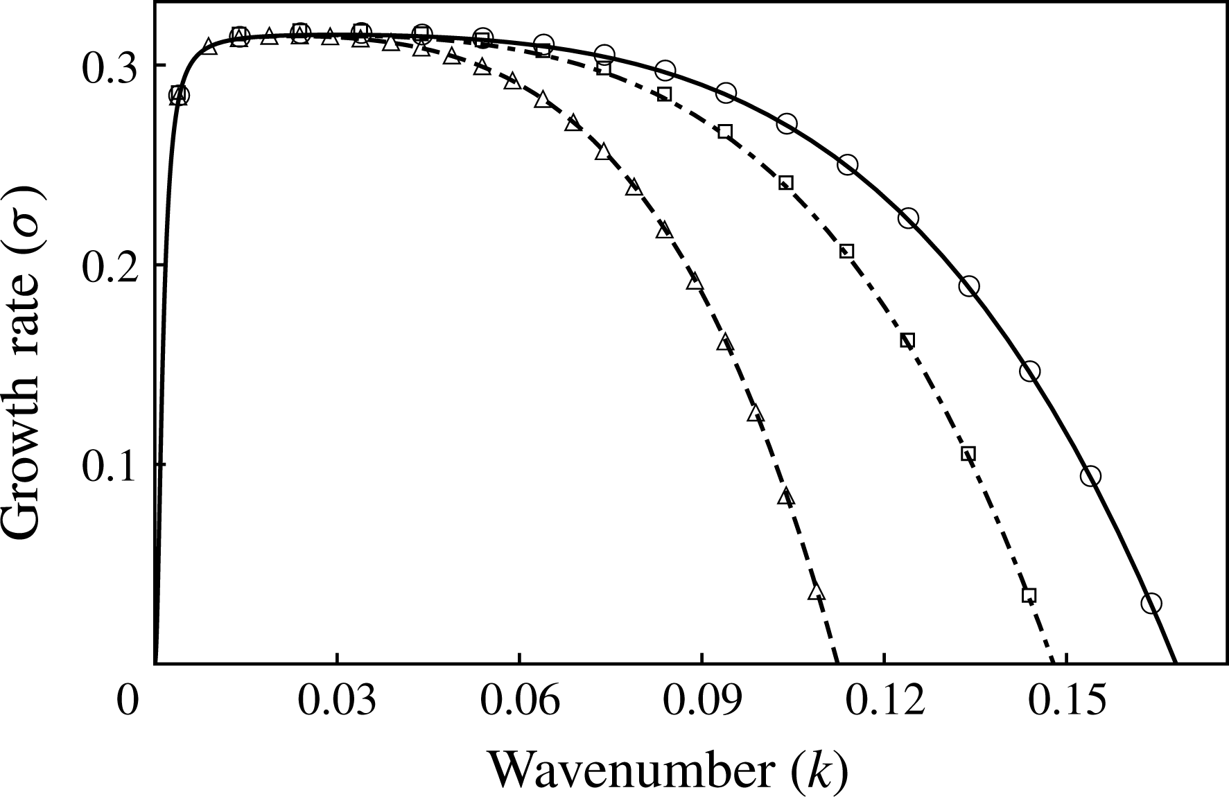
Growth rate versus wavenumber for evaporative instability when heated from liquid side (
 $E=-1$
) plotted for three different values of
 $\unicode[STIX]{x0394}T$
. The curves denote the growth rates obtained from (3.1) and the markers correspond to the growth rates obtained by linearizing the starting long-wave equations (2.2)–(2.14).
 $\unicode[STIX]{x0394}T=-1$
or
 $Ca=1.22\times 10^{-5}$
(dashed, triangles),
 $\unicode[STIX]{x0394}T=-3$
or
 $Ca=3.66\times 10^{-5}$
(dash-dotted, squares),
 $\unicode[STIX]{x0394}T=-5$
or
 $Ca=6.1\times 10^{-5}$
(solid, circles);
 $H=0.3$
.
Rescaled growth rate versus wavenumber using velocity scale,
 $U_{\unicode[STIX]{x1D6FE}}=\unicode[STIX]{x1D6FE}/\unicode[STIX]{x1D707}$
. The curves denote the growth rates obtained from (3.1) and the markers correspond to the growth rates obtained by linearizing the starting long-wave equations (2.2)–(2.14). (a) Evaporation when heated from the liquid side.
 $E=-1.22\times 10^{-5}$
(dashed, triangles),
 $E=-3.66\times 10^{-5}$
(dash-dotted, squares),
 $E=-6.1\times 10^{-5}$
(solid, circles); (b) evaporation when heated from the vapour side.
 $E=1.22\times 10^{-5}$
(dashed, triangles),
 $E=3.66\times 10^{-5}$
(dash-dotted, squares),
 $E=6.1\times 10^{-5}$
(solid, circles);
 $H=0.3$
.

The linear growth rate (
 $\unicode[STIX]{x1D70E}$
) obtained from linearization of the WRIBL model (2.26), in the creeping flow limit is given by:
 $$\begin{eqnarray}\unicode[STIX]{x1D70E}=\frac{\unicode[STIX]{x1D702}_{1}k^{2}+\unicode[STIX]{x1D702}_{2}k^{4}+\unicode[STIX]{x1D702}_{3}k^{6}}{\unicode[STIX]{x1D702}_{4}+\unicode[STIX]{x1D702}_{5}k^{2}}.\end{eqnarray}$$
The coefficients,
 $\unicode[STIX]{x1D702}_{i}$
, appearing in (3.1) are given in appendix B. In figure 2, we have plotted the growth rate (
 $\unicode[STIX]{x1D70E}$
) as a function of wavenumber when the system is heated from the liquid side (
 $\unicode[STIX]{x0394}T<0$
, i.e.
 $E=-1$
) for three practical cases of
 $\unicode[STIX]{x0394}T=-1\,^{\circ }\text{C}$
,
 $-3\,^{\circ }\text{C}$
and
 $-5\,^{\circ }\text{C}$
. Recalling that
 $U=({\mathcal{K}}_{l}|\unicode[STIX]{x0394}T|)/(\unicode[STIX]{x1D70C}_{v}{\mathcal{L}}H_{c})$
, these values of
 $\unicode[STIX]{x0394}T$
correspond to
 $Ca=1.22\times 10^{-5}$
,
 $3.66\times 10^{-5}$
and
 $6.1\times 10^{-5}$
. These values of
 $Ca$
validate the assumption made in § 2.1 that
 $Ca$
is of
 ${\sim}O(\unicode[STIX]{x1D716}^{2})$
or smaller. The curves in figure 2 correspond to growth rates obtained analytically from (3.1). The markers in figure 2 denote the numerically obtained growth rates by linearizing the starting long-wave equations (2.2)–(2.14) using the Chebyshev spectral collocation technique. It can be seen that they are identical, and for good reason. A departure from the two ways of calculating growth constants will only be seen when thermal and momentum inertia are taken into account, simply because closure of the long-wavelength model requires an assumed form for
 $\hat{u}$
and
 $\hat{T}$
. Even so, the agreement ought to be excellent for low inertia and small wavenumbers. Positive growth rates in figure 2 indicate that the system is unstable to long-wavelength disturbances when heated from the liquid side. The collapse of the dominant growth rates for all cases of
 $\unicode[STIX]{x0394}T$
to roughly the same value of
 $O(1)$
indicates that the chosen velocity scale is indeed correct. As noted earlier, the velocity scale contains the imposed temperature difference,
 $\unicode[STIX]{x0394}T$
. Therefore, in order to make fair comparisons on the basis of physics, it is helpful to use a velocity scale that does not change with the imposed
 $\unicode[STIX]{x0394}T$
. Hence, a velocity scale (
 $U_{\unicode[STIX]{x1D6FE}}=\unicode[STIX]{x1D6FE}/\unicode[STIX]{x1D707}_{l}$
) which depends only on fixed parameters of the system is used hereon to represent all our results in a physically meaningful way. With this choice of velocity scale,
 $Ca=1$
and
 $E$
, which is the scaled
 $\unicode[STIX]{x0394}T$
, becomes the control variable. The results so obtained are plotted in figure 3(a) and the values of
 $E$
under the new velocity scale,
 $U_{\unicode[STIX]{x1D6FE}}$
, are given in the captions. It is evident from the figure that the higher the magnitude of evaporation number,
 $|E|$
, the more enhanced is the instability. It is important to note that this instability is different from the thermocapillary instability driven by Marangoni stresses. Unlike thermocapillary instability which is driven by lateral temperature variation along the interface, evaporative instability, as discussed earlier in the introduction, is driven by an imbalance in the conductive heat transfer at the interface between the two phases. Thus, the temperature gradients normal to the interface assume significance in evaporative instability. When heated from the liquid side, the imbalance is such that it reinforces the interface deformation rendering the system unstable. However, the opposite is true and the system is stable when heated from the vapour side (
 $E>0$
), as can be seen from the growth rates plotted in figure 3(b). The linear results of our model have been validated with those of Ozen & Narayanan (Reference Ozen and Narayanan2004) in the limit of long wavelength. The results also match qualitatively with the results of Kanatani (Reference Kanatani2010). His model assumes a phenomenological relation that relates the evaporative mass flux to deviation from local thermodynamic equilibrium. Our model on the other hand assumes interfacial equilibrium given by the Clausius–Clapeyron equation (2.13) and the continuity of temperature (2.14) at the interface. These differences in the models account for the quantitative differences observed.
(a) Spatio-temporal evolution of the interface profile for evaporative instability when heated from the liquid side showing vapour rupture (cf. movie 1). (b) Time evolution of the minimum (solid) and the maximum (dashed) position of interface;
 $H=0.3$
,
 $E=-6.1\times 10^{-5}$
,
 $k=0.1$
.

The nonlinear evolution of the interface heated from the liquid side for the case of low vapour–liquid depth ratio (
 $H=0.3$
) is depicted in figure 4(a). It can be seen that the interface deforms progressively until it ruptures the vapour layer, i.e.
 $h$
reaches zero, while the liquid layer remains continuous. A video of the interface evolution exhibiting vapour layer rupture is shown in the supplementary movie 1. In figure 4(b), we have plotted the maximum (
 $h_{max}$
) and minimum (
 $h_{min}$
) position of the interface with time. The interface deflection is more pronounced towards the vapour side. When
 $h_{min}$
decreases from a value of 0.3 to zero,
 $h_{max}$
increases only by approximately one third from that amount, 0.3 to
 ${\sim}0.4$
. These results are very similar to those obtained in the presence of stabilizing gravity by Kanatani & Oron (Reference Kanatani and Oron2011) in their figure 1. The lower resistance offered by the vapour phase due to its lower viscosity contributes to the increased deflection of the interface toward the vapour side. It is therefore found that the system mostly exhibits vapour rupture. Also, the slope of the curves in figure 4(b) suggests that the rate of interface deformation progressively increases with time. This is due to the fact that as the interface deforms, the imbalance in normal gradients of temperature at the interface is further enhanced, increasing the rate of evaporation. Although the opposing viscous effects also increase as the interface deforms and approaches the wall, evaporative effects dominate at all times causing a progressively increased rate of deformation.
(a) Spatio-temporal evolution of the interface profile for evaporative instability when heated from the liquid side showing liquid rupture (cf. movie 2). (b) Time evolution of the minimum (solid) and maximum (dashed) position of interface;
 $H=0.8$
,
 $E=-3.66\times 10^{-4}$
,
 $k=0.1$
. The insets are magnified profiles of
 $h_{max}$
aimed at depicting the changes in the rate of deformation with time. The solid line in the insets is an extrapolation of the initial slope therein. Lower inset shows a decrease in the rate of deformation at
 $t\approx 6.5\times 10^{6}$
, while the top inset shows an increase in the rate of deformation at
 $t\approx 8.5\times 10^{6}$
.

(a) A typical R–T unstable interface: exhibits sliding as it approaches the wall. The arrow indicates the direction of sliding (cf. movie 3). (b) A typical long-wave Marangoni unstable interface: exhibits a cascade of buckling events.

Our calculations have also shown instances of liquid layer rupture for large vapour–liquid depth ratios. Figure 5(a) shows the time evolution of the interface profile for such a case with
 $H=0.8$
. Supplementary movie 2 shows a video of the time evolution of the interface exhibiting liquid layer rupture. The interface evolution for this case is starkly different from that observed during vapour layer rupture in figure 4. The slope of
 $h_{max}$
and
 $h_{min}$
in figure 5(b) suggests that the rate of interface deformation initially increases progressively. However, at a later time (when
 $t\approx 6.5\times 10^{6}$
as shown in the lower inset in figure 5
b), a decrease in slope suggests a slower rate of deformation. This decrease in slope (which was not seen in figure 4) is attributed to a larger viscous resistance experienced by the interface close to the wall due to higher viscosity of the liquid phase. The viscous stresses near the top wall in the lubrication limit typically scale with
 $1/(1-h)^{3}$
and therefore the initial primary crest (with its higher value of
 $h$
) experiences a greater viscous force and slows down at a faster rate than either of its sides causing the crest to widen outward. This widening crest then buckles due to capillary forces, resulting in the formation of two secondary crests. This viscous buckling of the interface adjacent to a wall has been observed in other physical problems as well such as the R–T (Lister, Rallison & Rees Reference Lister, Rallison and Rees2010), Rayleigh–Plateau (Lister, Morrison & Rallison Reference Lister, Morrison and Rallison2006; Dietze & Ruyer-Quil Reference Dietze and Ruyer-Quil2015) and Marangoni (Alexeev & Oron Reference Alexeev and Oron2007) instabilities. Although buckling of the interface is observed in all these problems, subsequent evolution of the interface is physics dependent. In the case of R–T and Rayleigh–Plateau instabilities, the secondary crests widen outward similar to the primary crest. Thereafter, the interface becomes unstable to asymmetric disturbance and undergoes horizontal translation, resulting in sliding. The fact that the sliding phenomenon results from an instability was conjectured by Lister et al. (Reference Lister, Morrison and Rallison2006) and was shown to be true using a frozen-time stability analysis by Dietze, Picardo & Narayanan (Reference Dietze, Picardo and Narayanan2018). Figure 6(a) shows a typical interface profile depicting sliding in the case of R–T instability. Also refer to movie 3 in the supplementary material for a video showing the sliding behaviour of the interface. In the case of Marangoni instability, here too the secondary crests widen outward as the interface approaches the wall. However, the thermal Marangoni stresses induce a symmetric drainage of liquid around the secondary crests within the thinning film. This symmetric flow structure prevents sliding in the long-wave Marangoni instability. Instead, a series of viscous buckling events result in a cascade of crests as the interface approaches the wall (Boos & Thess Reference Boos and Thess1999). Figure 6(b) shows a typical interface profile generated by a cascade of buckling events in the case of long-wave Marangoni instability. The lubrication model for Marangoni instability used to obtain figure 6(b) is discussed in appendix D.
Velocity profile in each phase as the interface approaches the top wall. Only vector heads are plotted to indicate the direction of flow. Solid curve denotes the interface;
 $t=7.6\times 10^{6}$
,
 $H=0.8$
,
 $E=-3.66\times 10^{-4}$
,
 $k=0.1$
.

We proceed to explain the interface evolution beyond the formation of secondary crests in evaporative instability. From figure 5, it is clear that the interface neither shows sliding nor a cascade of buckling events. In order to investigate whether it is a symmetric drainage around secondary crests, similar to Marangoni flow, that prevents hydrodynamic sliding in evaporative rupture of thin films, we plot the velocity field as the interface approaches the top wall in figure 7. Figure 7, however, shows that the flow profile in the thinning evaporating liquid exhibits symmetric drainage of liquid from the central trough toward either side, very similar to the capillarity-driven draining in a R–T unstable film. Despite this similarity in flow structure with R–T instability, the secondary crests neither exhibit an outward-widening evolution driven by viscous forces near the wall nor does the interface exhibit sliding dynamics. Instead, the secondary crests become sharper with time. This surprising behaviour is explained by the presence of evaporative mass transfer across the interface. It is important to note that in both Marangoni and R–T instability, the interface can approach the wall only if liquid drains out of the thinning film. However, in an evaporative instability, in addition to liquid drainage (as shown in figure 7), the presence of evaporative mass flux across the interface is an added cause of thinning. In figure 8, we have plotted the spatio-temporal variation of scaled evaporative mass flux corresponding to the interface positions plotted earlier in figure 5. The scaled evaporative mass flux (
 $J$
) is defined as:
 $$\begin{eqnarray}J=(\unicode[STIX]{x1D70C}/E)j.\end{eqnarray}$$
A positive value for
 $J$
represents regions of evaporation and a negative value represents regions of condensation. It is seen that the magnitude of mass flux undergoing phase change (
 $|J|$
) increases with time everywhere along the interface, suggesting an enhancement of phase change with time. In addition, as the interface approaches the wall, we see a strong localized increase in evaporative mass flux at the secondary crests. This localized increase in evaporative mass flux at the secondary crests dominates viscous effects and results in the formation of sharper secondary crests with time. The dominance of evaporation over viscous effects as the interface approaches the vicinity of the wall is also evident from an increase in the rate of interface deformation at
 $t\approx 8.5\times 10^{6}$
as shown in the upper inset in figure 5(b). In the case of vapour rupture in (figure 4), the effects of phase change are always stronger than the viscous stresses exerted on the vapour side due to its lower viscosity. This explains why the interface exhibits no buckling and the rate of deformation continues to increase progressively in figure 4.
Spatio-temporal variation of the scaled evaporative mass flux
 $(J)$
. These profiles correspond to the times for which interface position is depicted in figure 5;
 $H=0.8$
,
 $E=-3.66\times 10^{-4}$
,
 $k=0.1$
.

Our calculations clearly show that the lateral variations in the interfacial temperature remain very small despite a significantly complex configuration attained by the interface close to the wall. This is primarily due to evaporative cooling of the interface during phase change and explains why thermal Marangoni effects are insignificant in the presence of phase change. Similar observations were also reported by Kanatani & Oron (Reference Kanatani and Oron2011), using their non-equilibrium model. The uniform interfacial temperature then results in a uniform vapour pressure as well, through the Clausius–Clapeyron equation at the interface. This therefore explains why the vapour flow close to the interface is predominantly normal to the interface in figure 7.
We now look at role of disjoining pressure in the rupture dynamics of an evaporating interface. For this, simulations are carried out including the disjoining pressure term (
 $P_{D}\neq 0$
). In figure 9(a), we have plotted the final configuration attained by the interface for low liquid hold-up (
 $H=0.8$
). The disjoining pressure results in the formation of liquid drops connected by a very thin steady film of liquid at the hot wall. On the other hand, when the vapour hold up is low, vapour bubbles are formed at the cold wall separated by a very thin vapour film as shown in figure 9(b). Qualitatively similar profiles were obtained by Ajaev (Reference Ajaev2005) using a one-sided lubrication model in the study of spreading of a dry patch in an evaporating thin film.
(a) Interface rupture in the presence of disjoining pressure to form drops separated by thin film of liquid when the liquid hold-up is low;
 $E=-3.66\times 10^{-4}$
,
 $H=0.8$
,
 $k=0.1$
. (b) Interface rupture to form bubbles separated by thin vapour film when the vapour hold-up is low;
 $E=-6.1\times 10^{-5}$
,
 $H=0.3$
,
 $k=0.1$
.

3.1.2 Role of inertia
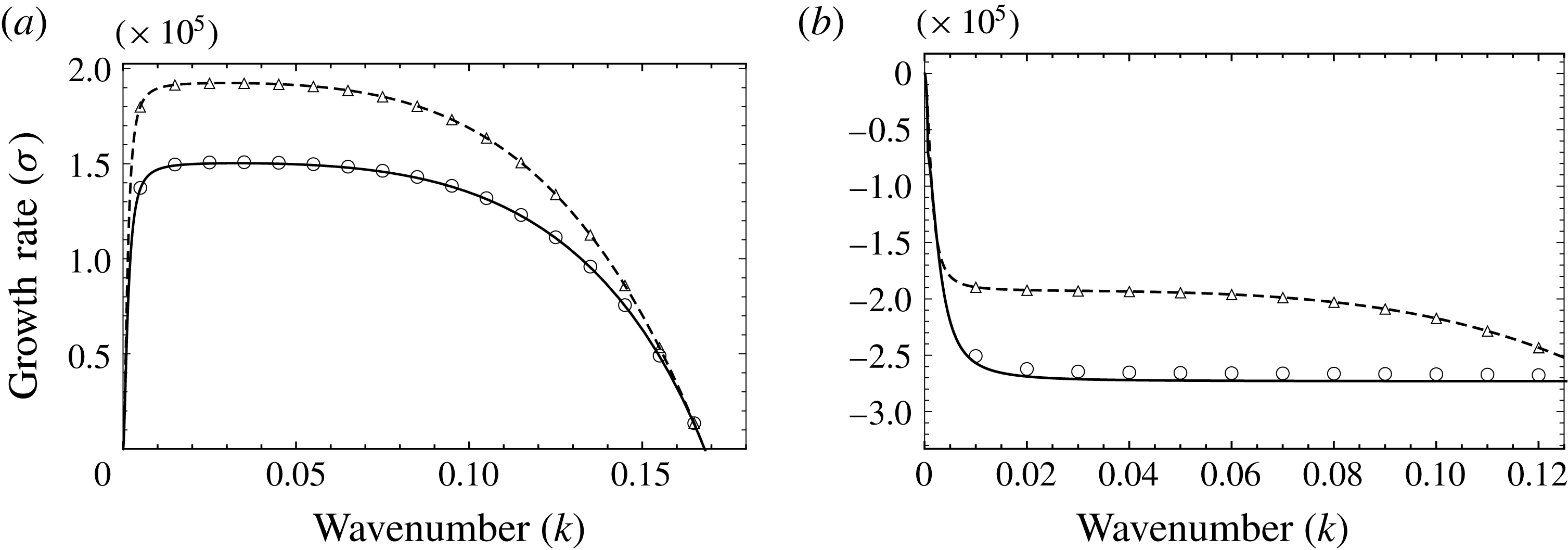
Growth rate versus wavenumber for evaporative instability without momentum inertia (dashed curve, triangles) and with momentum inertia (solid curve, circles);
 $H=0.3$
. The curves denote the growth rates obtained by linearizing the evolution equations (2.26) and the markers correspond to the growth rates obtained by linearizing the starting long-wave equations (2.2)–(2.14). (a) System is heated from the liquid side,
 $E=-6.1\times 10^{-5}$
. (b) System is heated from the vapour side,
 $E=6.1\times 10^{-5}$
. Momentum inertia has a stabilizing effect.
We now investigate the role of momentum and thermal inertia in the instability. Toward this, we introduce each inertial effect one after the other to single out the physics associated with them. First, we introduce momentum inertia alone into the problem by retaining Reynolds number but in the limit of vanishing Prandtl numbers (
 $Pr_{i}\rightarrow 0$
). The results of linear stability analysis for this case are plotted in figure 10. The curves represent the results obtained by linearizing the WRIBL model (2.26) and the markers denote the growth rates calculated by linearizing the starting long-wave equations (2.2)–(2.14). It can be seen that both are in excellent agreement. As evident from the figure, the growth rates associated with the long-wave instability are lower in the presence of momentum inertia, when heated from either liquid or vapour side. Also, the neutral wavenumber corresponding to zero growth rate remains unaffected (cf. figure 10
a), because the base state velocity is zero. The nonlinear evolution of the interface is found to be qualitatively similar to the creeping flow limit depicted in figures 4 and 5. The only difference being that the interface evolves at a slower rate resulting in a longer rupture time. The stabilizing effect of momentum inertia is attributed to the domain transients of velocity fields. Momentum inertia causes a delay in the response of a fluid parcel within the domain to any interface deformation as opposed to the creeping flow limit where the flow is adiabatically slaved to interface deformation.
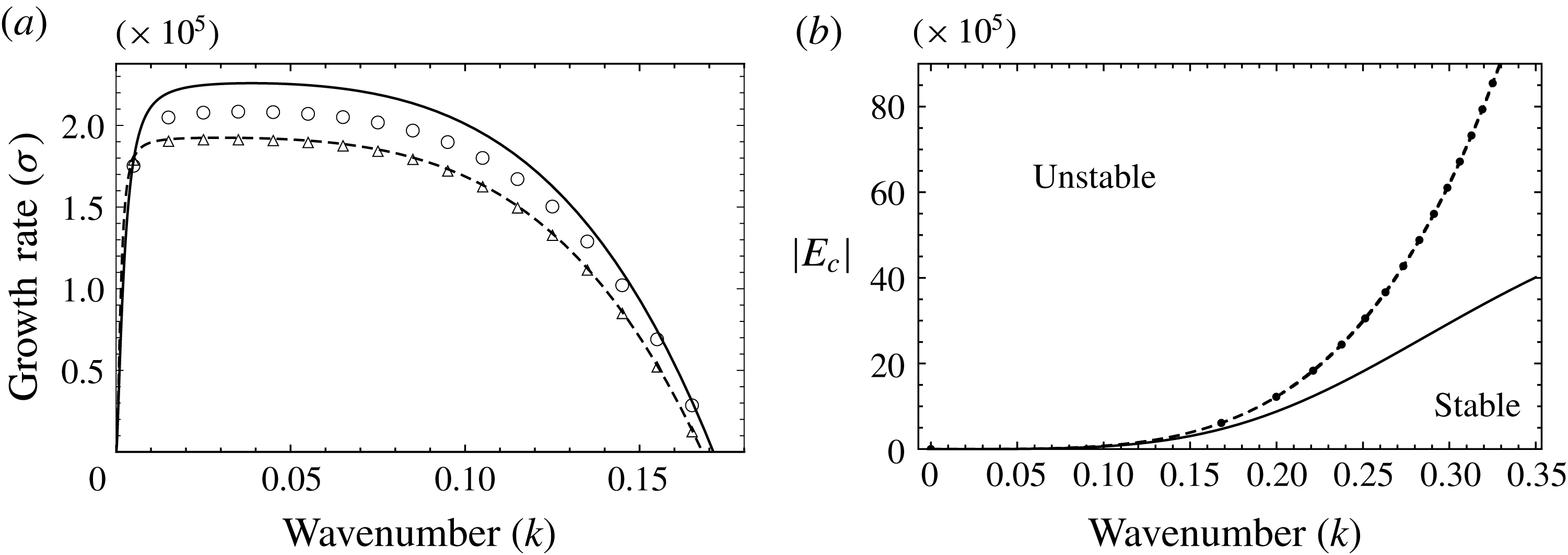
(a) Growth rate versus wavenumber for evaporative instability without thermal inertia (dashed curve, triangles) and with thermal inertia (solid curve, circles). The curves denote the growth rates obtained by linearizing the evolution equations (2.26) and the markers correspond to the growth rates obtained by linearizing the starting long-wave equations (2.2)–(2.14). System is heated from the liquid side;
 $E=-6.1\times 10^{-5}$
,
 $H=0.3$
. Thermal inertia has a destabilizing effect. (b) Neutral curve corresponding to instability threshold; dashed line: creeping flow limit, dots: effect of momentum inertia, solid line: effect of thermal inertia.
We next investigate the role of thermal inertia in the instability mechanism. Both Reynolds and Prandtl numbers are taken to be finite. However, we drop the terms associated with momentum inertia (left-hand sides of (2.26b
) and (2.26c
)) in order to selectively incorporate the effects of thermal inertia alone into the problem. The linear growth rates as a function of wavenumber when heated from the liquid side are plotted in figure 11(a). It is observed that the growth rates are higher in the presence of thermal inertia. Though the growth rates of the WRIBL model (curves) are slightly off compared to the starting long-wave equations (markers), the neutral wavenumber corresponding to the instability threshold is exactly captured. This is because the leading-order temperature profile assumption is not valid far away from the threshold. In appendix E, we show that the accuracy of the WRIBL model can be improved by considering a higher degree polynomial description for the leading-order temperature profile. Moreover, as the magnitude of the evaporation number (
 $|E|$
) is reduced, the WRIBL model and the complete long-wave model get very close to one another. It might also be noted that the WRIBL model with linear temperature profile is able to capture the essential destabilizing effects of thermal inertia and the reader will see that it is an excellent approximation when the system is heated from the vapour side, a case of interest, in § 3.2. The neutral wavenumber is found to increase from the case where thermal inertia is ignored. This suggests a destabilizing effect of thermal inertia on the system. The effect of thermal inertia is clearer from figure 11(b), where we have plotted the magnitude of the critical evaporation number (denoted by
 $|E_{c}|$
) corresponding to the onset of instability as a function of the wavenumber. The dashed line denotes the creeping flow limit. The dots and the solid line reflect the effect of momentum inertia and thermal inertia respectively. The region above the curve is unstable and that below the curve, stable. As discussed earlier and now evident from figure 11(b), momentum inertia does not affect the neutral wavenumber. However, the presence of thermal inertia lowers the magnitude of
 $E_{c}$
corresponding to the onset of instability, once again indicating that thermal inertia destabilizes.
The destabilizing effect of thermal inertia is explained as follows. In the creeping flow limit, the temperature profile,
 $T_{i}$
is slaved to the interface position,
 $h(x,t)$
. However, thermal inertia, when included, eliminates this slaved evolution of the temperature profile within each phase and the temperature profiles are further modified by thermal convection induced by flow. The convective transport of heat due to the flow results in a larger imbalance of conductive heat flux at the interface, resulting in a larger evaporative mass flux. This is depicted in figure 12, where the net mass flux,
 $J_{net}$
, is plotted with time for both creeping flow (dashed curve) as well as in the presence of thermal inertia (solid curve). The net mass flux,
 $J_{net}$
, is defined as below
 $$\begin{eqnarray}J_{net}=\sqrt{\int _{0}^{L}(J^{2})\,\text{d}x}.\end{eqnarray}$$
As seen from (3.3),
 $J_{net}$
is a measure of net phase change, including both evaporation and condensation, at the interface. Figure 12 shows that the presence of thermal inertia results in higher rates of phase change at the interface and thereby destabilizes the interface.
The nonlinear spatio-temporal evolution of the interface in the presence of thermal inertia exhibits qualitatively similar behaviour as in the creeping flow limit depicted in figures 4 and 5. The interface however evolves at a faster rate, thereby resulting in a shorter rupture time. This is evident from figure 12, where the rupture time corresponds roughly to the end of the curves. This is consistent with the higher linear growth rates observed in the presence of thermal inertia in figure 11(a).
The effect of thermal inertia on net mass flux undergoing phase change;
 $H=0.3$
,
 $E=-6.1\times 10^{-5}$
. Dashed line: creeping flow, solid line: with thermal inertia.

3.2 Rayleigh–Taylor problem in the presence of evaporation
Our principal interest in this section is on the effect of evaporation on an unstable liquid-above-vapour arrangement. However, let us first consider the case wherein the fluids are arranged in a light-over-heavy configuration. Gravity stabilizes the system. When heated from the vapour side, phase change also has a stabilizing effect and hence the system is always linearly stable. When heated from the liquid side, the system is unstable due to evaporative phase change. Gravity in this case then acts to reduce the range of unstable wavenumbers and mitigates the linear growth rates. The nonlinear interface evolution and rupture profiles are similar to that discussed in the previous section (in the absence of gravity) and therefore shall not be discussed here. In accordance with the linear theory, gravity also results in a delay in the nonlinear rupture time.
Now, focus on the case where the system is in a heavy-over-light configuration. In this case, the system is inherently unstable due to buoyancy-induced R–T instability. When heated from the liquid side, evaporation introduces added instability. We have learnt that the destabilizing effect of phase change becomes stronger as the interface approaches the heated wall. This is evident from figure 4(b), wherein the rate of interface deformation is seen to increase sharply with time as the interface approaches the wall. In contrast, for the R–T instability, the destabilizing effect of buoyancy is strongly damped by viscous forces near the wall and the rate of interface deformation decreases as the interface approaches the wall (cf. Lister et al. Reference Lister, Rallison and Rees2010). Therefore, for a R–T unstable system heated from the liquid side, the long-time interface dynamics is dominated by evaporation and the rupture dynamics is similar to that described for pure evaporation. The interface develops sharp crests (or troughs) that lead to rupture without sliding or cascade of buckling events. When heated from the vapour side, phase change counteracts the destabilizing R–T instability. As pointed out earlier, this was observed by several earlier workers (Hsieh Reference Hsieh1978; Ho Reference Ho1980; Adham-Khodaparast et al. Reference Adham-Khodaparast, Kawaji and Antar1995; Kanatani Reference Kanatani2010). In the following sub-sections, we discuss this case under various limits and make several new observations.
3.2.1 Inertialess creeping flow limit
(a) Growth rate versus wavenumber for R–T unstable configuration, heated from the vapour side. The curves denote the growth rates obtained from (3.1) and the markers correspond to the growth rates obtained by linearizing the starting long-wave equations (2.2)–(2.14).
 $E=1.22\times 10^{-4}$
(dashed, circles),
 $6.1\times 10^{-5}$
(dash-dotted, squares) and
 $1.22\times 10^{-5}$
(solid, triangles). The system is stabilized with increase in
 $E$
and is linearly stable for
 $E=1.22\times 10^{-4}$
. (b) Neutral curve corresponding to the division of stable (shaded) and unstable (unshaded) regions;
 $H=0.3$
.

(a) Steady-state interface profile for R–T unstable configuration, heated from the vapour side;
 $E=1.22\times 10^{-4}$
(dotted),
 $6.1\times 10^{-5}$
(dashed) and
 $1.22\times 10^{-5}$
(solid). (b) Temporal evolution of
 $h_{min}$
and
 $h_{max}$
corresponding to the unstable cases of
 $E=6.1\times 10^{-5}$
(dashed) and
 $1.22\times 10^{-5}$
(solid);
 $H=0.3$
,
 $k=0.2$
. Also cf. movies 4 and 5 for interface evolution.

(a) Initial velocity profile in each phase for the R–T unstable configuration, heated from the vapour side. (b) Velocity profile in each phase when the interface attains a steady configuration shows flow reversal in the liquid (also cf. movie 6). Only vector heads are plotted to indicate the direction of flow. Solid curve denotes the interface;
 $H=0.3$
,
 $E=2.44\times 10^{-5}$
,
 $k=0.2$
.

We first investigate the case where inertia is absent, inertia being taken into account in § 3.2.3. In figure 13(a), we have plotted the linear growth rates as a function of wavenumber for three different values of
 $\unicode[STIX]{x0394}T=10\,^{\circ }\text{C}$
,
 $5\,^{\circ }\text{C}$
and
 $1\,^{\circ }\text{C}$
, i.e.
 $E=1.22\times 10^{-4}$
,
 $6.1\times 10^{-5}$
and
 $1.22\times 10^{-5}$
. The curves correspond to the linearized evolution equations (2.26) and the markers denote the linearized starting long-wave equations (2.2)–(2.14). It can be seen from the panel that both of them are identical. Figure 13(a) shows that phase change stabilizes R–T configuration. With an increase in evaporation number, a decrease in both growth rates as well as the range of unstable wavenumbers is observed. This effect of phase change is depicted clearly in figure 13(b), wherein we have plotted the neutral curve corresponding to the division of stable (shaded) and unstable (unshaded) regions. It can be inferred from the figure that there exists a critical evaporation number (
 $E\approx 1.22\times 10^{-4}$
) that can linearly stabilize the system. This implies that a flat interface between a heavy-over-light fluid continues to remain so if
 $E$
exceeds this critical value. Importantly, it is seen that for weaker evaporation (see
 $E=6.1\times 10^{-5}$
and
 $E=1.22\times 10^{-5}$
in figure 13
a), two neutral points emerge. We contrast this with the case of Marangoni suppression of R–T instability (Alexeev & Oron Reference Alexeev and Oron2007) where only one bifurcation point is possible in appendix F. The bifurcation behaviour close to the two neutral points shall be analysed in the next section. For wavenumbers bounded by these two neutral wavenumbers, linear growth rates are positive suggesting that the interface is unstable and should undergo deformation, but not necessarily break-up. In figure 14(a), the steady-state interface profile for three values of evaporation number, viz.,
 $E=1.22\times 10^{-4}$
(dotted),
 $E=6.1\times 10^{-5}$
(dashed) and
 $E=1.22\times 10^{-5}$
(solid) are plotted. The fastest growing linear mode (
 $k=0.2$
) is chosen as the imposed perturbation. From figure 14(a), it can be seen that for the linearly stable case of
 $E=1.22\times 10^{-4}$
, the interface returns to its flat configuration. For
 $E=6.1\times 10^{-5}$
and
 $E=1.22\times 10^{-5}$
, although the system is linearly unstable, the interface nonlinearly saturates to a steady non-ruptured configuration. A decrease in evaporation (lower
 $E$
) causes the interface to saturate closer to the walls (cf. figure 14
b). The videos of the interface evolution corresponding to these two unstable cases of
 $E=6.1\times 10^{-5}$
and
 $E=1.22\times 10^{-5}$
are provided in the supplementary movies 4 and 5 respectively. Qualitatively, similar results were obtained using a one-sided model by Bestehorn & Merkt (Reference Bestehorn and Merkt2006) as well as by Kanatani & Oron (Reference Kanatani and Oron2011) using their two-sided model. In figures 15(a) and 15(b) respectively, we have plotted the the initial transient as well as the steady-state velocity profiles within each phase. It is interesting to note here that the velocity profile in the liquid phase in the initial stages is dominated by buoyancy (flow is from crest to trough). The vapour flow is from trough to crest. As the interface deforms due to buoyancy, the trough approaches the hot wall. This results in strong evaporation at the trough and generates a strong vapour flow due to the large density difference between the two phases. This vapour flow then eventually drags the liquid along with it, causing a flow reversal in the liquid phase opposing the effect of buoyancy (also cf. movie 6). This shear-induced flow reversal in the liquid phase by the evaporating vapour is the reason for saturation. One-sided evaporation models that do not account for an active vapour phase must therefore be more unstable. For negligibly low evaporation rates, it is found that the system behaviour resembles that of a pure R–T instability. The interface initially evolves as in figure 14(b). However, due to negligible evaporation, the interface continues to deform and saturated steady profiles are not obtained. Instead, the buckled interface exhibits sliding at very long times as the film approaches rupture, similar to that reported by Lister et al. (Reference Lister, Rallison and Rees2010) in the case of a pure R–T instability. The temporal evolution of the interface depicting sliding is shown in figure 16 for an initial hold-up of
 $H=0.8$
. It can be seen that the primary crest of the perturbed interface (dashed,
 $t=8.2\times 10^{5}$
) undergoes buckling as it approaches the wall (dot-dashed) at
 $t=8.2\times 10^{6}$
. This buckled profile of the interface is a quasi-steady configuration and it continues to evolve at extremely slow rates. At very long times (dashed,
 $t=3.1\times 10^{8}$
and solid,
 $t=3.7\times 10^{8}$
), the interface exhibits spontaneous sliding as was also shown by Lister et al. (Reference Lister, Rallison and Rees2010). In the next sub-section, we proceed to analyse the bifurcation behaviour of the two neutral points that we encountered in this sub-section.
Sliding of the interface as it nears rupture for very weak evaporation. The arrow indicates the direction of sliding. The profiles are plotted for
 $t=8.2\times 10^{5}$
(dotted),
 $t=8.2\times 10^{6}$
(dot-dashed),
 $t=3.1\times 10^{8}$
(dashed), and
 $t=3.7\times 10^{8}$
(solid);
 $H=0.8$
,
 $E=1.22\times 10^{-9}$
,
 $k=0.2$
.
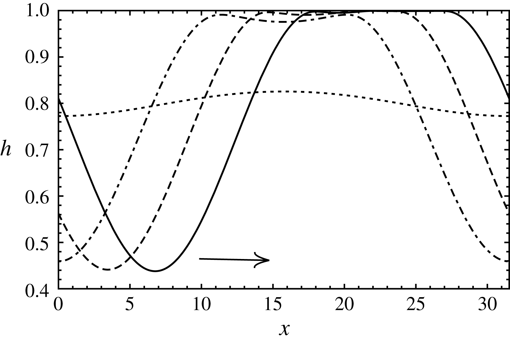
3.2.2 Bifurcation behaviour at the neutral points
In § 3.2.1, we saw that strong evaporation can linearly stabilize an interface which is otherwise R–T unstable. When evaporation was decreased just enough for gravitational effects to dominate, we saw the emergence of two neutral points that bound the unstable wavenumbers in figure 13(a). In this section, we evaluate the bifurcation behaviour at the two neutral points using a weak nonlinear analysis. The analysis is carried out in the limit of vanishing inertia (
 $Re\rightarrow 0$
). This is because the inertial effects are only expected to slightly alter the bifurcation points. The nature of bifurcation, however, is expected to remain the same. The control parameter,
 $G$
is advanced by a small amount from its critical threshold value, i.e.
 $G=G_{c}+(1/2)\unicode[STIX]{x1D6FF}^{2}$
, where
 $\unicode[STIX]{x1D6FF}$
is a small parameter that quantifies the distance from critical threshold value of the control parameter,
 $G_{c}$
. The variables are expanded as a regular perturbation series in
 $\unicode[STIX]{x1D6FF}$
. Solvability at third order is imposed to obtain an amplitude equation as given below:
 $$\begin{eqnarray}A-\unicode[STIX]{x1D701}\,A^{3}=0.\end{eqnarray}$$
Here,
 $A$
is the amplitude of the interface position. The details of the analysis are presented in appendix C. The bifurcation is supercritical when
 $\unicode[STIX]{x1D701}>0$
and subcritical if
 $\unicode[STIX]{x1D701}<0$
. A supercritical bifurcation indicates nonlinear saturation of the interface, whereas a subcritical bifurcation indicates the possibility of rupture. In our calculations, we choose
 $\unicode[STIX]{x1D6FF}=0.005$
and the value of
 $\unicode[STIX]{x1D701}$
is calculated numerically.
(a) Growth rate versus wavenumber for R–T unstable configuration when heated from the vapour side;
 $H=0.3$
,
 $E=1.1\times 10^{-4}$
. (b) Steady interface profile close to the left neutral wavenumber (
 $k=1.01\,k_{c,L}$
);
 $k_{c,L}=0.167$
. (c) Steady interface profile close to the right neutral wavenumber (
 $k=0.99\,k_{c,R}$
);
 $k_{c,R}=0.227$
.
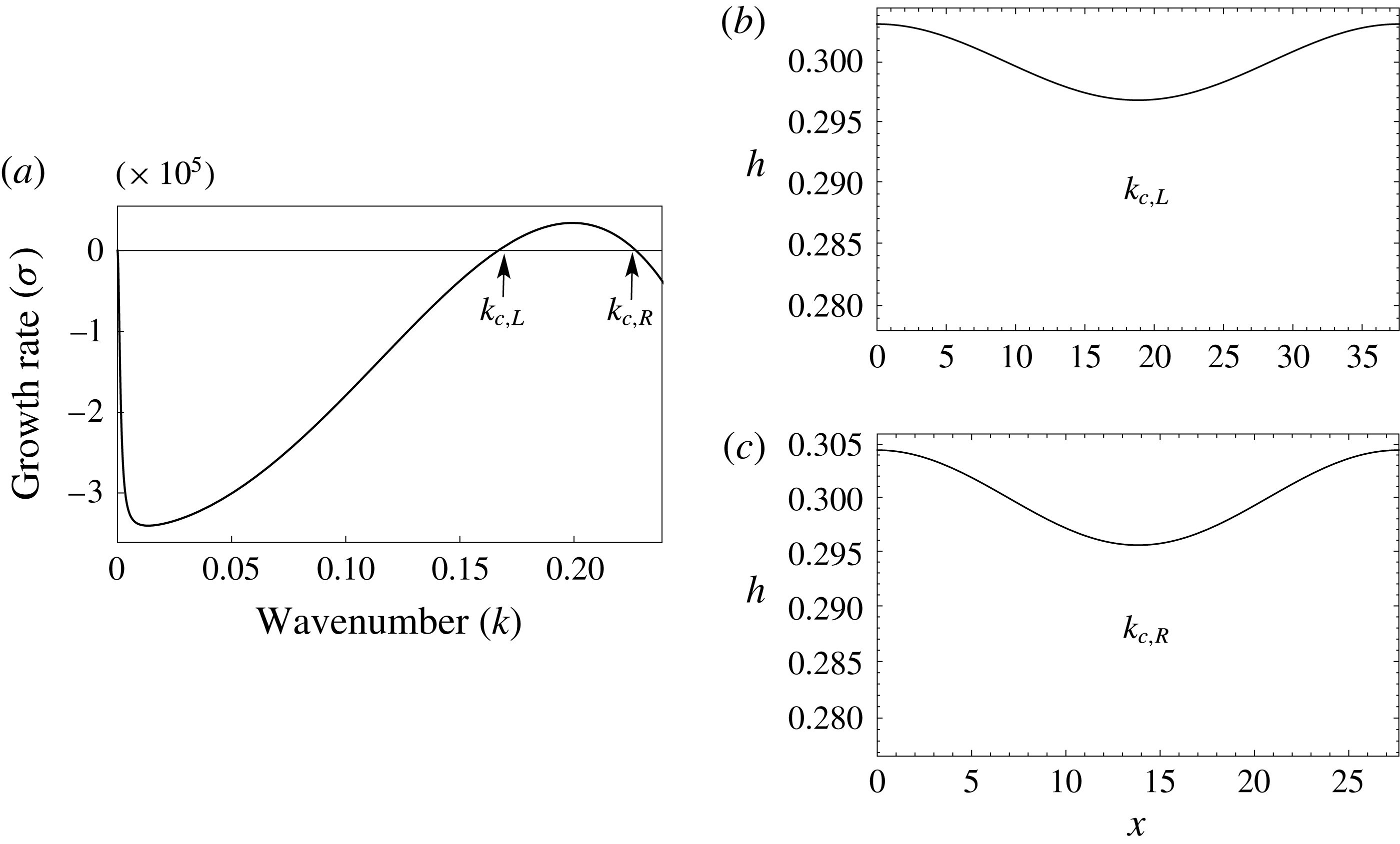
From figure 13(a), we know that for sufficiently strong evaporation
 $(E>1.22\times 10^{-4})$
, the linear growth rates are negative and the system is linearly stable. We now look at the case of
 $E=1.1\times 10^{-4}$
, wherein evaporation is strong but gravity just overcomes the effects of evaporation. The linear growth rate curve for this case is presented in figure 17(a) and it shows the emergence of two neutral points (denoted by
 $k_{c,L}$
and
 $k_{c,R}$
). The two neutral wavenumbers are closely spaced and the unstable wavenumbers are bounded between them. Our weak nonlinear calculations show that both these neutral wavenumbers are supercritical with
 $\unicode[STIX]{x1D701}>0$
. The nonlinear evolution of the interface corresponding to these two neutral wavenumbers is shown in figure 17(b,c). As expected from the weak nonlinear analysis, the interface saturates to a small amplitude cosine profile, indicating a supercritical bifurcation. Thus, the onset of instability results in similar interface profile irrespective of the choice of the neutral point.
Growth rate versus wavenumber for R–T unstable configuration when heated from the vapour side;
 $H=0.3$
,
 $E=3.66\times 10^{-5}$
. (b) Steady interface profile close to the left neutral wavenumber (
 $k=1.01\,k_{c,L}$
);
 $k_{c,L}=0.081$
(cf. movie 7). (c) Steady interface profile close to the right neutral wavenumber (
 $k=0.99\,k_{c,R}$
;
 $k_{c,R}=0.269$
).

Growth rate versus wavenumber for R–T unstable configuration when heated from the vapour side;
 $H=0.3$
,
 $E=1.22\times 10^{-11}$
. (b) Interface approaches rupture close to the right neutral wavenumber (
 $k=0.99\,k_{c,R}$
),
 $k_{c,R}=0.282$
.

Next, we look at the case of
 $E=3.66\times 10^{-5}$
, where evaporation is further reduced and the neutral wavenumbers are far apart. Figure 18(a) shows the linear growth rate curve for this case. It will be shown that this particular case is chosen for good reason. Here, the range of unstable wavenumbers bounded between the two neutral wavenumbers includes the higher harmonics of
 $k_{c,L}$
. It is the presence of these higher unstable harmonics that will be shown to be of importance. Our weak nonlinear calculations show that the two neutral points are supercritical. Therefore the interface is expected to nonlinearly saturate and it does. In figure 18(b), the steady interface profile corresponding to the left neutral wavenumber (
 $k_{c,L}$
) shows nonlinear saturation of the interface. However, since the domain length corresponding to
 $k_{c,L}$
allows higher unstable harmonics such as
 $2k_{c,L}$
and
 $3k_{c,L}$
, the final steady profile is dominated by these higher harmonics. A video of the interface evolution for this case is shown in the supplementary movie 7. Figure 18(c) on the other hand shows that for
 $k_{c,R}$
, the interface evolves to a small amplitude cosine profile as in the earlier case. This is because all higher harmonics of
 $k_{c,R}$
are stable with negative growth rates. Thus, depending on the choice of the critical domain size, the onset of instability can result in two very distinct interface profiles.
Our calculations suggest that
 $k_{c,L}$
remains supercritical for further decrease in
 $E$
and below a critical evaporation number,
 $k_{c,L}$
disappears and the system has only one neutral wavenumber,
 $k_{c,R}$
. At this value of
 $E$
,
 $k_{c,R}$
is still supercritical. With further decrease in
 $E$
, the neutral wavenumber,
 $k_{c,R}$
then approaches the pure R–T neutral point and
 $k_{c,R}$
turns subcritical with
 $\unicode[STIX]{x1D701}<0$
. In figure 19(a), we have plotted the linear growth rate curve for such a case. As seen from the panel, there exists only one neutral wavenumber
 $k_{c,R}$
. The linear growth rate curve matches exactly with the pure R–T instability. In figure 19(b), it can be seen that unlike earlier cases where the interface showed saturation, here the interface profile evolves towards rupture indicating a subcritical bifurcation. The calculations depicted in the figure were stopped when the interface position reached 0.001 as significantly high spatio-temporal resolution is required for the simulation to continue beyond. If the calculations were to be continued, the interface is expected to buckle and exhibit sliding. In fact, for the case of
 $k=0.9k_{c,R}$
, it was verified that buckling followed by sliding occurred. We next investigate the role of inertia in the evaporative suppression of R–T instability. It should be noted here that the fastest growing linear mode is quite far away from the instability threshold. Our computations have shown that the fastest growing linear mode, as it is quite far from the instability threshold, exhibits sliding and associated rupture before
 $k_{c,R}$
turns subcritical. Therefore, in a practical experiment where all unstable wavenumbers are present, nonlinear saturated states are guaranteed when both neutral wavenumbers (
 $k_{c,L}$
and
 $k_{c,R}$
) are supercritical.
3.2.3 Effect of inertia in a R–T unstable system, heated from the vapour side
Effect of momentum and thermal inertia on growth rate versus wavenumber for a R–T unstable system, heated from the vapour side. The curves denote WRIBL model and the markers denote the long-wave equations. Dashed curve or circles denote creeping flow. Dot-dashed curve or triangles denote the effect of momentum inertia. Solid curve or squares denote the effect of thermal inertia.
 $H=0.3$
,
 $E=2.44\times 10^{-5}$
.

The results of linear stability analysis with inclusion of inertia are plotted in figure 20 for
 $\unicode[STIX]{x0394}T=2\,^{\circ }\text{C}$
, i.e.
 $E=2.44\times 10^{-5}$
. The curves denote the growth rates obtained by linearizing the evolution equations (2.26) and the markers correspond to the growth rates obtained by linearizing the starting long-wave equations (2.2)–(2.14). The dashed curve and circles denote creeping flow, dot-dashed curve and triangles denote the effect of momentum inertia, while the solid curve and squares denote the effect of thermal inertia. It is evident from the figure that the linear growth rates obtained from the WRIBL model are in good agreement with that of the starting long-wave equations. As shown earlier in the absence of gravity, momentum inertia lowers the linear growth rates. The effect of thermal inertia on the linear growth rates is almost negligible in figure 20. However, by artificially increasing the Prandtl numbers to larger values than in table 1, it was found that the linear growth rates increase similar to the results obtained in the absence of gravity. The results of nonlinear calculations for the fastest growing linear mode are depicted in figure 21. In figure 21(a), the temporal evolution of the minimum and maximum positions of the interface are plotted for creeping flow (dashed curves) as well as in the presence of momentum inertia (solid curves). It can be seen that the momentum inertia slows the rate of interface evolution consistent with its lower linear growth rates. Importantly, momentum inertia results in an oscillatory approach to the final steady configuration as shown in figure 21(a). The supplementary movie 8 shows a video of this oscillatory saturation of the interface. The interface finally attains the same steady non-ruptured configuration as in the creeping flow limit. It is interesting to note here that although the final non-ruptured configuration involves flow within each phase, momentum inertia does not affect the final steady interface configuration. This is attributed to the insignificant role played by the convective terms in momentum inertia as discussed earlier in § 3.1.2. Momentum inertia only affects the transient dynamics. A similar oscillatory saturation to a final steady state in the presence of momentum inertia has been observed by Smith & Vrane (Reference Smith, Vrane, Shyy and Narayanan1999), although for a different problem involving interface deformation of thin films driven by thermocapillarity. In figure 21(b), we have plotted the nonlinear time evolution of the minimum and maximum positions of the interface for creeping flow (dashed curves) as well as in the presence of thermal inertia (solid curves). We see that in the presence of thermal inertia, the interface undergoes larger deformation and settles to a steady configuration closer to the bottom wall. In the presence of thermal inertia, convective heat transfer modifies the temperature profile within each fluid domain. This, in effect, alters the normal gradients of temperature at the interface, thereby affecting the final non-ruptured state.
Temporal evolution of
 $h_{max}$
and
 $h_{min}$
for a R–T unstable system, heated from the vapour side. (a) Momentum inertia results in an oscillatory saturation (cf. movie 8). (b) Thermal inertia destabilizes and causes the interface to saturate closer to the wall. Dashed curves denote the evolution without inertia and the solid curves are with inertia;
 $H=0.3$
,
 $E=2.44\times 10^{-5}$
,
 $k=0.2$
.

4 Summary
A WRIBL model for a bilayer system undergoing phase change with inertial effects is developed. The model is valid for moderate Reynolds and Prandtl numbers. For pure evaporation, it is shown that phase change can cause the bilayer system to become unstable when heated from the liquid side. This evaporative instability may result in rupture of either the liquid or vapour layer to form drops or bubbles depending on system parameters such as vapour–liquid depth ratio. The interface evolution leading to rupture is shown to be different from Marangoni or R–T instability. Neither sliding nor a cascade of buckling events is observed. An enhanced rate of phase change as the interface approaches the wall results in the formation of ever-steepening crests (or troughs) that result in rupture. The role of inertia can be summarized as: (i) momentum inertia has a stabilizing effect, and (ii) thermal inertia has a destabilizing effect. When gravity is included, a R–T unstable configuration can be stabilized by phase change when heated from the vapour side. Strong evaporation linearly stabilizes the R–T instability. As evaporation is decreased, two neutral wavenumbers emanate which are found to be supercritical from a weak nonlinear analysis and the interface evolves to a non-ruptured steady state. The steady state is found to be a consequence of shear-induced flow reversal in the liquid due to strong vapour flow generated by evaporation. Inclusion of momentum inertia results in a slower and oscillatory saturation to the same unruptured steady state as in the creeping flow limit. Thermal inertia, however, results in a larger deformation of the interface and the steady non-ruptured interface shifts closer to the wall. As evaporation is reduced further, one of the neutral points disappears, while the other remains supercritical until it turns subcritical upon further reduction of evaporation. The interface evolution in this case resembles pure R–T instability (Lister et al. Reference Lister, Rallison and Rees2010) and shows spontaneous lateral sliding of the interface as it approaches the wall. As the fastest growing linear mode is quite far from the instability threshold, the interface may exhibit sliding before the second neutral wavenumber turns subcritical. Therefore, nonlinear saturated states are guaranteed in an experiment when both neutral wavenumbers are supercritical.
Acknowledgements
We thank J. R. Picardo, G. F. Dietze and G. Labrosse for their valuable discussions and suggestions. R.N. is grateful to the Institute of Advanced Study-Durham University, UK for a fellowship. We are also grateful to NSF via NSF-0968313, for financial support.
Supplementary material and movies
Supplementary material and movies are available at https://doi.org/10.1017/jfm.2018.714.
Appendix A. Linear approximation to Clausius–Clapeyron equation
In this appendix, we discuss how the linear Clausius–Clapeyron parameter,
 $S$
was determined for water–water vapour system. The Clausius–Clapeyron equation is given as
 $$\begin{eqnarray}\log \,\frac{P_{1}}{P_{2}}=\frac{\unicode[STIX]{x0394}\,H_{vap}}{R}\left(\frac{1}{T_{2}}-\frac{1}{T_{1}}\right).\end{eqnarray}$$
In the above, the gas constant,
 $R=8.314~\text{J}~\text{mol}^{-1}~\text{K}^{-1}$
,
 $\unicode[STIX]{x0394}\,H_{vap}=40.7~\text{kJ}~\text{mol}^{-1}$
,
 $P_{1}=101\,325~\text{Pa}$
and
 $T_{1}=373.15~\text{K}$
. Saturation pressure as a function of temperature obtained from (A 1) is depicted in figure 22 (denoted by markers). A linear approximation with a R-squared value of 0.993 is shown by the solid line and the corresponding equation is:
 $$\begin{eqnarray}P_{sat}=3637.3\,T-1.2\times 10^{6}.\end{eqnarray}$$
The slope of the curve (A 2) gives the linear Clausius–Clapeyron parameter,
 $S=3637.3$
.
Saturation pressure as a function of temperature for water–water vapour system as obtained from the Clausius–Clapeyron equation (solid markers) and its linear approximation (solid line) in the neighbourhood of 373.15 K and 1 atm.

Appendix B. Linear stability analysis
The coefficients,
 $\unicode[STIX]{x1D702}_{i}$
, appearing in (3.1) are listed below:
 $$\begin{eqnarray}\displaystyle \unicode[STIX]{x1D702}_{1} & = & \displaystyle 3CaE(\!G(-H{\mathcal{K}}+H+{\mathcal{K}})^{2} (\!H^{4}(\unicode[STIX]{x1D707}^{2}+\unicode[STIX]{x1D707}(-4\unicode[STIX]{x1D70C}^{2}+6\unicode[STIX]{x1D70C}-4)+\unicode[STIX]{x1D70C}^{2})\nonumber\\ \displaystyle & & \displaystyle -\,4H^{3}\unicode[STIX]{x1D707}(\unicode[STIX]{x1D707}-\unicode[STIX]{x1D70C}^{2}+3\unicode[STIX]{x1D70C}-3)+6H^{2}\unicode[STIX]{x1D707}(\unicode[STIX]{x1D707}+\unicode[STIX]{x1D70C}-2)-4H(\unicode[STIX]{x1D707}-1)\unicode[STIX]{x1D707}+\unicode[STIX]{x1D707}^{2}\! )\nonumber\\ \displaystyle & & \displaystyle -\,\unicode[STIX]{x1D6F7}{\mathcal{K}}(\!H^{4}(\unicode[STIX]{x1D707}-1)(\unicode[STIX]{x1D707}-\unicode[STIX]{x1D70C})-2H^{3}\unicode[STIX]{x1D707}(2\unicode[STIX]{x1D707}+\unicode[STIX]{x1D70C}-3)+3H^{2}\unicode[STIX]{x1D707}(2\unicode[STIX]{x1D707}+\unicode[STIX]{x1D70C}-3)\nonumber\\ \displaystyle & & \displaystyle -\,4H(\unicode[STIX]{x1D707}-1)\unicode[STIX]{x1D707}+\unicode[STIX]{x1D707}^{2} )\!)\end{eqnarray}$$
 $$\begin{eqnarray}\displaystyle \unicode[STIX]{x1D702}_{2} & = & \displaystyle -(H-1)^{2}(H({\mathcal{K}}-1)-{\mathcal{K}})(\!3E\unicode[STIX]{x1D707}(H({\mathcal{K}}-1)-{\mathcal{K}})\nonumber\\ \displaystyle & & \displaystyle \times \,(H^{2}(\unicode[STIX]{x1D707}+3\unicode[STIX]{x1D70C}-4)-2H(\unicode[STIX]{x1D707}-2)+\unicode[STIX]{x1D707})+\unicode[STIX]{x1D6F7}GCa(H-1)^{2}H^{4}(\unicode[STIX]{x1D70C}-1)\unicode[STIX]{x1D70C}\nonumber\\ \displaystyle & & \displaystyle \times \,(H(\unicode[STIX]{x1D707}-1)-\unicode[STIX]{x1D707})\!)\end{eqnarray}$$
 $$\begin{eqnarray}\displaystyle \unicode[STIX]{x1D702}_{3}=-\unicode[STIX]{x1D6F7}H^{4}\unicode[STIX]{x1D70C}(H-1)^{4}(H({\mathcal{K}}-1)-{\mathcal{K}})(H(\unicode[STIX]{x1D707}-1)-\unicode[STIX]{x1D707}) & & \displaystyle\end{eqnarray}$$
 $$\begin{eqnarray}\displaystyle \unicode[STIX]{x1D702}_{4}=36ECa\unicode[STIX]{x1D707}(\unicode[STIX]{x1D70C}-1)(-H{\mathcal{K}}+H+{\mathcal{K}})^{2}(H(\unicode[STIX]{x1D707}-1)-\unicode[STIX]{x1D707}) & & \displaystyle\end{eqnarray}$$
 $$\begin{eqnarray}\displaystyle \unicode[STIX]{x1D702}_{5} & = & \displaystyle 3Ca\unicode[STIX]{x1D6F7}(H-1)H\unicode[STIX]{x1D70C}(H({\mathcal{K}}-1)-{\mathcal{K}})\nonumber\\ \displaystyle & & \displaystyle \times \,(H^{4}(\unicode[STIX]{x1D707}-1)^{2}-4H^{3}(\unicode[STIX]{x1D707}-1)\unicode[STIX]{x1D707}+6H^{2}(\unicode[STIX]{x1D707}-1)\unicode[STIX]{x1D707}-4H(\unicode[STIX]{x1D707}-1)\unicode[STIX]{x1D707}+\unicode[STIX]{x1D707}^{2}).\qquad\end{eqnarray}$$
Appendix C. Weak nonlinear analysis
This appendix discusses the details pertaining to the weak nonlinear analysis carried out in § 3.2.2. We choose
 $G$
to be the control parameter. The bifurcation is conjectured to be a pitchfork and the control parameter is advanced from its critical value,
 $G_{c}$
, by an amount
 $(1/2)\unicode[STIX]{x1D6FF}^{2}$
, i.e.
 $G=G_{c}+(1/2)\unicode[STIX]{x1D6FF}^{2}$
. In response, the variables
 $(h,q_{l},q_{v},\unicode[STIX]{x1D703})$
are assumed to be series expansions in
 $\unicode[STIX]{x1D6FF}$
as given below.
 $$\begin{eqnarray}\displaystyle & \displaystyle h(x)=H+\unicode[STIX]{x1D6FF}h_{1}(x)+\frac{\unicode[STIX]{x1D6FF}^{2}}{2}h_{2}(x)+\frac{\unicode[STIX]{x1D6FF}^{3}}{6}h_{3}(x)+\cdots \,. & \displaystyle\end{eqnarray}$$
 $$\begin{eqnarray}\displaystyle & \displaystyle q_{v}(x)=\unicode[STIX]{x1D6FF}q_{1}(x)+\frac{\unicode[STIX]{x1D6FF}^{2}}{2}q_{2}(x)+\frac{\unicode[STIX]{x1D6FF}^{3}}{6}q_{3}(x)+\cdots \,. & \displaystyle\end{eqnarray}$$
 $$\begin{eqnarray}\displaystyle & \displaystyle q_{l}(x)=\unicode[STIX]{x1D6FF}q_{1}^{\ast }(x)+\frac{\unicode[STIX]{x1D6FF}^{2}}{2}q_{2}^{\ast }(x)+\frac{\unicode[STIX]{x1D6FF}^{3}}{6}q_{3}^{\ast }(x)+\cdots \,. & \displaystyle\end{eqnarray}$$
 $$\begin{eqnarray}\displaystyle & \displaystyle \unicode[STIX]{x1D703}(x)=\unicode[STIX]{x1D703}_{0}+\unicode[STIX]{x1D6FF}\unicode[STIX]{x1D703}_{1}(x)+\frac{\unicode[STIX]{x1D6FF}^{2}}{2}\unicode[STIX]{x1D703}_{2}(x)+\frac{\unicode[STIX]{x1D6FF}^{3}}{6}\unicode[STIX]{x1D703}_{3}(x)+\cdots \,. & \displaystyle\end{eqnarray}$$
In the above, it is to be noted that
 $h(x)$
and
 $\unicode[STIX]{x1D703}(x)$
are surface variables, whereas the flow rates (
 $q_{l}$
and
 $q_{v}$
) are domain integral quantities. The relation between the perturbed flow rates (
 $q$
) and the horizontal velocity component (
 $u$
) at each order is as given below:
 $$\begin{eqnarray}q_{1}(x)=\int _{0}^{H}u_{1}\,\text{d}z,\quad q_{1}^{\ast }(x)=\int _{H}^{1}u_{1}^{\ast }\,\text{d}z\end{eqnarray}$$
 $$\begin{eqnarray}q_{2}(x)=\int _{0}^{H}u_{2}\,\text{d}z+h_{1}u_{1}|_{H},\quad q_{2}^{\ast }(x)=\int _{H}^{1}u_{2}^{\ast }\,\text{d}z-h_{1}u_{1}^{\ast }|_{H}\end{eqnarray}$$
 $$\begin{eqnarray}\displaystyle & \displaystyle q_{3}(x)=\int _{0}^{H}u_{3}\,\text{d}z+3h_{1}u_{2}|_{H}+3h_{2}u_{1}|_{H}+3h_{1}^{2}u_{1}|_{H} & \displaystyle\end{eqnarray}$$
 $$\begin{eqnarray}\displaystyle & \displaystyle q_{3}^{\ast }(x)=\int _{H}^{1}u_{3}^{\ast }\,\text{d}z-3h_{1}u_{2}^{\ast }|_{H}-3h_{2}u_{1}^{\ast }|_{H}-3h_{1}^{2}u_{1}^{\ast }|_{H}. & \displaystyle\end{eqnarray}$$
We substitute the expansions given by (C 1)–(C 4) into the nonlinear evolution equations (2.26) and solve order by order in
 $\unicode[STIX]{x1D6FF}$
. The analysis is carried out in the limit of vanishing inertia (
 $Re\rightarrow 0$
). At
 $O(\unicode[STIX]{x1D6FF})$
, the coefficients
 $h_{1},q_{1}$
,
 $q_{1}^{\ast }$
and
 $\unicode[STIX]{x1D703}_{1}$
are determined up to an arbitrary amplitude,
 $A$
. Our intention is to determine the amplitude
 $A$
. For this, we go to the next order, i.e. equations at
 $O(\unicode[STIX]{x1D6FF}^{2}/2)$
. At this order, it is observed that the inhomogeneous terms are multiples of
 $A^{2}$
and solvability is satisfied. This allows us to solve for
 $h_{2},q_{2}$
,
 $q_{2}^{\ast }$
and
 $\unicode[STIX]{x1D703}_{2}$
at this order in terms of
 $A^{2}$
. We then proceed to the next order, i.e.
 $O(\unicode[STIX]{x1D6FF}^{3}/6)$
, where solvability condition requires a balance between the terms containing
 $A^{3}$
and
 $A$
to give us the amplitude equation:
 $$\begin{eqnarray}A-\unicode[STIX]{x1D701}\,A^{3}=0.\end{eqnarray}$$
In the above,
 $\unicode[STIX]{x1D701}$
is the Landau constant and the bifurcation is supercritical when
 $\unicode[STIX]{x1D701}>0$
and subcritical for
 $\unicode[STIX]{x1D701}<0$
.
Appendix D. Lubrication model for Marangoni instability
This appendix discusses the lubrication model for a one-sided Marangoni problem. The interface evolution obtained from this model is shown in figure 6(b) while comparing the interface evolution toward rupture with that of pure evaporation instability. The schematic for pure one-sided Marangoni instability is shown in figure 23. The unperturbed liquid is of depth,
 $H$
, and maintained in contact with a hot wall at temperature,
 $T_{H}$
. The gas in contact with the liquid is assumed to be hydrodynamically passive and at a temperature,
 $T_{\infty }$
. At the interface, the heat transfer is given by Newton’s law of cooling as
 $$\begin{eqnarray}-{\mathcal{K}}_{l}\frac{\unicode[STIX]{x2202}T}{\unicode[STIX]{x2202}z}(h)=h_{tr}[T(h)-T_{\infty }].\end{eqnarray}$$
In the above,
 $h_{tr}$
and
 ${\mathcal{K}}_{l}$
are interfacial heat transfer coefficient and liquid thermal conductivity. Choosing the length, velocity and time scales to be
 $H$
,
 $\unicode[STIX]{x1D6FC}_{l}/H$
and
 $H^{2}/\unicode[STIX]{x1D6FC}_{l}$
, wherein
 $\unicode[STIX]{x1D6FC}_{l}$
is the liquid thermal diffusivity, and using the usual long-wave lubrication theory, the evolution equation for the interface can be easily derived as
 $$\begin{eqnarray}h_{t}=\left[\frac{Ma\,Bi\,h^{2}}{2}\frac{h_{x}}{(1+Bi\,h)^{2}}-\frac{h^{3}}{3}\left(\frac{h_{xxx}}{Ca}-Gh_{x}\right)\right]_{x}.\end{eqnarray}$$
In the above,
 $Ma=\unicode[STIX]{x1D6FE}_{T}\unicode[STIX]{x0394}\,TH/\unicode[STIX]{x1D707}_{l}\unicode[STIX]{x1D6FC}_{l}$
,
 $G=\unicode[STIX]{x1D70C}gH^{3}/\unicode[STIX]{x1D707}\unicode[STIX]{x1D6FC}_{l}$
,
 $Ca=\unicode[STIX]{x1D707}_{l}\unicode[STIX]{x1D6FC}_{l}/\unicode[STIX]{x1D6FE}\,H$
and
 $Bi=h_{tr}H/{\mathcal{K}}_{l}$
, where
 $\unicode[STIX]{x1D6FE}_{T}$
,
 $\unicode[STIX]{x0394}T$
,
 $\unicode[STIX]{x1D707}_{l}$
and
 $\unicode[STIX]{x1D6FE}$
, respectively denote the temperature sensitivity of surface tension, temperature difference between the wall and passive gas
 $(T_{H}-T_{\infty })$
, liquid dynamic viscosity and interfacial tension. For pure Marangoni instability,
 $G$
is set to zero. While plotting the interface shape in figure 6(b), we use a coordinate transformation given by
 $z\ast =((h-1)/h)z+1$
so that the liquid domain is transformed from
 $z=[0,h]$
to
 $z\ast =[1,h]$
. This transformation results in a vertically inverted plot that aids in easier visual comparison with the results of pure evaporation obtained in figure 5.
Schematic of pure one-sided Marangoni problem.

Appendix E. Improved WRIBL model with quadratic temperature and weight function
A particular limitation of the WRIBL model, while retaining thermal inertia, is the assumption for the form of the leading-order velocity (
 $\hat{u} _{i}$
) and temperature (
 $\hat{T}_{i}$
) profiles. In our work, we assume the leading-order velocity profile to be parabolic and the temperature profile to be linear. This assumption restricts the validity of the WRIBL model to conditions with moderate inertial effects. In the neighbourhood of the instability threshold (close to
 $k_{c}$
), the linear temperature profile is valid and hence the instability threshold is captured accurately by the WRIBL model. However, as we move far away from the instability threshold, the linear assumption for the temperature profiles ceases to be valid and the temperature profiles may become significantly nonlinear. This is evident from figure 24(a), wherein the temperature eigenfunction in the liquid phase at a crest obtained from the starting long-wave equations is plotted for
 $k=0.02$
, far away from the threshold (
 $k_{c}=0.171$
). It can be seen that the temperature profile deviates from linearity in this case. This explains the discrepancy in the linear growth rates obtained from the WRIBL model and the starting long-wave equations. The discrepancy in the growth rates due to the linear assumption for leading-order temperature can be rectified by improving the leading-order description of temperature. Toward this, we derived a WRIBL model by considering a quadratic functional form for the leading-order temperature profiles and taking the residual of the energy equation with the corresponding quadratic weight functions as detailed by Trevelyan & Kalliadasis (Reference Trevelyan and Kalliadasis2004). This procedure yields two equations governing the evolution of local average temperature in each phase (
 $\unicode[STIX]{x1D703}_{l}$
and
 $\unicode[STIX]{x1D703}_{v}$
) as compared to one surface temperature (
 $\unicode[STIX]{x1D703}$
) obtained in § 2.2. In figure 24(b), we have plotted the linear stability results so obtained and compared with that obtained in figure 11(a). It can be seen that the WRIBL model with quadratic temperature and weight functions is in good agreement with the starting long-wave equations. In principle, incorporating even higher degree polynomial description for temperature profiles and taking residuals with the corresponding higher degree weight functions continue to improve the accuracy as well as validity of the model to regimes with significant inertia. Pursuing this, of course, leads to a mathematically involved nonlinear model. We have not pursued nonlinear calculations for the quadratic model as part of the current work. This is because, we believe the WRIBL model with linear assumption is capable of capturing all the physics of the inertial effects such as (i) the destabilizing effect of thermal inertia in pure evaporation, (ii) the saturation of the interface closer to the bottom wall due to thermal inertia in evaporative suppression of R–T instability.
(a) The temperature eigenfunction in the liquid phase (solid) exhibits deviation from the linear profile. The dashed line depicts a straight line joining the interface temperature to the wall temperature. System is heated from the liquid side;
 $E=-6.1\times 10^{-5}$
,
 $H=0.3$
,
 $k=0.02$
. (b) Reproduction of figure 12(a) along with the linear stability results obtained by linearizing the WRIBL model with quadratic temperature and weight functions (dotted curve).

Appendix F. A note on suppression of R–T instability
In this appendix, we compare the difference in the suppression behaviour of R–T instability by evaporation with that of thermal Marangoni stresses. As observed from figure 13, the evaporative suppression of R–T instability may exhibit up to two neutral wavenumbers. However, in the Marangoni suppression of R–T instability, only one neutral wavenumber emerges for any value of imposed Marangoni number. This is because the destabilization offered by gravity in an R–T unstable configuration typically scales with wavenumber as
 $k^{2}$
. The stability offered by evaporation, however, has a very strong dependence on wavenumber (
 $k$
) close to
 $k=0$
and then more or less saturates with wavenumber until surface tension forces become important (cf. figure 3
b). This dependence on wavenumber is primarily due to the physics of evaporation. Phase change depends principally on the normal temperature gradients at the interface. The cause of evaporative stabilization is thus not sensitive to the lateral variations or the wavenumber of the perturbation. Therefore, when perturbed, the growth rate immediately reaches a non-zero value close to
 $k=0$
, which continues to remain independent of the wavenumber until surface tension effects dominate. This may also be inferred from (3.1), where
 $\unicode[STIX]{x1D702}_{4}$
is typically much less than
 $\unicode[STIX]{x1D702}_{5}$
. Therefore, for small
 $k^{2}$
, the linear growth rate (
 $\unicode[STIX]{x1D70E}$
) is given approximately by
 $\unicode[STIX]{x1D70E}\sim \unicode[STIX]{x1D702}_{1}/\unicode[STIX]{x1D702}_{5}$
. This is also evident from figure 25(a), where we have plotted this approximate value of growth rate along with that obtained from (3.1), when heated from the vapour side. Thermocapillarity, on the other hand, is primarily driven by lateral variations of temperature along the interface. The stability offered by thermocapillarity, therefore is always dependent on the perturbation wavenumber and scales as
 $k^{2}$
(cf. Alexeev & Oron (Reference Alexeev and Oron2007)). The similar dependence of destabilizing effect of gravity and stabilizing effect of thermocapillarity on wavenumber (as
 $k^{2}$
) results in a monotonic decrease of the neutral wavenumber from
 $k_{c,RT}$
to
 $k_{c}=0$
with
 $Ma$
, beyond which the system becomes linearly stable. This is evident from figure 25(b), where the results of Marangoni suppression of R–T instability from model equation (D 2) are plotted.
(a) Linear growth rate for evaporation heated from vapour side (solid line), dashed line represents the approximate growth rate given by
 $\unicode[STIX]{x1D702}_{1}/\unicode[STIX]{x1D702}_{5}$
;
 $E=6.1\times 10^{-5}$
,
 $H=0.3$
. (b) Marangoni suppression of R–T instability. Only one neutral wavenumber exists for any value of
 $Ma$
. Pure R–T with
 $Ma=0$
(solid line),
 $Ma=-2.02\times 10^{-4}$
(dashed),
 $Ma=-6.08\times 10^{-5}$
(dash-dotted) and
 $Ma=-1.21\times 10^{-5}$
(dotted);
 $Ca=23\,854$
,
 $G=1.7\times 10^{-6}$
,
 $Bi=0.2$
.



