2.1. Characterizations

The terms “approximation” and “idealization” are applied to a wide range of activities and structures in science. Sometimes the two terms are carefully distinguished, as in Frigg and Hartmann (Reference Frigg, Hartmann and Zalta2009, sec. 1.1). Other accounts dissect one term, typically “idealization,” into types. McMullin (Reference McMullin1985) distinguishes six types of idealization, and Weisberg (Reference Weisberg2007) finds three. More commonly, the terms are used fluidly, without much discipline, and even interchangeably.Footnote ¹

My concern here is not the lexicographic task of discerning precisely how the terms are currently used. That would lead to an unproductive profusion of competing meanings. Rather, my concern is to identify an important division in the range covered by the terms. Do they involve novel reference? Whether they do will prove important to their roles in theorizing in the applications below. As a terminological convenience for the remainder of this article, I will stipulate characterizations of the two terms that indicate this division and, I hope, reflect more or less common usages:Footnote ²

These are not definitions; they merely specify important properties. They neglect pragmatic considerations often deemed essential, such as the simplicity of the description or the intelligibility of the idealizing system. However, they assert the distinction that will drive the remainder of the discussion: only idealizations introduce reference to a novel system.

The characterizations do not and need not identify how inexact a description may become before we cease to admit it as an approximation. It is unlikely that there is a single standard applicable to all cases. In one context, a mere 10% error may betoken a good approximation; in another, it may be an egregious mismatch. It is assumed that there is some standard of admissible inexactness for each target system, even if vague. All that matters for the analysis here is that, for some specific target system, the same standard is used for both approximations and idealization. An elaboration of the specific standard is not needed.

The characterization does not specify which properties of the idealizing system are invoked, for that is decided by the application at hand. In differing applications, a system may or may not function as an idealization according to the properties invoked. A clay brick may be an idealizing system for a wooden block in relation to how it stacks, but it may fail to be an idealizing system in relation to how it floats in water.

The characterization of idealizations is quite permissive when it comes to the nature of the idealizing system. They may be other real systems or fictitious systems or mathematical objects or even parts of the target system itself.Footnote ³ For present purposes, this level of permissiveness is acceptable. All these types of systems can do what is needed: provide descriptions of properties that are approximations of the target system. What follows will not depend on the nature of the idealizing systems. It will depend on whether they can exist at all or, if they do, whether they have the properties intended.

2.2. Examples

The differences between the two terms can be illustrated with the example of a body of unit mass falling in a weakly resisting medium. Its speed at time t is given by

where g is the acceleration due to gravity and k is a friction coefficient. Its speed when falling from rest at is

When the friction coefficient k is small, the speed of fall in the early stages is described nearly exactly by the first term in the power series:

This inexact description is an approximation of the fall. We can promote this approximation to an idealization by introducing reference to a fictional system, a mass of the same size falling under the same gravity in a vacuum. This idealizing system's fall is described exactly by , and this property provides an inexact description of the target system.

A second example foreshadows the problems to come. A colony of bacteria numbers at time t. Since the population will keep doubling in the same time unit under favorable conditions, its growth is often described by an exponential law

for some constant k. The law is an inexact description since must always be a whole number, and will almost never be so. However, the fractional error becomes smaller as the number of bacteria increases, and the law becomes a better approximation.

One might imagine in this last example that one can promote the approximation to an idealization by just “taking the limit to infinity” and imagining a system of infinitely many bacteria as the idealizing system. The attempt fails. If is actually infinite, it can no longer enter into the exponential law, which would now merely assert “infinity = infinity.” It is an approximation that can be made more accurate without restriction by taking larger n, but taking the limit system of an actual infinity of bacteria does not yield the intended idealization.

2.3. Promotion and Demotion

Approximations and idealizations are interrelated in a way illustrated by these last two examples:

In the inverse promotion, we consider the target system to be one of a sequence of systems whose limit system is intended to be the idealizing system. The promotion fails if the sequence fails to have a limit system or has a limit system with unsuitable properties.

2.4. Other Applications

The distinction drawn here illuminates other debates in philosophy of science. Consider realist and antirealist responses to the pessimistic metainduction. According to it (Laudan Reference Laraudogoitia and Zalta1981), history of science is replete with theories that are proven to be referential failures when an antecedent theory is replaced by a contradicting successor. In spite of its theory's successes in the late eighteenth and early nineteenth centuries, there is no caloric. So we should not expect referential success of our present theories.

Antirealists affirm this conclusion. They regard the antecedent theories (and probably the successors also) as inexact descriptions without referential success; they are all mere approximations. Realists, however, regard the antecedent theory as an idealization of the successor theory. It is referentially successful in that the idealizing system is a part of the same system the successor theory describes. The “caloric” of caloric theory refers to the same thing as the “heat” of thermodynamics but in the confines of situations in which there is no interchange of heat and work.Footnote ⁴

3.1. Limit Property and Limit System Agree

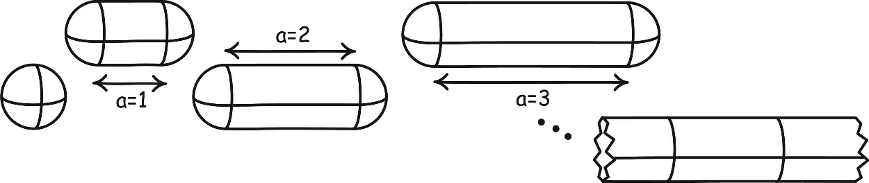
Consider a sphere of unit radius. It is elongated into a capsule, a cylinder with spherical end caps, as shown in figure 1. Its total length grows through the sequence of cylinder lengths a = 1, 2, 3, 4, … .

Figure 1.

Sphere elongated as capsule.

In the infinite limit, the capsule becomes an infinite cylinder of unit radius. The surface area of a capsule of cylinder length a is , and its volume is . Hence, the ratio of surface area to volume is , and the ratio approaches a limiting value of 2 as a goes to infinity. This limit of the properties of the sequence of capsules agrees with the corresponding properties of the limiting system, the infinite cylinder, whose ratio of area to volume is also 2.Footnote ⁵

The example implements the general scheme in which we have the sequences:

And the two cohere in that the limit property is the corresponding property of the limit system. Hence, the infinite cylinder is an idealization of the larger capsules.

3.2. There Is No Limit System

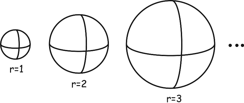
Consider a unit sphere whose radius r grows as r = 1, 2, 3, … , as shown in figure 2. The area of the sphere is 4πr ², and its volume is . The ratio of surface area to volume is , and this ratio goes to zero as the radius r goes to infinity. Hence, the sequence of properties has a limiting value. The sequence of systems, that is, of spheres, however, has no limit system. One might casually speak of “an infinitely large sphere” as the limit system. But that talk is literally nonsense. A sphere is the set of points equally far away from some center. An infinitely large sphere would consist of points infinitely far away from the center. But there are no such points. All points in the space are some finite distance from the center.

Figure 2.

Sphere expands uniformly.

This example implements the scheme

There is a limit property, but it is not a property of a limit system since there is none. The zero area-to-volume ratio is not a property of an impossible infinite sphere. It is a property of the set of all finite spheres; it is the greatest lower bound of the ratios of the set's members.

In this case, the limit property is an approximation, an inexact description, of the properties of the later members of the sequence of systems. However, the limit provides no idealization because there is no limit system to bear the limit property.

3.3. Limit Property and Limit System Disagree

Consider once again a sphere of unit radius. Uniformly expand it in one direction only, so it becomes an ellipsoid with semimajor axis a. Continue the expansion until a goes to infinity. The limit system is a cylinder of unit radius, as shown in figure 3.Footnote ⁶ The volume of the ellipsoid is . The surface area of the ellipsoid nears a value of , arbitrarily closely for large a. Hence, the ratio of surface area to volume approaches as a goes to infinity. This limit ratio is not the same as the corresponding ratio of 2 for the limit system, an infinite cylinder.

Figure 3.

Sphere elongated as ellipsoid.

The example implements the general scheme in which we have the sequences:

where the limit property is not a property of the limit system. This limit can be used to provide an approximation of the systems leading up to the limit. The limiting ratio of 3π/4 is a close approximation of the area-to-volume ratio of the very large ellipsoids. However, the limit does not provide an idealization. An infinite cylinder has an area-to-volume ratio of 2, which is a poor approximation of the ratio for large ellipsoids.

4.1. Idealizations

The most common limit is the “thermodynamic limit” in which both the number of components n and the volume they occupy are taken to infinity in such a way that the ratio remains constant. At least some texts are clear that the system to be investigated is the limit system of an actual infinity of components. I will call this the “strong” form of the thermodynamic limit. Ruelle (Reference Ruelle2004, 2) writes, “The physical systems to which the thermodynamic formalism applies are idealized to be actually infinite, i.e. to fill (where in the usual world). This idealization is necessary because only infinite systems exhibit sharp phase transitions. Much of the thermodynamic formalism is concerned with the study of states of infinite systems.” What makes the transition to an infinity of components admissible is the assumption that the infinite systems will provide a good description of large but finite systems. Ruelle (Reference Ruelle1999/2007, 11) remarks, “if a system exhibits thermodynamic behavior the states defined by the ensemble averages for large … finite systems approach in some sense states of the corresponding infinite system.”

The hope expressed by Ruelle is that the limit property and limit system will agree as in the well-behaved case of section 3.1. Then the limit system provides an idealization in the sense defined here. The long-recognized difficulty is that the infinite systems often have properties very different from those of the finite system. That is, they exhibit the discord of the limit property and limit system of section 3.3, so that the limit does not provide an idealization.

The difficulty is well known. Lanford (Reference Lanford and Moser1975, sec. 4) describes an infinite system of hard spheres all of which are at rest until some moment of excitation, after which a disturbance propagates in “from infinity,” setting all but finitely many of the spheres into motion. The system manifests a violation of determinism and also a violation of the conservation of energy and momentum. This is an early contribution to the now flourishing literature on supertask systems. It describes how infinitely many particles in classical and, sometimes, relativistic physics can interact to produce analogous violations of determinism and the conservation of energy and momentum. For recent work, see Atkinson (Reference Atkinson2007) and Lee (Reference Lee2011), and for a survey, see Laraudogoitia (Reference Laudan2011).

A version of this supertask that is not driven by carefully tuned collisions is a chain of masses connected by Hooke's law springs as shown in figure 4. It is a simple model of a one-dimensional crystal. The appendix shows that an infinite chain of these masses can spontaneously excite, violating determinism and energy conservation, and sketches how similar pathologies may arise for other infinite systems governed by a dynamics that is well behaved when applied to systems of finitely many components.

Figure 4.

Masses and springs.

In these cases, the infinite limit system fails to provide an idealization, and we have a case of the limit property and limit system disagreeing, as in section 3.3. All the finite systems have the properties of determinism and energy conservation; hence, the limit properties are determinism and conservation. The infinite limit system, however, is indeterministic and nonconservative.

The remedy is to add further conditions. To exclude the indeterministic behavior of his system of hard spheres, Lanford (Reference Lanford and Moser1975, 54) imposes a boundary condition on solutions that limits the magnitude of changes in position of the spheres. Lanford and Lebowitz (Reference Lanford, Lebowitz and Moser1975) consider the time evolution of harmonic systems such as crystals, and one of their examples is the one-dimensional chain of masses and springs above (148–49). They do not discuss the indeterministic time evolution of this system and proceed to theorems that assert the uniqueness of time evolution. This uniqueness seems to depend on a condition that bounds the maximum magnitude of displacements and momenta of the masses. This condition is more readily apparent in simpler versions of the uniqueness theorems, such as in Lanford (Reference Lanford1968, 180, theorem 2.1), where the component positions are directly required to be bounded functions of time.

Lanford investigated infinite systems as “the only precise way of removing inessential complications due to boundary effects, etc.” (Reference Lanford and Moser1975, 17). Yet is it the presence of the finite boundary that prevents the unwanted disturbances propagating in “from infinity”? It would seem that the better strategy is to analyze finite but very large systems so that this essential boundary effect is preserved.

In sum, there is a real difficulty facing the use of the strong thermodynamic limit as an idealization. One cannot assume that the limit of well-behaved finite systems will be a well-behaved infinite system. The remedy involves a kind of reverse engineering. We know the properties of infinite systems that are pathological, so we seek to restrict the systems for which the thermodynamic limit is taken in such a way that the pathological properties are not manifested. This is a result of some importance, and we will return to it below in section 5.3. The finite systems control the infinite systems in the sense that, if there is a conflict, we modify the infinite systems to match the finite ones.

4.2. Approximations

Another type of limit used in thermodynamics cannot be used to create idealizations. Its limiting processes are beset with pathologies so that it either yields no limit system or yields one with properties unsuited for an idealization.

4.2.1. The Continuum Limit

In the continuum limit described by Compagner (Reference Compagner1989), the number of components n goes to infinity in such a way that the extensive magnitudes of the system, such as volume and energy, remain constant. If d is a parameter that measures the size of the individual components, this condition entails that nd ³ remains a nonzero constant, for nd ³ is proportional to the volume of the system occupied by matter. Similarly, Boltzmann's constant k goes to zero since nk remains a nonzero constant. For the mean energy of a mole of a monatomic gas, n = N, is given by , and this remains constant in the limit.Footnote ⁷

While many properties will approach well-behaved limits, the system itself has no well-defined limit state. One might imagine that the infinitely many, infinitely small components spread over a finite volume have become a uniform matter distribution. However, such a uniform distribution is not approached in the limit. To see why, imagine that the system consists of massive components that half fill the volume and that the matter density within the components is uniformly unity.Footnote ⁸ The occupied portions of the volume consist of many islands of matter, where the matter density is unity, and they float in a sea of emptiness, where the matter density is zero. As we approach the limit, the matter islands are divided into smaller islands. However, at no stage does the system consist of anything other than regions with matter density unity and regions with matter density zero. Hence, the density of matter at an arbitrary point in space may oscillate between 0 and 1 and not approach the limiting value 1/2 of the uniform matter distribution.

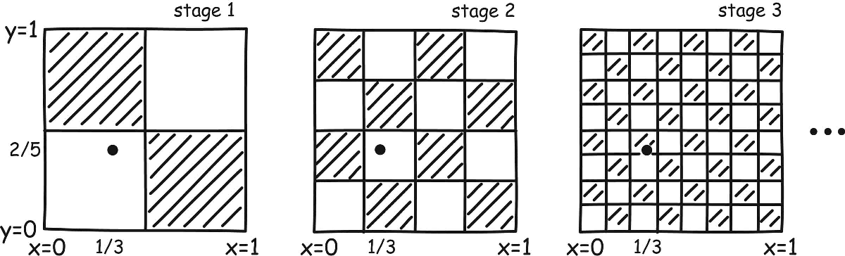
We can see the difficulty clearly in a simplified example. Consider a unit square that is divided into half, quarter, eighth squares, and so on, in stages 1, 2, 3, and so on, of a process as shown in figure 5. At each stage, half the squares are occupied—represented by shading—and half are not. The sequence mimics halftone printing, which simulates gray scales even though the printer can only assign either black or white to each point. Some points will approach limiting values. Points on the diagonal, such as (1/3, 1/3) will have the state “white” at all stages and thus carry “white” as a limiting value. Others will oscillate indefinitely. The states at the point (1/3, 2/5) shown in the figure will oscillate indefinitely as white, white, black, black, white, white, black, black, and so on, and thus admit no limiting value.Footnote ⁹ Hence, the limit will return points whose limiting color is black, points whose limiting color is white, and points with no limiting color. It does not yield a unit square uniformly covered in a 50% gray tone.

Figure 5.

Sequences in halftone printing.

It is the same with the continuum limit of a system of extended masses. There is no limit system in which the matter is somehow uniformly spread over the volume of space. The limit operation produces points that carry matter fully or not at all or have no limit state. We come close to the halftone-printing example if we consider the system of masses to be cooled to the absolute zero of temperature, so that the masses are at rest in an equilibrium configuration. If the resulting crystal is a cubic lattice, then the halftone printing analysis can be applied directly.

4.2.2. The Boltzmann-Grad Limit

A second example in which idealization fails is the Boltzmann-Grad limit taken in generating the Boltzmann equation (Lanford Reference Lanford and Moser1975, 70–89; Reference Lanford1981). The system consists of n hard spheres of diameter d. In the limit, n goes to infinity and d to zero in such a way that nd ² remains a nonzero constant. Since the volume of space occupied by matter varies with nd ³ = constant × d, the fraction of the volume of space occupied by matter drops to zero. Hence, the limit state consists of a countable infinity of extensionless points occupied by matter, and the rest of the volume of space is empty. Therefore, the limit state is not beset by a lack of convergence of the halftone printing problem, or at least the problem arises at worst in a measure zero set.

In the analysis leading up to the Boltzmann equation, the nonzero size of the bodies and their spherical shape determines whether two nominated bodies will collide and which will be the resulting motions. This resolution of collisions leads to the computation of the changes with time of the distribution of the spheres over the possible positions and velocities.

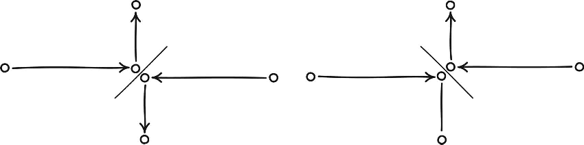
However, the limit state is too impoverished to support this computation. It now consists of an infinity of points of zero size in motion. If two points of the limit state collide (a measure zero event), we can no longer determine the collision outcome. We need to determine six quantities: three velocity components for each of the two outgoing points. We have only four equations: three for momentum conservation and one for energy conservation. Hence, any collision has become indeterministic. Until we reach this limit state, collision outcomes can be determined uniquely since we have the added condition that, when spheres collide, the momentum transfer is perpendicular to the plane of contact of the two sphere's surfaces, as shown in figure 6 (Lanford Reference Lanford and Moser1975, 8). Two colliding points no longer have a definite plane of contact.

Figure 6.

Resolving collisions.

Hence, neither continuum limit nor Boltzmann-Grad limit supports idealization. The first has no limit system, and the second has a limit system too impoverished to supply an inexact description of the finite systems.

4.3. Renormalization Group Methods Are Approximations Not Idealizations

The examples of the last two sections are less common. More commonly, when a limit to infinitely many components is considered, it is left unclear whether the limit is taken only for properties (approximation) or whether the limit system of an actual infinity of components is intended (idealization).

Some authors, such as Lanford and Ruelle, invoke the strong form of the thermodynamic limit and investigate the properties of infinite systems. Others use what I shall call a “weak” form of the thermodynamic limit that mentions only the existence of limit properties. Le Bellac, Mortessagne, and Batrouni (Reference Le Bellac, Mortessagne and Batrouni2004, 112) consider an extensive magnitude A(T, V, N), where T is the temperature, V the volume, and N the number of components. They consider the limit

where n = N/V is kept finite and, presumably, nonzero in the limit. The thermodynamic limit of A(T, V, N) is said to exist if a(n, T) is finite. Conspicuously absent is any condition on an actual infinity of components and the corresponding behavior of that infinite system.

Accounts of renormalization group methods routinely remark that the thermodynamic limit is essential for recovery of the discontinuities in thermodynamic quantities at critical points. Kadanoff (Reference Kadanoff2000, 239) reviews the governing fact that a partition function of a system of finitely many components is analytic. It becomes nonanalytic only in the limit of infinitely many components, whereupon the thermodynamic quantities derived from it can harbor discontinuities that characterize critical points. He continues: “We reach the important conclusion: The existence of a phase transition requires an infinite system. No phase transitions occur in systems with a finite number of degrees of freedom.” But which limit is actually used in the methods? Insofar as they yield results, we shall see the limit taken by renormalization group methods is of the properties only, such as in the weak thermodynamic limit of Le Bellac et al.

The methods are applied in a space of reduced Hamiltonians. To generate transformations between different Hamiltonians, we start with a thermal system with Hamiltonian H and suppress explicit dependence on some of the thermodynamic degrees of freedom to arrive at a new Hamiltonian H′. In “real space” renormalization, the components in space are collected into clusters, hiding the degrees of freedom in the clusters. Each is a component for a new Hamiltonian H′ of the same mathematical form as H but with different parameters. The clustering reduces the number of components from N to N′. If the dimension of the space is d, the two are related by

for some constant b. This transformation is only well defined if both N and N′ are finite. In momentum space renormalization, we Fourier transform our descriptions, replacing position variables by momentum variables. We “trace out,” that is, sum over and thus hide, the high-frequency (i.e., high-momentum) modes of the Hamiltonian H to arrive at the new H′.

The transformation of thermodynamic quantities is derived by recalling that the two Hamiltonians H and H′ are just different descriptions of the same system, so they must have the same total thermodynamic properties, such an energy, entropy, and free energy. Since total free energy , where Z(H) is the partition function derived from H, it follows that equality of total free energy of the two systems, , entails equality of the partition functions

Fisher (Reference Fisher and Hahne1982, 68) calls this essential equality “unitarity.”Footnote ¹⁰ The transformation of all thermodynamic quantities is derived from it. For example, the free energy f per component is given as , and the energy per component is given as . Hence, they transform as and as .

These derivations, in both real space and momentum space renormalization, depend essentially on the finitude of the system. The partition function of homogeneous systems of components is a product of many equal terms, one for each component. If the system consists of infinitely many components, then its partition function is zero or infinity, and unitarity will no longer induce nontrivial transformations.

The finite systems used to generate the transformations may be large subsystems of still larger finite systems or even subsystems of an infinite system, if one knows the infinite system's behavior is not pathological. But the Hamiltonians related by the transformations must describe finite systems, so that the Hamiltonians yield the finite, nonzero partition functions for a nondegenerate unitarity condition.

The renormalization group transformations induce a flow over the space of reduced Hamiltonians, and, for the reasons just given, this portion of the space must correspond to systems of finitely many components. Systems of infinitely many components at best enter as limit points of the flows since the transformations cannot map a finite system to an infinite system. They might correspond, for example, to the limit of the reversed sequence of transformations that undoes the suppression of component number degrees of freedom:

Critical points connected with infinitely many components appear in the diagrams of the space of reduced Hamiltonians (e.g., Fisher Reference Fisher and Hahne1982, 85). They are introduced as limit points that topologically close an open region of space filled with the renormalization group flow.

The methods do not directly compute the properties of systems of infinitely many components associated with the critical points. Rather, properties attributed to the critical points are just the limit properties of finite systems. Thus, we cannot take these critical points to represent an actually infinite system and their properties, for such systems may have properties very different from finite systems. They may, as we have seen, violate determinism and energy conservation, so that the whole framework of statistical physics would collapse. Without an analysis that precludes these anomalies, the points are best seen as mathematical artifices completing a diagram.

As an explanatory analogy, consider the space of all spheres. It is one-dimensional and coordinatized by the curvature (1/radius²). A map on the space expands and contracts the spheres; typical transformations would map spheres to others twice, thrice, and so on, their curvature. The resulting flow fills the portion of that space where curvature is greater than zero, as shown in figure 7. We close the space by adding the point at zero curvature, where a natural extension of the map has a fixed point. We might imagine that the added point represents a “sphere of zero curvature” and attribute limiting properties of finite spheres to it, such as the possession of a unique center and an inside and outside. However, there is no sphere of zero curvature. If the point represents anything at all, it represents an infinite Euclidean plane, which does not carry the sphere's limiting properties.

Figure 7.

Space of sphere curvature.

Critical points enter real space renormalization group methods as points in a diagram: mathematical pegs on which to hang limit properties. They do not arise from an investigation of the properties of infinite limit systems. They are not idealizations.

The acclaimed results of the methods pertain to critical exponents. For many systems, thermodynamic quantities at temperatures near the critical temperature turn out to be powers of the reduced temperature , commonly written as , , , and so on. Renormalization group methods have enjoyed great success in explaining universality: that very few numerical values of the critical exponents, α, β, γ, and so on, suffice for very many substances. The results are recovered by examining the renormalization group flow in the vicinity of the critical point. In this vicinity, the systems are finite, so that the results recovered apply to finite systems, albeit of arbitrarily large size. That is, insofar as limits enter, the results are recovered for limit properties, not limit systems, so that the acclaimed results concerning critical exponents are recovered by approximations.

5.1. Illustration of Nonanalyticity with Finite Systems

The most common argument in favor of the necessity of the infinite idealization is that infinite systems are needed if thermodynamic functions are to be nonanalytic and thus support the discontinuities of phase transition. The argument overstates what is needed. One does not need the limit system with an infinity of components. Consider the functional dependence of some property on the number of components n in a set of systems, all of which have a finite n. Taking the limit as n goes to infinity in this function, as a purely mathematical operation, can yield a nonanalytic function, without ever considering a system with an infinity of components. That nonanalytic function will be a very good approximation of the analytic functions of system of large, finite n. Butterfield (Reference Butterfield2011b) has described this effect with the slogan of “emergence before the limit.”

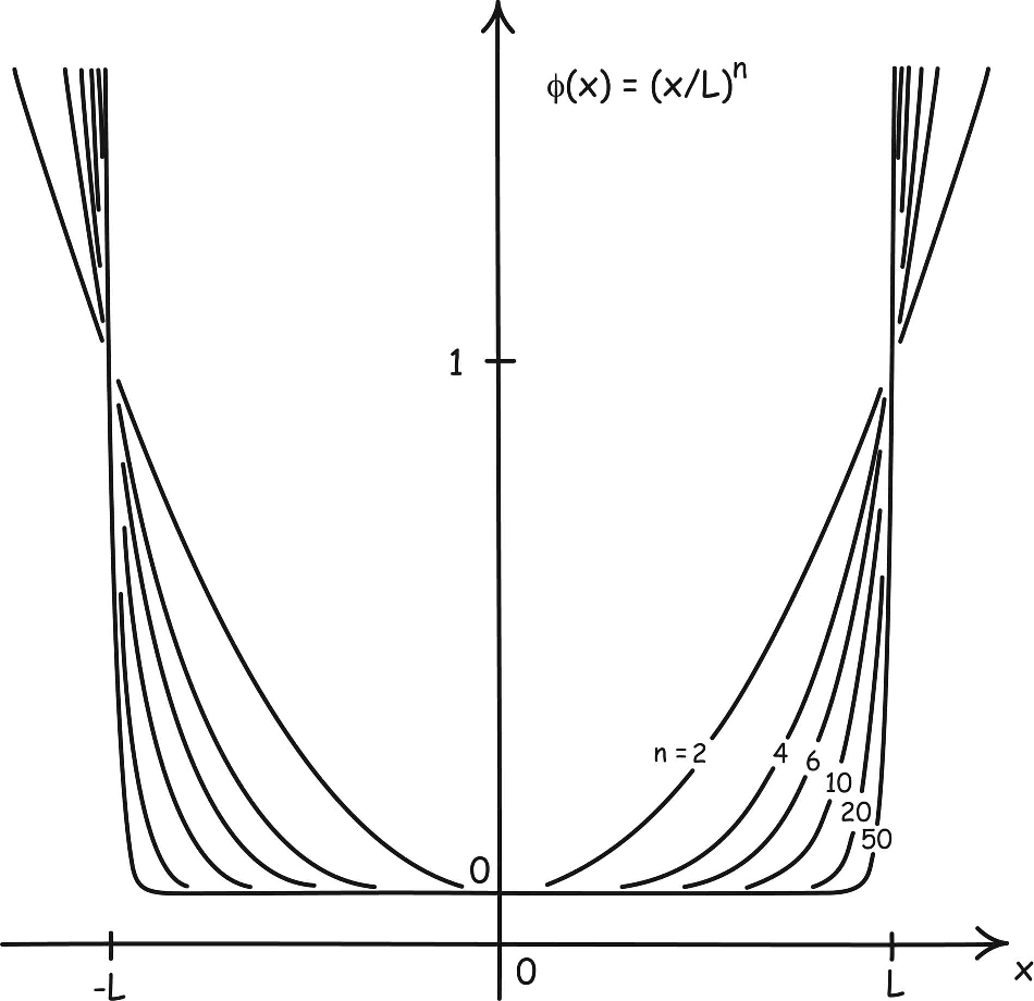
The mathematics of the partition functions is complicated even in simple cases. See Le Bellac et al. (Reference Le Bellac, Mortessagne and Batrouni2004, 183) and Jones (Reference Jones2006, sec. 3.1.3) for the simpler case of an Ising chain. The essential point, however, can be illustrated in a toy model. Imagine that, in some theory, a particle of type n generates a potential well of the form

where n = 1, 2, 3, … is always some finite, whole number. For each n, this potential well is an analytic function of the position coordinate x. When n grows large, however, will approach the limit of an infinitely high square well, as shown in figure 8:

Figure 8.

Analytic potential functions approach nonanalytic limit.

This limit function is not analytic (and not even continuous) but has been recovered from considerations of particles with finite n only. Moreover, the square well will approximate extremely well, especially when n is large, say 10²³.

Through an analogous infinite limit, we can recover nonanalytic functions from the functions governing arbitrarily large systems of finitely many components. These nonanalytic functions and their discontinuities have a pragmatic value only. If the atomic theory of matter is true, then ordinary thermal systems of finitely many components cannot display discontinuous changes in their thermodynamic properties. The changes they manifest are merely so rapid as to be observationally indistinguishable from discontinuous behavior.Footnote ¹³ Indeed, if we could establish that the phase transitions of real substances exhibit these discontinuities, we would have refuted the atomic theory of matter, which holds that ordinary thermal systems are composed of finitely many atoms, molecules, or components. It must be feared that a similar refutation is at hand, if the positing of infinitely many components is necessary to recover other observed behaviors of phase transitions.

5.2. Dispensable Idealizations

In section 4.3, it was argued that the renormalization group method analysis of phase transitions uses approximations only. Might we promote them to an idealization whose idealizing system has infinitely many components? What follows will show that there is no gain but a potential for harm.

This claims follows from the particular promotion procedure used to generate the idealization. In it, one takes a system and considers it to be a member of a set of like systems varying in some parameter. For phase transitions, the thermal system is taken to be one of many systems with arbitrarily many components. We consider a limit process governed by the parameter. For phase transitions, the number of components grows arbitrarily large. As the limit proceeds, we track the behavior of the systems’ properties and recover the limiting properties.

At this stage of the process, we already have a serviceable approximation of the target system in the form of these limit properties. These limit properties, it was argued in section 4.3, are all that is actually used in the renormalization group analysis of phase transitions. To complete the promotions, we now introduce an idealization of the original system in the form of the limit system. In the case of phase transitions, the limit system is one of infinitely many components.

Now the essential point: the limit system's properties must agree with the limit properties, else the promotion procedure fails. If these limits are well behaved, as in the case of the indefinitely elongated capsule of section 3.1, then the promotion succeeds. An infinite cylinder is a serviceable idealization of a very large capsule. The successful idealizations produced by this promotion procedure are dispensable. The resulting idealizations deliver nothing more than the inexact descriptions of the approximations provided by the limiting properties already determined in an earlier step of the procedure.

Mere dispensability is the best case. In many cases, however, this agreement of the limit system and limit properties fails. This failure would arise if we tried to use the continuum limit or the Boltzmann-Grad limit to generate an idealization. For in these cases, either there is no limit system or its properties differ markedly from the limit properties. We would have to dispense with the idealization and use the approximation provided by the limiting properties only.

In the case of phase transitions, at best, we do not know whether the limit system and limit properties agree. For, in general, we do not know whether the systems to which the infinite component Hamiltonians are attached carry the limit properties of those with finite component Hamiltonians. Investigating this agreement is not a standard part of a renormalization group analysis. We have some reason to expect the agreement to fail. In a few cases that have been worked out, such as those mentioned in section 4.1, it does fail. Extra conditions, peculiar to the infinite case, are needed to enforce specifically identified finite behaviors such as determinism. With this uncertainty, prudence indicates that we should dispense with the idealization, for the approximation already tells us what we could learn from the idealization about the target system. Persisting with the idealization merely risks the error of attributing properties to the limit system that it does not bear.

In short, the renormalization group analysis of phase transitions is a case in which all benefits are already accrued by the approximation. Promoting it to an idealization merely risks erroneous attributions for no gain.

5.3. Finite Systems Control Infinite Systems

The underlying moral is that the properties of finite systems control and that infinite systems cede to them when there is a conflict. One finds this view expressed in the physics literature. Lanford (Reference Lanford and Moser1975, 17) writes: “We emphasize that we are not considering the theory of infinite systems for its own sake so much as for the fact that this is the only precise way of removing inessential complications due to boundary effects, etc., i.e. we regard infinite systems as approximations to large finite systems rather than the reverse.” Fisher (Reference Fisher and Hahne1982, 14) portrays phase transitions with true discontinuities as unrealized in the laboratory and even experimentally refutable:

Le Bellac et al. (Reference Le Bellac, Mortessagne and Batrouni2004, 184) are similarly concerned to qualify their statement that the nonanalytic behavior of phase transitions occurs only in the thermodynamic limit: “The reader, who has undoubtedly observed an ice cube floating in a glass of water, may find this statement a bit surprising. What is meant by this statement is that the mathematical signature of a phase transition can only be seen in the infinite volume limit.”

The physics of phase transitions is complicated and difficult, and its philosophical analysis is rewarding. However, once one sees past the traps of the infinite limits, it is hard to find philosophical discontinuities.

In the venerable deductive-nomological (DN) or “covering law” account of explanation of Hempel and Oppenheim (Reference Hempel and Oppenheim1948), one explains some phenomenon by deducing it from physical laws with the assistance of particular conditions. The model has been widely and justly criticized, and there seems to be every reason to expect that the practice of explanation in science is so irregular as to admit no univocal account. However, there are a few cases in which the DN model works. The use of limits in statistical mechanics as approximations provides such a case. The phenomenon to be explained is, for example, universality: that many substances manifest the same critical exponents. Renormalization group methods take the theoretical framework of statistical mechanics as the covering law. They select as the particular conditions a broad class of Hamiltonians pertinent to the materials. They then derive universality under conditions close to criticality. The renormalization group analysis simply is a covering law explanation.

While the ontological reduction of ordinary matter to atoms, molecules, and the like is as secure as any result of science, we cannot have the same confidence for explanatory reduction. The traffic in Los Angeles may ontologically be nothing but atoms, molecules, and heat radiation. Yet we cannot expect their statistical mechanics to provide an explanation of traffic jams. Nagel's (Reference Nagel1961, chap. 11) is the venerable account of reduction in which the less fundamental theory is derived from the more fundamental. It too has been much criticized and justly so. However, there are a few cases in which it still seems to apply.Footnote ¹⁴ In providing a covering law explanation of critical exponents, renormalization group methods are also providing a Nagel-style reduction, or at least something like it, such as the more sophisticated version of Schaffner (Reference Schaffner1967).

Finally, the idea that discontinuous changes of phase transitions are emergent phenomena is difficult to penetrate, for the phenomena at issue are not possible objects of experience. Real phase transitions cannot exhibit the discontinuities on pain of contradicting the atomic theory of matter, and, were the discontinuities established factually, the atomic theory would fall.